Global nutrient transport in a world of giantsChristopher E. Doughtya,1, Joe Romanb,c, Søren Faurbyd, Adam Wolfe, Alifa Haquea, Elisabeth S. Bakkerf,Yadvinder Malhia, John B. Dunning Jr.g, and Jens-Christian Svenningd

aEnvironmental Change Institute, School of Geography and the Environment, University of Oxford, Oxford OX1 3QY, United Kingdom; bOrganismic andEvolutionary Biology, Harvard University, Cambridge, MA 02138; cGund Institute for Ecological Economics, University of Vermont, Burlington, VT 05445;dSection of Ecoinformatics & Biodiversity, Department of Bioscience, Aarhus University, DK-8000 Aarhus C, Denmark; eDepartment of Ecology andEvolutionary Biology, Princeton University, Princeton, NJ 08544; fDepartment of Aquatic Ecology, Netherlands Institute of Ecology, 6708 PB Wageningen,The Netherlands; and gDepartment of Forestry and Natural Resources, Purdue University, West Lafayette, IN 47907

Edited by John W. Terborgh, Duke University, Durham, NC, and approved August 6, 2015 (received for review March 14, 2015)

The past was a world of giants, with abundant whales in the sea andlarge animals roaming the land. However, that world came to an endfollowingmassive late-Quaternary megafauna extinctions on land andwidespread population reductions in greatwhale populations over thepast few centuries. These losses are likely to have had important con-sequences for broad-scale nutrient cycling, because recent literaturesuggests that large animals disproportionately drive nutrient move-ment. We estimate that the capacity of animals to move nutrientsaway from concentration patches has decreased to about 8% of thepreextinction value on land and about 5% of historic values in oceans.For phosphorus (P), a key nutrient, upward movement in the ocean bymarinemammals is about 23%of its former capacity (previously about340 million kg of P per year). Movements by seabirds and anadromousfish provide important transfer of nutrients from the sea to land,totalling ∼150 million kg of P per year globally in the past, a transferthat has declined to less than 4% of this value as a result of thedecimation of seabird colonies and anadromous fish populations.We propose that in the past, marine mammals, seabirds, anadromousfish, and terrestrial animals likely formed an interlinked systemrecycling nutrients from the ocean depths to the continental in-teriors, with marine mammals moving nutrients from the deepsea to surface waters, seabirds and anadromous fish moving nu-trients from the ocean to land, and large animals moving nutri-ents away from hotspots into the continental interior.

biogeochemical cycling | extinctions | megafauna | whales |anadromous fish

There were giants in the world in those days.

Genesis 6:4, King James version

The past was a world of giants, with abundant whales in theoceans and terrestrial ecosystems teeming with large animals.

However, most ecosystems lost their large animals, with around150 mammal megafaunal (here, defined as ≥44 kg of body mass)species going extinct in the late Pleistocene and early Holocene(1, 2). These extinctions and range declines continued up throughhistorical times and, in many cases, into the present (3). No globalextinctions are known for any marine whales, but whale densitiesmight have declined between 66% and 99% (4–6). Some of thelargest species have experienced severe declines; for example, inthe Southern Hemisphere, blue whales (Balaenoptera musculus)have been reduced to 1% of their historical numbers as a result ofcommercial whaling (4). Much effort has been devoted to de-termining the cause of the extinctions and declines, with less effortfocusing on the ecological impacts of the extinctions. Here, wefocus on the ecological impacts, with a specific focus on hownutrient dynamics may have changed on land following the late-Quaternary megafauna extinctions, and in the sea and air followinghistorical hunting pressures.Most biogeochemists studying nutrient cycling focus on in situ

production, such as weathering or biological nitrogen (N) fixation,largely ignoring lateral fluxes by animals because they are consid-ered of secondary importance (3). The traditional understanding ofbiogeochemistry is that “rock-derived” nutrients originate with the

weathering of primary rock. These nutrients are then lost to thehydrosphere by leaching or runoff or to the atmosphere by dust,fire, or volatilization. These nutrients slowly make their way to theoceans, where they are buried at the bottom of the sea. Eventually,these sediments are subducted, transformed to metamorphic origneous rock, and uplifted to be weathered once again. We are leftwith an impression that nutrient cycling in adjacent landscapes orgyres is disconnected except through the atmosphere or hydro-sphere, and that animals play only a passive role as consumers ofnutrients. However, this notion may be a peculiar world view thatcomes from living in an age where the number and size of animalshave been drastically reduced from their former bounty. We mustwonder: What role do animals play in transporting nutrients lat-erally across ecosystems on land, vertically through the ocean, oracross the ocean land divide?Animal digestion accelerates cycling of nutrients from more

recalcitrant forms in decomposing plant matter to more labileforms in excreta after (wild or domestic) herbivore consumption onland (7). For instance, nutrients can be locked in slowly decom-posing plant matter until they are liberated for use through animalconsumption, digestion, and defecation. This process has beentheorized to have played a large role in the Pleistocene steppes ofSiberia. Abundant large herbivores ate plants that were rapidlydecomposed in their warm guts, liberating the nutrients to be reused.However, following extinctions of these animals, nutrients were hy-pothesized to have been locked into plant matter that is decomposingonly slowly, making the entire ecosystem more nutrient-poor (8).Similarly, at present times, large herbivores enhance nutrient cyclingin the grazing lawns of the Serengeti (9).What role do animals play in the spatial movement of nutrients?

This question is especially pertinent because animals are most likelyto influence the flow of nutrients that are in short supply. There arenow a large number of site-level studies that have demonstrated how

Significance

Animals play an important role in the transport of nutrients,but this role has diminished because many of the largest ani-mals have gone extinct or experienced massive populationdeclines. Here, we quantify the movement of nutrients by an-imals in the land, sea, rivers, and air both now and prior to theirwidespread reductions. The capacity to move nutrients awayfrom hotspots decreased to 6% of past values across land andocean. The vertical movement of phosphorus (P) by marinemammals was reduced by 77% and movement of P from sea toland by seabirds and anadromous fish was reduced by 96%,effectively disrupting an efficient nutrient distribution pumpthat once existed from the deep sea to the continental interiors.

Author contributions: C.E.D. designed research; C.E.D. performed research; J.R., S.F., A.W.,J.B.D., and J.-C.S. contributed new reagents/analytic tools; C.E.D., A.W., and A.H. analyzeddata; and C.E.D., J.R., E.S.B., Y.M., J.B.D., and J.-C.S. wrote the paper.

The authors declare no conflict of interest.

This article is a PNAS Direct Submission.1To whom correspondence should be addressed. Email: chris.doughty@ouce.ox.ac.uk.

This article contains supporting information online at www.pnas.org/lookup/suppl/doi:10.1073/pnas.1502549112/-/DCSupplemental.

www.pnas.org/cgi/doi/10.1073/pnas.1502549112 PNAS Early Edition | 1 of 6

ECOLO

GY

SPEC

IALFEATU

RE

animals move nutrients from one site to another or across ecosystemboundaries. For example, moose (Alces americanus) transfer signif-icant amounts of aquatic-derived N to terrestrial systems, whichlikely increases terrestrial N availability in riparian zones (10). Ter-restrial predators (e.g., bears, otters, and eagles) feeding on anad-romous fish that move from the ocean to freshwater to spawn cantransport ocean-derived nutrients to terrestrial ecosystems, a processthat has been verified by isotopic analysis (11). Hippopotamuses(Hippopotamus amphibius) supplement aquatic systems with terres-trial-derived nutrients, which strongly enhance aquatic productivity(12). Seabirds transport nutrients from the sea to their breedingcolonies onshore (13, 14). Studies have documented increases of soilphosphorus (P) concentrations on seabird islands compared withnon-seabird islands that were much stronger than for soil %N andpresent in soils for up to thousands of years (14). In some sites, in-creased soil P more than doubled plant P concentrations, but thisconcentration varied substantially from site to site (14). Further-more, seabirds and marine mammals play an important role as nu-trient vectors aiding in the redistribution of micronutrients, such asiron (Fe) (15). Despite their vastly decreased numbers, the impor-tant role of whales in distributing nutrients is just now coming tolight. Whales transport nutrients laterally, in moving between feedingand breeding areas, and vertically, by transporting nutrients fromnutrient-rich deep waters to surface waters via fecal plumes andurine (16–18). Studies in the Gulf of Maine show that cetaceans andother marine mammals deliver large amounts of N to the photiczone by feeding at or below the thermocline and then excreting ureaand metabolic fecal N near the surface (17).More recently, studies have demonstrated that animals can dif-

fuse significant quantities of nutrients from areas of high nutrientconcentration to areas of lower nutrient concentration even with-out mass flow of feces out of the fertile area. For instance, woollymonkeys (Lagothrix lagotricha) in Amazonia transported more Pthan arrives from dust inputs across a floodplain concentrationgradient, without preferentially defecating in the less fertile area,merely by eating and defecating back and forth across the nutrientconcentration gradient (19). If a small single species can transportsuch significant quantities of P, what is the role of all animals in anecosystem over long periods of time? Two recent studies compiledsize relationship data for terrestrial mammals within a random-walk mathematical framework and found that the distribution ofnutrients away from a concentration gradient is size-dependent,with larger animals having disproportionally greater importance tothis flow of nutrients than smaller animals (20, 21). For the Am-azon basin, it was estimated that the extinction of the megafaunamay have led to a >98% reduction in the lateral transfer flux of thelimiting nutrient P, with large impacts on ecosystem P concentra-tions in regions outside of the fertile floodplains (20, 21).If large animals are of disproportionate importance, then the

obvious question is: What was this nutrient movement like in thepast, in a world of giants, when mean animal size was much greateron land and at sea? Furthermore, what was the role of animals inreturning nutrients from sea to land, against the passive diffusiongradients? Seabirds and anadromous fish are two important animalgroups for the transport of nutrients from sea to land. Both groupsare also facing pressure, and 27% of all seabirds are classified asthreatened (critically endangered, endangered, or vulnerable), andthe largest of all seabirds, the albatross, is the most endangered,with up to 75% of albatross species considered threatened or en-dangered (22–24)]. Likewise, populations of anadromous fish havedeclined to less than 10% of their historical numbers in the PacificNorthwest (25) and both the northeastern and northwestern Atlantic(26, 27). There have been many individual site-level studies showingthe importance of animals in distributing nutrients, but as far as weare aware, no previous study has attempted to estimate at a globalscale how this distribution has changed from the time before human-caused extinctions and exploitation up to today in the oceans, air,rivers, and land. In this study, we aim to estimate three things: (i) thelateral nutrient distribution capacity of terrestrial and marinemegafauna, (ii) the global vertical flux of nutrients to surface watersby marine megafauna, and (iii) the global flux of nutrients by sea-birds and anadromous fish from the sea to land.

ResultsLateral Nutrient Distribution Capacity by Terrestrial Mammals andWhales. We used a “random walk” mathematical formulation (28)(mathematically formulated in Eq. 1 inMethods and SI Appendix) tocalculate a global per pixel nutrient diffusivity in units of square ki-lometers per year (these units are of diffusivity and signify the abilityof nutrients to move away from a nutrient concentration gradient,just like thermal diffusivity indicates the ability of a surface to moveheat away from a hot area). We estimate that the global mean nu-trient distribution capacity before the late-Quaternary extinctionsaveraged 180,000 km2·y−1 on the land surface and that it is currently16,000 km2·y−1, ∼8% of its former value (Table 1; detailed meth-odology is provided in Methods and SI Appendix). However, there ismuch regional variation. For example, in parts of Africa, such asKruger National Park in South Africa, capacity is still close to 100%of what it once was in the Late Pleistocene, whereas other regions,such as southern South America, are at less than 0.01% of previousvalues (Fig. 1). Before the extinctions, nutrient distribution capacitywas much more evenly spread than it is currently, with most ofthe current capacity only in Africa, where extensive megafaunaremain. Every continent outside Africa (Africa is at 46% of its late-Quaternary value) is at less than 5% of the original value, with thelargest change in South America (∼1% of the original value; Table1). Historical range reduction of species also played an importantrole in the decrease of the lateral nutrient flux, and we estimatethat without the range reduction of large species (excluding allextinctions) the capacity would be 37% higher compared with to-day’s baseline. Each estimated value is based on a number of as-sumptions that we explore in a sensitivity study (SI Appendix,Tables 1 and 2).

Nutrient Movement by Marine Mammals. We calculated lateral dif-fusion capacity for 13 species of great whales (SI Appendix, Table 3)and estimated that the capacity in the Southern Ocean is 2% of itshistorical value, with slightly higher values in the North Pacific(10%) and the North Atlantic (14%) (Fig. 2 A–C and Table 1).Mean nutrient diffusion capacity is larger for the great whalesthan for terrestrial animals at natural capacity (640,000 km2·y−1for great whales vs. 180,000 km2·y−1 for terrestrial mammals).Because of their enormous size and high mobility (and despitehaving many fewer species), great whales might have once trans-ported nutrients away from concentration gradients more efficientlythan terrestrial mammals.Marine mammals can also distribute nutrients vertically in oceans

(Fig. 2 D–F). We calculate nutrient fluxes caused by animals interms of the frequently limiting nutrient, P, which serves as a proxyfor other limiting elements, such as N and Fe. We calculate thisvertical distribution of nutrients for nine marine mammals (SIAppendix, Table 4) and find that they moved a global total of∼340 million (260–430 million; SI Appendix, Table 2) kg of P peryear from the depth to the surface waters before widespread huntingand that they now move ∼75 million (54–110 million; SI Appendix,Table 2) kg of P per year, representing a decrease to 23% of originalcapacity (Fig. 2 D–F and Table 1). We also found vast regionaldifferences: Vertical transport capacity in the Southern Ocean is now∼16% of its historical value, but there are higher values in the NorthPacific (34%) and the North Atlantic (28%). We compare our es-timates of P movement at natural capacity by marine mammals withquantities of ocean P concentrations that were measured by theOcean Climate Laboratory (details are provided in SI Appendix) andestimate that on a yearly basis, in the past, marine mammals couldhave increased surface concentrations by up to 1% per year in theSouthern Ocean [2.5 kg·km−2·y−1 added to a mean concentra-tion of 248 kg·km−2, although other calculations have suggestedthat the effect on trace elements could be even higher (29)], whichcould result in considerable stock changes in surface P over time.

Nutrient Distribution from the Ocean to Land by Seabirds and Anad-romous Fish. Based on global range maps of seabirds and theirbody masses, we calculate coastal consumption by seabirdsand assume 20% (5 to 35%) of guano reaches land (methods on

2 of 6 | www.pnas.org/cgi/doi/10.1073/pnas.1502549112 Doughty et al.

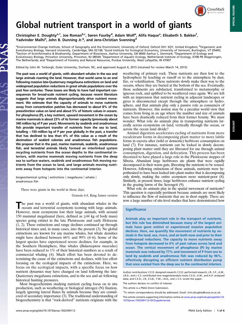
how 20% was calculated are provided in SI Appendix). Thereforeglobal averaged sea-to-land movement of P is 0.19 ± 0.15 kg ofP km−2·y−1 in coastal regions, but varies by an order of magnitudethroughout the planet, with peaks in the Southern Hemisphere(Fig. 3 and Table 1). These estimates are calculated based ontheoretical population densities (30), and it is probably closer totheoretical historical values than to actual values today. Whenaveraged by coastal continental area, we find a maximum inOceania, with 0.31 ± 0.23 kg of P km−2·y−1, and lower values inNorth America, with 0.16 ± 0.12 kg of P km2·y−1. We calculate aglobal flux of 6.3 million (1.5–16 million; SI Appendix, Table 2)kg km−2·y−1 of P from sea to land by the seabirds, with almosthalf moving onto the Eurasian landmass (Table 1).It is estimated that there are 110 species of anadromous fish,

such as salmon, that migrate from oceans to rivers to breed andeventually die (SI Appendix, Table 5) (31). Using range maps for42 of these species, and an additional 47 closely related speciesas proxies for the missing range maps, we estimate that, histor-ically, anadromous fish may have moved at least an order ofmagnitude more P from ocean to land [140 million (71–430million) km2·y−1; SI Appendix, Table 2] than seabirds [6.3 mil-lion (1.5–16 million) km2·y−1; SI Appendix, Table 2], but this esti-mated value has decreased to ∼4% (5.6 million km2·y−1) of theoriginal value. These values are not evenly distributed, and thereare much higher values in the Northern Hemisphere and at highlatitudes than in more tropical latitudes. Each value has manyuncertainties involved in its calculation, which we explore in asensitivity study (SI Appendix, Tables 1 and 2).

DiscussionWe estimate that the decimation of terrestrial megafauna andwhales has reduced the ability of animals to distribute nutrientsaway from regions of nutrient abundance to ∼6% of global naturalcapacity. Did this change make the planet less fertile? We do notcalculate changes to fertility from lateral diffusivity declines be-cause accurate global maps of nutrient hotspots necessary for sucha calculation do not exist at the necessary resolution. Previousexperimental studies, however, have found that animals movesignificant quantities of nutrients across concentration gradientsdespite not necessarily moving dung from fertile to nonfertileareas (11, 14, 19). Regional models found that the transfer of Paway from the Amazonian floodplains may have dropped by morethan 50% following the extinction of the Amazonian megafauna(20, 21). We hypothesize that such a drop in nutrient diffusioncapacity would have decreased nutrient concentrations in regionsthat are distant from their abiotic sources (deposited by eitherwind or water), resulting in broad global regions being less fertile.On land, large disparities in animal sizes and total animal

numbers led to differences in nutrient distribution capacity bothbefore and following the extinctions due to regional disparities inextinctions. For instance, South America once had the largestnutrient distribution capacity, but following the Late-Pleistoceneextinctions, it experienced the largest drop, to ∼1% of its originalcontinent-wide capacity. With accurate megafauna range maps,we can pinpoint regions with especially large drops. For instance,southern South America once had the largest number ofmegaherbivores (>1,000 kg, n = 15), all of which went extinct (32).This large number of megaherbivores gave it, before the extinctions,the largest estimated present natural lateral diffusion capacity of

Table 1. Average global and regional estimates of nutrient distribution capacity (km2·y−1) for terrestrial mammals and whales, andglobal and regional estimates of vertical nutrient movement of P (kg·y−1) by all diving marine mammals and sea-to-land totalP movement (kg·y−1) by seabirds and anadromous fish

UnitsTotal landaverage

Totaloceanaverage Africa Australia Eurasia

NorthAmerica

SouthAmerica

SouthernOcean

NorthAtlantic

NorthPacific

Nutrient distribution capacity

Pastmean,km2·y−1

Landmammals1.8e5

Greatwhales6.4e5

Landmammals1.28e5

Landmammals0.15e5

Landmammals2.77e5

Landmammals2.39e5

Landmammals1.53e5

Greatwhales11e5

Greatwhales4.0e5

Greatwhales2.7e5

Currentmean,km2·y−1

1.6e4 3.2e4 6.67e4 467 1.13e4 0.42e4 0.17e4 0.22e5 0.57e5 0.25e5

% 8% 5% 46% 3% 4% 2% 1% 2% 14% 10%

P movement

Past total,kg P·y−1

A. fish1.4e8kg·y−1

Marinemammals3.4e8kg·y−1

A. fish1.9e6kg·y−1

A. fish0.4e6kg·y−1

A. fish69e6kg·y−1

A. fish51e6kg·y−1

A. fish0.5e6kg·y−1

Marinemammals1.7e8

Marinemammals0.9e8

Marinemammals0.7e8

Seabirds6.3e6 ±5e6

Seabirds0.89e6 ±0.66e6

Seabirds0.79e6 ±0.6e6

Seabirds2.4e6 ±1.8e6

Seabirds0.99e6 ±0.7e6

Seabirds0.89e6 ±0.6e6

Currenttotal,kg P·y−1

A. fish5.6e6

Marinemammals7.9e7kg·y−1

A. fish0.1e6

A. fish0.01e6

A. fish3.2e6

A. fish2.3e6

A. fish0.02e6

2.8e7 2.6e7 2.4e7

% 4% 23% NA NA NA NA NA 16% 28% 34%

(Top) Average global and regional estimates of nutrient distribution capacity (km2·y−1) based on Eq. 1 for terrestrial mammals and for whales (SI Appendix,Table 3). Percentages are the current value divided by the past value. (Bottom) Global and regional estimates of vertical nutrient movement of P (kg·y−1) by alldiving marine mammals (SI Appendix, Table 4) and sea-to-land total P movement (kg·y−1) by seabirds and anadromous (A.) fish (SI Appendix, Table 5). Weassume that 20% (ranging between 5% and 35%) of seabird guano produced arrives on coastal land. We assume our calculations for seabird populations arerepresentative of past, not current, populations because they are based on theoretical population densities (43). NA (not available) represents regions wherethere are not sufficient data for an estimate. A sensitivity study for each number is provided in SI Appendix, Tables 1 and 2.

Doughty et al. PNAS Early Edition | 3 of 6

ECOLO

GY

SPEC

IALFEATU

RE

anywhere in the world. However, currently, with the largest animalsin South America only weighing up to ∼300 kg, continental nutrientdistribution capacity has dropped to ∼0.01% of its original value insome regions. However, in some regions, exotic and mainly do-mesticated ungulates may have partially taken over this role (33).Therefore, because southern South America had the largest changein capacity by animals to move nutrients away from abiotic sources,it may be a good test region to look for such changes in long-termnutrient deposition.Marine mammals have seen broad population reductions due to

widespread hunting over the past few hundred years (34). Such pop-ulation decreases reduced the lateral distribution capacity and perhapsreduced the vertical distribution, allowing more nutrients to dropbelow the photic zone. This ability to spread nutrients vertically maybe especially important, because once nutrients drop below the photiczone and into the deep ocean sediments, they are generally consideredto be lost to the surface biota, and only tectonic movements andlimited regions where water is uplifted, will further recycle them(16). Aquatic algae, which conduct most of the ocean’s photosyn-thesis, have a much faster turnover time than land plants due to

their often single-cellular nature, and due to this faster turnovertime, nutrients, especially limiting nutrients, should be converted toprimary producer biomass more quickly in the oceans. Further-more, a much larger share of primary production in oceans (algae)is consumed compared with terrestrial primary producers (35). Thenutrients transported by whales, or as a consequence of whale ac-tivity, should be assimilated more rapidly, and contribute to systemproductivity more directly than on land. Also, whales and their preymay help in retaining limiting nutrients (N, P, and Fe) in the surfacelayer and releasing these nutrients slowly into the water (18).Seabirds may act as a link connecting nutrient concentrations in

the oceans with nutrient concentrations on the land. Here, we haveestimated that seabirds can increase P concentrations in coastalenvironments globally by ∼6 million kg·y−1 through the depositionof guano. Guano is generally deposited on steep cliffs or offshoreislands generally inaccessible to most terrestrial animals. However,over long time scales, these nutrients may become accessible toterrestrial fauna as sea levels drop during the ice ages and sea cliffserode. This flux of nutrients has almost certainly decreased throughtime as seabird populations have decreased [27% of seabirds areclassified as threatened (22)] or gone extinct (e.g., the great auk,Pinguinus impennis) often due to, for instance, invasive mammalpredators decimating seabird colonies (36). In the past, scavengingbirds, such as condors, may also have acted as vectors of nutrientsfrom the sea to the land. For example, during the Pleistocene,isotope data suggest that California condors (Gymnogyps cal-ifornianus) fed on both terrestrial megafauna and marine mam-mals, but by the late 1700s, condor diets had shifted predominantlyto terrestrial animals because there were fewer marine mammals tobe harvested after likely having subsisted on marine carcasses acrossthe Holocene, with inland populations going extinct at the end ofthe Pleistocene (37). This flux has certainly greatly decreased asboth marine mammals and large scavengers have seen their num-bers drop substantially (38).Possibly, a more important form of sea-to-land nutrient trans-

port comes from the migratory behavior of anadromous fish, whichwe estimate to bring at least an order of magnitude more nutrientsfrom oceans to land than do seabirds. However, they have alsoexperienced drastic population losses (25–27), and we estimate thatthe current nutrient flux is less than 4% of historic values, beforeoverfishing and habitat modification, such as damming of rivers.Anadromous fish seem to be especially important vectors of nutrients

100%10%1%0.1%0.01%

Percent of original

Current Log10 Phi (km2 yr-1)

Log10 Phi (km2 yr-1)

Past

Fig. 1. Lateral nutrient distribution capacity (km2·y−1) by terrestrial mam-mals. Lateral diffusion capacity (Φ; Eq. 1) of nutrients by all mammals as itwould have been without the end-Pleistocene and Holocene megafaunaextinctions and extirpations (Top), as it is currently (Middle), and as the per-centage of the original value (Bottom).

Log1

0 Ph

i (km

2yr

-1)

current

past

Percent of original Percent of original

past

currentLo

g10

Kg P

km-2

yr-1

Log1

0 Kg

Pkm

-2 yr

-1

Great whale pump Deep-diving mammalsA

B

C

D

E

F

Log1

0 Ph

i (km

2yr

-1)

% o

f orig

inal

% o

f orig

inal

Fig. 2. Horizontal and vertical nutrient distribution capacity by greatwhales. Lateral movement capacity (Φ, km2·y−1; Eq. 1) by great whales (listedin SI Appendix, Table 3) for past whale densities before widespread humanhunting (A), current whale densities (B), and the percentage of the originalvalue (i.e., current values divided by past values) (C). Vertical movement ofnutrients by marine mammals (listed in SI Appendix, Table 4), log10 kilo-grams of P per square kilometer per year (kg·Pkm−2·y−1), for past marinemammal densities before widespread human hunting (D), current marinemammal densities (E), and the percentage of the original value (F).

4 of 6 | www.pnas.org/cgi/doi/10.1073/pnas.1502549112 Doughty et al.

because they travel much further inland than seabirds (Fig. 3). It isuncertain what quantity of nutrients transported inland by the fisharrives onto terra firma, but it is clearly a function of river size,distance transported inland, and consumption of the fish by scaven-gers and predators. However, isotopic evidence indicates thatsignificant quantities of ocean-derived nutrients from anad-romous fish do enter terrestrial ecosystems (11). This loss of nu-trients to these ecosystems from historic highs may have affectedthe entire ecosystem, including the fish themselves, and “con-tributed to the downward spiral of salmonid abundance and di-versity in general” (25). We estimate the total flux of P from sea toland by anadromous fish and seabirds in the past (146 million kg ofP per year) is still much less than the total P consumed by humansfor fertilizers each year [48,500 million kg of phosphoric acid (asP2O5) in 2010 and growing at 1.9% per year (39)].Before the widespread extinction of megafauna and hunting of

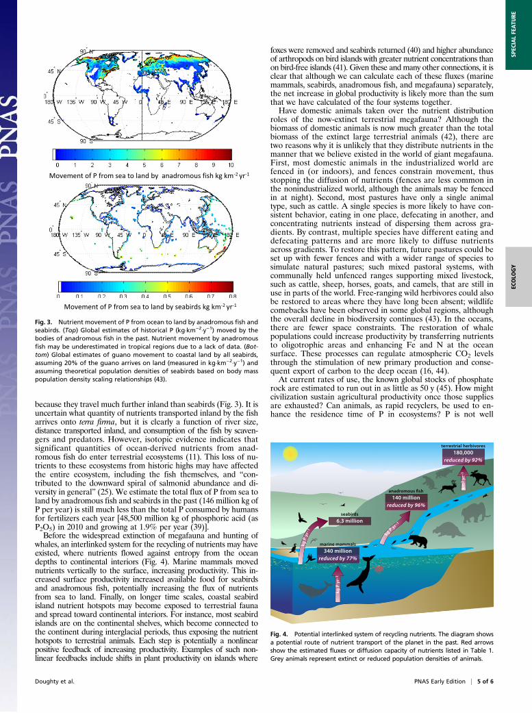
whales, an interlinked system for the recycling of nutrients may haveexisted, where nutrients flowed against entropy from the oceandepths to continental interiors (Fig. 4). Marine mammals movednutrients vertically to the surface, increasing productivity. This in-creased surface productivity increased available food for seabirdsand anadromous fish, potentially increasing the flux of nutrientsfrom sea to land. Finally, on longer time scales, coastal seabirdisland nutrient hotspots may become exposed to terrestrial faunaand spread toward continental interiors. For instance, most seabirdislands are on the continental shelves, which become connected tothe continent during interglacial periods, thus exposing the nutrienthotspots to terrestrial animals. Each step is potentially a nonlinearpositive feedback of increasing productivity. Examples of such non-linear feedbacks include shifts in plant productivity on islands where

foxes were removed and seabirds returned (40) and higher abundanceof arthropods on bird islands with greater nutrient concentrations thanon bird-free islands (41). Given these andmany other connections, it isclear that although we can calculate each of these fluxes (marinemammals, seabirds, anadromous fish, and megafauna) separately,the net increase in global productivity is likely more than the sumthat we have calculated of the four systems together.Have domestic animals taken over the nutrient distribution

roles of the now-extinct terrestrial megafauna? Although thebiomass of domestic animals is now much greater than the totalbiomass of the extinct large terrestrial animals (42), there aretwo reasons why it is unlikely that they distribute nutrients in themanner that we believe existed in the world of giant megafauna.First, most domestic animals in the industrialized world arefenced in (or indoors), and fences constrain movement, thusstopping the diffusion of nutrients (fences are less common inthe nonindustrialized world, although the animals may be fencedin at night). Second, most pastures have only a single animaltype, such as cattle. A single species is more likely to have con-sistent behavior, eating in one place, defecating in another, andconcentrating nutrients instead of dispersing them across gra-dients. By contrast, multiple species have different eating anddefecating patterns and are more likely to diffuse nutrientsacross gradients. To restore this pattern, future pastures could beset up with fewer fences and with a wider range of species tosimulate natural pastures; such mixed pastoral systems, withcommunally held unfenced ranges supporting mixed livestock,such as cattle, sheep, horses, goats, and camels, that are still inuse in parts of the world. Free-ranging wild herbivores could alsobe restored to areas where they have long been absent; wildlifecomebacks have been observed in some global regions, althoughthe overall decline in biodiversity continues (43). In the oceans,there are fewer space constraints. The restoration of whalepopulations could increase productivity by transferring nutrientsto oligotrophic areas and enhancing Fe and N at the oceansurface. These processes can regulate atmospheric CO2 levelsthrough the stimulation of new primary production and conse-quent export of carbon to the deep ocean (16, 44).At current rates of use, the known global stocks of phosphate

rock are estimated to run out in as little as 50 y (45). How mightcivilization sustain agricultural productivity once those suppliesare exhausted? Can animals, as rapid recyclers, be used to en-hance the residence time of P in ecosystems? P is not well

Movement of P from sea to land by seabirds kg km-2 yr-1

Movement of P from sea to land by anadromous fish kg km-2 yr-1

Fig. 3. Nutrient movement of P from ocean to land by anadromous fish andseabirds. (Top) Global estimates of historical P (kg·km−2·y−1) moved by thebodies of anadromous fish in the past. Nutrient movement by anadromousfish may be underestimated in tropical regions due to a lack of data. (Bot-tom) Global estimates of guano movement to coastal land by all seabirds,assuming 20% of the guano arrives on land (measured in kg·km−2·y−1) andassuming theoretical population densities of seabirds based on body masspopulation density scaling relationships (43).

kgP

yr–1

kg P

yr–

1

6.3 million

340 millionreduced by 77%

140 millionreduced by 96%

180,000reduced by 92%

seabirds

marine mammals

terrestrial herbivores

kg

P yr–1

km2

yr–1

Fig. 4. Potential interlinked system of recycling nutrients. The diagram showsa potential route of nutrient transport of the planet in the past. Red arrowsshow the estimated fluxes or diffusion capacity of nutrients listed in Table 1.Grey animals represent extinct or reduced population densities of animals.

Doughty et al. PNAS Early Edition | 5 of 6

ECOLO

GY

SPEC

IALFEATU

RE

distributed, and it causes eutrophication in some areas, whereasP deficits still affect almost 30% of the global cropland area(46, 47). Therefore, a redistribution of P from areas where it iscurrently found in excess to areas where the soil is naturallyP-poor may simultaneously boost global crop production and reduceeutrophication (47). Animals play a key role in nutrient movementon the land and in the sea, rivers, and air. Although the numberswe have calculated in this paper are exploratory (we explore thisuncertainty in SI Appendix, Tables 1 and 2) and subject to furtherresearch and quantification, we have demonstrated the plausibilityof an animal-mediated chain of nutrient transfer that connects thedeep ocean to the continental interiors. We have shown that aworld teeming with large animals may have had an efficient systemof redistributing P. Some restoration of this important processcould be aided with fenceless pastures with greater livestock bio-diversity, restoration of great whales to their historic numbers, andrestoration of seabird colonies and anadromous fish populations.

MethodsLateral nutrient distribution capacity was mathematically formulated and foundto be strongly size-dependent in two previous papers (20, 21), and this mathe-matical framework is reformulated in SI Appendix. We now use this framework tocalculate how the ability of land mammals and great whales to diffuse nutrientsaway from hotspots may have changed following the widespread extinctions of

megafauna and hunting of whales. We estimate the total capability of animals todistribute nutrients both now, with the current International Union for Conser-vation of Nature (IUCN) species range maps and body mass, and in the past forthe now-extinct Pleistocene megafauna, using a dataset of the ranges and bodymasses of extinct megafauna (48, 49).We use the following equation to estimatediffusion capacity (completely described in SI Appendix) based on mass (M) andthe scaling parameters of day range (DD), metabolic rate (MR), populationdensity (PD), and food passage time (PR) (this equation differs slightly from ourprevious formulation by excluding parameters not dependent on animal mass):

Φ=MR*PD*ðDD* PRÞ2

2*PR= 0.78*0.05*M1.17. [1]

Weestimate verticalmovement of nutrients bymarinemammals and sea-to-landnutrient fluxby seabirds andanadromous fish basedon IUCN species rangemaps,mean body size, and scaling relationships for metabolic consumption andpopulation densities (detailed methodology is provided in SI Appendix).

ACKNOWLEDGMENTS. A. Zerbini provided helpful comments on whale pop-ulations. J.-C.S. was supported by Grant ERC-2012-StG-310886-HISTFUNC from theEuropean Research Council (ERC). Additionally, we consider this article to be acontribution to the Danish National Research Foundation Niels Bohr ProfessorshipProject, Aarhus University Research on the Anthropocene. Y.M. was supported byan ERC Advanced Investigator Award and by the Jackson Foundation. J.R. wassupported by a Sarah and Daniel Hrdy Visiting Fellowship in Conservation Biologyat Harvard University. C.E.D. acknowledges funding from the John Fell Fund.

1. Sandom C, Faurby S, Sandel B, Svenning JC (2014) Global late Quaternary megafaunaextinctions linked to humans, not climate change. Proc Biol Sci 281(1787):20133254.

2. Barnosky AD, Koch PL, Feranec RS, Wing SL, Shabel AB (2004) Assessing the causes of

late Pleistocene extinctions on the continents. Science 306(5693):70–75.3. Dirzo R, et al. (2014) Defaunation in the Anthropocene. Science 345(6195):401–406.4. Christensen LB (2006) Marine mammal populations: Reconstructing historical abun-

dances at the global scale. Fisheries Centre Research Reports 14(9):1–161.5. Branch TA, Williams TM (2007) Legacy of industrial whaling: Could killer whales be re-

sponsible for declines of sea lions, elephant seals, and Minke whales in the SouthernHemisphere? Whales, Whaling, and Ocean Ecosystems, eds Estes JA, DeMaster DP,

Doak DF, Williams TM, Brownell RL (Univ of California Press, Oakland, CA), pp 262–278.6. McCauley DJ, et al. (2015) Marine defaunation: Animal loss in the global ocean.

Science 347(6219):1255641.7. Hobbs NT (1996) Modification of ecosystems by ungulates. J Wildl Manage 60(4):695–713.8. Zimov SA, et al. (1995) Steppe-tundra transition—A herbivore-driven biome shift at

the end of the Pleistocene. Am Nat 146(5):765–794.9. McNaughton SJ, Banyikwa FF, McNaughton MM (1997) Promotion of the cycling of

diet-enhancing nutrients by African grazers. Science 278(5344):1798–1800.10. Bump JK, Tischler KB, Schrank AJ, Peterson RO, Vucetich JA (2009) Large herbivores

and aquatic-terrestrial links in southern boreal forests. J Anim Ecol 78(2):338–345.11. Reimchen TE, Mathewson DD, HockingMD, Moran J, Harris D (2003) Isotopic evidence

for enrichment of salmon-derived nutrients in vegetation, soil, and insects in Riparianzones in coastal British Columbia. American Fisheries Society Symposium 34:59–69.

12. Sabalusky AL, Dutton CL, Rosi-Marshall EJ, Post DM (2015) The hippopotamus con-veyor belt: Vectors of carbon and nutrients from terrestrial grasslands to aquatic

systems in sub-Saharan Africa. Freshw Biol 60:512–525.13. Hutchinson GE (1950) Survey of Contemporary Knowledge of Biogeochemistry. 3. The

Biogeochemistry of Vertebrate Excretion (American Museum of Natural History, New York).14. Mulder CPH, et al. (2011) Impacts of seabirds on plant and soil properties. Seabird

Islands: Ecology, Invasion, and Restoration, eds Mulder CPH, AndersonWB, Towns DR,

Bellingham PJ (Oxford Univ Press, New York).15. Wing SR, et al. (2014) Seabirds and marine mammals redistribute bioavailable iron in

the Southern Ocean. Mar Ecol Prog Ser 510:1–13.16. Roman J, et al. (2014) Whales as marine ecosystem engineers. Front Ecol Environ

12(7):377–385.17. Roman J, McCarthy JJ (2010) The whale pump: Marine mammals enhance primary

productivity in a coastal basin. PLoS One 5(10):e13255.18. Nicol S, et al. (2010) Southern Ocean iron fertilization by baleen whales and Antarctic

krill. Fish Fish (Oxf) 11(2):203–209.19. Stevenson PR, Guzmán-Caro DC (2010) Nutrient transport within and between hab-

itats through seed dispersal processes by woolly monkeys in north-western Amazonia.

Am J Primatol 72(11):992–1003.20. Doughty CE, Wolf A, Malhi Y (2013) The legacy of the Pleistocene megafauna ex-

tinctions on nutrient availability in Amazonia. Nat Geosci 6(9):761–764.21. Wolf A, Doughty CE, Malhi Y (2013) Lateral diffusion of nutrients by mammalian

herbivores in terrestrial ecosystems. PLoS One 8(8):e71352.22. Paleczny M, Hammill E, Karpouzi V, Pauly D (2015) Population Trend of the World’s

Monitored Seabirds, 1950-2010. PLoS ONE 10(6):e0129342.23. Lascelles B, et al. (2014) Migratory marine species: Their status, threats and conser-

vation management needs. Aquat Conserv 24:111–127.24. Mulder CPH, Anderson WB, Towns DR, Bellingham PJ (2011) Seabird Islands: Ecology,

Invasion, and Restoration (Oxford Univ Press, New York).

25. Gresh T, Lichatowich J, Schoonmaker P (2000) An estimation of historic and current levelsof salmon production in the Northeast Pacific ecosystem: Evidence of a nutrient deficit inthe freshwater systems of the Pacific Northwest. Fisheries (Bethesda, Md) 25(1):15–21.

26. de Groot SJ (2002) A review of the past and present status of anadromous fish speciesin the Netherlands: Is restocking the Rhine feasible? Ecological restoration of aquaticand semi-aquatic ecosystems in the Netherlands (NW Europe). Developments inHydrobiology 166:205–218.

27. Limburg KE, Waldman JR (2009) Dramatic declines in North Atlantic diadromousfishes. Bioscience 59(11):955–965.

28. Berg HC (1993) Random Walks in Biology (Princeton Univ Press, Princeton).29. Ratnarajah L, Bowie AR, Lannuzel D, Meiners KM, Nicol S (2014) The biogeochemical role

of baleen whales and krill in Southern Ocean nutrient cycling. PLoS One 9(12):e114067.30. Juanes F (1986) Population-density and body size in birds. Am Nat 128(6):921–929.31. McDowall RM (1988) Diadromy in Fishes: Migrations Between Freshwater and Marine

Environments (Croom Helm, London).32. Owen-Smith N (2013) Contrasts in the large herbivore faunas of the southern conti-

nents in the late Pleistocene and the ecological implications for human origins.J Biogeogr 40(7):1215–1224.

33. Pires MM, et al. (2014) Reconstructing past ecological networks: The reconfiguration ofseed-dispersal interactions after megafaunal extinction. Oecologia 175(4):1247–1256.

34. Branch TA, et al. (2007) Past and present distribution, densities and movements ofblue whales Balaenoptera musculus in the Southern Hemisphere and northern IndianOcean. Mammal Rev 37(2):116–175.

35. Cyr H, Pace ML (1993) Magnitude and patterns of herbivory in aquatic and terrestrialecosystems. Nature 361(6408):148–150.

36. Fukami T, et al. (2006) Above- and below-ground impacts of introduced predators inseabird-dominated island ecosystems. Ecol Lett 9(12):1299–1307.

37. Chamberlain CP, et al. (2005) Pleistocene to recent dietary shifts in California condors.Proc Natl Acad Sci USA 102(46):16707–16711.

38. Tyrberg T (2008) The Late Pleistocene continental avian extinction—An evaluation ofthe fossil evidence. Oryctos 7:249–269.

39. Food and Agricultural Organization of the United Nations (2011) Current worldfertilizer trends and outlook to 2015. Available at www.fao.org/3/a-av252e.pdf. Ac-cessed September 4, 2015.

40. Croll DA, Maron JL, Estes JA, Danner EM, Byrd GV (2005) Introduced predatorstransform subarctic islands from grassland to tundra. Science 307(5717):1959–1961.

41. Polis GA, Hurd SD (1996) Linking marine and terrestrial food webs: Allochthonousinput from the ocean supports high secondary productivity on small islands andcoastal land communities. Am Nat 147(3):396–423.

42. Barnosky AD (2008) Colloquium paper: Megafauna biomass tradeoff as a driver ofQuaternary and future extinctions. Proc Natl Acad Sci USA 105(Suppl 1):11543–11548.

43. Roman J, Dunphy-Daly MM, Johnston DW, Read AJ (2015) Lifting baselines to addressthe consequences of conservation success. Trends Ecol Evol 30(6):299–302.

44. Lavery TJ, et al. (2010) Iron defecation by sperm whales stimulates carbon export inthe Southern Ocean. Proc Biol Sci 277(1699):3527–3531.

45. Gilbert N (2009) Environment: The disappearing nutrient. Nature 461(7265):716–718.46. MacDonald GK, Bennett EM, Potter PA, Ramankutty N (2011) Agronomic phosphorus

imbalances across the world’s croplands. Proc Natl Acad Sci USA 108(7):3086–3091.47. Steffen W, et al. (2015) Sustainability. Planetary boundaries: Guiding human devel-

opment on a changing planet. Science 347(6223):1259855.48. Faurby S, Svenning JC (August 20, 2015) Historic and prehistoric human-driven extinctions have

reshaped global mammal diversity patterns. Diversity and Distributions, 10.1111/ddi.12369.49. Faurby S, Svenning JC (2015) Resurrection of the island rule–human-driven extinctions

have obscured a basic evolutionary pattern. Biorxiv, dx.doi.org/10.1101/025486.

6 of 6 | www.pnas.org/cgi/doi/10.1073/pnas.1502549112 Doughty et al.

1

Supplementary Information

Detailed Methods

I - Lateral nutrient distribution

Terrestrial mammal lateral nutrient distribution

Lateral nutrient distribution capacity was mathematically formulated and found to be

strongly size dependent in two previous papers (1, 2). We now use this framework to

calculate how the ability of land mammals and great whales to diffuse nutrients away from

hotspots may have changed following the widespread extinctions of megafauna and hunting

of whales. We estimate the total capability of animals to distribute nutrients both now, with

the current IUCN species range maps and body mass, and in the past for the now extinct

Pleistocene megafauna, using a dataset of the ranges and body masses of extinct megafauna

(3). We estimate the total capability of animals to distribute nutrients both now, with the

current IUCN species range maps and body mass, and in the past for the now extinct

Pleistocene megafauna, using a dataset of the ranges and body masses of extinct megafauna

(3). All species with occurrence records from within the last 130,000 years (Late Pleistocene

and Holocene) were included. The taxonomy for extinct species followed Faurby and

Svenning (3). The present-natural distribution for all extant and extinct species were

estimated, i.e., maps of where these species would have occurred today under natural

conditions in the absence of human-driven extinctions and range changes. This dataset is

based on historical information when available or alternatively based on a method similar to

the co-existence approach to inferring paleoclimate based on co-occurring taxa (4). We

combine this with the current IUCN mammal database to estimate total nutrient diffusion

capacity and how that has changed since the extinctions. This methodology ignores barriers

2

such as deserts, mountains and major rivers and therefore may overestimate transport kinetics

in continental interiors. We use equation 1 to estimate diffusion capacity (completely

described below) based on mass (M) and the scaling parameters of day range (DD),

metabolic rate (MR), population density (PD) and food passage time (PR) (this differs

slightly from our previous formulation by excluding parameters not dependent on animal

mass).

Marine mammal lateral nutrient distribution

To calculate nutrient movement in oceans we took two approaches, one for lateral

distribution capacity, and one for vertical movement of nutrients. For lateral nutrient

distribution, we created a table of estimated changes in regional populations (North Atlantic,

North Pacific, and Southern Ocean) of all great whales prior to widespread hunting and post

widespread hunting (SI Appendix Table 3). To estimate range, we used the datasets at the

website http://seamap.env.duke.edu/ that gives data on all recorded sightings of whales as

well as the IUCN species range database. For 80% of estimated populations, we divided each

sighting by total estimated regional population to estimate population per pixel for each

species. The remaining 20% were evenly divided in the IUCN species ranges in pixels where

there were no recorded sightings in the seamap database. We then were able to estimate a per

pixel pre-and post-hunting population density. We also used modified range maps of grey

whales (Eschrichtius robustus) because it has been extirpated from large regions, with grey

whales formerly occurring in the Atlantic (5). We then used scaling theory to estimate mean

gut length and mean day range again based on the mean species size. There are much less

data on scaling patterns with size among marine mammals than with terrestrial mammals, but

evidence suggests size-related trends of some of the largest marine mammals are consistent

with scaling trends of terrestrial mammals (6). Recent work shows marine mammals home

ranges scale with mass, but with a higher exponent than terrestrial mammals (7). Therefore,

3

we use similar scaling theory for marine mammals to terrestrial mammals but recognize that

this aspect of our work will need modification in the future when more scaling data become

available for marine mammals.

4

Formulation of equation 1

We estimate how land mammals and great whales may diffuse nutrients away from

hotspots. We use a diffusion equation calculated previously based on mathematics and data

from Doughty et al 2013 and Wolf et al. 2013 (1, 2) with the mathematics repeated below. It

is based on a “random walk” model, which is a widely used methodology for simulating

animal movement (8-11). Individual animals do not move randomly, but the net movement

of all animals over long time periods (>1000 years) begins to approximate random motion.

There is a large literature describing how different animal species overlap in space by

consuming different foods and moving and sleeping in different patterns to avoid a variety of

predators (12-14). Internal demographics of animal groups will also change which will lead

to shifting ranges and boundaries of the group over time (15). Below, we show how we can

calculate long term movement of nutrients by all animals in an ecosystem over long periods

of time if the idea of approximate random motion of animals of all animals in an ecosystem

over long periods of time is correct.

In diffusion, the flux is inversely proportional to the local concentration difference in

material, with a constant of proportionality termed the “diffusivity” D (length2/time). The

equation that best incorporates the diffusive properties of animals is the following reaction

diffusion equation:

SI-Eq. 1 2

2*

dP PD KP G

dt x

where K is a first order loss rate and G is a gain rate. The diffusivity term D is based on the

“random walk” whose form is demonstrated in the next sections.

Random walk

5

To calculate a diffusion term we estimate D based on the random walk with the form:

SI-Eq. 2 2( )

2

xD

t

Where ∆x is a change in distance and ∆t is a timestep of duration t. In general, a diffusivity

can be derived from a random walk (9-11).

Estimate of Dexcreta

Nutrients can be moved by animals through either their dung or flesh. Nutrients

moved in dung will have different distance and time scales than those moved in the flesh.

We therefore calculate D for each separately. Below we start with D for dung.

x is the daily displacement or day range (DD) of a single animal (DD; km), and t is

a day. The length scale for diffusivity of ingestion and excretion is the day range multiplied

by the average gut passage time (PT; fractions of a day). The time scale is again the food

passage time (PT). Therefore, putting this in the framework of the random walk, we estimate

that the diffusivity for transport of its dung is Dexreta ~= (DD*PT)2/(2*PT), where the

numerator is in km2 and the denominator is in days.

Estimate of Dbody

Next, we calculate a D term for nutrients incorporated into the animal’s body. The

diffusivity for nutrients in an animal’s body mass, Dbones, is related to the lifetime of the

animal L (days) and the residence time of these nutrients is L. The length scale is the home

range (HR; km2). The mean displacement over the lifetime of an animal is related to the

range length (RL) and approximately HR0.5

/2π. Therefore, if HR is the range used

6

throughout an animal’s lifetime, then Dbody ~= RL2/2L or HR/(8π

2L), where the numerator is

in km2 and the denominator is in days.

Consumption of nutrients

Next, we need to estimate the amount of food and nutrients consumed by a population

of animals per area. P(x,t) is the mass (kgP km-2

) of a nutrient. The mass of P at position x at

time t+t is given by:

SI-Eq. 3 ( , ) ( , )P x t t P x t losses gains

The losses term is represented in Equation 9 by p(x,t), the fraction of animals leaving x at

time t. The loss of a nutrient in dry matter consumed and transported by a population of

animals is

SI-Eq. 4

2

* * ( , ) * *[ ]( , ) [ ]( , )

DMkg

animals kgPt x t t PD MR P x t t Q P x t tkm animal kgDM

The loss rate of P (kg DM km-2

) is the population density of animals (PD; #/km2) consuming

dry matter (DM) to fulfil their metabolic requirements (MR; kg DM/animal/day). The

product of PD and MR is the population consumption rate of DM (denoted Q here), such that

Qt is the mass of DM consumed in t (kg DM km-2

). The consumption of the nutrient itself

is then determined by Q[P](x,t), which has units kg P km-2

, equivalent to P, the numerator on

the left. Gains from adjacent regions will be represented as Q[P](x+x, t) and Q[P](x-x, t).

A fraction of the consumed nutrient is incorporated into body mass, while the rest (1-) is

excreted.

7

We estimate as 22.4% for megafauna based on the gross food assimilation

efficiency of elephants (16). Incorporation of phosphorus into the body is, of course, more

complicated with relative P fraction of biomass increasing with size due to the greater

investment in bone growth in larger vertebrates (17). It also changes with animal age as full

grown adult vertebrates need less P than immature growing animals. However, since we

account for both the fraction in the biomass and the fraction excreted and there are no fates of

the nutrient other than body mass or excrement, we use the simple value of 22.4%.

Consider the budget of just the fraction (1-) of consumed nutrient that will be

excreted:

SI-Eq. 5

( , ) ( , ) (1 )[ [P](x, t) [P](x x, t) [P](x x, t)]2 2

P x t t P x t Q Q Q

We arrive at the equation:

SI-Eq. 6 2

2

[ ](1 ) excreta

dP PQD

dt x

Adding in the fraction of nutrient incorporated into body mass we get the complete budget

equation:

SI-Eq. 7 2 2

2 2

[ ] [ ](1 ) excreta excreta

dP P PQD QD

dt x x

The state variable on the left and the right are not the same; P is per area and [P] is per kg

DM. Let B be total plant biomass (kg DM km-2

) such that [P]B=P. We note that B has the

same units as Q. Dividing both sides by B:

SI-Eq. 8 2 2

2 2

[ ] [ ] [ ](1 ) excreta body

P Q P Q PD D

t B x B x

8

B represents total plant biomass but animal consumption is only from edible parts of that

biomass. Therefore B’ = B, where is the edible fraction of total biomass. We assume for

simplicity here that all P made available is taken up, on a fast timescale and used in edible

parts. We may revisit this assumption in future work. If these fractions can be assumed equal,

then:

SI-Eq. 9 2 2

2 2

[ ] [ ] [ ](1 ) excreta body

P Q P Q PD D

t B x B x

If Q/B can be assumed constant, then:

SI-Eq. 10 2 2

2 2excreta body

dP P P

dt x x

where the [P] terms on both sides have been multiplied by B, and

SI-Eq. 11 2( * )

(1 ) (1 ) * *2*

excreta

Q PD DD PRD MR

B B PR

SI-Eq. 12 2

* *8

body

Q PD HRD MR

B B L

We solve the equations above using datasets and methods described in previous work(2). We

estimated as a function of M in two ways: first, we calculated the allometries for each term

as a function of M (using ordinary least squares) and combined the resulting coefficients to

yield an allometric equation for that results from scaling arguments (see Wolf et al. 2013

for the allometries). In our previous work we find Φbody to be several orders of magnitude

smaller than Φexcreta and we therefore remove Φbody from our formulation and in Φ in equation

1 refers to only Φexcreta. In equation 1, we remove the αB and ε term as it is not based on

animal mass. Based on our datasets we calculate the below value of Φ which we use as

equation 1 in the text and which was originally formulated in Table 1 of Wolf et al. 2013.

9

SI-Eq. 13 2

1.17( * )* * 0.78*0.05*

2*

DD PRMR PD M

PR

10

II - Calculation of vertical nutrient movement by marine mammals and sea to land nutrient

fluxes by seabirds and anadromous fish

Marine mammal vertical nutrient distribution

To calculate vertical nutrient movement, we created a table of diving marine mammals and

regional population estimates (North Atlantic, North Pacific, and Southern Ocean) prior to

widespread hunting and post widespread hunting (SI Appendix Table 4). We calculate this

vertical distribution of nutrients for nine marine mammals whose common dive depths are

greater than 100 meters ((18), SI Appendix Table 4). This proportion would hold for other

important limiting nutrients, such as N and Fe. To estimate range, we used the IUCN species

range dataset for all diving marine mammals except for great whales (Balaenoptera physalus

and Physeter microcephalus), which we again use the seamap dataset

(http://seamap.env.duke.edu/). We divided regional population estimates by species range to

estimate population density per pixel for each species and used equation 14 to estimate food

consumption (dry matter: DM) based on mean species mass (2).

Kg DM/#/day = 0.021×M0.716

SI-Eq. 14

Based on these consumption patterns, an average ocean redfield ratio of Carbon: Phosphorus

= 106:1 (but since most marine mammals are predators and higher tropic levels such as krill

have a ratio closer to 50:1(19), we use 50:1), and defecation rate of 80% (20, 21), we estimate

movement of P from depth to the surface ocean. We compare this to P concentrations found

at depth and at the surface from the Ocean Climate Laboratory/National Oceanographic Data

Center/NESDIS/NOAA/U.S. http://rda.ucar.edu/datasets/ds254.0/

11

Nutrient distribution by seabirds

We use seabird species ranges for either year-round residents or breeding seasons from

birdlife.org (22) and their estimated body masses based on Dunning et al. 2007 and Dunning

– unpublished data (23) to estimate total global seabird consumption. To estimate metabolic

consumption as a function of mass we use equation 14 and to estimate density as a function

of mass we use Juanes et al. (1986) which found a strongly significant (P<0.001, r2=0.27,

N=461) relationship for carnivorous birds (24):

ind/km-2

= 10^(2.18+ log10(M)*-0.67) SI-Eq. 15

We use all species of seabirds (223 species) from the following families: Spheniscidae,

Diomedeidae, Procellariidae, Pelacanoididae, Hydrobatidae, Pelecanidae, Sulidae,

Phalacrocoracidae, Fregatidae, Phaethontidae, Stercorariidae, Laridae, Sternidae,

Rhynchopidae, Alcidae (22). We estimate phosphorus in food supply using a redfield ratio of

C:P = 106:1 (19).

Seabird guano deposition on land is difficult to calculate because of the uncertainty of

the percentage guano arriving on land versus being defecated in the sea. To roughly estimate

percentage of nutrients that arrive on land, we use data from a detailed study of nutrient

distribution on seven bird islands (Anderson and Polis 1999) as well as a larger seabird

dataset from Mulder et al 2011 as a case study to calibrate our larger model (25, 26). A

recent review (26) of guano deposition on seabird islands showed that due to its aridity, the P

concentrations were unusually high in the island studied by Anderson and Polis (1999).

However, below we are able to account for the aridity using a P model (see equations 14-16

below) and we focus on the group of islands described in Anderson and Polis (1999). These

seven bird islands had a combined area of about 1 km2 (0.86 km

2), and on these islands P

increased in the soil from 0.35 ± 0.17% P on the non-bird islands to 1.30 ± 0.24% P on the

12

bird islands. In vegetation, the P increased from 0.16 g m2 in three plant types (Atriplex,

Opuntia, and annuals) to 0.41 g m2, an increase of 250%. d15N stable isotope data verified

that the increased fertility was almost certainly due to the seabird nesting.

We use mass scaling relationships to calculate consumption by the seabirds in this

study. Seabird foraging radius scales with mass (27) as does bird gut length and food

retention time (28) and scaling theory has generally been applicable to seabirds (29). We

estimate total consumption rates for the species of seabirds living in the identified Gulf of

California islands. To estimate a mean percentage of guano transferred from sea to land we

calculated (using equations 14 and 15) that the 23 seabird species in the region of the seven

Gulf of California islands from (25) consume 12 kg km-2

, or ~0.1kg of P km-2

. Mass-based

scaling of seabird foraging area suggests that the birds nesting on these seven islands have a

mean foraging radius of 326km, or about half of the Gulf of California, 80,000 km2 (27). We

justify this by estimating seabird foraging radius of the seabird species based on mass (27)

and we estimate that foraging radius is 286km +61*M. Therefore, 8,000kg P yr-1

was

consumed by these nesting birds and an unknown amount of this was deposited on all the

islands with a total area of ~1 km2. On these islands, total soil P increased by ~1%, which is

~ 1e6 kg of P km-2

(25). We can roughly estimate the quantity of P needed to increase P in

~100 kg of soil (in a 1m2 area assuming the top 10cm of soil, a soil density of 1.2 g cm-3) by

1% as ~1kg. To achieve this steady state concentration of P and assuming a loss rate of

0.0014 yr-1

(30) (see below for calculation of the loss rate), then a flux of 1400 kg P km-2

yr-1

must be added yearly to the soil or ~18% of the 8,000kg P per year that was consumed.

Therefore, as a rough proxy, we assume 20% of the seabird P will arrive on land. As this is

clearly a highly uncertain figure, in a sensitivity analysis, we varied this percentage between

5 to 50%.

13

We calculate the loss rate based on a P model of 0.0014 yr-1

(30). We estimate P

losses from the system based on the following equations from (30):

SI-Eq. 14 𝐿𝑄(𝑠) = 𝑘𝑙𝑠𝑐

SI-Eq. 15 Lo = (kr*LQ(s)+ kf)*Po

SI-Eq. 16 Ld =𝐿𝑄(𝑠) ∗𝑃𝑑

𝑛∗𝑍𝑟∗𝑠

where s is the yearly averaged soil moisture (dimensionless); c is 3; kl is runoff or leakage at

saturation, which is 0.1 (yr-1

); kr is the losses regulation rate 0.002 (yr-1

); Po is organic P; Pd is

the dissolved P; Zr is soil depth (1m); n is soil porosity (0.4); Lo is the loss rate of Po; and Ld

is the loss rate of Pd. kf, or a loss rate from ice, wind, humans, or fire, is 0.00005. We

estimate the steady state ratios of Po to Pd following figure 2 in Buendia et al. 2010(30).

14

Nutrient movement by anadromous fish

To estimate anadromous fish nutrient movement from the sea to land on a global basis,

we first compile a list of likely anadromous fish species (110 species and an additional 10

possibilities listed as maybe) from (31) shown in column 1 of SI Appendix table 5(32). We

then searched the IUCN database (http://www.iucnredlist.org/technical-documents/spatial-

data) for species maps. We found maps for 42 species. We substituted a similar species

within the same genus for 47 species (column 2 of SI Appendix table 5). Thirty-three species,

for which there were no data for any species within the genus, were left blank.

To estimate historical population densities of such fish, we used a range of studies.

Populations of anadromous fish have declined to less than 10% of their historical numbers in

the Pacific Northwest (33), the Netherlands (34), and the North Atlantic (35). In the North

Atlantic, the relative abundances of 13 of 24 species had dropped to less than 2% of historic

levels; abundances had dropped to less than 10% in the others. There were also large

declines in the anadromous sea lampreys (36) and sturgeons (37). In regions where

anadromous fish populations were measured, population reductions from historic highs in

global populations were similar to those found in the Pacific Northwest of the USA, where

data was particularly strong. Gresh et al. (2000) estimated movement of P for both historical

and modern populations for the entire Columbia river basin, Oregon coast, Washington coast,

Puget sound, and California (33).

For each region, we calculated the P moved for each species on a per area basis.

Because the Gresh et al. study provided the strongest regional level data of P movement, we

then applied this for each species globally to get an estimate of nutrient movement by

anadromous fish. We do not have good data for mean body mass for most species. These

15

species are clearly a wide range of sizes. However, size and population density often vary

inversely. On average, it is a reasonable assumption that animal biomass per species per area

is relatively constant. The theoretical explanation for this phenomena is termed the ‘‘law of

energy equivalence’’, which argues that the population-level biomass should be equal across

a range of animal sizes (38). Therefore, for species in which mass is unknown, we estimate

that fish biomass per unit area, which should, to first order, be a function of the total number

of species present. In recognition of the high uncertainty in this estimate, we vary several

terms in our analysis by up to 200% in a sensitivity study (SI Appendix Table 1 and 2).

16

Sensitivity analysis

There are large uncertainties in many of the spatial maps, scaling coefficients, and

assumptions used in our analysis. We have attempted to quantify this uncertainty in a

sensitivity study where we calculate an estimated global flux of P based on the low and high

uncertainty value. In table one, we describe the variable and the largest source of its

uncertainty. In table two, we quantify this uncertainty, explain how we quantified the

uncertainty, and show the results of how our final values could change based on both the low

and high estimated values.

17

Impact of predation on our results

Many ecosystems have lost predators at higher rates than herbivores. How might the

absence of predators affect nutrient transfer by herbivores? Human-induced loss of predators

may enable mid-sized herbivores to reach unnaturally high densities, for example, in deer

populations (39). However, in many parts of the world human hunting has replaced natural

predator hunting, thus keeping modern herbivore populations down. If certain mid-sized

herbivores were more abundant, how might this affect nutrient movement? Megaherbivores (>

1000kgs) are unique because their large size makes them less susceptible to predation, like

predator-free populations of deer today, and they would have existed in high population

densities. However, the large size of megaherbivores (> 1000kgs) would have made them

more important than mid-sized herbivores for the transport of nutrients (1, 2). Therefore, in

the past, there would have been abundant megafauna and predation limited mid-sized

herbivores. Today this situation has been replaced by a community without megafauna but

with potentially more abundant but less diverse mid-sized herbivores, but with more

restricted movement.

18

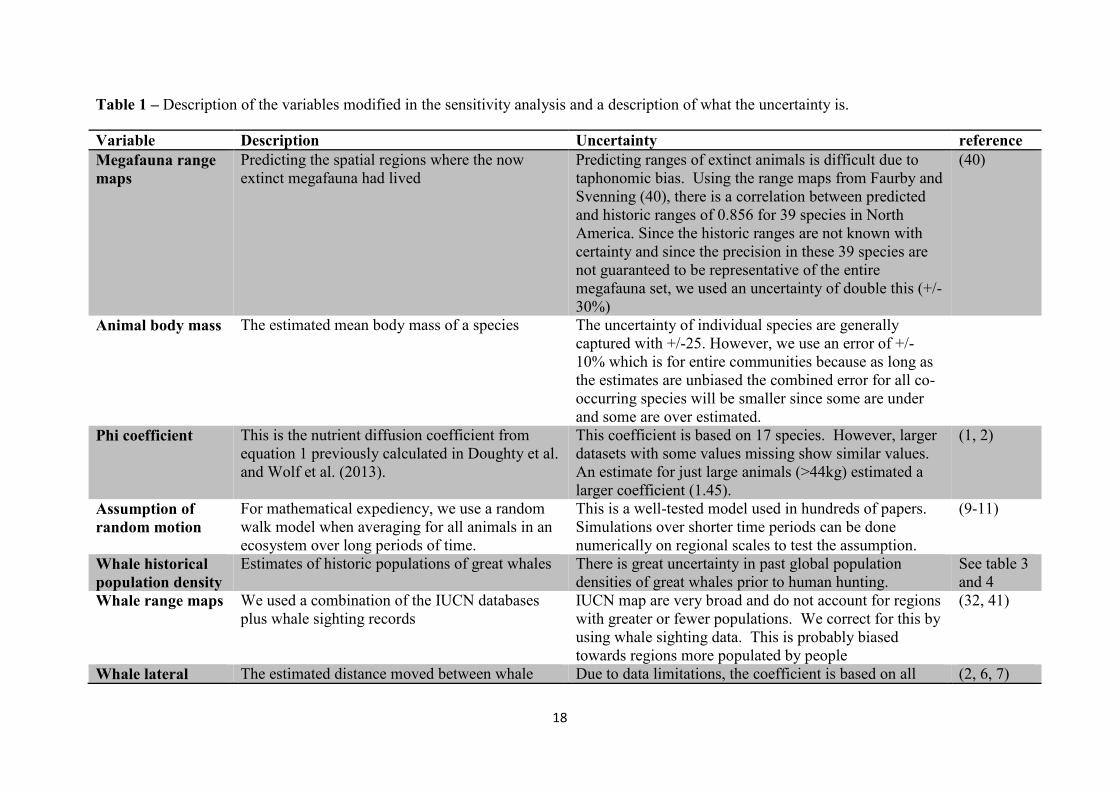
Table 1 – Description of the variables modified in the sensitivity analysis and a description of what the uncertainty is.

Variable Description Uncertainty reference

Megafauna range

maps

Predicting the spatial regions where the now

extinct megafauna had lived

Predicting ranges of extinct animals is difficult due to

taphonomic bias. Using the range maps from Faurby and

Svenning (40), there is a correlation between predicted

and historic ranges of 0.856 for 39 species in North

America. Since the historic ranges are not known with

certainty and since the precision in these 39 species are

not guaranteed to be representative of the entire

megafauna set, we used an uncertainty of double this (+/-

30%)

(40)

Animal body mass The estimated mean body mass of a species The uncertainty of individual species are generally

captured with +/-25. However, we use an error of +/-

10% which is for entire communities because as long as

the estimates are unbiased the combined error for all co-

occurring species will be smaller since some are under

and some are over estimated.

Phi coefficient This is the nutrient diffusion coefficient from

equation 1 previously calculated in Doughty et al.

and Wolf et al. (2013).

This coefficient is based on 17 species. However, larger

datasets with some values missing show similar values.

An estimate for just large animals (>44kg) estimated a

larger coefficient (1.45).

(1, 2)

Assumption of

random motion

For mathematical expediency, we use a random

walk model when averaging for all animals in an

ecosystem over long periods of time.

This is a well-tested model used in hundreds of papers.

Simulations over shorter time periods can be done

numerically on regional scales to test the assumption.

(9-11)

Whale historical

population density

Estimates of historic populations of great whales There is great uncertainty in past global population

densities of great whales prior to human hunting.

See table 3

and 4

Whale range maps We used a combination of the IUCN databases

plus whale sighting records

IUCN map are very broad and do not account for regions

with greater or fewer populations. We correct for this by

using whale sighting data. This is probably biased

towards regions more populated by people

(32, 41)

Whale lateral The estimated distance moved between whale Due to data limitations, the coefficient is based on all (2, 6, 7)

19

diffusion

coefficient

food consumption and defecation based on mean

body size.

mammal data and is not specific to whales. This is likely

a large underestimate, since (7) showed space use for

whales had a much higher exponent than for terrestrial

mammals.

Vertical movement

of nutrients by

marine mammals

Estimate of nutrients moved by deep diving

animals to the surface waters

This term is dependent on estimating population

densities, metabolic rates, and the ratio of food consumed

at depth and defecated in surface waters.

(2)

Seabird range

maps

Estimate of number and spatial area of each

seabird species

IUCN species range maps for seabirds are likely accurate

over land regions, but much less accurate over ocean

regions.

(22)

Seabird food

consumption

Estimate of metabolic consumption and

population density based on mass scaling laws.

These are based on scaling coefficients and are likely

within the 95% confidence interval of the calculated

slope.

(2, 24)

Guano deposition

on land

Estimating the percentage of seabird guano that

arrives on land.

Much guano is defecated at sea versus deposited at

nesting sites. The percentage likely varies widely for

each species. However, we estimate this based on data

from (25, 26).

(25, 26)

Anadromous fish

abundance

Which fish species are anadromous? Where do

they live? What were there historical population

numbers?

The best reference on this (31) details 110 anadromous

fish species, along with 10 other possible ones. This

likely underestimates the total number of anadromous

fish species because it is difficult to estimate. We do not

have species range maps for all of these species and this

is another likely source of underestimation. There is

little data on historical abundances outside of N. America

and Europe. We assume historical abundances

everywhere were similar to N. America and Europe.

(31, 32)

Anadromous fish

nutrient

movement

We use estimates of regional P movement by all

anadromous fish in the Pacific Northwest of the

US from Gresh et al. 2000. This paper quantifies

historical population densities and P contained

within these bodies.

We have no data on mean species size and there is no

data on historical population estimates outside of N.

America and Europe.

(33)

20

21

Table 2 – Values used in our sensitivity analysis: the estimated range in uncertainty, how this

uncertainty was assessed, and a global calculation of the P flux for the low and high estimates.

Expert opinion was estimated by a group of experts (the authors of the paper) of the variable

value in which the group was 95% certain the true value would fall within. If the number is

calculated as a slope, then the 95% confidence interval (1.96*standard error on the slope) is

the potential error.

variable Value

used

Potential

error

estimate

How the

error was

assessed

Past

Global P

flux

Current

Global P

flux

reference

Megafauna

range maps

See

figure 1

±30% for

megafauna

±10% for

current

animals

Expert

opinion

13-23e4

km2 yr

-1

1.1-2.1e4

km2 yr

-1

(40)

Animal body

mass

See (40,

42)

±10% Expert

opinion

16-20e4

km2 yr

-1

1.4-1.9e4

km2 yr

-1

(40, 42)

Phi

coefficient

1.17 ±0.24 Slope

error

3-130e4

km2 yr

-1

0.4-10e4

km2 yr

-1

(2)

Assumption

of random

motion

Random

walk

model

Run model

numerically

Computer

simulation

Simulations

available

upon

request.

Simulations

available

upon

request.

(9-11)

Whale

population

density

See table

4

±50%

historical

±20%

current

Expert

opinion

170-510

million kg

yr-1

64-96

million kg

yr-1

See table

3 and 4

Whale range

maps

See

figure 2

±30%

historical

±10%

current

Expert

opinion

240-310

million kg

yr-1

70-90

million kg

yr-1

(32, 41)

Whale

lateral

diffusion

coefficient

Eq. 1 +30%

-10%

Slope

error and

expert

opinion

5.7 - 8.3e5

km2 yr

-1

2.9-4.2 e4

km2 yr

-1

(2, 6, 7)

Vertical

movement of

nutrients by

marine

mammals

Eq. 2 and

80% of

food

consumed

at depth

moved

vertically

Eq. 2 -

±0.04

65-95%

Slope

error and

expert

opinion

260-430

million kg

yr-1

54-110

million kg

yr-1

(2)

Seabird

range maps

See

Figure 3

±20% Expert

opinion

5-7.6

million kg

yr-1

NA (22)

Seabird food

consumption

Eq. 2 and

3

Eq. 2 -

±0.04

Slope

error

3-9 million

kg yr-1

NA (2, 24)

22

Eq. 3 -

±0.10

Guano

deposition

on land

20% 5-50% Slope

error and

expert

opinion

1.5-16

million kg

yr-1

NA (25, 26)

Anadromous

fish

abundance

See

figure 3

+200%

-50%

Slope

error and

expert

opinion

71-430

million kg

yr-1

3-16

million kg

yr-1

(31, 32)

Anadromous

fish nutrient

movement

Scaling

results

from

Gresh et

al. 2000

+100%

-50%

Expert

opinion

71-280

million kg

yr-1

3-12

million kg

yr-1

(33)

23

Table 3 – Data table used to calculate lateral nutrient distribution capacity of great whales in oceans. Numbers are in thousands. NA is the

North Atlantic, NP is the North Pacific, SH is the Southern Ocean. Unless otherwise stated all data references are from Christensen 2006 (43).

Estimating past populations of animals has inherent large uncertainties due to poor historical data. Numbers with especially high uncertainty are

listed as a range with a footnote below explaining the possible discrepancy from Christensen 2006 (43). Due to the large uncertainty in these

numbers, in a sensitivity study, we estimate the uncertainty of our estimates at 30% (SI appendix Table 2).

Species Pre NA Pre NP Pre SH Pre

Other

2001 NA 2001 NP 2001

SH

2001

Other

Reference

Balaenoptera

borealis 10.6 68.4 167 0 7 14.7 27.4 0

Physeter

macrocephalus 0 0 0 1110 0 0 0 360

Global populations from

(44)

Balaenoptera

physalus 73 65 625 0 56 31 23 0

Eschrichtius

robustus 0 25 0 0 0 16 0 0

Balaenoptera

musculus 7.5 6 256-327*1

0 0.4 3 1-3*2

0

Balaenoptera

brydei 0 52 94 0 0 41 91 0

Christensen and IUCN

Red List

Megaptera

novaeangliae

112 20 140-199*3

0 20 20

22.5-

40*4

0

Estimates for pre-NA

from (45); estimates for

contemporary

humpbacks in NP from

(46), pre NP #s have

been rounded up to

reflect this increase

Balaenoptera

acutorostrata 211 47 379 0 157 32 318 0

Balaenoptera 211 47 379 0 157 32 318 0

24

bonaerensis

Eubalaena

glacialis 14 0 0 0 0.4 0 0 0

Eubalaena

australis 0 0 70-86*5

0 0 0

10-

12*6

0

Eubalaena

japonica 0 31.75 0 0 0 0.4 0 0

(47)

Balaena

mysticetus 0 0 0 89 0 0 0 9

*3Estimated population for Antarctic blue whales could be 256,000.

*4For Antarctic blue whales in 1997 the population was 2,300 individuals. If one projects that to 2001 given the estimated growth rate for this

population (6.4%/year as agreed by the IWC), one gets an abundance of 3,000.

*3In the Southern Hemisphere, Humpback whales estimated pre-exploitation abundance (K) is 140,000 given the IWC most recent assessments.

*4The most recent abundance estimate for all whales combined is 80,000 in 2010. It is hard to extrapolate back to 2001 (which is the year shown

in the table), but a crude calculation indicates the 2001 abundance would have been at least 40,000 whales.

*5The IWC estimated populations at about 70,000 whales under the assumption of an intrinsic growth rate of 7%/year (which is consistent with

the three major right whale breeding populations).

*6The abundance of Southern Right Whales in 2001 projected from the IWC assessments is 10,000.

25

Table 4 – Data table used to calculate vertical nutrient distribution by marine mammals. Dive depths are from Ponganis 2011 (18).

Population sizes are from Christensen 2006 (43) unless otherwise stated.

Species

Pre

NA

Pre

NP

Pre

SH

Pre

Other

2001

NA

2001

NP

2001

SH

2001

Other

weight Diving

depth

reference

Cystophora cristata 700 0 0 0 70 0 0 0

200 100-

600

IUCN Red

List

Globicephala

macrorhynchus 33 624 0 0 33 624 0 0

2000 100-

800

IUCN Red

List

Hyperoodon

ampullatus 58 0 0 0 49 0 0 0

6500

800

Globicephala melas 871 0 0 0 795 0 0 0

2500 100-

800

Phocarctos hookeri 0 0 120 0 0 0 12 0

400

NaN

Pre hunting

estimates

are based

on range

reduction

Mirounga

angustirostris 0 200 0 0 0 200 0 0

2000

437

Mirounga leonine 0 0 1000 0 0 0 650 0

2000 269-

552

Iucn Red

List

Physeter

microcephalus 0 0 0 1110 0 0 0 360

14000

400-

900

Global

populations

from (44)

Balaenoptera

physalus 7.5 6 327 0 0.4 3 1 0

150000 180-

200

Ziphius cavirostros 0 97 0 100 0 97 0 100

2500 1070-

1334

Leptonychotes 0 0 500 0 0 0 500 0 500 150-

26

weddelli 400

27

Table 5 – Species list of anadromous fish from(31), species used in our estimates (if no

species range map was available, we used a similar species from the same genus), the

status is the certainty of if the fish were anadromous (maybe is not certain, and blank is

more certain), and the estimated pixel area (in km2) occupied by the species which

includes both the land and river area within the pixel.

Anadromous fish species used status estimated area

(km2)

Acipenser baerii Acipenser baerii 1.01E+05

Acipenser brevirostrum Acipenser brevirostrum 9.06E+05

Acipenser fulvescens Acipenser fulvescens maybe 5.61E+06

Acipenser gueldenstaedtii Acipenser

gueldenstaedtii

maybe 3.41E+06

Acipenser medirostris Acipenser medirostris 6.01E+05

Acipenser nudiventris Acipenser nudiventris maybe 2.04E+06

Acipenser oxyrinchus Acipenser oxyrinchus 2.45E+06

Acipenser ruthenus Acipenser ruthenus 4.17E+06

Acipenser stellatus Acipenser stellatus 3.48E+06

Acipenser sturio Acipenser sturio 4.26E+06

Acipenser transmontanus Acipenser

transmontanus

maybe 1.21E+06

Acipenser usohuso NaN 0.00E+00

28

Alosa aestivalis Alosa aestivalis 1.02E+06

Alosa alabamae Alosa alabamae 8.97E+05

Alosa caspia Alosa caspia 1.07E+06

Alosa chrysochloris Alosa tanaica 2.94E+05

Alosa fallax Alosa fallax 2.99E+06

Alosa kessleri Alosa kessleri 1.15E+06

Alosa mediocris Alosa mediocris 6.88E+05

Alosa pontica Alosa volgensis 8.39E+05

Alosa pseudoharengus Alosa pseudoharengus 2.25E+06

Alosa sapidissima Alosa sapidissima 1.97E+06

Anchoviella

lepidentostole

NaN 0.00E+00

Anodontostoma

chacunda

NaN 0.00E+00

Arius felis Arius arius 1.94E+06

Arius heudeloti Arius uncinatus 4.62E+04

Arius militaris Arius acutirostris 2.59E+05

Arius graeffei Arius gagora 1.54E+05

Arius latiscutatus Arius gigas 1.80E+06

Arius madagascariensis Arius madagascariensis 1.18E+05

Batanga lebretonis NaN 0.00E+00

Clupanodon

thrischacunda

Clupeonella caspia 5.59E+05

Clupeonella cultiventris Clupeonella caspia 5.59E+05

Coregonus albula Coregonus albula 2.70E+06

Coregonus artedii Coregonus alpinus maybe 6.63E+03

29

Coregonus artedii Coregonus autumnalis 6.76E+06

Coregonus autumnalis Coregonus baerii 1.63E+05

Coregonus canadensis Coregonus lavaretus maybe 2.01E+04

Coregonus clupeaformis Coregonus nasus 8.14E+06

Coregonus laurettae Coregonus oxyrinchus 1.19E+05

Coregonus lavaretus Coregonus megalops 2.02E+05

Coregonus muskun Coregonus peled 4.50E+06

Coregonus nasus Coregonus reighardi 3.09E+05

Coregonus oxyrinchus Coregonus vandesius maybe 4.42E+04

Coregonus ussuriensis Coregonus zenithicus maybe 1.56E+06

Dormitator latifrons Dormitator lebretonis 2.53E+06

Dormitator maculatus NaN 0.00E+00

Dorosoma cepedianum Dorosoma cepedianum 5.52E+06

Dorosoma petenense Dorosoma petenense 1.62E+06

Eleotris pisonis Eleotris oxycephala 2.22E+06

Gasterosteus aculeatus Gasterosteus aculeatus 9.70E+06

Geotria Australis Geotria australis 1.82E+06

30

Hemisalanx prognathus NaN maybe 0.00E+00

Herkotslichthys gotoi NaN 0.00E+00

Herkotslichthys

koningsbergeri

NaN 0.00E+00

Hucho perryi Hucho hucho 3.55E+05

Hypomesus

transpacificus

Hypomesus olidus 1.66E+07

Hypomesus olidus Hypomesus transpacificus 1.06E+05

Ilisha novalcula Ilisha novacula 8.56E+05

Ilisha africana NaN 0.00E+00

Ilisha megaloptera NaN 0.00E+00

Lampetra japonica Lampetra aepyptera 1.30E+06

Lampetra wagneri Lampetra hubbsi 2.31E+05

Lampetra tridentata Lampetra richardsoni 8.01E+05

Lampetra ayresii Lampetra ayresii 6.69E+05

Lampetra fluviatilis Lampetra planeri 3.72E+06

Lampetra tridentata Lampetra ninae 4.22E+04

Lepisosteus osseus Lepisosteus osseus 4.99E+06

31

Leucopsarion petersi NaN 0.00E+00

Lovettia seali NaN 0.00E+00

Lycengraulis olidus NaN 0.00E+00

Lycengraulis simulator NaN 0.00E+00

Microgadus tomcod Microgadus tomcod 1.68E+05

Microphis brachyurus Microphis brachyurus 2.35E+05

Mordacia mordax NaN 0.00E+00

Morone saxatilis Morone saxatilis 1.63E+06

Morone americanus Morone americana 1.19E+06

Nematalosa vlaminghi NaN 0.00E+00

Nematalosa galatheae NaN 0.00E+00

Neosalanx jordani Neosalanx

brevirostris

maybe 2.53E+06

Oncorhynchus gilae Oncorhynchus gilae maybe 2.01E+05

Oncorhynchus nerka Oncorhynchus nerka maybe 2.62E+06

Oncorhynchus

tshawytscha

NaN 0.00E+00

Oncorhynchus keta NaN 0.00E+00

Oncorhynchus kisutch NaN 0.00E+00

Oncorhynchus masou NaN 0.00E+00

Osmerus mordax Osmerus mordax 4.26E+06

Osmerus eperlanus Osmerus eperlanus 2.63E+06

32

Pellona ditcheli Pellonula vorax 1.83E+06

Pellonula leonensis NaN 0.00E+00

Pellonula vorax NaN 0.00E+00

Petromyzon marinus Petromyzon marinus 4.34E+06

Prosopium cylindraceum Protosalanx chinensis 1.25E+06

Protosalanx chinensis NaN 2.17E+07

Protosalanx

hyalocranium

NaN maybe 0.00E+00

Pungitius pungitius Pungitius pungitius 0.00E+00

Retropinna retropinna Retropinna retropinna 4.81E+05

Retropinna tasmanica NaN 0.00E+00

Retropinna semoni NaN 0.00E+00

Salangichthys microdon NaN 0.00E+00

Salangichthys ishikawae NaN 0.00E+00

Salanx ariakensis Salanx chinensis 4.62E+05

Salanx cuvieri Salanx cuvieri maybe 2.65E+05

Salanx acuticeps NaN maybe 0.00E+00

Salmo salar Salmo salar 2.12E+06

Salmo trutta Salmo trutta 1.01E+07

Salmo gairdneri Salmo macrostigma 3.68E+05

Salmo clarki Salmo labrax 2.34E+06

Salmo penshinensis Salmo platycephalus 5.25E+04

33

Salvelinus alpinus Salvelinus alpinus 1.22E+07

Salvelinus fontinalis Salvelinus umbla 1.71E+05

Salvelinus malma Salvelinus murta 4.15E+03

Salvelinus leucomaenis Salvelinus inframundus 6.14E+04

Salvelinus confluentis Salvelinus confluentus 2.63E+06

Spirinchus lanceolatus Spirinchus thaleichthys 5.37E+05

Spirinchus thaleichthys NaN 0.00E+00

Sokellia anisodon Stokellia anisodon 6.82E+04

Strongylura kreffti Strongylura marina 1.25E+06

Tenualosa ilisha Tenualosa ilisha 2.40E+06

Tenualosa macrura Tenualosa thibaudeaui 2.61E+05

Tenualosa reevesi NaN 0.00E+00

Tenualosa toli NaN 0.00E+00

34

References

1. Doughty CE, Wolf A, & Malhi Y (2013) The legacy of the Pleistocene megafauna extinctions on nutrient availability in Amazonia. Nat Geosci 6(9):761-764.

2. Wolf A, Doughty CE, & Malhi Y (2013) Lateral Diffusion of Nutrients by Mammalian Herbivores in Terrestrial Ecosystems. Plos One 8(8).

3. Faurby S & Svenning JC (2015) A species-level phylogeny of all extant and late Quaternary extinct mammals using a novel heuristic-hierarchical Bayesian approach. Mol Phylogenet Evol.

4. Mosbrugger V & Utescher T (1997) The coexistence approach - a method for quantitative reconstructions of Tertiary terrestrial palaeoclimate data using plant fossils. Palaeogeogr Palaeocl 134(1-4):61-86.

5. Wolff WJ (2000) The south-eastern North Sea: losses of vertebrate fauna during the past 2000 years. Biol Conserv 95(2):209-217.

6. Tershy BR (1992) Body Size, Diet, Habitat Use, and Social-Behavior of Balaenoptera Whales in the Gulf of California. J Mammal 73(3):477-486.

7. McCauley DL, et al. (2015) Marine defaunation: Animal loss in the global ocean. Science. 8. Berg HC (1993) Random Walks in Biology. (Princeton.). 9. Okubo A & Levin SA (2001) Diffusion and ecological problems : modern perspectives

(Springer, New York) 2nd Ed pp xx, 467 p. 10. Ovaskainen O & Crone EE (2009) Modeling animal movement with diffusion. Spatial Ecology,

Chapman & Hall/CRC Mathematical & Computational Biology, (Chapman and Hall/CRC), pp 63-83.

11. Skellam JG (1951) Random Dispersal in Theoretical Populations. Biometrika 38(1-2):196-218. 12. Ilse LM & Hellgren EC (1995) Resource Partitioning in Sympatric Populations of Collared

Peccaries and Feral Hogs in Southern Texas. J Mammal 76(3):784-799. 13. Augustine DJ & McNaughton SJ (1998) Ungulate effects on the functional species

composition of plant communities: Herbivore selectivity and plant tolerance. J Wildlife Manage 62(4):1165-1183.

14. Mcnaughton SJ (1988) Mineral-Nutrition and Spatial Concentrations of African Ungulates. Nature 334(6180):343-345.

15. White KAJ, Lewis MA, & Murray JD (1996) A model for wolf-pack territory formation and maintenance. J Theor Biol 178(1):29-43.

16. Rees PA (1982) Gross Assimilation Efficiency and Food Passage Time in the African Elephant. African Journal of Ecology 20(3):193-198.

17. Elser JJ, Dobberfuhl, D.R., MacKay, N.A., Schampel, J.H. (1996) Organism Size , Life History, and N:P Stoichiometry. Toward a unified view of cellular and ecosystem processes. BioScience 46(9).

18. Ponganis PJ (2011) Diving mammals. Comprehensive Physiology 1:517-535. 19. Alcaraz M, et al. (2014) Changes in the C, N, and P cycles by the predicted salps-krill shift in

the southern ocean. frontiers in marine science. 20. Roman J & McCarthy JJ (2010) The Whale Pump: Marine Mammals Enhance Primary

Productivity in a Coastal Basin. Plos One 5(10). 21. Ratnarajah L, Bowie AR, Lannuzel D, Meiners KM, & Nicol S (2015) The Biogeochemical Role

of Baleen Whales and Krill in Southern Ocean Nutrient Cycling (vol 9, e114067, 2014). Plos One 10(4).

22. NatureServe BIa (2014) Bird species distribution maps of the world. . BirdLife International, Cambridge, UK and NatureServe, Arlington, USA.

23. Dunning JB (2007) Handbook of Avian Body Masses. Second edition. 24. Juanes F (1986) Population-Density and Body Size in Birds. Am Nat 128(6):921-929.

35

25. Anderson WB & Polis GA (1999) Nutrient fluxes from water to land: seabirds affect plant nutrient status on Gulf of California islands. Oecologia 118(3):324-332.

26. Mulder CPH, et al. (2011) Impacts of Seabirds on Plant and Soil Properties. Seabird Islands: Ecology, Invasion, and Restoration, ed Christa P. H. Mulder WBA, David R. Towns, and Peter J. Bellingham).

27. Pennycuick CJ, Croxall JP, & Prince PA (1984) Scaling of Foraging Radius and Growth-Rate in Petrels and Albatrosses (Procellariiformes). Ornis Scand 15(3):145-154.

28. Jackson S (1992) Do Seabird Gut Sizes and Mean Retention Times Reflect Adaptation to Diet and Foraging Method. Physiol Zool 65(3):674-697.

29. Schneider DC (2002) Scaling theory: Application to marine ornithology. Ecosystems 5(8):736-748.

30. Buendia C, Kleidon A, & Porporato A (2010) The role of tectonic uplift, climate, and vegetation in the long-term terrestrial phosphorous cycle. Biogeosciences 7(6):2025-2038.

31. McDowall RM (1988) Diadromy in Fishes: Migrations between Freshwater and Marine Environments (Croom Helm, London).

32. IUCN (2010) IUCN Red List of Threatened Species. Version 2010.4. 33. Gresh T, Lichatowich J, & Schoonmaker P (2000) An estimation of historic and current levels

of salmon production in the Northeast Pacific ecosystem: Evidence of a nutrient deficit in the freshwater systems of the Pacific Northwest. Fisheries 25(1):15-21.

34. de Groot SJ (2002) A review of the past and present status of anadromous fish species in the Netherlands: is restocking the Rhine feasible? Ecological Restoration of Aquatic and Semi-Aquatic Ecosystems in the Netherlands (NW Europe). Developments in Hydrobiology 166:205-218.

35. Limburg KE & Waldman JR (2009) Dramatic Declines in North Atlantic Diadromous Fishes. Bioscience 59(11):955-965.

36. Beaulaton L, Taverny C, & Castelnaud G (2008) Fishing, abundance and life history traits of the anadromous sea lamprey (Petromyzon marinus) in Europe. Fish Res 92(1):90-101.

37. Rochard E, Castelnaud G, & Lepage M (1990) Sturgeons (Pisces, Acipenseridae) - Threats and Prospects. J Fish Biol 37:123-132.

38. Damuth J (2007) A macroevolutionary explanation for energy equivalence in the scaling of body size and population density. Am Nat 169(5):621-631.

39. Estes JA, et al. (2011) Trophic Downgrading of Planet Earth. Science 333(6040):301-306. 40. Faurby S & Svenning JC (2015) Historic and prehistoric human-driven extinctions have

reshaped global mammal diversity patterns. P Roy Soc B-Biol Sci. 41. seamap ((http://seamap.env.duke.edu/). 42. Smith FA, et al. (2003) Body mass of late quaternary mammals. Ecology 84(12):3403-3403. 43. Christensen LB (2006) Marine Mammal Populations: Reconstructing historical abundances at

the global scale. Fisheries Centre Research Reports 14(9). 44. Whitehead H (2002) Estimates of current global population size and historical trajectory for

sperm whales. Mar Ecol Progr Ser 242:295-304. 45. Ruegg KC, et al. (2013) Long-term population size of the North Atlantic humpback whale

within the context of worldwide population structure. Conserv. Genet. 14:104-114. 46. Calambokidis Jea (2008) SPLASH: Structure of Populations, Levels of Abundance and Status

of Humpback Whales in the North Pacific (U.S. Dept of Commerce). 47. Croll DA, Kudela R, & Tershy BR (2006) Ecosystem impacts of the decline of large whales in

the North Pacific. Whales, whaling and ocean ecosystems., ed Estes JA DD, Doak DF, Williams TM, Brownell Jr. RL (University of California Press., Berkeley).

36