glob

March 2009

Volume I

Issue 3

SPPI Monthly CO2Report

Christopher Monckton, Editor

2

7 years’ global cooling on all measures

CO2 concentration is rising, but still well below IPCC predictions

IPCC predicts rapid, exponential CO2 growth that is not occurring

The 29-year global warming trend is just 2.5 °F (1.5 °C) per century

A long, fast decline: 7 years’ global cooling at 3.6 °F (2 °C) / century

All global surface temperature datasets show seven years’ cooling

Sea level: the “Armageddon scenario” is not occurring

Arctic sea-ice extent has scarcely declined in the 29 years since 1980

Antarctic sea-ice extent reached a 30-year peak in late 2007

The regular “heartbeat” of global sea-ice extent: steady for 30 years

Hurricane, typhoon, & tropical cyclone activity are at a record low

Proof that CO2’s warming effect is exaggerated

Your climate-sensitivity ready reckoner

New Science

Contents

3

7 years’ global cooling on all measuresSPPI’s authoritative Monthly CO2 Report for March 2009 demonstrates that all global-temperature datasetsshow rapid global cooling for seven full years, at a rate equivalent to 2 C° (3.6 F°) per century. Main points –

Since Al Gore’s climate movie An Inconvenient Truth was launched in January 2005, global cooling has occurred at theequivalent of 10 °F (5.5 °C) per century. If this rapid cooling were to continue, the Earth would be in an Ice Age by 2100.

The UN’s climate panel, the IPCC, had projected temperature increases at 4.5 to 9.5 °F (2.4 to 5.3 °C) per century, with acentral estimate of 7 °F (3.9 °C) per century. None of the IPCC’s computer models had predicted a prolonged cooling.

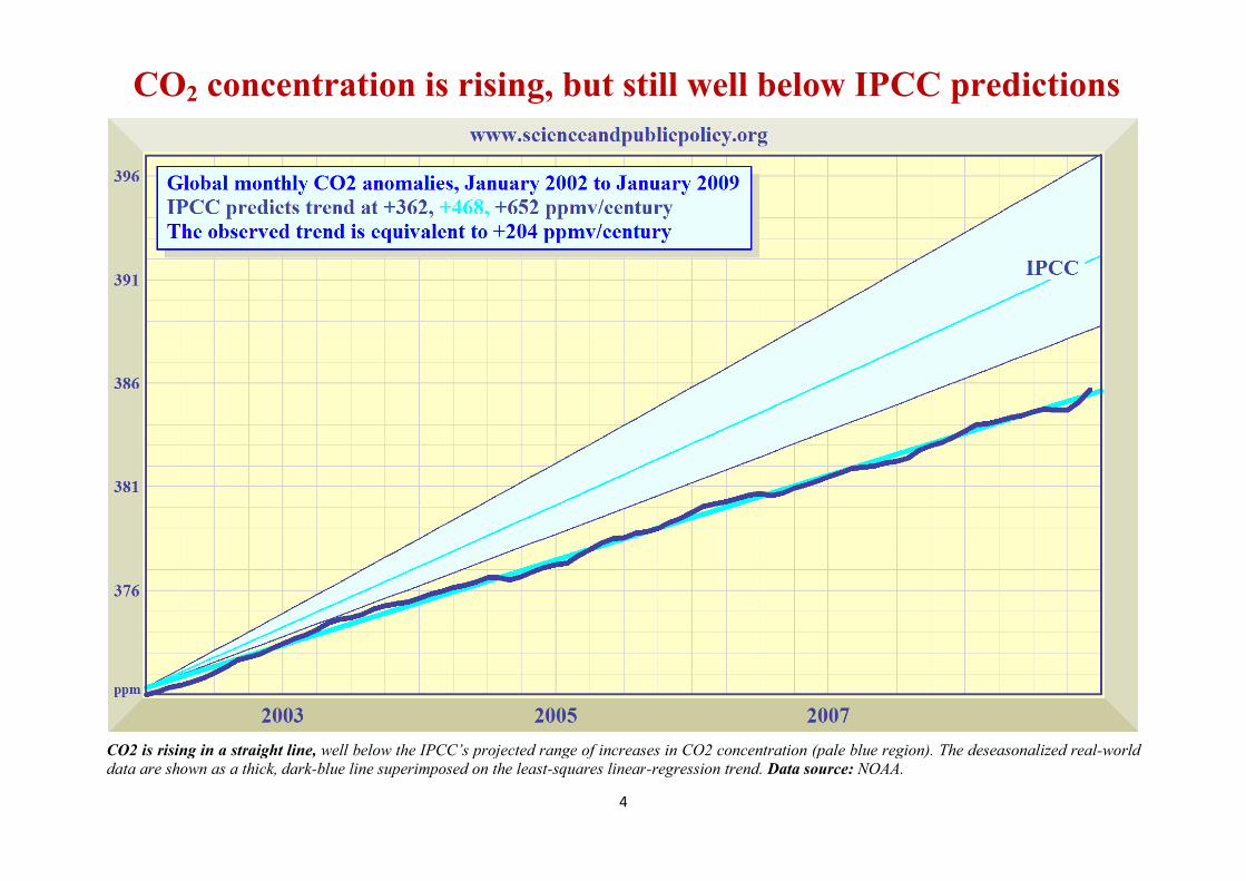
The IPCC’s estimates of growth in atmospheric CO2 concentration are excessive. They assume CO2 concentration willrise exponentially from today’s 385 parts per million to reach 730 to 1020 ppm, central estimate 836 ppm, by 2100.

However, for seven years, CO2 concentration has been rising in a straight line towards just 575 ppmv by 2100. This alonehalves the IPCC’s temperature projections. Since 1980 temperature has risen at only 2.5 °F (1.5 °C) per century.

Sea level rose just 8 inches in the 20th century and has been rising at just 1 ft/century since 1993. Though James Hansen ofNASA says sea level will rise 246 feet, sea level has scarcely risen since the beginning of 2006.

Sea ice extent in the Arctic has now recovered to the 30-year average. In the Antarctic, sea ice extent reached a record highlate in 2007, and has remained plentiful since. Global sea ice extent shows little trend for 30 years.

The Accumulated Cyclone Energy Index is a 24-month running sum of monthly energy levels in all hurricanes,typhoons and tropical cyclones. The Index shows that at present there is less severe tropical-storm activity thanat any time in 30 years.

Satellite measurements prove that official predictions overestimate CO2’s effect on temperature 15-fold.

SPPI Monthly CO2 Report : : March 2009Accurate, Authoritative Analysis for Today’s Policymakers

4

CO2 concentration is rising, but still well below IPCC predictions

CO2 is rising in a straight line, well below the IPCC’s projected range of increases in CO2 concentration (pale blue region). The deseasonalized real-worlddata are shown as a thick, dark-blue line superimposed on the least-squares linear-regression trend. Data source: NOAA.

5

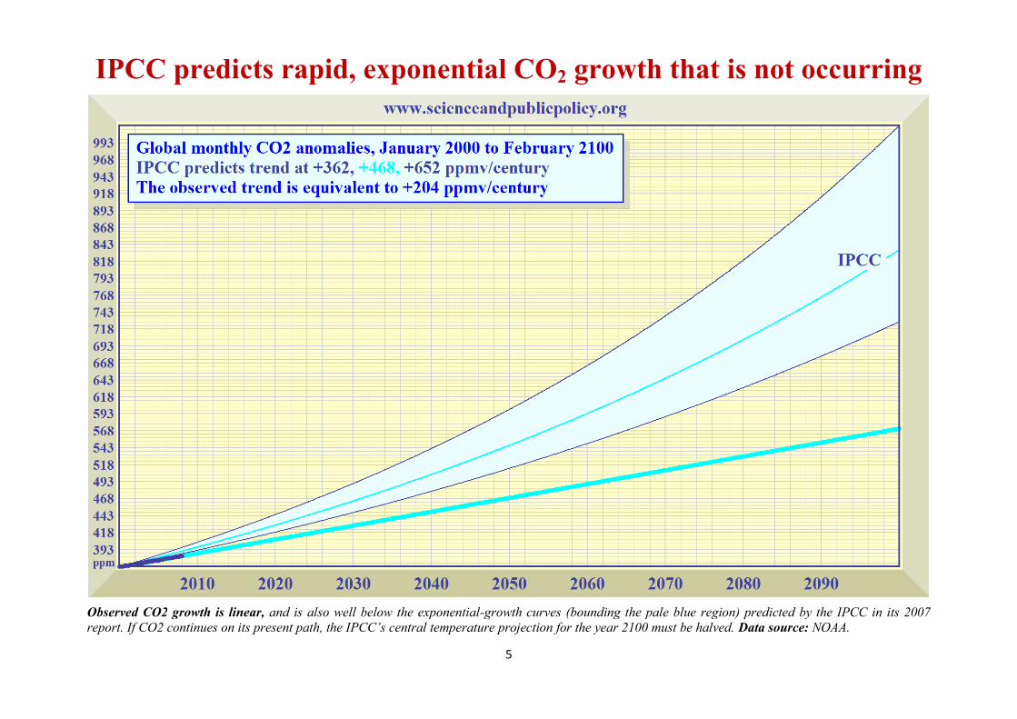
IPCC predicts rapid, exponential CO2 growth that is not occurring

Observed CO2 growth is linear, and is also well below the exponential-growth curves (bounding the pale blue region) predicted by the IPCC in its 2007report. If CO2 continues on its present path, the IPCC’s central temperature projection for the year 2100 must be halved. Data source: NOAA.

6

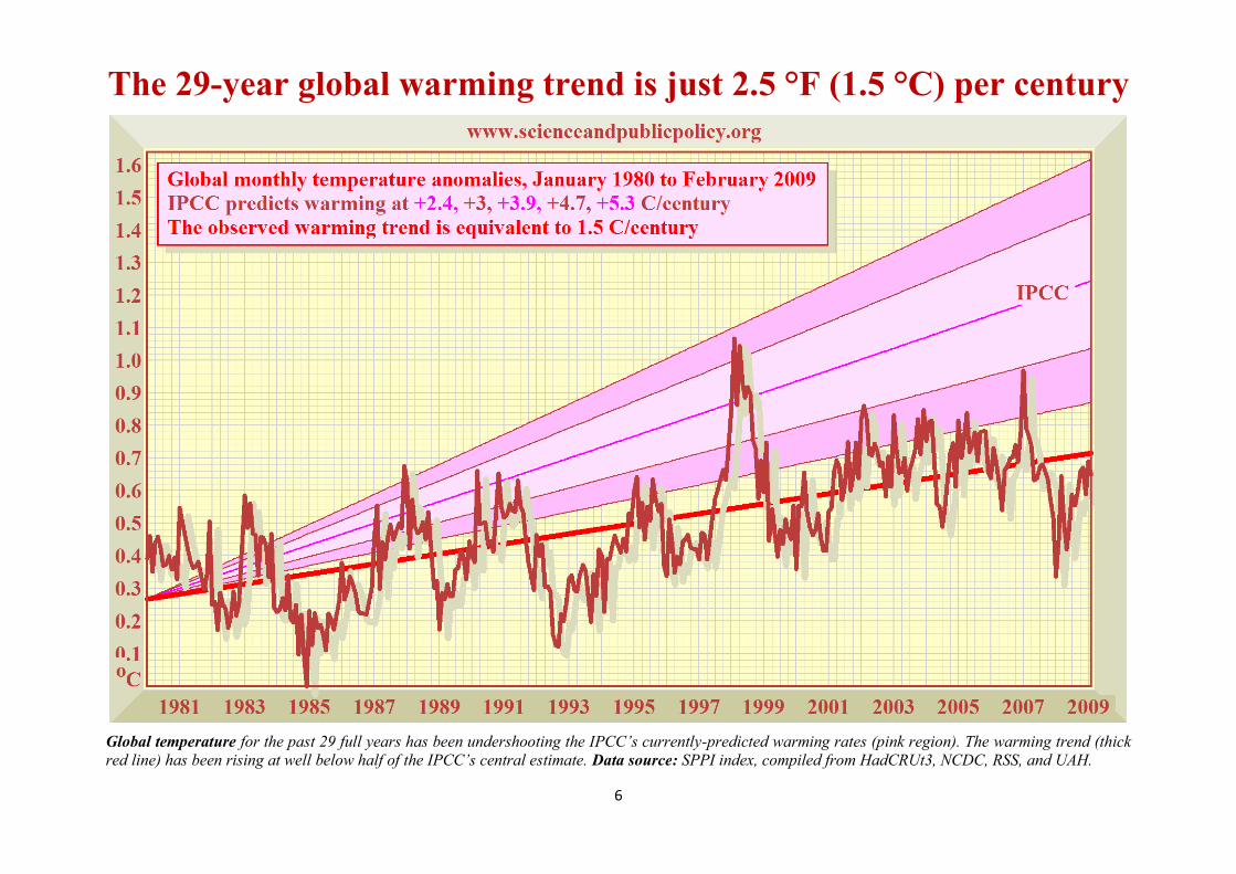
The 29-year global warming trend is just 2.5 °F (1.5 °C) per century

Global temperature for the past 29 full years has been undershooting the IPCC’s currently-predicted warming rates (pink region). The warming trend (thickred line) has been rising at well below half of the IPCC’s central estimate. Data source: SPPI index, compiled from HadCRUt3, NCDC, RSS, and UAH.

7

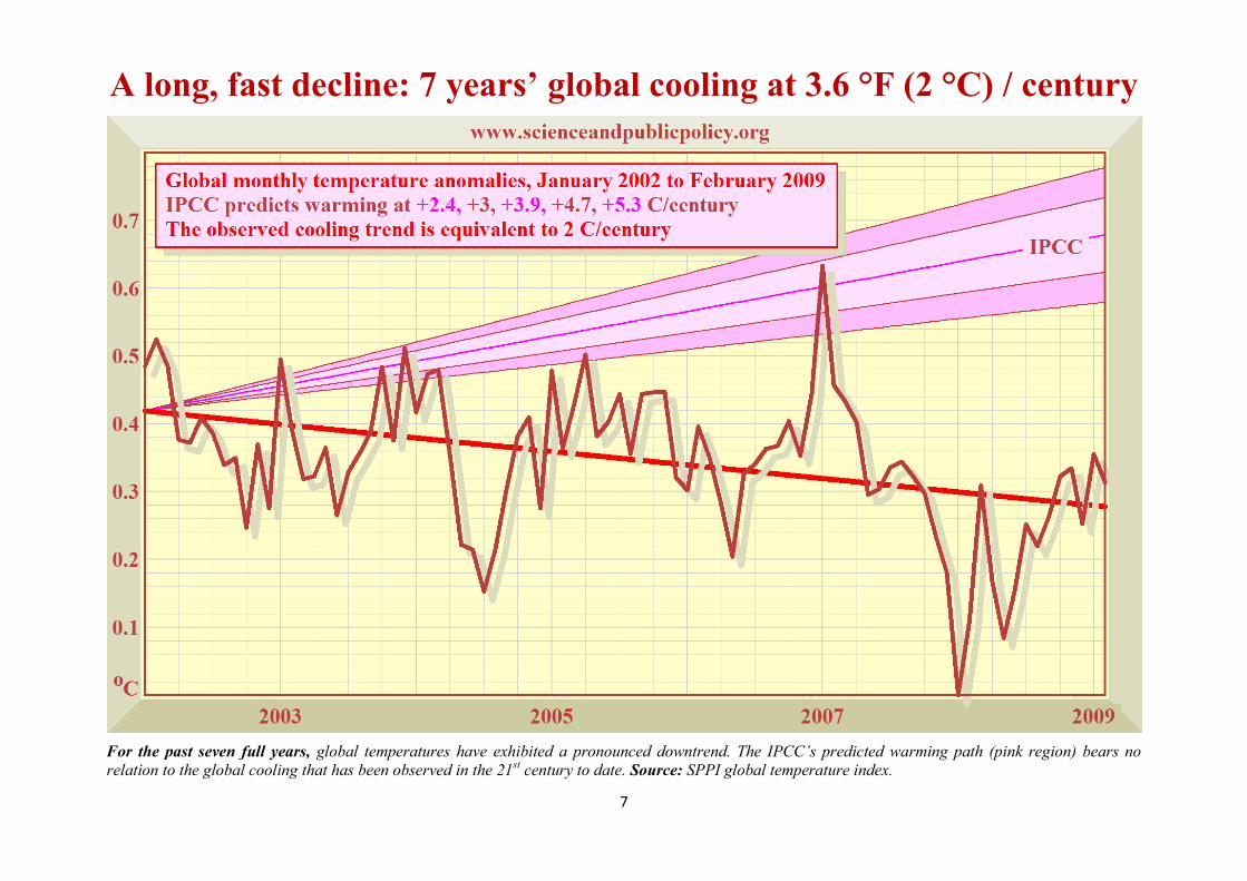
A long, fast decline: 7 years’ global cooling at 3.6 °F (2 °C) / century

For the past seven full years, global temperatures have exhibited a pronounced downtrend. The IPCC’s predicted warming path (pink region) bears norelation to the global cooling that has been observed in the 21st century to date. Source: SPPI global temperature index.

8

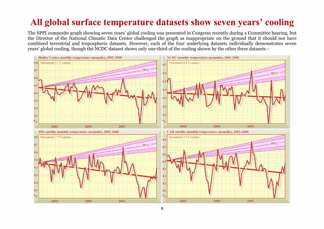
All global surface temperature datasets show seven years’ coolingThe SPPI composite graph showing seven years’ global cooling was presented in Congress recently during a Committee hearing, butthe Director of the National Climatic Data Center challenged the graph as inappropriate on the ground that it should not havecombined terrestrial and tropospheric datasets. However, each of the four underlying datasets individually demonstrates sevenyears’ global cooling, though the NCDC dataset shows only one-third of the cooling shown by the other three datasets –

9

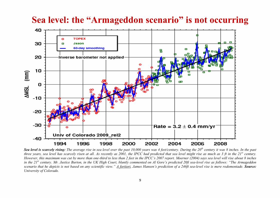
Sea level: the “Armageddon scenario” is not occurring

Sea level is scarcely rising: The average rise in sea level over the past 10,000 years was 4 feet/century. During the 20th century it was 8 inches. In the pastthree years, sea level has scarcely risen at all. As recently as 2001, the IPCC had predicted that sea level might rise as much as 3 ft in the 21st century.However, this maximum was cut by more than one-third to less than 2 feet in the IPCC’s 2007 report. Moerner (2004) says sea level will rise about 8 inchesin the 21st century. Mr. Justice Burton, in the UK High Court, bluntly commented on Al Gore’s predicted 20ft sea-level rise as follows: “The Armageddonscenario that he depicts is not based on any scientific view.” A fortiori, James Hansen’s prediction of a 246ft sea-level rise is mere rodomontade. Source:University of Colorado.

10

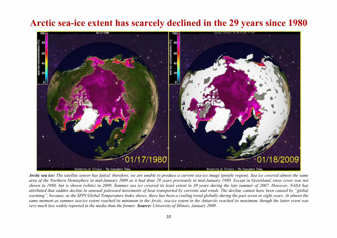
Arctic sea-ice extent has scarcely declined in the 29 years since 1980

Arctic sea ice: The satellite sensor has failed: therefore, we are unable to produce a current sea-ice image (purple region). Sea ice covered almost the samearea of the Northern Hemisphere in mid-January 2009 as it had done 29 years previously in mid-January 1980. Except in Greenland, snow cover was notshown in 1980, but is shown (white) in 2009. Summer sea ice covered its least extent in 30 years during the late summer of 2007. However, NASA hasattributed that sudden decline to unusual poleward movements of heat transported by currents and winds. The decline cannot have been caused by “globalwarming”, because, as the SPPI Global Temperature Index shows, there has been a cooling trend globally during the past seven or eight years. At almost thesame moment as summer sea-ice extent reached its minimum in the Arctic, sea-ice extent in the Antarctic reached its maximum, though the latter event wasvery much less widely reported in the media than the former. Source: University of Illinois, January 2009.

11

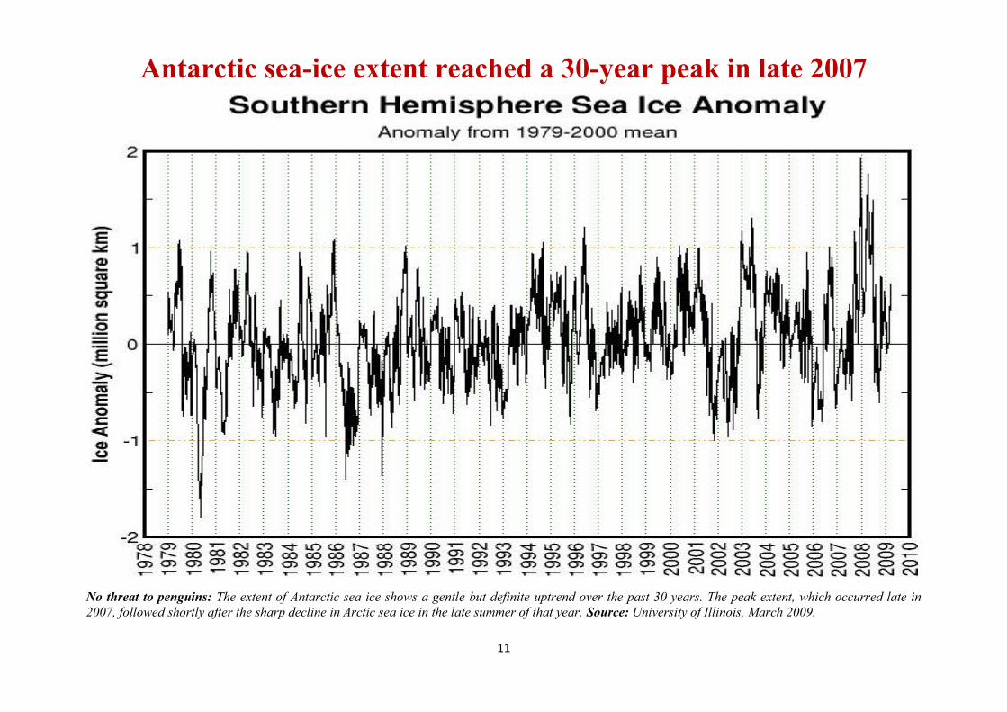
Antarctic sea-ice extent reached a 30-year peak in late 2007

No threat to penguins: The extent of Antarctic sea ice shows a gentle but definite uptrend over the past 30 years. The peak extent, which occurred late in2007, followed shortly after the sharp decline in Arctic sea ice in the late summer of that year. Source: University of Illinois, March 2009.

12

The regular “heartbeat” of global sea-ice extent: steady for 30 years

Planetary “cardiogram”: There has been a very slight decline in the trend (red) of global sea-ice extent over the decades, chiefly attributable to loss of seaice in the Arctic during the summer, which was well below the mean in 2007, with some recovery in 2008. However, the 2008 peak sea-ice extent was exactlyon the 1979-2000 mean, and current sea-ice extent is also on the 1979-2000 mean. The decline in summer sea-ice extent in the Arctic, reflected in the globalsea-ice anomalies over most of the past eight years, runs counter to the pronounced global atmospheric cooling trend over the same period, suggesting thatthe cause of the regional sea-ice loss cannot have been “global warming”. Seabed volcanic activity recently reported in the Greenland/Iceland gap, withseabed temperatures of up to 574 °F, may have contributed to the loss of Arctic sea-ice. Source: University of Illinois, March 2009.

13

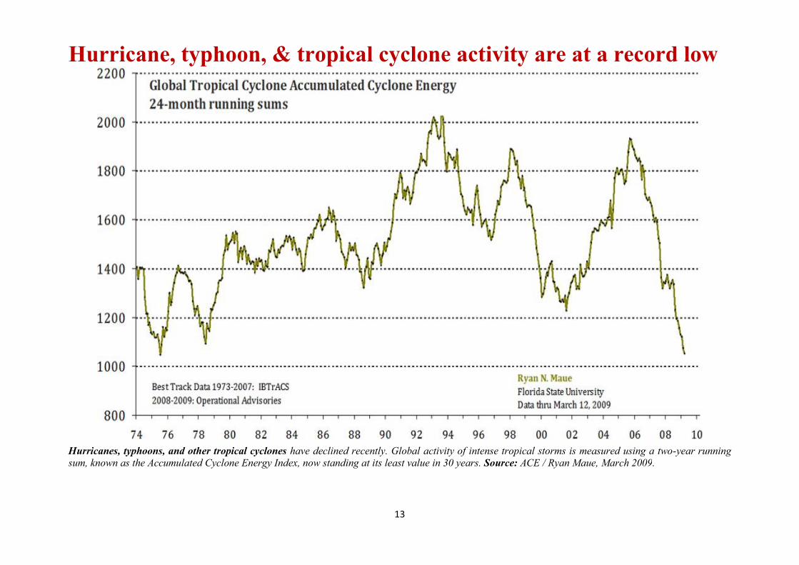
Hurricane, typhoon, & tropical cyclone activity are at a record low

Hurricanes, typhoons, and other tropical cyclones have declined recently. Global activity of intense tropical storms is measured using a two-year runningsum, known as the Accumulated Cyclone Energy Index, now standing at its least value in 30 years. Source: ACE / Ryan Maue, March 2009.

14

Proof that CO2’s warming effect is exaggeratedAST MONTH Science Focus calculated that the UN had approximately (and perhaps inadvertently) doubled the value ofeach of four parameters, and had then multiplied them together, causing a 15-fold exaggeration of the anthropogenicincrease in global surface temperature. This month, with grateful acknowledgement to Professor Richard Lindzen, we

provide real-world confirmation of our theoretically-calculated conclusion.

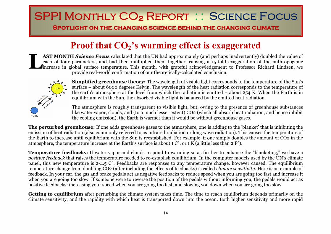
Simplified greenhouse theory: The wavelength of visible light corresponds to the temperature of the Sun’ssurface – about 6000 degrees Kelvin. The wavelength of the heat radiation corresponds to the temperature ofthe earth’s atmosphere at the level from which the radiation is emitted – about 254 K. When the Earth is inequilibrium with the Sun, the absorbed visible light is balanced by the emitted heat radiation.

The atmosphere is roughly transparent to visible light, but, owing to the presence of greenhouse substanceslike water vapor, clouds, and (to a much lesser extent) CO2 (which all absorb heat radiation, and hence inhibitthe cooling emission), the Earth is warmer than it would be without greenhouse gases.

The perturbed greenhouse: If one adds greenhouse gases to the atmosphere, one is adding to the ‘blanket’ that is inhibiting theemission of heat radiation (also commonly referred to as infrared radiation or long wave radiation). This causes the temperature ofthe Earth to increase until equilibrium with the Sun is reestablished. For example, if one simply doubles the amount of CO2 in theatmosphere, the temperature increase at the Earth’s surface is about 1 C°, or 1 K (a little less than 2 F°).

Temperature feedbacks: If water vapor and clouds respond to warming so as further to enhance the “blanketing,” we have apositive feedback that raises the temperature needed to re-establish equilibrium. In the computer models used by the UN’s climatepanel, this new temperature is 2-4.5 C°. Feedbacks are responses to any temperature change, however caused. The equilibriumtemperature change from doubling CO2 (after including the effects of feedbacks) is called climate sensitivity. Here is an example offeedback. In your car, the gas and brake pedals act as negative feedbacks to reduce speed when you are going too fast and increase itwhen you are going too slow. If someone were to reverse the position of the pedals without informing you, the pedals would act aspositive feedbacks: increasing your speed when you are going too fast, and slowing you down when you are going too slow.

Getting to equilibrium after perturbing the climate system takes time. The time to reach equilibrium depends primarily on theclimate sensitivity, and the rapidity with which heat is transported down into the ocean. Both higher sensitivity and more rapid

L

SPPI Monthly CO2 Report : : Science FocusSpotlight on the changing science behind the changing climate

15

mixing lead to longer response times. For the models referred to by the IPCC, this time is on the order of decades. It is this fact thatallows us to make a crucial observational test of feedbacks.

The test: 1. Run the computer models with the observed sea surface temperatures as boundary conditions.2. Use computer models to predict the long-wave heat radiation passing outward from the Earth’s surface to space.3. Use satellites to measure the long-wave radiation actually emitted by the Earth.

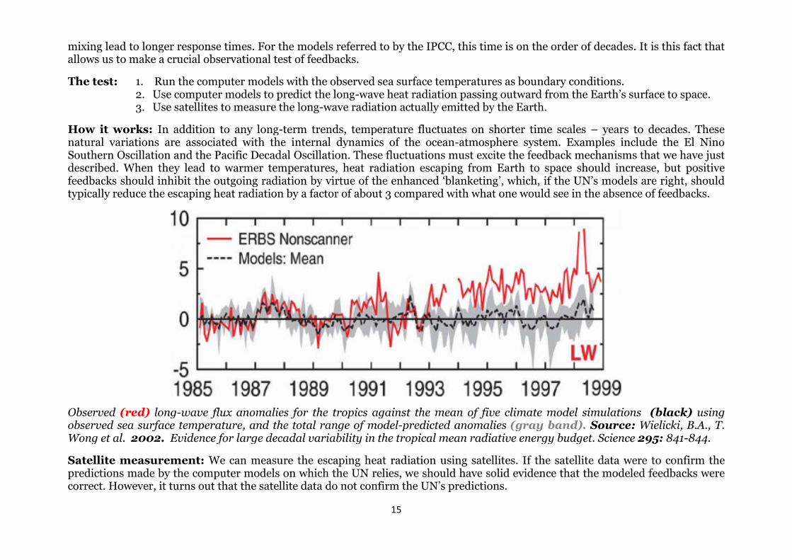
How it works: In addition to any long-term trends, temperature fluctuates on shorter time scales – years to decades. Thesenatural variations are associated with the internal dynamics of the ocean-atmosphere system. Examples include the El NinoSouthern Oscillation and the Pacific Decadal Oscillation. These fluctuations must excite the feedback mechanisms that we have justdescribed. When they lead to warmer temperatures, heat radiation escaping from Earth to space should increase, but positivefeedbacks should inhibit the outgoing radiation by virtue of the enhanced ‘blanketing’, which, if the UN’s models are right, shouldtypically reduce the escaping heat radiation by a factor of about 3 compared with what one would see in the absence of feedbacks.

Observed (red) long-wave flux anomalies for the tropics against the mean of five climate model simulations (black) usingobserved sea surface temperature, and the total range of model-predicted anomalies (gray band). Source: Wielicki, B.A., T.Wong et al. 2002. Evidence for large decadal variability in the tropical mean radiative energy budget. Science 295: 841-844.

Satellite measurement: We can measure the escaping heat radiation using satellites. If the satellite data were to confirm thepredictions made by the computer models on which the UN relies, we should have solid evidence that the modeled feedbacks werecorrect. However, it turns out that the satellite data do not confirm the UN’s predictions.

16

From 1985-89 the models and observations have been tuned to coincide on the graph. However, with the warming after 1989, theobserved outgoing long-wave radiation exceeds 7 times what the models predict. If the observations were only 2-3 times what themodels predict, the result would correspond to no feedback. What we see is much more than this – implying strong negativefeedback. Variability in both the observations and the models (forced by observed sea surface temperature) follows variability intemperature at the Earth’s surface.

Confirmation: These results were sufficiently surprising that they were confirmed by at least four other groups:

CHEN, J., B.E. Carlson, and A.D. Del Genio. 2002. Evidence for strengthening of the tropical general circulation inthe 1990s. Science 295: 838-841.

CESS, R.D., and P.M. Udelhofen. 2003. Climate change during 1985–1999: Cloud interactions determined fromsatellite measurements. Geophys. Res. Ltrs. 30:1: 1019, doi:10.1029/2002GL016128.

HATZIDIMITRIOU, D., I. Vardavas, K. G. Pavlakis, N. Hatzianastassiou, C. Matsoukas, and E. Drakakis. 2004.On the decadal increase in the tropical mean outgoing longwave radiation for the period 1984–2000. Atmos. Chem.Phys. 4: 1419–1425.

CLEMENT, A.C., and B. Soden. 2005. The sensitivity of the tropical-mean radiation budget. J. Clim. 18: 3189-3203.

The above authors did not dwell on the profound implications of these results – they had not intended a test of model feedbacks.They mostly emphasized that the differences had to arise from cloud behavior, a well-acknowledged weakness of current models.However, Chou and Lindzen (2005. Comments on “Examination of the Decadal Tropical Mean ERBS Nonscanner Radiation Datafor the Iris Hypothesis”, J. Climate 18: 2123-2127), say the results imply a strong negative feedback regardless of its cause.

The bottom line is that the Earth’s climate (in contrast to the climate in current climate GCMs) is dominated by a strong netnegative feedback. Climate sensitivity is on the order of 0.3°C, and such warming as may arise from increasing greenhouse gaseswill be indistinguishable from the fluctuations in climate that occur naturally from processes internal to the climate system itself.

Alarming climate predictions depend critically on the fact that models have large positive feedbacks. The crucial question is whetherstrongly-positive temperature feedbacks exist in the real world. The answer, as the satellites have shown, is unambiguously “No”.

The UN predicts a climate sensitivity at least seven times what the satellites have measured. It also predicts that CO2 willaccumulate in the atmosphere at twice the observed rate. Combine these two, and the UN has overestimated the anthropogenictemperature increase in the 21st century approximately 15-fold, just as we calculated last month. End of climate crisis!

17

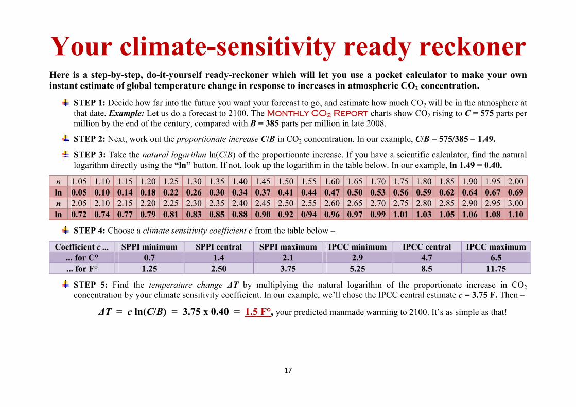
Your climate-sensitivity ready reckonerHere is a step-by-step, do-it-yourself ready-reckoner which will let you use a pocket calculator to make your owninstant estimate of global temperature change in response to increases in atmospheric CO2 concentration.

STEP 1: Decide how far into the future you want your forecast to go, and estimate how much CO2 will be in the atmosphere atthat date. Example: Let us do a forecast to 2100. The Monthly CO2 Report charts show CO2 rising to C = 575 parts permillion by the end of the century, compared with B = 385 parts per million in late 2008.

STEP 2: Next, work out the proportionate increase C/B in CO2 concentration. In our example, C/B = 575/385 = 1.49.

STEP 3: Take the natural logarithm ln(C/B) of the proportionate increase. If you have a scientific calculator, find the naturallogarithm directly using the “ln” button. If not, look up the logarithm in the table below. In our example, ln 1.49 = 0.40.

n 1.05 1.10 1.15 1.20 1.25 1.30 1.35 1.40 1.45 1.50 1.55 1.60 1.65 1.70 1.75 1.80 1.85 1.90 1.95 2.00

ln 0.05 0.10 0.14 0.18 0.22 0.26 0.30 0.34 0.37 0.41 0.44 0.47 0.50 0.53 0.56 0.59 0.62 0.64 0.67 0.69n 2.05 2.10 2.15 2.20 2.25 2.30 2.35 2.40 2.45 2.50 2.55 2.60 2.65 2.70 2.75 2.80 2.85 2.90 2.95 3.00

ln 0.72 0.74 0.77 0.79 0.81 0.83 0.85 0.88 0.90 0.92 0/94 0.96 0.97 0.99 1.01 1.03 1.05 1.06 1.08 1.10

STEP 4: Choose a climate sensitivity coefficient c from the table below –

Coefficient c ... SPPI minimum SPPI central SPPI maximum IPCC minimum IPCC central IPCC maximum

... for C° 0.7 1.4 2.1 2.9 4.7 6.5

... for F° 1.25 2.50 3.75 5.25 8.5 11.75

STEP 5: Find the temperature change ΔT by multiplying the natural logarithm of the proportionate increase in CO2

concentration by your climate sensitivity coefficient. In our example, we’ll chose the IPCC central estimate c = 3.75 F. Then –

ΔT = c ln(C/B) = 3.75 x 0.40 = 1.5 F°, your predicted manmade warming to 2100. It’s as simple as that!

18

The Monthly CO2 Report summarizes key recent scientific papers, selected from those featured weekly at www.co2science.org, that significantlyadd to our understanding of the climate question. This month we review papers about the effects of “global warming” on global climate, ENSOactivity, dengue fever, and grapes and wines. Our final paper gives evidence that the Middle Ages were warmer than today.

Thirty-Second Summary

Climate models lack, or incorrectly parameterize, fundamental processes by which surface temperatures respond to radiativeforcings.

Global warming tends to retard El Niño activity while global cooling tends to promote it. Population dynamics and viral evolution offer the most parsimonious explanation for the observed epidemic cycles of dengue fever,

far more than climatic factors. The expected rise in CO2 concentrations will likely strongly stimulate grapevine production without causing negative repercussions

on quality of grapes and wine. 686 scientists from 401 institutions in 40 countries on the co2science.org Medieval Warm Period database say the Middle Ages

were warmer than today.

Natural and Anthropogenic Influences on Earth's Climate

Lean, J.L. and Rind, D.H, 2008. How natural and anthropogenic influences alter global and regional surface temperatures: 1889 to 2006. Geophysical ResearchLetters 35: 10.1029/2008GL034864.

In an effort "to distinguish between simultaneous natural and anthropogenic impacts on surface temperature, regionally as well as globally,"authors Lean and Rind performed "a robust multivariate analysis using the best available estimates of each together with the observed surfacetemperature record from 1889 to 2006." Results indicated that "contrary to recent assessments based on theoretical models (IPCC, 2007) theanthropogenic warming estimated directly from the historical observations is more pronounced between 45°S and 50°N than at higher latitudes,"which finding, in their words, "is the approximate inverse of the model-simulated anthropogenic plus natural temperature trends ... which haveminimum values in the tropics and increase steadily from 30 to 70°N." Furthermore, as they continue, "the empirically-derived zonal meananthropogenic changes have approximate hemispheric symmetry whereas the mid-to-high latitude modeled changes are larger in the Northernhemisphere." Because of what their analysis revealed, the two researchers concluded that "climate models may therefore lack -- or

SPPI Monthly CO2 Report : : New ScienceBREAKING NEWS IN THE JOURNALS, FROM www.co2science.org

19

incorrectly parameterize -- fundamental processes by which surface temperatures respond to radiative forcings," which is a conclusionwith which all of the world's "climate skeptics" would probably agree, and which should give all of the world's "climate alarmists" pause toconsider the rationality of their calls for dramatic worldwide curtailment of anthropogenic CO2 emissions. To promote such unprecedented andcoercive measures on the basis of model scenarios that "lack -- or incorrectly parameterize -- fundamental processes by which surfacetemperatures respond to radiative forcings" would appear to us to be the height of folly.

ENSO Activity and Climate Change

Langton, S.J., Linsley, B.K., Robinson, R.S., Rosenthal, Y., Oppo, D.W., Eglinton, T.I., Howe, SS., Djajadihardja, Y.S. and Syamsudin, F. 2008. 3500 yr record ofcentennial-scale climate variability from the Western Pacific Warm Pool. Geology 36: 795-798.

The authors used geochemical data obtained from a sediment core extracted from Kau Bay in Halmahera, Indonesia (1°N, 127.5°E) toreconstruct century-scale climate variability within the Western Pacific Warm Pool over the past 3500 years. Among other things learned,Langton et al. report that "basin stagnation, signaling less El Niño-like conditions, occurred during the time frame of the Medieval Warm Period,from ca. 1000 to 750 years BP," which was "followed by an increase in El Niño activity that culminated at the beginning of the Little Ice Age ca.700 years BP." Thereafter, their record suggests that "the remainder of the Little Ice Age was characterized by a steady decrease in El Niñoactivity with warming and freshening of the surface water that continued to the present." In addition, they say that "the chronology of flooddeposits in Laguna Pallcacocha, Ecuador (Moy et al., 2002; Rodbell et al., 1999), attributed to intense El Niño events, shows similar century-scale periods of increased [and decreased] El Niño frequency." As a result, the nine researchers conclude that "the finding of similar century-scale variability in climate archives from two El Niño-sensitive regions on opposite sides of the tropical Pacific strongly suggests that they aredominated by the low-frequency variability of ENSO-related changes in the mean state of the surface ocean in [the] equatorial Pacific." And that"century-scale variability," as they describe it, suggests that global warming typically tends to retard El Nino activity, while global coolingtends to promote it, which finding is in direct contradiction to the alarmist claim that global warming will enhance ENSO events.

Dengue Fever in the Modern World

Wilder-Smith, A. and Gubler, D.J. 2008. Geographic expansion of Dengue: The impact of international travel. Medical Clinics of North America 92: 1377-1390.

The authors note that "the past two decades saw an unprecedented geographic expansion of dengue," reporting that "each year an estimated 50 to100 million dengue infections occur, with several hundred thousand cases of dengue hemorrhagic fever and about twenty thousand deaths." In aneffort to find an explanation for dengue's recent global expansion, Wilder-Smith and Gubler review what is known about the problem, reportingthat "climate has rarely been the principal determinant of [dengue's] prevalence or range," and that "human activities and their impact on localecology have generally been much more significant." In this regard, they cite as contributing factors "urbanization, deforestation, new dams andirrigation systems, poor housing, sewage and waste management systems, and lack of reliable water systems that make it necessary to collect andstore water," further noting that "disruption of vector control programs, be it for reasons of political and social unrest or scientific reservations

20

about the safety of DDT, has contributed to the resurgence of dengue around the world." In addition, they write that "large populations in whichviruses circulate may also allow more co-infection of mosquitoes and humans with more than one serotype of virus," which would appear to beborne out by the fact that "the number of dengue lineages has been increasing roughly in parallel with the size of the human population over thelast two centuries." Most important of all, perhaps, is "the impact of international travel," of which Wilder-Smith and Gubler write that "humans,whether troops, migrant workers, tourists, business travelers, refugees, or others, carry the virus into new geographic areas," which movements,in their words, "can lead to epidemic waves." In conclusion, the authors state that "population dynamics and viral evolution offer the mostparsimonious explanation for the observed epidemic cycles of the disease, far more than climatic factors."

Grape and Wine Responses to Atmospheric CO2 Enrichment

Bindi, M., Fibbi, L. and Miglietta, F. 2001. Free Air CO2 Enrichment (FACE) of grapevine (Vitis vinifera L.): Growth and quality of grape and wine in response toelevated CO2 concentrations. European Journal of Agronomy 14: 145-155.

Working near Rapolano, Siena (Italy), the authors conducted a two-year FACE study of 20-year-old grapevines, where they enriched the airabout the plants to 550 and 700 ppm (compared to ambient CO2 levels in those two years that averaged 363 ppm, as per Mauna Loa data),measuring numerous plant parameters in the process, including - after the fermentation process was completed - "the principal chemicalcompounds that determine the basic red wine quality." Results indicated, in the words of the three researchers, that "elevated atmospheric CO2

levels had a significant effect on biomass components (total and fruit dry weight) with increases that ranged from 40 to 45% in the 550 ppmtreatment and from 45 to 50% in the 700 ppm treatment." In addition, they report that "acid and sugar contents were also stimulated by risingCO2 levels up to a maximum increase in the middle of the ripening season (8-14%)," but they note that as the grapes reached the maturity stage,the CO2 effect on these parameters gradually disappeared. In terms of the primary pigments contained in the wine itself, however, calculationsfrom the bar graphs of their results indicate that in response to the ~50% increase in atmospheric CO2 concentration experienced in going from~363 to ~550 ppm CO2, the concentrations of total polyphenols, total flavoniods, total anthocyanins and non-anthocyanin flavoniods in the winerose by approximately 19%, 33%, 31% and 38%, respectively. Thus, speaking of the future, Bindi et al. conclude that "the expected rise inCO2 concentrations may strongly stimulate grapevine production without causing negative repercussions on quality of grapes andwine." In fact, the ongoing rise in the air's CO2 content might even enhance the quality of the wine.

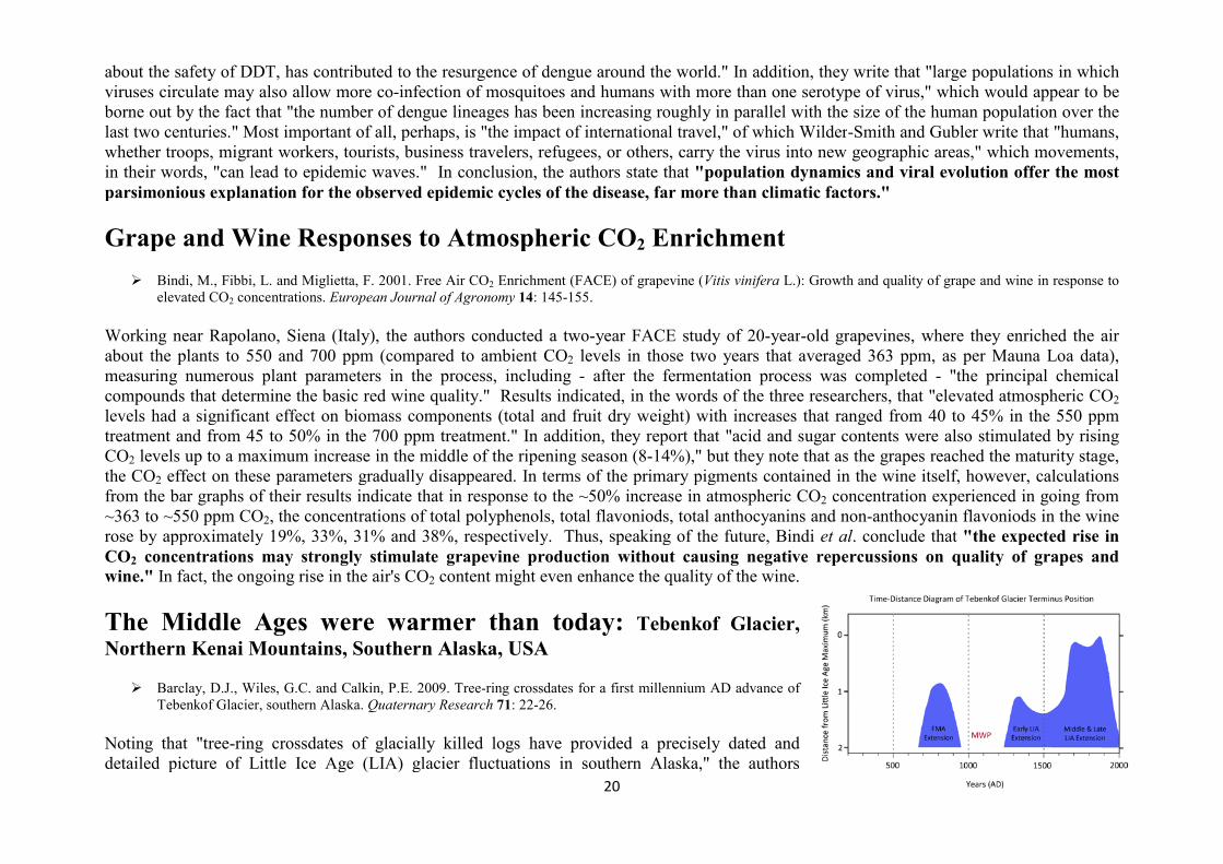
The Middle Ages were warmer than today: Tebenkof Glacier,Northern Kenai Mountains, Southern Alaska, USA

Barclay, D.J., Wiles, G.C. and Calkin, P.E. 2009. Tree-ring crossdates for a first millennium AD advance ofTebenkof Glacier, southern Alaska. Quaternary Research 71: 22-26.

Noting that "tree-ring crossdates of glacially killed logs have provided a precisely dated anddetailed picture of Little Ice Age (LIA) glacier fluctuations in southern Alaska," the authors

21

extended this history back into the First Millennium AD (FMA) by integrating similar data obtained from additional log collections made in1999 with the prior data to produce a "new-and-improved" history of advances and retreats of the Tebenkof Glacier (located in the northernKenai Mountains on the western edge of Prince William Sound) that spans the entire past two millennia. This work revealed that between theFMA and LIA extensions of the Tebenkof Glacier terminus, there was a period between about AD 950 and 1230 when the terminus droppedfurther than two kilometers back from the maximum LIA extension that occurred near the end of the 19th century. It also suggests that thiswarmer/drier period of glacier terminus retreat had to have been much more extreme than what was experienced at any time during the20th century, because at the century's end the glacier's terminus had still not retreated more than two kilometers back from the line of itsmaximum LIA extension.

If you'd like to learn more about climate change science,request a speaker or have any questions,

contact Robert Ferguson, SPPI President.