Contentsuregina.ca/~gingrich/ch64.pdf · Normal Distribution 382 Figure 6.3: The Normal or Bell Curve distribution is at the centre of the distribution. The most common value, the

Contents

6.4 Normal Distribution . . . . . . . . . . . . . . . . . . . . . . . 3816.4.1 Characteristics of the Normal Distribution . . . . . . . 3816.4.2 The Standardized Normal Distribution . . . . . . . . . 3856.4.3 Meaning of Areas under the Normal Curve. . . . . . . 3956.4.4 The General Normal Distribution . . . . . . . . . . . . 3976.4.5 Conclusion . . . . . . . . . . . . . . . . . . . . . . . . 408

380

Normal Distribution 381

6.4 Normal Distribution

The normal probability distribution is the most commonly used probabilitydistribution in statistical work. It is the ‘bell curve’ often used to set testscores, and describe the distribution of variables such as height and weight inhuman populations. The normal distribution also emerges in mathematicalstatistics. For example, probabilities in the binomial probability distributioncan be estimated by using the normal distribution. Also, if random samplesfrom a population are taken, and if the sample sizes are reasonably large,then the means from these samples are normally distributed. It is theselatter uses which are the most important in this textbook, and the normaldistribution is applied to these in the next chapter, and throughout the restof the textbook.

In order to use the normal probability distribution, it is first necessaryto understand a few aspects of its construction, and how to determine prob-abilities using this distribution. These are discussed in this section. A fewcomments concerning the use of the normal distribution are also given. Butwhat is most important to learn at this point is how to determine areasunder the curve of the normal distribution and normal probabilities.

6.4.1 Characteristics of the Normal Distribution

The normal distribution is the bell curve, being bell shaped. However, it isnot just any bell shaped curve, it is a specific probability distribution, withan exact mathematical formula. Sometimes this distribution is referred to asthe Gaussian distribution, named after Gauss, one of the mathematicianswho developed this distribution.

The distribution is shaped as in Figure 6.3, and several characteristicsof the distribution are apparent in this figure. First, note the axes. Thehorizontal axis represents the values of the variable being described. Thevertical axis represents the probability of occurrence of each of the valuesof the variable. Since the curve is highest near the centre, this means thatthe probability of occurrence is greatest near the centre. If a population isnormally distributed, large proportions of the population are near the centre.The farther away from the centre the value of the variable, the lower is theprobability of occurrence of the variable. A population which is normallydistributed has most of its cases near the centre, and relatively few valuesdistant from the centre.

A related characteristic evident from the diagram is that the peak of the


Figure 6.3: The Normal or Bell Curve

distribution is at the centre of the distribution. The most common value,the mode, is at the very centre of the normal distribution. In addition, thedistribution is symmetric around the centre, with one half being a mirrorimage of the other. This means that the median also occurs at the peak ofthe distribution, since one half of the values in the distribution lie on eachside of the peak. Finally, the mean is also at the centre of the distribution,since deviations about the mean on one side have the same probability ofoccurrence of the deviations about the mean on the other side. As a result,the mode, median and mean are equal, and all occur where the distributionreaches its peak value, at the centre of the distribution.

Since the probabilities become smaller, the further from the centre thevariable is, it appears as if the distribution touches the X-axis. In fact, thecurve never quite touches this axis, getting closer and closer, but neverquite touching the X-axis. Such as curve is said to be asymptotic tothe X-axis, approaching but never quite touching the X-axis. For mostpractical purposes, it will be seen that the curve becomes very close tothe X-axis beyond 3 standard deviations from the centre. If a variable isnormally distributed, only a little over 1 case in 1,000 is more than 3 standarddeviations from the centre of the distribution.


Figure 6.4: Normal Distribution of Grades

Example 6.4.1 Normal Distribution of Class Grades

In order to make this discussion more meaningful, suppose an instructorgrades a class on the basis of a normal distribution. In addition, suppose thatthe instructor sets the mean grade at 70 per cent, and the standard deviationof grades at 10 per cent. This is the situation depicted in Figure 6.4, wherethe the mean grade is at the centre of the distribution. In this normal curve,the values along the horizontal axis represent grades of the students, and thevertical axis represents the probability of occurrence of each grade. Recallthat the total area under the whole curve must be equal to 1, since thisarea represents all the cases in the population. The proportion of studentsreceiving each set of grades is then represented by the respective area underthe curve associated with that set of grades.

Figure 6.4 geometrically represents the proportion of students who re-ceive grades between each of the limits 50-60, 60-70, 70-80 and 80-90. Theproportion of students receiving grades between 60 and 70 is given by theproportion of the area under the curve between 60 and 70. Similarly, thearea under the curve between 50 and 60 gives the proportion of studentswho receive between 50 and 60. The proportion who fail, receiving less than


ProportionGrade of Students90+ 0.022880-90 0.135970-80 0.341360-70 0.341350-60 0.1359<50 0.0228

Table 6.21: Normal Grade Distribution, µ = 70, σ = 10

50, is the small area under the curve to the left of 50. The centre of the dis-tribution represents the average grade, and since the curve is highest there,with large areas under the curve, many students receive grades around theaverage. The farther away from the centre, the smaller the area under thecurve, and the fewer the students who receive grades farther from the aver-age. If the instructor does construct grades so that the grades are exactlynormally distributed with µ = 70 and σ = 10, the proportion of studentswith each set of grades is as given in Table 6.21. You can check these figuresonce you have studied the methods later in this section.

There are many normal distributions, and each variable X which is nor-mally distributed, has a mean and standard deviation. If the mean is µ andthe standard deviation is σ, the probability of occurrence of each value ofX can be given as

P (X) =1√2πσ

e−12((X−µ)

σ)2

This expression is not likely to be familiar, and being able to use the normaldistribution does not depend on understanding this formula. However, thisformula shows that there are two parameters for each normal curve, themean µ, and the standard deviation σ. Once these two values have beenspecified, this uniquely defines a normal distribution for X. This meansthat to define a normal distribution, it is necessary to specify a mean andstandard deviation. It also means that anytime a normal distribution isgiven, there will be a particular mean µ, and standard deviation σ associatedwith this distribution.

The formula also means that there are an infinite number of normal dis-


tributions, one for each µ and σ. But each normal curve can be transformedinto the standardized normal distribution. This is the normal distribu-tion which has a mean of µ = 0 and a standard deviation of σ = 1. A simplemathematical transformation can be used to change any normal distributionto the standardized normal distribution. This is given in Section 6.4.4. Theprobabilities for each value of the standardized normal variable are given inAppendix ??. Based on the table in Appendix ??, and the transformationbetween any normal variable X, and the standardized normal variable, Z,the probabilities associated with any normal variable can be determined.

The following section shows how to determine probabilities for the stan-dardized normal distribution, and Section 6.4.4 shows how probabilities canbe obtained for any normal variable.

6.4.2 The Standardized Normal Distribution

The standardized normal distribution is a particular normal distribution, inthat it has a mean of 0 and a standard deviation of 1. In statistical work,the variable which has a standardized normal distribution is termed Z. Instatistics, any time the variable Z is encountered, this denotes a variablewith a mean of 0 and a standard deviation of 1. For Z, the mean is µ = 0and the standard deviation of Z is σ = 1. In Figure 6.5,the distribution ofthe standardized normal variable Z is given. The Z values are given alongthe horizontal axis, and the areas associated with this distribution are givenin Appendix ??.

In each of the figures of the normal distribution, notice that the verticalaxis is labelled the probability, P (Z). The horizontal axis of the standard-ized normal distribution is the value of Z. Since the standard deviation ofZ is σ = 1, these Z values also represent the number of standard deviationsfrom centre. For example, when Z = 2, this represents a point 2 Z valuesabove the mean, but this also represents a value of the variable that is 2standard deviations above the mean of the distribution.

The height of the standardized normal curve at each point indicates theprobability of particular values of Z occurring. These ordinates are not givenin the Appendix ??. Instead, areas under the normal curve are given as theareas in Appendix ??. It will be seen that these are the important values fordetermining the proportions of the population with particular values of thevariable. Also recall that the total area under the curve for any distributionis is 1. Since the normal distribution is symmetrical about the centre of thedistribution, (Z = 0), the area on each side of centre is equal to 0.5. This


Figure 6.5: The Standardized Normal Variable Z

is an important characteristic of the distribution, when determining areasunder the curve. These areas will later be interpreted as probabilities, andalso as proportions of the population taking on specific sets of values of thevariable.

Determining Areas under the Standardized Normal Distribution.In order to use the normal distribution, it is necessary to be able to determineareas under the curve of the normal distribution. These areas are given inAppendix ??. The diagram attached to the table shows a shaded areabetween the centre of the curve and a point to the right of centre. As givenin the diagram, this is the area under the normal distribution between thecentre, Z = 0 and the value of Z indicated. The various possible Z valuesare given in the first column of the table. Note that these are values of Zfrom 0 to 4, at intervals of 0.01.

The second column of Appendix ?? gives the area under the normaldistribution that occurs between Z = 0 and the respective values of Z inthe first colummn. The values in this column represent the shaded area ofthe diagram, that is, the area between the centre and the corresponding Zvalue in the first column. The third column of the table represents the area


under the curve from the value of Z indicated, to +∞, that is, the areaunder the curve beyond the appropriate Z.

Also note that for each Z in the table, the sum of the second and thethird column is always 0.5000. This is because one half, or 0.5000, of thearea is to the right of centre, with the other half to the left of centre. Thehalf of the area to the right of centre is equal to the area from the centre toZ, plus the area beyond Z.

Since the normal curve is symmetric, only one half of the normal curveneed be given in Appendix ??. Areas to the left of centre are equal to thecorresponding areas to the right of centre, but with a negative value for Z.For example, the area under the normal distribution between Z = 0 andZ = −1 is the same as the area under the distribution between Z = 0 andZ = 1.

Determining the various areas under the normal distribution will becomeeasier once the following examples are studied.

Example 6.4.2 Areas Associated with a Specific Z

To begin, Appendix ?? can be used to determine the area

1. Between Z = 0 and Z = 1.

2. Between Z = 0 and Z = −1.

3. Above Z = 1.75.

4. Below −2.31.

These are determined as follows.

1. The area between Z = 0 and Z = 1 is given in Figure 6.6. This canbe read directly from Appendix ??, by going down the Z column untilZ = 1 is reached. To the right of this, in column A, the value of 0.3413is given, and this is the area under the normal distribution betweenZ = 0 and Z = 1. Also note the area of 0.1587 in column B. This isthe area that lies to the right of Z = 1. That is, 0.3413 of the areaunder the normal distribution is between the centre and Z = 1, and0.1587 of the area under the normal distribution lies to the right ofZ = 1. In Figure 6.6, also note that one half of the total area lies tothe left of centre.


Figure 6.6: Areas Associated with Z = 1

2. Since Appendix ?? gives only the area to the right of centre, the onlyway of determining this area is to recognize that by symmetry, the areabetween Z = 0 and Z = −1 is the same as the area between Z = 0and Z = 1. Since the latter area has already been determined to be0.3413, the area under the normal distribution between the centre andZ = −1 is 0.3413.

3. Areas above particular values of Z are given in column B of Ap-pendix ??. The area above Z = 1.75 can be read directly from Ap-pendix ??, by looking at the value of Z = 1.75. In column B, theassociated area is 0.0401. This means that a proportion 0.0401 of thearea, or 0.0401% = 4.01% of the area lies to the right of Z = 1.75.

4. The area below Z = −2.31 is not given directly in the table. Butagain, by symmetry, this is the same as the area above Z = 2.31.Looking up the latter value inAppendix ??, the area associated withthis is 0.0104. This is also the area below Z = −2.31. Also note thatthe area in column B is 0.4896. This is the area between the centreand Z = 2.31, and by symmetry, this is also the area under the normaldistribution that lies between the centre and Z = −2.31.


Example 6.4.3 Areas Between Non Central Z Values

Determine the areas under the normal curve between the following Zvalues.

1. Between -2.31 and +1.75.

2. Between 0.50 and 2.65.

3. Between -1.89 and -0.13.

These areas cannot be determined directly from Appendix ?? withoutsome calculation. The method of obtaining these areas is as follows.

1. Figure 6.7 may be helpful in determining this probability. The areabetween -2.31 and +1.75 can be broken into two parts, the area be-tween -2.31 and 0, and the area between 0 and 1.75. This is necessarybecause Appendix ?? only gives areas between the centre and specificZ values. Once this area has been broken into two parts, it becomesrelatively easy to compute this area. From Figure 6.7, the area be-tween Z = 0 and Z = −2.31 is 0.4896. As shown in Example 6.4.2,this area is the same as the area between Z = 0 and Z = 2.31. Bysymmetry, and from Appendix ??, this area is 0.4896. The area be-tween 0 and 1.75 can be determined from Appendix ?? by looking atcolumn A for Z = 1.75. This area is 0.4599.

The total area requested is thus 0.4896 + 0.4599 = 0.9495. Almost95% of the area under the normal distribution is between Z = −2.31and Z = +1.75.

2. The area between Z = 0.5 and Z = 2.65 is given in Figure 6.8. Againthis area must be calculated. The area requested can be obtained byrecognizing that it equals the area between the centre and Z = 2.65,minus the area between the centre and Z = 0.5. The whole areabetween the centre and Z = 2.65 is 0.4960, obtained in column A ofAppendix ??. This is more than the area requested, and from this,the area between the centre and Z = 0.5 must be subtracted. FromAppendix ??, the latter area is 0.1915.

The area requested is thus 0.4960−0.1915 = 0.3045. This is the shadedarea in Figure 6.8.


Figure 6.7: Area between -2.31 and +1.75

Figure 6.8: Area between 0.5 and 2.65


3. The area between Z = −1.89 and Z = −0.13 must again be calculatedin a manner similar to that used in the last part. The area betweenZ = −1.89 and the centre can be determined by noting that this is thesame as the area between the centre and Z = 1.89. This area is 0.4706.From this, the area between the centre and -0.13 must be subtracted.The latter is the same as the area between Z = 0 and Z = 0.13, andfor the latter Z, the area given in column A of Appendix ?? is 0.0517.

The required area is the area between the centre and -1.89 minus thearea between the centre and -0.13. This is 0.4706 − 0.0517 = 0.4189.This is the requested area.

Example 6.4.4 Obtaining Z values from Specified Areas

Areas are frequently given first, and from this the values of Z are tobe determined. The areas given in columns A and B of Appendix ?? formthe basis for this. However, it may not be possible to find an area in thesecolumns which exactly matches the area requested. In most cases, the areaclosest to that requested is used, and the Z value corresponding to this isused. Find the Z values associated with each of the following.

1. The Z so that only 0.2500 of the area is above this.

2. The 30th percentile.

3. The middle 0.95 of the normal distribution.

4. The Z values for the middle 90% of the distribution, so that the bottomand top 5% of the distribution are excluded.

These all require examination of columns A and B first, and then deter-mination of the Z values associated with the appropriate area. These aredetermined as follows. Figure 6.9 is used to illustrate the first two questions.

1. The Z so that only 0.25 of the area is above this, must lie somewhatto the right of centre, since over one half of the area is to the right ofcentre. Column B of Appendix ?? gives areas above different valuesof Z, and the value closest to 0.25 in this column is the appropriateZ. The two areas closest to 0.25 are 0.2514, associated with Z = 0.67and 0.2483, associated with Z = 0.68. The former of these is closer to0.25 than the latter, so to two decimal places, the Z which is closestis Z = 0.67. Since 0.25 is approximately half way between these two


Figure 6.9: Z for 75th and 30th Percentiles

areas in the table, Z = 0.675 might be reported as the appropriate Z.Note that Z = 0.67 is the 75th percentile, since a proportion of only0.25, or 25% the area is above this Z. This means that 75% of thearea under the curve is below this. Thus in the standardized normaldistribution, P75 = 0.67.

2. The 30th percentile is the value of Z such that only 0.3000 of the areais less than this Z and the other 70% or 0.7000 of the distribution isabove this. This means that the Z so that only 0.3000 of the areais beyond this, must be found. This is obtained by looking downcolumn B until a value close to 0.3000 is found. The closest Z isZ = 0.52, where the area beyond this is 0.3015. The next closest valueis Z = 0.53 associated with an area of 0.2981 beyond this. The formeris a little closer so it will be used. Since we are looking for a Z to theleft of centre, the appropriate Z is −0.52. That is P30 = −0.52 in thestandardized normal distribution. Only 30 per cent of the area underthe curve is below Z = −0.52.

3. The middle 0.95 of the distribution is the area around the centre thataccounts for 0.95 of the total area. This are cannot be directly deter-


Figure 6.10: Middle 0.95 of the Standardized Normal Variable Z

mined, and the method of determing this is illustrated in Figure 6.10.Since the distribution and area requested are both symmetrical, thetotal area of 0.95 in the middle of the distribution can be divided intotwo halves of 0.475 on each side of centre. That is, this amounts to anarea of 0.95/2 = 0.475 on each side of centre. Looking down columnA of Appendix ?? shows that an area of 0.475 between the centre andZ gives a Z of exactly 1.96. That is, Z = 1.96 is associated with anarea of 0.4750 between the centre and this Z. Since the situation issymmetrical around the centre, the appropriate Z on the left is −1.96.That is, going out from centre a Z of 1.96 on either side of centre givesan area of 0.475 on each side of centre, or a total of 0.95 in the middle.The interval requested is from Z = −1.96 to Z = +1.96.

Also note what is left in the tails of the distribution. Below Z = −1.96is an area of 0.025, and above Z = 1.96 is an area of 0.025. That is,there is only 2.5% of the distribution beyond each of these individualZ values. This is a total of 0.05, or 5% per cent, of the distributionoutside these limits. This property will be used extensively in Chap-ter 7. There the interval estimates are often 95% interval estimates,


Figure 6.11: Middle 90% of the Standardized Normal Distribution

requesting the middle 95% of the distribution, leaving out only theextreme 5% of the distribution.

4. This part is a variant of the last part, except looking for the middle90%, rather than the middle 95% of the distribution. The method ofobtaining this is given in Figure 6.11. In this case, the middle 90middle0.9000 of the area is composed of 0.4500 on each side of centre. Thisleaves a total of 0.10 in the two tails of the distribution, or an areaof 0.05 in each tail of the distribution. Looking down column B ofAppendix ?? shows that Z = 1.64 has an area of 0.0505 associatedwith it. The next Z of 1.65 has an area of 0.0495 associated with it.An area of 0.0500 is exactly mdiway between these two values. As aresult, the Z value of 1.645 is used in this case. Above Z = 1.645, thereis exactly 0.05 of the area. By symmetry, there is also an area of 0.05below Z = −1.645. The required interval is from -1.645 to +1.645.This interval contains the middle 90% of the cases in the standardizednormal distribution.

Again, this interval is widely used in the following chapters. In Chapter7, the 90% interval is used, and if the distribution is normal, this is


associated with Z = ±1.645. Later, when conducting hypothesis tests,one of the extremes of 0.05 of the distribution is often excluded, andagain this is associated with a Z of 1.645 from the centre.

6.4.3 Meaning of Areas under the Normal Curve.

The areas under the normal curve have so far been interpreted as nothingmore than areas. Depending on how the normal distribution is used, thereare several possible interpretations of these areas. They may be simplyareas, or they may be interpreted as proportions, percentages, probabilities,or even numbers people. A short discussion of these interpretations follows.

Areas. This requires little further discussion because this is how the nor-mal curve has been interpreted so far. The total area under the whole curveis 1, and each pair of Z values defines an area under the curve. These aresimply areas under the curve, or fractions of the total area under the curve.

Proportions. If a population has a standardized normal distribution, theareas under the curve also correspond to proportions. That is, each pair ofZ values defines a range of values of the variable. The area under the curvebetween these two Z values is the proportion of the population which takeson values within this range. In Example 6.4.3 suppose that the distributionrepresents the distribution of a variable in a population. The total area of 1under the whole curve is equivalent to accounting for the whole population.That is, the sum of all the proportions in a proportional distribution is 1.The proportion of the population between the limits of Z = 0.5 and Z = 2.65is equal to the area within these limits, and this was shown to be 0.3045.Thus 0.3045 of the population is between Z = 0.5 and Z = 2.65.

Percentages. If the proportions are multiplied by 100%, the proportionsbecome percentages. Similarly, the areas multiplied by 100% become per-centages of the population within the respective limits. As in the last para-graph, the percentage of the population between Z = 0.5 and Z = 2.65is 30.45%, if the population has a standardized normal distribution. Alsonote that in Example 6.4.4 the middle 95% of the area was associated withthe range from Z = −1.96 to Z = 1.96. The middle 95% of cases in astandardized normal population is within these limits.


Probabilities. The areas or proportions can also be interpreted as prob-abilities. If a case is randomly selected from a standardized normal popula-tion, then the probability of its being between two specific Z values is thesame as the area between these Z values. Example 6.4.4 shows that 90% ofthe area under the normal curve is between Z = −1.645 and Z = +1.645.As a probability, this could be interpreted as saying that the probabilitythat Z is between −1.645 and +1.645 is 0.90. In symbols, this can be statedas

P (−1.645 < Z < +1.645) = 0.90.

This also means that the probability is 0.05 that Z is either less than −1.645or greater than +1.645. That is,

P (Z < −1.645) = 0.05 and P (Z > +1.645) = 0.05.

Number of Cases. If the proportion or area is multiplied by the numberof cases in the sample or population, this results in the number of cases thatlie within specific limits. For example, suppose that a population has 500people in it. The middle 0.90 of the area has limits for Z of -1.645 and+1.645. This means that 0.90× 500 = 450 people in this population have Zvalues between these Z = −1.645 and Z = +1.645.

Meaning of Z. The values of Z can be interpreted as merely being valuesof Z, distances along the horizontal axis in the diagram of the standardizednormal probability distribution. Remember though that the standardizednormal has a mean of µ = 0 and a standard deviation of σ = 1. Thuseach Z value not only represents a distance from the centre, but it alsorepresents the number of standard deviations from centre. For example,since the standardized normal distribution has a standard deviation of 1,if Z = 1, then this Z is one standard deviation above the mean. Z = 2represents a point which is two standard deviations above the mean. Thepoint on the horizontal axis where Z = −1.6 is 1.6 standard deviations tothe left of centre, or below the mean.

Some of the rules concerning the interpretation of the standard deviationgiven on page 254 of Part I of this text can be illustrated using this inter-pretation of the Z value. In Example 6.4.2 above, the area between Z = 0and Z = 1 was shown to be 0.3413, with the area to the right of Z = 1being 0.1587. If a population has a standardized normal distribution, thena proportion 0.3413 of the population is between the mean and 1 standard


deviation above centre. This is 0.3413 × 100% = 34.13%, or rounded off,34% of the total cases. On the basis of the symmetry of the curve, another0.3413, or 34% are between the centre and 1 standard deviation below cen-tre. In total, there are thus 0.3413 + 0.3413 = 0.6826 or 68.26% of the totalcases within one standard deviation of the mean. Rounded off, this is 68% ofthe cases, or just over two thirds of the cases within one standard deviationof the mean.

The proportion of 0.1587 being to the right of Z = 1 means that only0.1587, or 16% of the cases in the standardized normal lie more than 1standard deviation above the mean. Similarly, another 16% of the cases aremore than one standard deviation below the mean. Together this meansthat about 32% of the population is farther than one standard deviationaway from the mean.

Example 6.4.4 and Table 6.10 showed that the middle 95% of the normaldistribution was between Z = −1.96 and Z = 1.96. That is, within 1.96standard deviations on either side of the mean, there are 95% of all the casesin the standardized normal distribution. While this is an exact determina-tion, this produces the rough rule of page 254 of Part I of this text that 95%of all cases are within two standard deviations of the mean. Also note thatthis implies that approximately 5% of of the cases are farther than two Zvalues, or two standard deviations away from the mean.

Finally, you can use the normal probabilities in Appendix ?? to showthat within three standard deviations of the mean, the standardized normalhas 99.74% of all the cases. Only 0.26% of all the cases are farther thanthree standard deviations from the mean in the case of the standardizednormal.

6.4.4 The General Normal Distribution

The standardized normal distribution is a special case of the normal distribu-tion. In general, a normal variable X has mean µ and standard deviation σ.This section shows how this general normal distribution can be transformedinto the standardized normal distribution, and how the transformation cango the other way as well. This means that Appendix ?? can always be usedto determine areas or probabilities associated with the standardized normaldistribution, and the transformation used to associate these with any otherdistribution.


Figure 6.12: The General Normal Variable X with Mean µ and StandardDeviation σ

Notation. In order to keep track of each normal curve, it is useful tohave a general notation. Suppose the variable X is a normally distributedvariable, with a mean of µ and a standard deviation of σ. Let this be denotedby Nor(µ, σ). That is, . That is,

X is Nor(µ, σ)

is a short form for saying that variable X is normally distributed with meanµ and standard deviation σ. Given this notation, the standardized normalvariable Z with mean 0 and standard deviation 1 can be denoted by

Z is Nor(0, 1).

The general normal distribution is pictured in Figure 6.12. The variableX is normally distributed with the mean µ at the centre of the distribution.The standard deviation is σ. This is a little more difficult to show in thediagram, but it can be seen what the approximate distance from the centreto one standard deviation on each side of the mean is.


In order to transform this variable X into the standardized normal dis-tribution, the following transformation is used.

Z =X − µ

σ

That is, if the mean µ is subtracted from X, and this difference is dividedby σ, the result is to produce a new variable Z. This Z is the same Z asencountered earlier, that is, it has mean 0 and standard deviation 1.

This particular transformation of Z is referred to as standardization,and is widely used in statistical work. Standardization refers to the processof taking a variable with any mean µ and any standard deviation σ andproducing a variable with a mean of 0 and a standard deviation of 1. Thevariable with the mean of 0 and standard deviation of 1 is referred to asa standardized variable. If the distribution of X is normal, then thecorresponding standardized variable is given the symbol Z, and this is thestandardized normal variable of the last section.

It should be possible to see that

X − µ

σ

has a mean of 0. Note that the mean of X is µ, so that when µ is subtractedfrom each value of X, the mean of these differences will be 0, with thenegative and positive deviations cancelling. This is essentially the same asthe property that ∑

(Xi − X̄) = 0

as shown in Chapter 5, except that X̄ is replaced by the true mean µ. Theproof that the standard deviation of the above expression is 1 requires alittle more algebra than has been introduced in this textbook. However,this property can be recognized in an intuitive manner by noting that eachdifference X −µ is divided by the standard deviation σ. Since the standarddeviation of X is σ, this is like dividing σ by σ, producing a value of 1.

The transformation can be used to go in the other direction as well.Solving the first transformation for X gives the following:

Z =X − µ

σ

Zσ =X − µ

σσ


X = µ + Zσ

X = µ + Zσ

The latter expression is the important one. In that expression, if Z isgiven, and if µ and σ are known, then the value of X can be calculated.This expression will be used when areas or probabilities under the normaldistribution are given first, and the values of X that corresponds to theseare required. From the original areas which are specified, the Z value canbe obtained. Then the values of X can be determined by using

X = µ + Zσ

The use of these transformations should become clearer in the followingexamples.

Example 6.4.5 Distribution of Socioeconomic Status

The Regina Labour Force Survey asked respondents their occupation.The Blishen scale of socioeconomic status was used to determine the socioe-conomic status of each occupation. The Blishen scale is an interval levelscale with a range of approximately 100. It is based on a combination ofthe education level and income of the occupation of the respondent. A lownumber on the scale indicates low socioeconomic status, and a high valueindicates an occupation with high status or prestige. The mean socioe-conomic status of those surveyed was 48 and the standard deviation was14. Assuming that socioeconomic status is a normally distributed variable,determine

1. The proportion of the population with socioeconomic status of 65 ormore.

2. The percentage of the population with socioeconomic status of lessthan 40.

3. The proportion of the population with socioeconomic status between40 and 65.

4. The socioeconomic status so that only 10% of the population hasgreater socioeconomic status.

5. The 35th percentile of socioeconomic status.


Let X represent the distribution of socioeconomic status (SES). Thedistribution of X is normal with µ = 48 and σ = 14, that is,

X is Nor(48, 14).

Figure 6.13 illustrates this distribution diagramatically, with SES along thehorizontal axis, and the mean at 48. The first three parts of this questionuse this figure. In obtaining the required proportions and percentages, it isuseful to place both the X and Z values on the same horizontal axis. Thenormal curve is the same in both situations, all that the transformation fromX to Z really does is change the units on the horizontal axis. When thehorizontal axis is X, the units are units of socioeconomic status, with themean status being at X = 48. Transforming the X into Z transforms thehorizontal axis into Z values. Since the standard deviation of Z is 1, these Zvalues are also represent the number of standard deviations for centre. Thefollowing description shows how the transformation can be used to determinethe required probabilities.

1. The proportion of the population with SES of 65 or more is representedby the area under the normal curve in Figure 6.13 that lies to the rightof an SES of 65. This area can be determined by calculating the Zassociated with X = 65, and then using the normal table. Since

Z =X − µ

σ

for X = 65,

Z =65− 48

14=

1714

= 1.21

to two decimal places. In Appendix ??, when Z = 1.21, the area incolumn B is 0.1131. This is the area under the normal distributionthat lies to the right of Z = 1.21 or to the right of X = 65. Thus theproportion of the population with SES of 65 or more is 0.1131.

Note that SES of 65 is associated with Z = 1.21. This is equivalentto saying that SES of 65 is 1.21 standard deviations above average.There is thus a proportion 0.1131 of the population with SES of 1.21standard deviations or more above the mean.

2. The percentage of the population with SES of less than 40 is associatedwith an X to the left of centre, as indicated in Figure 6.13. For X = 40,


Figure 6.13: Distribution of SES

the Z value is

Z =X − µ

σ=

40− 4814

=−814

= −0.57

Note that Z is negative here, since this value is to the left of centre.Since the curve is symmetrical, the required area under the curve tothe left of Z = −0.57 is the same as the area under the curve to theright ot Z = +0.57. From column B of Appendix ?? this area is0.2843. The percentage of the population with SES of less than 40 isthus 0.2843 × 100% = 28.43%, or rounded to the nearest tenth of apercentage point, this is 28.4% of the population.

3. The proportion of the population between SES of 40 and 65 can bequickly determined on the basis of the Z values already calculated.The required proportion is the area under the normal curve betweenX = 40 and X = 65. This is equal to the area between X = 40 and thecentre plus the area between the centre of the distribution and X = 65.Since X = 40 is associated with Z = −0.57, column A of Appendix ??shows that the area between this value and centre is 0.2157. The areabetween centre and X = 65 or Z = 1.21 is 0.3869. The required area is


Figure 6.14: 90th Percentile of SES

thus 0.2157 + 0.3869 = 0.6026. Just over six tenths of the populationhave SES between 40 and 65.

4. The SES so that only 10% of the population have greater status isgiven on the right side of Figure 6.14. If only 10% of the populationhave greater status, then this is equivalent to the upper 10% of thedistribution, or the upper 0.10 of the area under the normal curve.What is given here is the area under the curve, and from this, theX value of SES must be determined. The first step in doing this isto recognize that when an area is given, the Z value associated withthis area can be determined. Since the area given is in the tail of thedistribution, column B of Appendix ?? is used to find this area. TheZ value which comes closest to producing an area of 0.1000 in columnB is Z = 1.28. This is considerably closer to the required area thanthe next Z of 1.29. This means that only 10% of the population havestatus more than 1.28 standard deviations above the mean.

The next step is to determine the exact SES associated with this. Thisis done by using the reverse transformation, going from Z to X. It


was shown thatX = µ + Zσ

and since the mean is µ = 48 and the standard deviation is σ = 14,

X = µ + Zσ = 48 + (1.28× 14) = 48 + 17.92 = 65.92

Rounding this off to the nearest integer, the SES so that only 10 percent of the population has greater status is 66. Note that this is the90th percentile of SES. That is, P90 is the value of SES so that 90%of the population has lower status, and only 10% have greater status.Thus P90 = 66 in this distribution.

5. Similar considerations are used to obtain the 35th percentile. This isthe value of SES so that 35%, or 0.3500 of the distribution is less thanthis. Looking down column B in Appendix ??, the Z which comesclosest to producing an area of 0.3500 in the tail of the distributionis Z = 0.39, although Z = 0.38 is almost as close. Since this is tothe left of centre, the appropriate Z is Z = −0.39. Using the reversetransformation to find the value of X gives

X = µ + Zσ = 48 + (−0.39× 14) = 48− 5.46 = 42.54

Note the importance of remembering Z is negative in this case, becausethe required SES is below the mean. The 35th percentile of SES is42.5, or 43. That is P35 = 43.

Example 6.4.6 Graduate Record Examination Test Scores

The verbal test scores for U.S. college seniors taking the Graduate RecordExaminations (GRE) in Clinical Psychology and Computer Science over theyears 1984-1987 are contained in Table 6.22.

1. For each of the two groups, assume the distribution of test scores isnormal. Use the mean and standard deviation listed to work out thepercentage of students who would be expected to have test scores ineach interval, based on the normal curve.

2. Compare the percentages you have with the percentages from the re-spective frequency distributions in Table 6.22. Explain whether theactual test scores appear to be normally distributed or not.


Distribution of Test Scores(Per Cent by Discipline)

Clinical ComputerTest Score Psychology Science

300 or less 1.5 8.2300-400 12.9 20.0400-500 34.2 25.9500-600 32.9 24.6600-700 15.1 15.0

700 and over 3.4 6.3

Number of Students 15,169 16,593Mean Test Score 502 482

Standard Deviation 102 133

Table 6.22: GRE Test Scores

3. Assuming the test scores are normally distributed, what test scoreshould a student taking the Clinical Psychology test obtain in orderto assure that he or she is in the 85th percentile?

Answer.

1. For Clinical Psychology, the normal distribution has µ = 502 andσ = 102, and for Computer Science, µ = 482 and σ = 133. For eachof the values 300, 400, etc., Z values must be calculated in order todetermine the appropriate areas and percentages. For example, forClinical Psychology, the Z value for X = 300 is

Z =X − µ

σ=

300− 502102

= −1.98.

and for X = 400 is

Z =X − µ

σ=

400− 502102

= −1.00.

Using this same method, Table 6.23 gives the values of Z for eachof the X values in Table 6.22. In addition, based on column A of


Appendix ??, this table gives the areas between each Z and the meanof the normal distribution.

Psychology Computer ScienceX Z Area Z Area

300 -1.98 0.4761 -1.37 0.4147400 -1.00 0.3413 -0.62 0.2324500 -0.02 0.0080 0.14 0.0557600 0.96 0.3315 0.89 0.3133700 1.94 0.4738 1.64 0.4495

Table 6.23: Z Values and Areas for GRE Test Scores

For Clinical Psychology, the area below X = 300 is the area belowZ = −1.98, and from column B of Appendix ??, this is 0.0239. Thearea between X = 300 and X = 400 is the area between Z = −1.98and Z = −1.00. From Table 6.23, this is 0.4761 − 0.3413 = 0.1348.Similarly, the area between X = 500 or Z = −0.02 and X = 400 orZ = −1.00 is 0.3413− 0.0080 = 0.3333.

The area between X = 500 and X = 600 is the same as the areabetween Z = −0.02 and Z = 0.96. These two areas are added toproduce this total area, so this is 0.0080 + 0.3315 = 0.3395. Theseareas must be added together because they are on opposite sides ofthe centre. The area between X = 600 or Z = 0.96 and X = 700 orZ = 1.94 is 0.4738−0.3315 = 0.1423. Finally, the area above X = 700is the area above Z = 1.94. From Appendix ?? this is 0.0262.

For the Computer Science distribution, the method is the same. Thearea below X = 300 is the area below Z = −1.37, and from Ap-pendix ??, this is 0.0853. The area between X = 400 or Z = −0.62 andX = 300 or Z = −1.37 is 0.4147− 0.2324 = 0.1823. The area betweenX = 400 or Z = −0.62 and X = 500 or Z = 0.14 is 0.2324 + 0.0557 =0.2881. The area between X = 500 or Z = 0.14 and X = 600 orZ = 0.89 is 0.3133 − 0.0557 = 0.2576. The area between X = 600 orZ = 0.89 and X = 700 or Z = 1.64 is 0.4495− 0.3133 = 0.1362. Thearea above X = 700 or Z = 1.64 is 0.0505.

All these areas under the normal curve are converted into percentages


and are reported in Table 6.24. There the percentages from the normaldistribution can be compared with the actual percentages.

Distribution of Test Scores(Per Cent by Discipline)

Clinical Psychology Computer ScienceTest Score Actual Normal Actual Normal

300 or less 1.5 2.4 8.2 8.5300-400 12.9 13.5 20.0 18.2400-500 34.2 33.3 25.9 28.8500-600 32.9 34.0 24.6 25.8600-700 15.1 14.2 15.0 13.6

700 and over 3.4 2.6 6.3 5.1

Table 6.24: GRE Test Scores - Actual and Normal

2. Based on the distributions in Table 6.24, it can be seen that both theactual Clinical Psychology and Computer Science test scores are verysimilar to the percentages obtained from the normal distribution. Asa result, it could be claimed that the actual test scores are normallydistributed. Later in the textbook, the chi square test will be used totest the hypothesis that the grades are normally distributed. For now,close inspection of the table shows that the actual test scores are veryclose to normal.

In terms of the differences that do appear, for Clinical Psychology,the actual scores have only 12.9 + 1.5 = 14.4% below 400, while thenormal curve would indicate there should be 2.4 + 13.5 = 15.9%. Thenormal curve has fewer above 600 (16.8%) than the 18.5% who actuallyscored above 600. There are also minor differences in the middle ofthe distribution.

For Computer Science, there are more test scores in the 300-400 range(20.0%) than in this range in the normal curve (18.2%). Also, thereare considerably more test scores above 600 (21.3%) than indicatedby the normal distribution (18.7%). As a result, there are fewer test


scores in the middle range, between 400 and 600, than in the case ofthe normal distribution.

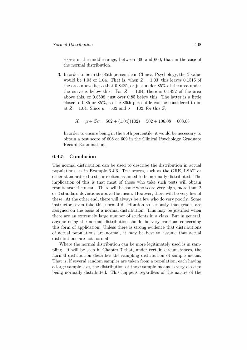
3. In order to be in the 85th percentile in Clinical Psychology, the Z valuewould be 1.03 or 1.04. That is, when Z = 1.03, this leaves 0.1515 ofthe area above it, so that 0.8485, or just under 85% of the area underthe curve is below this. For Z = 1.04, there is 0.1492 of the areaabove this, or 0.8508, just over 0.85 below this. The latter is a littlecloser to 0.85 or 85%, so the 86th percentile can be considered to beat Z = 1.04. Since µ = 502 and σ = 102, for this Z,

X = µ + Zσ = 502 + (1.04)(102) = 502 + 106.08 = 608.08

In order to ensure being in the 85th percentile, it would be necessary toobtain a test score of 608 or 609 in the Clinical Psychology GraduateRecord Examination.

6.4.5 Conclusion

The normal distribution can be used to describe the distribution in actualpopulations, as in Example 6.4.6. Test scores, such as the GRE, LSAT orother standardized tests, are often assumed to be normally distributed. Theimplication of this is that most of those who take such tests will obtainresults near the mean. There will be some who score very high, more than 2or 3 standard deviations above the mean. However, there will be very few ofthese. At the other end, there will always be a few who do very poorly. Someinstructors even take this normal distribution so seriously that grades areassigned on the basis of a normal distribution. This may be justified whenthere are an extremely large number of students in a class. But in general,anyone using the normal distribution should be very cautious concerningthis form of application. Unless there is strong evidence that distributionsof actual populations are normal, it may be best to assume that actualdistributions are not normal.

Where the normal distribution can be more legitimately used is in sam-pling. It will be seen in Chapter 7 that, under certain circumstances, thenormal distribution describes the sampling distribution of sample means.That is, if several random samples are taken from a population, each havinga large sample size, the distribution of these sample means is very close tobeing normally distributed. This happens regardless of the nature of the


population from which the sample is drawn. In the next section, it will beseen that the normal distribution can also be used to provide approximationsof normal probabilities. It is these latter uses which are more legitimate,and in this textbook, these are the main uses for the normal distribution.

Documents

Contentsuregina.ca/~gingrich/ch64.pdf · Normal Distribution 382 Figure 6.3: The Normal or Bell Curve distribution is at the centre of the distribution. The most common value, the