Geppetto – Population Synthesis Software

D e p a r t m e n t o f

B i o i n f o r m a t i c s ,

T e c h n i o n , I s r a e l

I s r a e l I n s t i t u t e o f

T e c h n o l o g y , H a i f a ,

I s r a e l

1 / 1 / 2 0 0 8

Amit Zur, Daniel Anvar

Geppetto is a population synthesis tool. It offers

numerous features such as creating populations from

different ancestral origins, creating admixed

individuals, and finally also a pedigree creation

feature. Compatible with the HapMap genome data

format, as well as capable of handling its own, simpler

format, this tool can prove useful in meeting research

needs that deal with populations, pedigrees and

mapping by admixture linkage disequilibrium (MALD).

Geppetto – Population Synthesis Software

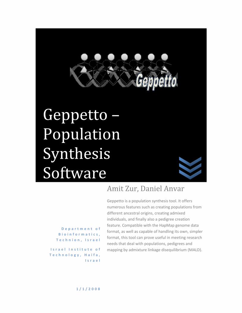
Table of Contents Geppetto Overview ......................................................................................................................... 4

Population Creation..................................................................................................................... 4

Project Aims................................................................................................................................. 4

General Information .................................................................................................................... 4

Authors and Contacts .................................................................................................................. 5

Run the Geppetto program ............................................................................................................. 6

Executing Geppetto ..................................................................................................................... 6

Geppetto Input File Format ......................................................................................................... 6

Input File Parameters List ........................................................................................................ 6

Geppetto Parameters ...................................................................................................................... 8

Common Input Parameters ......................................................................................................... 8

Chromosome Loaders ............................................................................................................... 10

Loading Genotype Data ......................................................................................................... 10

Binary Chromosome Loaders ................................................................................................ 10

Disease Model ........................................................................................................................... 11

Disease Model File Format .................................................................................................... 11

Pedigree File – PedFile............................................................................................................... 12

PedFile Format....................................................................................................................... 12

PedFile Example..................................................................................................................... 13

Recombination Rate Producer .................................................................................................. 14

Genotype Data .............................................................................................................................. 16

HapMap Genotype Data ............................................................................................................ 16

HapMap Genotype File Format ............................................................................................. 17

How to Use HapMap Genotype Files .................................................................................... 18

Geppetto Genotype Data .......................................................................................................... 18

Geppetto Genotype File Format ........................................................................................... 19

How to Use Geppetto Genotype Files ................................................................................... 20

Population Creation Scenarios ...................................................................................................... 21

Create from Pedigree Scenario ..................................................................................................... 22

Input .......................................................................................................................................... 22

Output ....................................................................................................................................... 23

Overview – How it works ........................................................................................................... 23

Plain Scenario ................................................................................................................................ 25

Input .......................................................................................................................................... 25

Output ....................................................................................................................................... 26


Stratification Scenario ................................................................................................................... 28

Input .......................................................................................................................................... 28

Output ....................................................................................................................................... 30


Admixed Populations Scenarios .................................................................................................... 32

Hybrid Isolated Scenario................................................................................................................ 33

Input .......................................................................................................................................... 33

Output ....................................................................................................................................... 35

Overview – How It Works .......................................................................................................... 35

Continuous Gene Flow Scenario.................................................................................................... 37

Input .......................................................................................................................................... 37

Output ....................................................................................................................................... 39


Straight Admixed Scenario ............................................................................................................ 41

Input .......................................................................................................................................... 42

Output ....................................................................................................................................... 43


References ..................................................................................................................................... 45

Geppetto Overview Geppetto is population synthesis software. It can “create” genomes of individuals, according to

genotype data provided by the user – it creates the genomes by assigning an allele to each

marker in the genotype data. The genotype data input defines probabilities for each allele in

each marker, and Geppetto assigns the alleles according to the alleles’ probabilities.

Population Creation There are several methods of population creation. Geppetto supports 6 population creation

scenarios, which are detailed in Population Creation Scenarios section.

In Geppetto, there are essentially 3 ways of creating a population: The first is non-admixed

population creation, where each person genome from the population is created straight from

the genotype data. The second is admixed population creation – each person is a result of

different types of populations (or ancestries) that their mating (or mixing) over time yielded

genomes of mixed ancestries. Geppetto simulates that scenario – it creates the genomes of the

founders (people that their genomes are originated in one population) and actually mates them,

while considering recombination points, to produce mixed genomes. The third population

creation way is done through creating an entire pedigree – given a pedigree, Geppetto creates

all the genomes of the pedigree’s individuals, while taking into account all the relations between

them.

Geppetto also has the ability to create individuals within the created population who posses a

certain trait, or sickness, that is described by the user (a disease model ).

Project Aims Geppetto Aims are to provide an extensible tool, which can create diverse populations in

different scenarios, with sick and healthy individuals to a certain genetic sickness. That can be of

many uses:

Help research of a genetic disease: through inspection of the created individual’s

genomes, one can assess whether a disease is linked to a certain population, or a certain

marker within diverse population, etc.

Test labeling programs (Ancestrymap Software n.d.): simulating the labeling software on

created populations to verify their correctness.

Help to design a genetic panel microarray experiments: By testing the selected genetic

panel (a group of alleles which is supposed to be used in microarray gene hunting) on

synthesized populations first, one can save a lot of time and money, before issuing the

final panel.

General Information Geppetto is written in Java. Due to the size of the genotype data, the size of the output (each

person’s genome is a collection of text files), and different population scenarios, Geppetto uses

large amounts of CPU time and memory, uses the hard drive, and its execution time may vary

between few seconds to several minutes (depending on the type of population creation and the

genotype data). In order to keep track of Geppetto execution, you can see the console logs

throughout the execution (Tip: use the trace verbosity level).

The admixed population creation scenarios, which define sick people to create are most prone

to lengthy execution times – Geppetto tries to create a sick person, and then according to the

disease model, determines if indeed the created person is sick. If the person is not sick,

Geppetto tries again, and that can result in long execution time. Therefore, the execution time is

dependent on the disease model and the complexity of the created population (when admixed

population creation methods are the most complex).

Geppetto is highly configurable – the user can define an extensive disease model, define the

rate of genetic recombination in the pedigree, define number of sick and healthy people to

produce, define the number of generation of admixture that the created population underwent

(see the admixed population creation scenarios for more info: HI, CGF and Straight Admixed),

and more.

Authors and Contacts Geppetto was written by Amit Zur and Daniel Anvar, as an undergraduate project in the

department of bioinformatics, Technion, Israel, under the guidance of Prof. Dan Geiger and

Sivan Bercovici.

Run the Geppetto program The Geppetto program must be executed with an input file. The input file defines all the

parameters for the program execution, and you can find its structure and some examples in this

section.

Executing Geppetto From a console line, run “Java Geppetto <input file path>” with your input file (which complies

with the Geppetto input file format.

Tip: to run Java with more memory, use the flag “-mx1000m” for virtualizing 1000 mega of Java

heap memory.

There are 6 population creation methods (or scenarios): Plain, Stratification, Create from

Pedigree, Hybrid Isolated, Continuous Gene Flow, and Straight Admixed. See explanations about

each population creation scenario in the Population Creation Scenarios section.

Geppetto Input File Format The input file is a simple text file. Each of the parameters is defined with a “#” sign following by

the parameter name, and after a “=” sign the parameter value:

#<parameter name> = <parameter value>

The parameters are case-insensitive.

All the lines in the input file which don’t correspond to a valid parameter name are ignored.

Input File Parameters List

The following table lists all the parameters that can be defined in the Geppetto input file. Some

parameters are common to all population creation scenarios, and are marked as bold (they are

also explained in detail in the Common Geppetto Parameters section).

Name Description

#Creation Method The population creation scenario method

#Genotype Genotype data

#Output Folder Path of the program output folder

#Seed Seed of the program’s random operations

#ChrLoadersBinaries Path of the chromosome binaries folder

#Recombination Rate Recombination Rate function

#Disease Model File Disease Model file path

#pedigree file Pedigree PedFile path

#healthy people Number of healthy people to produce

#sick people Number of sick people to produce

#generations Number of generations of created population admixture

#number of populations Number of populations (ancestries) involved in the

created population

#populations fractions Fractions of the ancestry population in the created

population

#Lambda Lambda parameter (simulates number of generations in

the created admixed populations)

#Trace Trace verbosity flag

#Use Garbage Collection Call Java’s Garbage Collector flag

Geppetto Parameters The Geppetto program operates according to user input parameters, which are defined in the

Geppetto Input File .

There are common input parameters, shared by all the population creation scenarios, and there

are some parameters which are used under different scenarios. You can find extensive

information about input parameters of each scenario under each population creation scenario

section.

Common Input Parameters All population creation scenarios of the Geppetto program share some common input

parameters, some are required and some are optional.

The following table lists the list of common program parameters.

Chromosome

Loaders

The chromosome loaders hold the genotype data which the program will

create the population’s genomes by.

They hold information about the markers that represents the genome. The

program will create, according to the population creation scenario and in a

randomly fashion, populations’ genomes by assigning values to each marker.

See more information about the different types of loaders, how to use them

in the program and more in the Chromosome Loaders section.

Seed (optional) The program’s random operations seed. The program uses random objects

to create the population in a pseudo-randomly fashion. The seed specified is

the source for all the pseudo-random actions that the program takes.

Meaning, every time the program runs with the same seed it produces equal

results.

If this parameter is not set, the seed will be randomly created and will be

reported to the user, so a reproduction is possible.

Set in the input file:

Output folder

(optional)

A path of a folder on the file system, which the output of the program will be

plotted to. See each of the population creation scenarios sections for mode

details on their output.

If this parameter is not set, the default output folder will be “<<folder of the

input file >\Output>”

#Seed = <number of type long>


Trace (Optional) Flag that controls the verbosity level of the program’s output to the console

line. If this flag is set and its value is “True”, then the program’s verbosity is

enhanced.

The default value is False, meaning that the program produces less trace

lines in the console.


Use Garbage

Collection

(Optional)

Flag that controls the Java Garbage Collector calling schedule.

The Java Garbage Collection is fired in order to free up memory for the

program to use. Since the Geppetto program uses large amounts of

memory, when creating big populations or handling big chromosome

loaders, there might be a memory shortage issue.

Use this flag in order to call the garbage collector more often (by setting it to

“true”), and by that freeing up memory as the program progresses, and

enable the program to complete. You must note that the performance of the

program might be reduced.

The default value is False, meaning that the program will not call Java

Garbage Collection intentionally.


#use garbage collection = <true / false>

#trace = <true / false>

#output file= <output folder’s path>

Chromosome Loaders The chromosome loaders are objects that the program uses to hold the genotype data which

the program will create the population’s genomes by, for a given chromosome.

They hold information about the markers that represents the chromosome. The program will

create, according to the population creation scenario and in a randomly fashion, populations’

genomes by assigning values to each marker at each chromosome.

The chromosome loaders obtain their data from genotype data. The genotype data can be given

to Geppetto using the currently supported genotype data format: HapMap genotype data, and

Geppetto genotype data. See those sections for more details.

Loading Genotype Data

You can load genotype data for several chromosomes, by specifying in the input file

#genotype = <path to genotype data file(s)>

See more information in the Genotype Data section.

Binary Chromosome Loaders

The genotype data files are parsed by the Geppetto program into the chromosome loaders

objects, which are the data structure the program uses. Parsing of the genotype text files is a

long and memory consuming operation. Therefore, the Geppetto program, after parsing the text

files, saves the created chromosome loaders as binary files. The chromosome loaders binary

files are saved under the <output folder>\ChrLoaders folder.

You can use those binary chromosome loaders as input to the Geppetto program. Using them

will speed up the program execution (parsing of the text files are not necessary), and it is

recommended.

How to Use Binary Chromosome Loaders

In order to run Geppetto with binary chromosome loaders files, specify in the input file the

following: Just specify a path to the folder that holds those binaries. Each file in that folder (that

was created in a previous run of the program) has a filename of “ChrLoader??.bin” name.

Specify the binaries folder in the following way in the input file:

#ChrLoadersBinaries = <ChrLoaders folder path>

Example:

Say we already ran the program with text genotype data, and the output folder was set as

“c:\output”. Then from that run, a folder “c:\output\ChrLoaders” was created. In the next

execution of Geppetto, we can define the following line:

#ChrLoadersBinaries = D:\output\ChrLoaders

Disease Model The Disease Model entity defines the model, on top of which a person from a created

population will be marked as “sick” (or will posses a certain trait. For the simplicity of the

discussion, we will refer to “sickness”). In Geppetto, a person will be created, and then, if he is

supposed to be sick, his genome will be checked against the disease model, to determine his

sickness status.

The Geppetto Disease Model enables defining genetic diseases – diseases that are characterized

by a specific allele of a specific marker, or combination of such markers. This in fact, lets you

define disease that it is linked to certain markers in the genome.

For example, say we have a disease that is linked to a certain VNTR (marker) allele, in 95% of the

cases. Then you can define the Disease Model to reflect that: specify the RS number of the

marker (or VNTR), its “infected” allele, and 0.95 as the probability of a person that possesses

this marker to be sick with that disease.

The Geppetto Disease Model also lets you define several combinations of markers and alleles

that are linked to the disease, with different probabilities. For example, you can define that the

disease is linked to 2 joined markers with the probability of 0.3, and to another 3 markers with

probability of 0.9. When creating the population you can check amongst the sick people, which

of the markers sequence are more linked to the disease, in the created population.

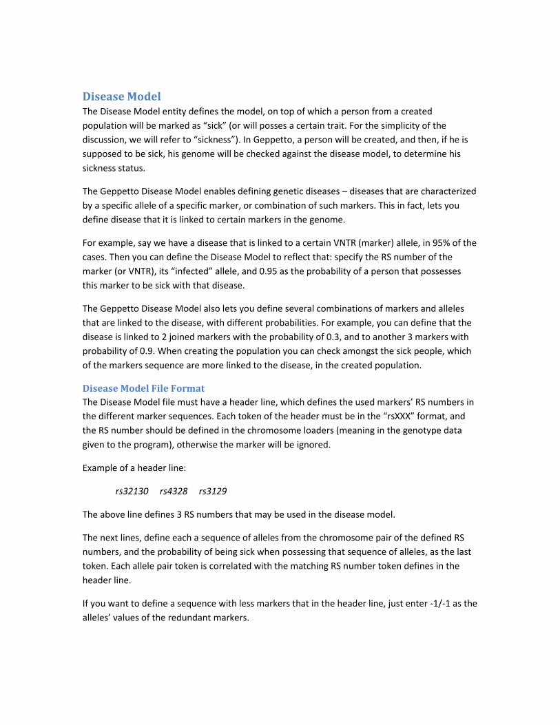
Disease Model File Format

The Disease Model file must have a header line, which defines the used markers’ RS numbers in

the different marker sequences. Each token of the header must be in the “rsXXX” format, and

the RS number should be defined in the chromosome loaders (meaning in the genotype data

given to the program), otherwise the marker will be ignored.

Example of a header line:

rs32130 rs4328 rs3129

The above line defines 3 RS numbers that may be used in the disease model.

The next lines, define each a sequence of alleles from the chromosome pair of the defined RS

numbers, and the probability of being sick when possessing that sequence of alleles, as the last

token. Each allele pair token is correlated with the matching RS number token defines in the

header line.

If you want to define a sequence with less markers that in the header line, just enter -1/-1 as the

alleles’ values of the redundant markers.

The disease model format also enables you to define only one allele value for a marker, when

the value of the other allele is not important. Set the unimportant allele value as -1.

Example of a sequence line:

a/c g/a t/t 0.9

The above line sets, that when a person has the alleles “a” and “c” at RS number rs32130 (from

both chromosomes), “g” and “a” at rs4328, and “t” and “t” at rs3129, that person has 0.9

probability of being sick.

Example of an entire Disease Model file:

rs32130 rs4328 rs3129

a/a a/a t/t 0.9

-1/-1 -1/-1 c/-1 0.3

Here there are 2 possible “causes” to the disease:

The first alleles sequence involves all the 3 markers defined in the header line, and it

causes the disease with probability of 0.9,

The second alleles sequence involves only 1 marker (the redundant markers in this

sequence are marked as having -1/-1 alleles), and the marker has only one allele that is

enough to cause sickness (if the genome contain the allele “c” in the marker rs3129,

while the other allele can have any value), and it causes the disease with probability of

0.3.

Pedigree File – PedFile The PedFile file format is a format used to describe a pedigree. A PedFile file describes all the

individuals in the pedigree (their sex, affected (sickness) status, etc.) and the family relations

between them – parenting relations, sibyl relations and etc.

The PedFile format Geppetto uses is adapted from the Superlink(SuperLink Genetic Linkage

Analysis Project n.d.) PedFile format, which is adapted from the Linkage PedFile format(Ped files

format n.d.) , with a minor addition that will be described.

PedFile Format

In this format, each individual in the pedigree is defined in a single line of text. The whole

pedigree is composed of individuals’ descriptions.

Each line has at least 10 fields. The mandatory fields:

In short:

Column 1: Pedigree number

http://cbl-fog.cs.technion.ac.il/superlink/


http://linkage.rockefeller.edu/soft/linkage/sec2.7.html


Column 2: Individual number

Column 3: Number of father

Column 4: Number of mother

Column 5: Number of first child

Column 6: Number of next sibling with same father

Column 7: Number of next sibling with same mother

Column 8: Sex - (1 = Male, 2 = female)

Column 9: ignored (the value must be 0)

Column 10: affected status - 1 is healthy, 2 is sick.

More detailed information:

1. Pedigree number. The pedigree number (ID) that the person is related to. There can

only be one pedigree in a PedFile.

2. Individual number. The person’s unique ID in the defined pedigree.

3. Father’s ID. The number of the person’s father in the pedigree. If the person does not

have a father in the defined pedigree, we consider the person as an “ancestor” of the

pedigree.

4. Mother’s ID. The number of the person’s mother in the pedigree. If the person does not

have a mother in the defined pedigree, we consider the person as an “ancestor” of the

pedigree.

5. Must exists, but the value is Ignored by the Geppetto program.



8. Sex. The person’s sex – set it to 1 if the person is a male, or 2 if female.

9. Must be of value 0.

10. Affected status: The person affected status determines if the person possesses the

sickness (or trait). Set it to 1 if the person is healthy (doesn’t posses the trait), 2 if the

person in sick (does posses the trait), or 0 if its condition is unknown (at this case, the

person will be treated as healthy).

Optional field supported in the Geppetto program is at field number 11 – The person’s

ancestry. To set the persons ancestry, add to the person line in the PedFile the field

“Pop:<ancestry>” when <ancestry> is A, B, … . If this value is not set, then the program will

treat the person as it is from the “A” population by default.

PedFile Example

The following is a PedFile which describes a pedigree with ID 2.

2 1 0 0 0 0 0 1 0 1 Pop:A

2 2 0 0 0 0 0 2 0 1 Pop:A

2 3 0 0 0 0 0 1 0 1 Pop:A

2 4 1 2 0 0 0 2 0 1 Pop:A

2 5 1 2 0 0 0 1 0 2 Pop:A

2 6 0 0 0 0 0 2 0 1 Pop:A

2 7 3 4 0 0 0 2 0 1 Pop:A

2 8 5 6 0 0 0 1 0 1 Pop:A

2 9 8 7 0 0 0 2 0 2 Pop:A

This PedFile describes the pedigree (male #5 and female #9 are sick, the pedigree if from

ancestry “A”):

Recombination Rate Producer Geppetto uses chromosome mixing as a way to simulate individual creation. In the process of

mixing, one chromosome naturally comes from the father and one from the mother. Before

they are transferred to the offspring, these chromosomes undergo the process of meiosis.

Geppetto simulates meiosis by simulating recombination events. According to Haldane, the

number of recombination events is a Poisson occurrence, distributed with a certain parameter

which is called the recombination rate parameter (Haldane 1919).

In order to reach high randomness, Geppetto uses a different recombination rate parameter for

every individual it produces. The way this is done is by raffling a different recombination rate

parameter each time. The distribution from which this parameter is taken depends on the user’s

input. Geppetto supplies a Normal distribution parameter producer, so the user can specify the

mean and variance of the normal distribution in the input file (see input sections of the different

scenarios for more information).

Geppetto offers the user an option to choose its own “meta-distribution” of the parameter.

Should they choose to do so, the users should implement the

IRecombinationRateProducer interface in package

Geppetto.metaRecombinationDistribution, and add it to the Geppetto class files when

running the program. There are 3 methods to implement:

1. int ProduceRecombinationRate() – this is the main method, in here you can

implement whatever distribution (or constant...) you wish for the recombination rate

parameter.

2. boolean QueryInterface(String descriptionLine) – This method queries

whether or not your interface matches the wanted parameters specified in the input

file. The parameter descriptionLine should be in the format: <Function> : <Parameters>

i.e. “Normal: 3, 0.5” for a Normal distribution with mean 3 and variance 0.5. Other than

that, you can name your interface whatever you want.

3. IRecombinationRateProducer CreateInstance(String descriptionLine,

long seed) – This method assumes that “QueryInterface” was called and succeeded.

It should initialize your object with the correct parameters according to the

descriptionLine accepted as a parameter. The seed parameter is used in case your class

uses a Random number generator as a member, so you can initialize it with the seed.

For further help on how to implement this feature, we advise you to check out the Geppetto source code and examine the implementation of the NormalRecombinationRateProducer class.

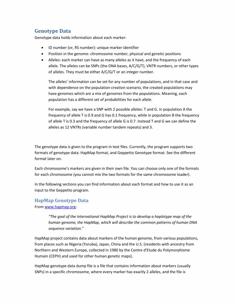
Genotype Data Genotype data holds information about each marker:

ID number (or, RS number): unique marker identifier

Position in the genome: chromosome number, physical and genetic positions

Alleles: each marker can have as many alleles as it have, and the frequency of each

allele. The alleles can be SNPs (the DNA bases, A/C/G/T), VNTR numbers, or other types

of alleles. They must be either A/C/G/T or an integer number.

The alleles’ information can be set for any number of populations, and in that case and

with dependence on the population creation scenario, the created populations may

have genomes which are a mix of genomes from the populations. Meaning, each

population has a different set of probabilities for each allele.

For example, say we have a SNP with 2 possible alleles: T and G. in population A the

frequency of allele T is 0.9 and G has 0.1 frequency, while in population B the frequency

of allele T is 0.3 and the frequency of allele G is 0.7. Instead T and G we can define the

alleles as 12 VNTRs (variable number tandem repeats) and 3.

The genotype data is given to the program in text files. Currently, the program supports two

formats of genotype data: HapMap format, and Geppetto Genotype format. See the different

format later on.

Each chromosome’s markers are given in their own file. You can choose only one of the formats

for each chromosome (you cannot mix the two formats for the same chromosome loader).

In the following sections you can find information about each format and how to use it as an

input to the Geppetto program.

HapMap Genotype Data From www.hapmap.org:

“The goal of the International HapMap Project is to develop a haplotype map of the

human genome, the HapMap, which will describe the common patterns of human DNA

sequence variation.”

HapMap project contains data about markers of the human genome, from various populations,

from places such as Nigeria (Yoruba), Japan, China and the U.S. (residents with ancestry from

Northern and Western Europe, collected in 1980 by the Centre d'Etude du Polymorphisme

Humain (CEPH) and used for other human genetic maps).

HapMap genotype data dump file is a file that contains information about markers (usually

SNPs) in a specific chromosome, where every marker has exactly 2 alleles, and the file is

http://www.hapmap.org/

population specific. That is, you can find genotype data about a chromosome for a specific

population.

The chromosome loaders accept HapMap genotype data dump (NOT the frequency or LD data

dump!) as the genotype data. You can obtain those files from the HapMap website, for example:

http://www.hapmap.org/genotypes/?N=D. You can specify several genotype data files, one for

each population. The chromosome loader must get also a genetic map, that maps the physical

positions of each marker to its genetic position on the chromosome (the HapMap genotype data

dump only contain information about the physical positions). This data also is accessible from

the HapMap website, and you can also find it here: https://mathgen.stats.ox.ac.uk/wtccc-

software/recombination_rates/. The program will match genetic positions from that map to the

HapMap genotype files, and will complete missing genetic distances when it can (by means of

simple interpolation).

HapMap Genotype File Format

In this file format, every line corresponds to a SNP – a marker with 2 alleles, and each file

represents one chromosome of a single population.

The line format (only describing the fields relevant to the Geppetto program):

1st field: marker ID, its RS number.

2nd field: chromosome number (“chr#” where # is between 1-22, or “chrX” for the X

chromosome, and “chrY” for the Y chromosomes – or “chr23” and “chr24” respectively).

3rd field: physical position of the marker on the chromosome. The position should be of

“long” type, meaning an positive integer number.

11th field: first allele value. The allele value is one of A/C/G/T.

12th field: first allele frequency.

14th field: second allele value.

15th field: second allele frequency. The frequencies should sum to 1, otherwise the

marker will be ignored by the chromosome loader.

You can read more about the HapMap genotype format in any of HapMap genotype data

READMEs, for example: http://www.hapmap.org/genotypes/latest_ncbi_build36/00README.txt

Note:

HapMap genotype files contain exactly 2 alleles per marker. So if you need more alleles

per marker, you might want to use the Geppetto genotype format.

Example:

Look at the following line from a chromosome 22 HapMap genotype file:

rs915674 chr22 14433624 + ncbi_b35 perlegen

urn:lsid:perlegen.hapmap.org:Protocol:Genotyping_1.0.0:2


http://www.hapmap.org/genotypes/?N=D


https://mathgen.stats.ox.ac.uk/wtccc-software/recombination_rates/


http://www.hapmap.org/genotypes/latest_ncbi_build36/00README.txt

urn:lsid:perlegen.hapmap.org:Assay:25760.6201814:1

urn:lsid:dcc.hapmap.org:Panel:CEPH-30-trios:1 QC+ G 0.871 101 A 0.129 15 116

The above line defines a marker (more specifically, a SNP) with RS number rs915674 on physical

position 14433624 at chromosome 22, with two alleles: G with frequency of 0.871 and A with

frequency 0.129.

How to Use HapMap Genotype Files

In order to run Geppetto with HapMap genotype files specify in the input file the following: For

each chromosome loader in the HapMap format, enter a line in the input file at the following

format:

#Genotype = <chrNumber>, <HapMap Genotype file path of population 1> < HapMap Genotype

file path of population 2>, <…>, <HapMap Genotype file path of population n>, <Genetic Map>

<chrNumber> is the chromosome number, an integer between 1..24 (23 is the X

chromosome, 24 is the Y chromosome),

There must be at least one HapMap genotype file, and the last file specified must be a

genetic map file (as explained earlier).

Example: #Genotype = 1, D:\Geppetto\ChrLoaders\allele_freqs_chr1_CEU_r21a_nr_fwd.txt, D:\Geppetto\ChrLoaders\allele_freqs_chr1_YRI_r21a_nr_fwd.txt, D:\Geppetto\ChrLoaders\genetic_map_chr1.txt #Genotype = 22, D:\Geppetto\ChrLoaders\allele_freqs_chr22_CEU_r21a_nr_fwd.txt, D:\Geppetto\ChrLoaders\allele_freqs_chr22_YRI_r21a_nr_fwd.txt, D:\Geppetto\ChrLoaders\genetic_map_chr22.txt The 2 lines above specify 2 chromosome loaders for the 1 and 22 chromosomes. There are 2 populations: CEU (Utah residents with ancestry from Northern and Western Europe) and YRI (Yoruban in Ibadan, Nigeria (West Africa)).

Geppetto Genotype Data In order to address HapMap genotype data downfalls, such as redundant fields for population

synthesis programs, lack of genetic distance data, its cumbersomeness, and the need to have

many files to describe markers of several ancestries, we defined a new genotype data format,

“Geppetto Genotype Data” format.

Geppetto genotype files are text files, where each marker is represented on a different, single

line of text.

It enables defining several alleles per marker, and several populations in a single file.

Geppetto Genotype File Format

Each line represents a marker. The line is separated into tokens, or fields, where each field is

separated by a space character(s) – series of single white spaces or tabs.

1st field: marker ID, its RS number.

2nd field: chromosome number (“chr#” where # is between 1-22, or “chrX” for the X

chromosome, and “chrY” for the Y chromosomes – or “chr23” and “chr24” respectively).

3rd field: physical position of the marker on the chromosome. The position should be of

“long” type, meaning a positive integer.

4th field: genetic position of the marker on the chromosome. The genetic position should

be of “double” type, meaning a positive fraction.

From the 5th field: here the different alleles of the marker are declared. All markers must

have the same number of alleles (if a marker has only one allele, or less alleles than it

should then enter bogus alleles to fill the fields, and set their frequencies to 0).

Each allele can be of type integer (useful for alleles of VNTR types for example), or a

genetic base, such as A/C/G/T.

Say we want to define n alleles at most per marker, then for each marker we will have n

fields for the alleles, we will mark them as a1, a2, …, an.

The next fields are the frequencies fields. Here are defined the frequencies of each allele

of the marker, per population.

If we have n alleles per marker, and p populations, then there must be n*p frequencies

fields.

Each population defines n frequencies, which match the alleles of the marker. The ith

population, will define the following allele frequencies: freqi(a1), freqi(a2), …, freqi(an).

The alleles’ frequencies for each population must sum up to 1.0.

See the example for another explanation.

Each frequency should be of type double, a number between 0.0 and 1.0, where you

must use “1.0” and “0.0” for 1 and 0, respectfully, in order to differentiate the

frequencies from the allele’s values.

Example:

Look at the following line from a Geppetto genotype file:

rs23 chr4 100 2.0; A G C; 0.2 0.7 0.1; 0.1 0.9 0.0; 0.0 0.0 1.0

The above line defines a marker in the Geppetto format. The marker RS number is 23, it is on

chromosome 4, in physical position 100, and genetic position 2.0. There are 3 alleles for the

marker: A, G and C, and there are 3 different populations defined.

In population 1 the frequency of allele A is 0.2, for G is 0.7, and for C is 0.1.

In population 2 the frequency of allele A is 0.1, for G is 0.9, and for C is 0.0 (This allele doesn’t

exist in population 2).

In population 3 the frequency of allele A is 0.0, for G is 0.0, and for C is 1.0 (in population 3, only

the C allele exists).

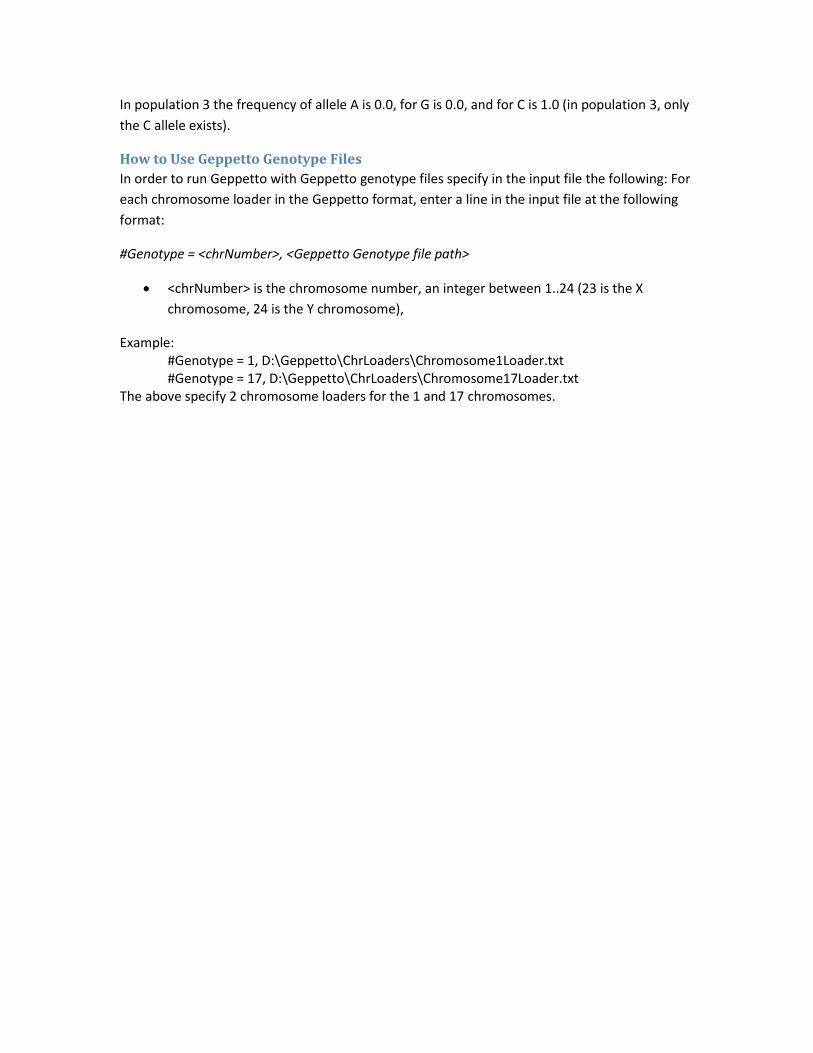
How to Use Geppetto Genotype Files

In order to run Geppetto with Geppetto genotype files specify in the input file the following: For

each chromosome loader in the Geppetto format, enter a line in the input file at the following

format:

#Genotype = <chrNumber>, <Geppetto Genotype file path>

<chrNumber> is the chromosome number, an integer between 1..24 (23 is the X

chromosome, 24 is the Y chromosome),

Example: #Genotype = 1, D:\Geppetto\ChrLoaders\Chromosome1Loader.txt #Genotype = 17, D:\Geppetto\ChrLoaders\Chromosome17Loader.txt The above specify 2 chromosome loaders for the 1 and 17 chromosomes.

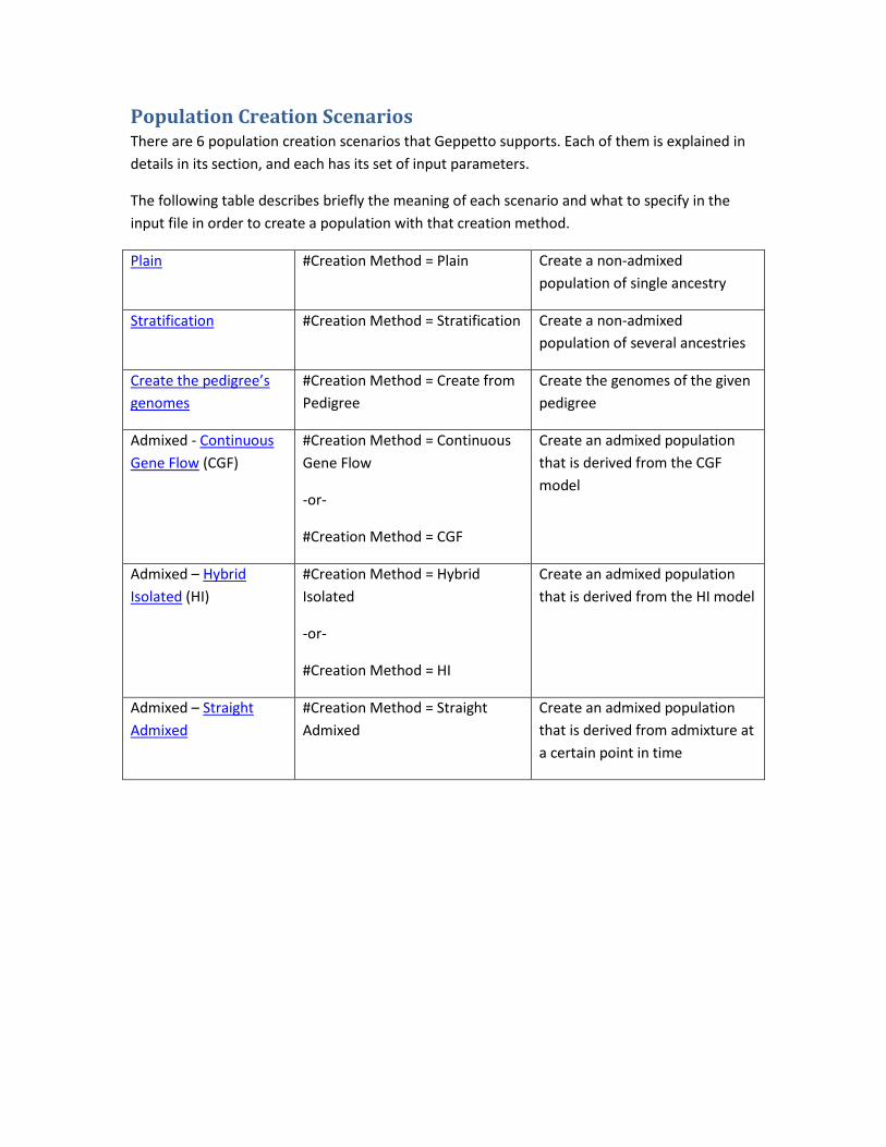
Population Creation Scenarios There are 6 population creation scenarios that Geppetto supports. Each of them is explained in

details in its section, and each has its set of input parameters.

The following table describes briefly the meaning of each scenario and what to specify in the

input file in order to create a population with that creation method.

Plain #Creation Method = Plain Create a non-admixed

population of single ancestry

Stratification #Creation Method = Stratification Create a non-admixed

population of several ancestries

Create the pedigree’s

genomes

#Creation Method = Create from

Pedigree

Create the genomes of the given

pedigree

Admixed - Continuous

Gene Flow (CGF)

#Creation Method = Continuous

Gene Flow

-or-

#Creation Method = CGF

Create an admixed population

that is derived from the CGF

model

Admixed – Hybrid

Isolated (HI)

#Creation Method = Hybrid

Isolated

-or-

#Creation Method = HI


that is derived from the HI model

Admixed – Straight

Admixed

#Creation Method = Straight

Admixed


that is derived from admixture at

a certain point in time

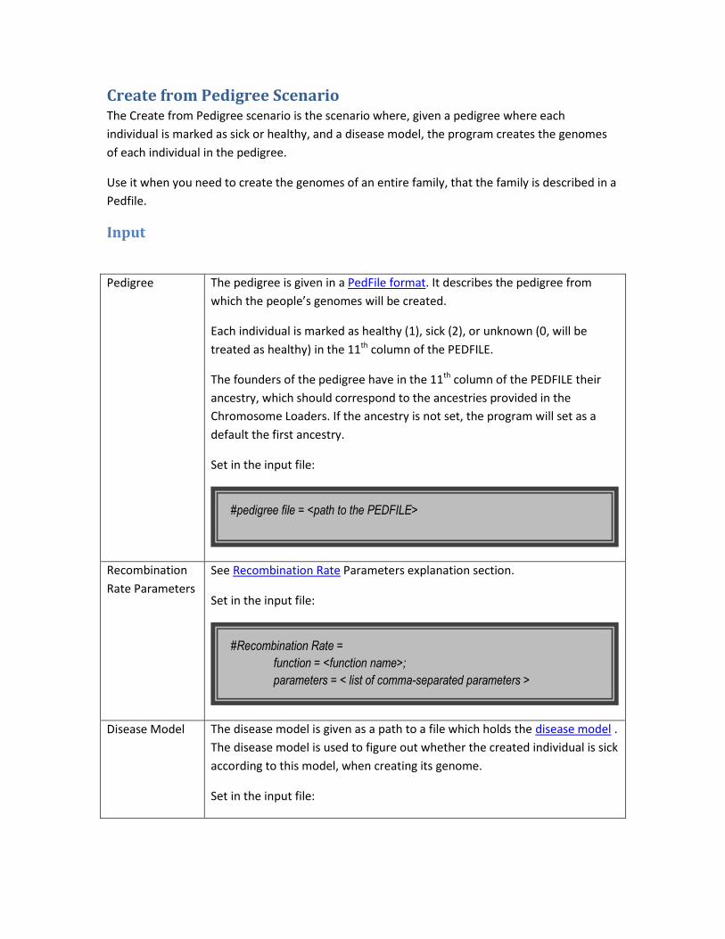
Create from Pedigree Scenario The Create from Pedigree scenario is the scenario where, given a pedigree where each

individual is marked as sick or healthy, and a disease model, the program creates the genomes

of each individual in the pedigree.

Use it when you need to create the genomes of an entire family, that the family is described in a

Pedfile.

Input

Pedigree The pedigree is given in a PedFile format. It describes the pedigree from

which the people’s genomes will be created.

Each individual is marked as healthy (1), sick (2), or unknown (0, will be

treated as healthy) in the 11th column of the PEDFILE.

The founders of the pedigree have in the 11th column of the PEDFILE their

ancestry, which should correspond to the ancestries provided in the

Chromosome Loaders. If the ancestry is not set, the program will set as a

default the first ancestry.


Recombination

Rate Parameters

See Recombination Rate Parameters explanation section.


Disease Model The disease model is given as a path to a file which holds the disease model .

The disease model is used to figure out whether the created individual is sick

according to this model, when creating its genome.


#Recombination Rate =

function = <function name>;

parameters = < list of comma-separated parameters >

#pedigree file = <path to the PEDFILE>

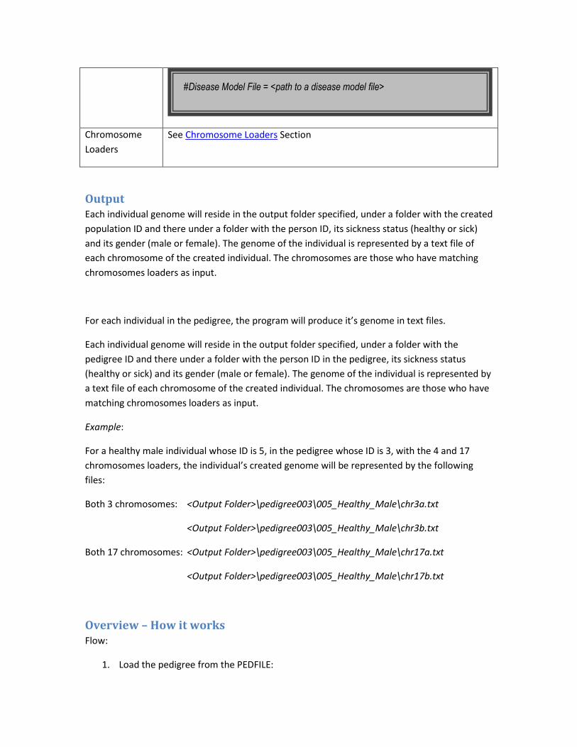
Chromosome

Loaders

See Chromosome Loaders Section

Output Each individual genome will reside in the output folder specified, under a folder with the created

population ID and there under a folder with the person ID, its sickness status (healthy or sick)

and its gender (male or female). The genome of the individual is represented by a text file of

each chromosome of the created individual. The chromosomes are those who have matching

chromosomes loaders as input.

For each individual in the pedigree, the program will produce it’s genome in text files.

Each individual genome will reside in the output folder specified, under a folder with the

pedigree ID and there under a folder with the person ID in the pedigree, its sickness status

(healthy or sick) and its gender (male or female). The genome of the individual is represented by

a text file of each chromosome of the created individual. The chromosomes are those who have

matching chromosomes loaders as input.

Example:

For a healthy male individual whose ID is 5, in the pedigree whose ID is 3, with the 4 and 17

chromosomes loaders, the individual’s created genome will be represented by the following

files:

Both 3 chromosomes: <Output Folder>\pedigree003\005_Healthy_Male\chr3a.txt

<Output Folder>\pedigree003\005_Healthy_Male\chr3b.txt

Both 17 chromosomes: <Output Folder>\pedigree003\005_Healthy_Male\chr17a.txt

<Output Folder>\pedigree003\005_Healthy_Male\chr17b.txt

Overview – How it works Flow:

1. Load the pedigree from the PEDFILE:

#Disease Model File = <path to a disease model file>

a. Parse each line of the PEDFILE, and create the pedigree structure.

b. Each node in the pedigree graph represents an individual in the pedigree.

2. Creating the genomes of each individual in the pedigree:

a. First, create the genomes of the founders.

Create each of the founder’s chromosomes, by assigning markers from the

markers data, according to his ancestry

b. For each two parents who their genomes are created, mate them to create their

child - mix their chromosomes, and create their child genome.

If their child should be sick, using the disease model, check whether the child’s

assigned genome has sick alleles. Try to mix the parents until the child’s genome

indicates a sickness according to the disease model. Do those until a certain

threshold – if it doesn’t work, return to step 1 for another try of creating a

pedigree that complies with the pedigree individuals’ status.

Create population from pedigree; Flow Diagram

Create Founders’

Genomes

For each individual,

that its parents are

created

Mate parents

Individual is sick (According to the

disease model)

Not sick

After enough tries,

start over Individual

is healthy

Individual is supposed

to be healthy

Individual is supposed

to be sick

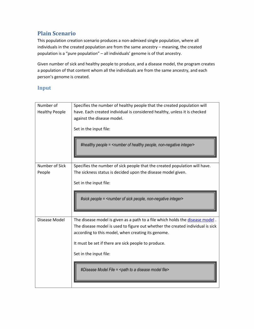
Plain Scenario This population creation scenario produces a non-admixed single population, where all

individuals in the created population are from the same ancestry – meaning, the created

population is a “pure population” – all individuals’ genome is of that ancestry.

Given number of sick and healthy people to produce, and a disease model, the program creates

a population of that content whom all the individuals are from the same ancestry, and each

person’s genome is created.

Input

Number of

Healthy People

Specifies the number of healthy people that the created population will

have. Each created individual is considered healthy, unless it is checked

against the disease model.


Number of Sick

People

Specifies the number of sick people that the created population will have.

The sickness status is decided upon the disease model given.





It must be set if there are sick people to produce.



#sick people = <number of sick people, non-negative integer>

#healthy people = <number of healthy people, non-negative integer>

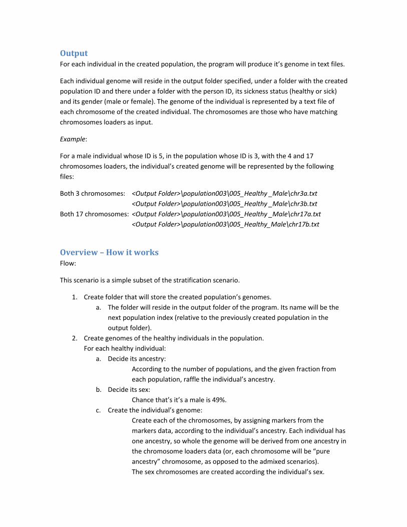
Output For each individual in the created population, the program will produce it’s genome in text files.

Each individual genome will reside in the output folder specified, under a folder with the created





Example:

For a male individual whose ID is 5, in the population whose ID is 3, with the 4 and 17


files:

Both 3 chromosomes: <Output Folder>\population003\005_Healthy _Male\chr3a.txt

<Output Folder>\population003\005_Healthy _Male\chr3b.txt


<Output Folder>\population003\005_Healthy_Male\chr17b.txt


This scenario is a simple subset of the stratification scenario.

1. Create folder that will store the created population’s genomes.

a. The folder will reside in the output folder of the program. Its name will be the

next population index (relative to the previously created population in the

output folder).

2. Create genomes of the healthy individuals in the population.

For each healthy individual:

a. Decide its ancestry:

According to the number of populations, and the given fraction from

each population, raffle the individual’s ancestry.

b. Decide its sex:

Chance that’s it’s a male is 49%.

c. Create the individual’s genome:

Create each of the chromosomes, by assigning markers from the

markers data, according to the individual’s ancestry. Each individual has

one ancestry, so whole the genome will be derived from one ancestry in

the chromosome loaders data (or, each chromosome will be “pure

ancestry” chromosome, as opposed to the admixed scenarios).

The sex chromosomes are created according the individual’s sex.

3. Create genomes of the sick individuals in the population.

For each sick individual:




b. Decide its sex:









d. Check if the created genome is sick according to the disease model:

Using the disease model, check whether the individual’s assigned genome has

sick alleles.

If it does, continue to create the next individual.

Else, try to create another individual, to replace current one. Do this until a

threshold of tries was achieved.

Stratification Scenario This population creation scenario produces a non-admixed population, where each person is of

different ancestry (the ancestries are user-defined) – meaning, of a different “pure population”,

and his entire genome is of that ancestry (or, “pure population” person).

Given number of sick and healthy people to produce, the fraction of each ancestry in the

created population, and a disease model, the program creates a population, in which the

number of people from each ancestry complies with the given population fraction, and each

person’s genome is created.

Use it when you need to create several people, each from several ancestries – might be useful

for genotype labeling testing – create a population of different ancestries and test whether the

labeling program labeled the genotype correctly.

It may be interesting to define a disease model, and then observed which of the ancestries are

most matched to the defined disease model – Say that there are 2 populations, A and B, and the

fraction of each population is 50%, and 90% of the created sick individuals are originated in

population A, then we can fairly deduct that the disease model is depicting a population A

related disease.

Input

Number of

Populations

Specifies the number of populations that the created population’s

individuals are composed from. Meaning, each original population will be

treated as an ancestry, and the first population will be marked as ancestry of

type “A”, the second will be marked as “B” and so on. The ancestries

marking should comply with the ancestries given in the chromosome loaders

files.

Each created individual from the created population will have a genome that

is composed solely of one ancestry.


Fraction of Each

Population

Specifies the fractions of each original population representation in the

created population. The number of fractions must be the same of the

number of population specified (see above parameter), and must sum up to

one - as each created individual has origin from exactly one original

population.

#Number of populations= <number of populations, non-negative integer>

For example, to create a population that is comprised from 2 different

populations (or ancestries), that is comprised of 80% individuals from the

first original population, set the population fractions to 0.8; 0.2


Number of

Healthy People




The healthy people can be of any of the original ancestries.


Number of Sick

People



The sick people can be of any of the original ancestries. This may be

interesting to test the relevance and connection of a certain disease model

to an original population.









#PopFreq = <semi-colon delimited list of fractions that sum to 1>







Example:

For a healthy male individual whose ID is 5, in the population whose ID is 3, with the 4 and 17


files:

Both 3 chromosomes: <Output Folder>\population003\005_Healthy_Male\chr3a.txt

<Output Folder>\population003\005_Healthy _Male\chr3b.txt


<Output Folder>\population003\005_Healthy_Male\chr17b.txt





output folder).






b. Decide its sex:










3. Create genomes of the sick individuals in the population.

For each sick individual:




b. Decide its sex:









d. Check if the created genome is sick according to the disease model:

Using the disease model, check whether the individual’s assigned genome has

sick alleles.




Admixed Populations Scenarios These population creation scenarios produce populations of admixed individuals. An admixed

individual is a person whose ancestral origin relies on more than one pure ancestry. For

example, African Americans are the consequence of an admixture of two “pure” populations –

Europeans and Africans.

Geppetto population synthesis program currently supports 3 admixed population creation

scenarios:

Hybrid Isolated, Continuous Gene Flow and Straight Admixed.

Hybrid Isolated Scenario In this model of admixture(Pfaff, et al. 2001), the populations are assumed to have mixed at

some point in history, and blended into one another in a way that mating was free between

individuals from different populations. Hence, the mixture occurs over a span of one generation,

and the next generation consists of admixed individuals, who have large ancestral segments of

DNA in their chromosomes, and breed among themselves. As the generations advance and time

elapses, the segments of ancestral DNA in the chromosome become shorter until they reach a

point where the information extracted from this data does not contribute what is expected from

MALD. Therefore, we recommend the user not to create a population in this model with an

admixture that occurred over 15 generations ago.

Input

Number of

Healthy People





Number of Sick

People




Disease Model The disease model is given as a path to a file which holds the disease model.








Number of

Generations

The number of generations that passed since the populations were first

introduced.


Number of

Populations

The number of populations that admixed together. See the part on ”How

Does the number of populations blend in?” for further information.


Populations

Fractions

The fractions of each of the populations in the genome of the admixed

individual. The number of values supplied must be equal to the number of

populations specified. In addition, the fractions must sum to 1. In CGF, the

first value will be the fraction of the main population. See the part on “How



For example:

Recombination

Rate Parameters



#populations fractions = 0.5 ; 0.3 ; 0.1 ; 0.1

#populations fractions = <fraction> ; <fraction> ; <fraction>; ...

#number of populations = <number of populations, non-negative integer>

#Generations = <number of generations, non-negative integer>







Inside the person’s folder you will also find a PedFile that describes the pedigree that created

that individual, and a folder named “Ancestors” that lists the chromosomes of the people in the

pedigree (who are that person’s ancestors). An interesting point is examining the chromosomes

of the people in the pedigree from the top level to the bottom and seeing how the ancestral

segments become a more and more delicate partition of the chromosome.

Example:



files:


<Output Folder>\population003\005_Healthy_Male \chr3b.txt

Both 17 chromosomes: <Output Folder>\population003\005_Healthy_Male \chr17a.txt


Ped file: <Output Folder>\population003\005_Healthy_Male \ancestors.ped

Ancestors’ chromosome files (example for ancestor number 4, female):

<Output Folder>\population003\005_Healthy_Male \Ancestors\004_Healthy_Female.txt

Overview – How It Works The method of creating each individual is by simulating the pedigree that created him/her.

Given the parameters listed above, a person from the admixed population has a pedigree that is




predicted by the program, and, starting from the founders of the pedigree, mating is simulated

to form the final offspring, who is the admixed individual.

How does the number of populations blend in?

For each individual there is a pedigree that creates him/her. In this model of admixture, the

pedigree is an inverse full tree, with the founders all at the top level. They are assigned

populations randomly according to the population fractions from the input file.

Flow:




output folder).


For each individual:

a. Decide its sex:


b. Raffle the pedigree that creates him/her:

According to the admixture model, gender, number of populations, and

the given fraction from each population. For sick people, create the

pedigree such that the offspring of the pedigree will have a sick status.


Assign the people in the pedigree their genomes. Pay attention, that for

each of the people in the pedigree, the chromosomes will only contain

the ancestral segments. Making use of the chromosome loader files will

only take place for creating the actual individual that belongs to the

population.

Continuous Gene Flow Scenario In this model (Pfaff, et al. 2001), there is one dominant population that is breeding among itself.

At a certain point in time, other populations (possibly more than one) started mingling with this

population, to insert a certain amount of genetic information into the population. In every

generation, a fixed average percentage, α, of foreign DNA is assumed to have been “injected”

into the population. With time, the percentage of the injected population’s DNA will increase

within the admixed population’s individuals’ chromosomes.

Input

Number of

Healthy People





Number of Sick

People









Number of

Generations

The number of generations that passed since the populations were first

introduced.





Number of

Populations

The number of populations that admixed together. See the part on ”How



Populations

Fractions



populations specified. In addition, the fractions must sum to 1. In CGF, the

first value will be the fraction of the main population. See the part on “How



For example:

Recombination

Rate Parameters









#Generations = <number of generations, non-negative integer>







Inside the person’s folder you will also find a PedFile that describes the pedigree that created

that individual, and a folder named “Ancestors” that lists the chromosomes of the people in the

pedigree (who are that person’s ancestors). An interesting point is examining the chromosomes

of the people in the pedigree from the top level to the bottom and seeing how the ancestral

segments become a more and more delicate partition of the chromosome.

Example:



files:





Ped file: <Output Folder>\population003\005_Healthy_Male \ancestors.ped

Ancestors’ chromosome files (example for ancestor number 4, female):

<Output Folder>\population003\005_Healthy_Male \Ancestors\004_Healthy_Female.txt

Overview – How It Works The method of creating each individual is by simulating the pedigree that created him/her.

Given the parameters listed above, a person from the admixed population has a pedigree that is

predicted by the program, and, starting from the founders of the pedigree, mating is simulated

to form the final offspring, who is the admixed individual.

How Does the number of populations blend in?

For each individual there is a pedigree that creates him/her. In this model of admixture, the

pedigree is created dynamically, from offspring to founders. According to population fractions

and the number of generations, the pedigree is created. The founders located at the top level

will be from the main population, and every founder that arrived later will have an ancestry of

one of the co-populations. The main population is always considered “population A”, so in the

population fractions part in the input file, the first value should be the fraction of the main

population, and the rest of the values will be the fractions of the co-populations.

Flow:




output folder).


For each individual:

a. Decide its sex:


b. Raffle the pedigree that creates him/her:

According to the admixture model, gender, number of populations, and

the given fraction from each population. For sick people, create the

pedigree such that the offspring of the pedigree will have a sick status.


Assign the people in the pedigree their genomes. Pay attention, that for

each of the people in the pedigree, the chromosomes will only contain

the ancestral segments. Making use of the chromosome loader files will

only take place for creating the actual individual that belongs to the

population.

Straight Admixed Scenario This population creation scenario produces a population of admixed individuals. An admixed

individual is a person whose ancestral origin relies on more than one pure ancestry. For

example, African Americans are the consequence of an admixture of two “pure” populations –

Europeans and Africans.

This scenario provides an additional method to create admixed populations. It will be interesting

for the user to create several populations using the different scenarios and models of admixture

and examine the differences in the created individuals (interesting parameters: size of

segments, their distribution, the ancestral distribution of segments, the ancestry at the disease

locus which cause for the sickness status, etc.).

The method of creation for this scenario is as the name implies. In contradiction to the previous

scenario, in which the individual was created by simulating the actual admixture of its ancestors,

in this scenario the person is created in a straight forward way by creating its admixed

chromosomes. The creation of admixed chromosomes is done as a simulation according to

parameters that describe the admixture pattern of the populations (Patterson, et al. 2004).

There are two important parameters which influence the outcome of an admixed chromosome

creation:

1. Lambda parameter: this parameter simulates the number of generations that passed

since admixture. The higher it gets, the more delicate will be the partition of the

chromosome to ancestral segments, i.e. there will be more segments and they will be

shorter.

In our program, this parameter is believed to be distributed with Gamma

distribution(Patterson, et al. 2004) across individuals in the population. Therefore, in the

input file, the user must supply a mean and variance for this parameter, and for each

individual there will be a randomization of the specific lambda parameter according to

the parameters supplied.

How this parameter is used:

Actually, ancestral segments in the chromosome are the result of recombination events

that occur in meiosis. Recombination rate is often modeled as a Poisson process, which

means that the number of recombination events is Poissonly distributed. In addition, as

a general property of Poisson processes, the length of the segments is distributed

exponentially. So the lambda parameter is used as the parameter of an Exponential

distribution in randomizing segment lengths.

2. Populations Fractions: this parameter indicates what the fraction of each population is

in the genome of the created individual. For example, a common fraction is used is for

African Americans, who are believed to be composed of 0.8 African ancestry and 0.2

European Ancestry.

Input

Number of

Healthy People





Number of Sick

People









Lambda

parameter

The lambda parameter’s mean and variance. See the paragraph on “Lambda

parameter” for further information.


Number of The number of populations that admixed together.

#Lambda = <mean> ; <Variance>




Populations Set in the input file:

Populations

Fractions



populations specified. In addition, the fractions must sum to 1.


For example:

Recombination

Rate Parameters









Example:









files:





Overview – How It Works Flow:




output folder).



a. Decide its sex:


b. Divide its chromosome to segments

According to the lambda parameter, creates a partition of the

chromosome to segments. Each segment is decided its ancestral origin

randomly in accordance with the population fractions parameter.

c. Create the individual’s genome: Each marker is given its allele value according to the ancestry of the segment in which it relies, and to the frequencies of alleles specified in the chromosome loader file.

For each sick individual: a. Decide its sex:


b. Divide its chromosome to segments

According to the lambda parameter, creates a partition of the

chromosome to segments. Each segment is decided its ancestral origin

randomly in accordance with the population fractions parameter.

c. Create the individual’s genome: Each marker is given its allele value according to the ancestry of the segment in which it relies, and to the frequencies of alleles specified in the chromosome loader file.

d. Check if the created genome is sick according to the disease model: Using the disease model, check whether the individual’s assigned

genome has sick alleles.




References HapMap Project:

Home: http://www.hapmap.org/.

Genotype data files: http://www.hapmap.org/genotypes/?N=D

Genetic Maps: https://mathgen.stats.ox.ac.uk/wtccc-software/recombination_rates/

README: http://www.hapmap.org/genotypes/latest_ncbi_build36/00README.txt

SuperLink Software: http://cbl-fog.cs.technion.ac.il/superlink/.

Ped File Format: http://linkage.rockefeller.edu/soft/linkage/sec2.7.html.

AncestryMap Software: http://genepath.med.harvard.edu/~reich/Software.htm.

Haldane, J.B.S. "The combination of Linkage values and the calculation of distances between the

loci of linked factors." Journal of Genetics 8 (1919): 299-309.

Patterson, N, et al. "Methods for high-density admixture mapping of disease genes." American

Journal of Human Genetics 74, no. 5 (May 2004): 1001-1013.

Pfaff, C. L., et al. "Population Structure in Admixed Populations: Effect of Admixture." American

Journal of Human Genetics, no. 68 (2001): 198-207.


http://www.hapmap.org/genotypes/?N=D


http://www.hapmap.org/genotypes/latest_ncbi_build36/00README.txt



http://genepath.med.harvard.edu/~reich/Software.htm

Documents

Geppetto – Population Synthesis Software