Geophysical Journal International - UMR 8538madariag/Papers/Twardzik_Parkf.pdf · Geophysical Journal International Geophys. J. Int. (2012) doi: 10.1111/j.1365-246X.2012.05653.x GJI

Geophysical Journal InternationalGeophys. J. Int. (2012) doi: 10.1111/j.1365-246X.2012.05653.x

GJI

Sei

smol

ogy

Robust features of the source process for the 2004 Parkfield,California, earthquake from strong-motion seismograms

C. Twardzik,1 R. Madariaga,2 S. Das1 and S. Custodio3

1Department of Earth Sciences, University of Oxford, Oxford, United Kingdom. E-mail: [email protected] de Geologie, Ecole Normale Superieure, Paris, France3Centro de Geofısica, Faculdade de Ciencias e Tecnologia da Universidade de Coimbra, Coimbra, Portugal

Accepted 2012 August 15. Received 2012 July 25; in original form 2011 December 23

S U M M A R YWe explore a recently developed procedure for kinematic inversion based on an ellipticalsubfault approximation. In this method, the slip is modelled by a small set of elliptical patches,each ellipse having a Gaussian distribution of slip. We invert near-field strong ground motionfor the 2004 September 28 Mw 6.0 Parkfield, California, earthquake. The data set consists of 10digital three-component 18-s long displacement seismograms. The best model gives a momentof 1.21 × 1018 N m, with slip on two distinct ellipses, one with a high-slip amplitude of 0.91 mlocated 20 km northwest of the hypocentre. The average rupture speed of the rupture processis ∼2.7 km s−1. We find no slip in the top 5 km. At this depth, a lineation of small aftershocksmarks the transition from creeping above to locked below, in the interseismic period. The high-slip patch coincides spatially with the hypocentre of the 1966 Mw6.0 Parkfield, California,earthquake. The larger earthquakes prior to the 2004 Parkfield earthquake and the aftershocksof the 2004 earthquake (Mw > 3) also lie around this high-slip patch, where our model imagesa sharp slip gradient. This observation suggests the presence of a permanent asperity thatbreaks during large earthquakes, and has important implications for the slip deficit observedon the Parkfield segment, which is necessary for reliable seismic hazard assessment.

Key words: Inverse theory; Earthquake dynamics; Earthquake ground motions; Earthquakesource observations; Seismicity and tectonics; Continental tectonics: strike-slip and transform.

1 I N T RO D U C T I O N

The aim of inversions for the earthquake source process is to findthe slip distribution history that produces the best fit to the recordedground motion. The usual approach in kinematic inversions is tosubdivide the fault plane into rectangular subfaults, an approachfirst taken by Trifunac (1974). In each of these subfaults, sourceparameters are then retrieved. However, this approach has the dis-advantage of requiring a large number of subfaults to adequatelymodel the fault plane, introducing non-uniqueness into the problem(Das & Kostrov 1990, 1994), which is dealt with by using additionalconstraints. In this paper, we investigate a recently developed pro-cedure for kinematic inversion involving elliptical subfaults, which,in addition to creating an intrinsically smooth slip distribution in-side the slipping region, has the advantage of reducing the numberof parameters to be inverted for. We use only a small number ofellipses, each of which is described by seven parameters. To testthis approach with near-field records, we analyse the strong-groundmotion data for the 2004 September 28 Mw6.0 Parkfield, Californiaearthquake to obtain its robust source features.

The Parkfield segment is part of the San Andreas transform faultsystem which accommodates right-lateral tectonic motion between

the Pacific (PAC) and the North-American (NAM) plates (Fig. 1).Bounded by a creeping section to the northwest and a locked sectionto the southeast (the Cholame segment), this region experienced fiveearthquakes of about Mw6.0 since 1881 (e.g. Bakun & McEvilly1979; Toppozada et al. 2002; Smith & Sandwell 2006). Knowledgeof the occurrence of the 1934 and the 1966 Parkfield earthquakesand the suggestion that the 1966 earthquake was an almost exactrepeat of the 1934 earthquake, led to the setting up of the ParkfieldPrediction Experiment (Bakun & Lindh 1985). As a consequence,the 2004 earthquake at Parkfield was widely recorded by seismic aswell as other types of instruments.

The data set used here consists of 10 digital three-componentstrong-motion displacement seismograms with a duration of 18 s.Six stations are located on the northeastern side of the fault andfour stations are on the southwestern side (Fig. 1). In addition, thereare also 33 analogue stations that recorded this earthquake. The useof digital stations has two advantages: first, they have absolute tim-ing, and secondly, the first P-wave arrival is recorded. Though wedo not use data from analogue stations for the inversions, we shalluse them later for a cross-check on our model by calculating thedisplacements at those stations and examining how well the wave-forms are matched. All the displacement records were bandpass

C© 2012 The Authors 1Geophysical Journal International C© 2012 RAS

2 C. Twardzik et al.

Figure 1. Tectonic setting and station distribution for the 2004 September 28 Mw6.0 Parkfield, California, earthquake. The digital stations (GEOS network,Borcherdt et al. 1985) are shown as red triangles, whereas the blue triangles represent available analogue stations (CGS network). The fault trace used for theinversions is shown by the thick black line; the grey lines show the surface expression of the San Andreas Fault. The ‘beach ball’ is connected by a thin line tothe earthquake epicentre. Start time of each trace is the origin time of the earthquake.

filtered between 0.16 and 1 Hz. The lower frequency limit is chosenbased on the instrument capability of analogue stations. Though thelower frequency limit for the digital stations could be taken down to0.1 Hz, we used 0.16 Hz to keep consistency between different datasets. The higher frequency limit is determined by the accuracy ofthe velocity structure and Green’s functions (Liu et al. 2006).

2 K I N E M AT I C I N V E R S I O N M E T H O D

We model the fault as a rectangular plane, 40 km long (30 km tothe northwest and 10 km to the southeast of the hypocentre) and16 km wide along depth, its surface projection being shown as astraight black line on Fig. 1. The size of the fault is based on thelocation of the aftershocks that occurred within 24 hr of the mainshock; strike and dip are taken as N140E and 87◦, respectively;hypocentral location is 35.82◦N, 120.37◦W, at a depth of 8.3 km(Thurber et al. 2006). The velocity model used for the computationof Green’s functions is the 1-D structure used by Liu et al. (2006).

The method of elliptical subfault approximation has been usedfor kinematic inversions by Vallee & Bouchon (2004), Peyrat et al.(2010) and Di Carli et al. (2010). In this approach, each ellipticalpatch is defined by the seven parameters shown in Fig. 2. In eachellipse, the slip distribution has a smooth Gaussian distribution fromthe maximum slip amplitude at the centre to zero slip amplitude atboundaries. We require that the first ellipse contains the hypocentre.The centre of the ellipse is calculated using two parameters: hr

and αh, which control the position of the ellipse relative to thehypocentre. αh is the azimuth of the centre of the ellipse about thehypocentre; hr is the distance between the hypocentre and the centreof ellipse (this distance cannot be greater than the length of thesemi-major axis). For the first ellipse, the rupture time is calculatedassuming a circular rupture front, starting from the hypocentre att = 0, and propagating at the rupture speed associated with the firstellipse (This rupture speed is one of the parameters we invert for).

Figure 2. Description of the elliptical subfault patches (based on Vallee &Bouchon 2004). Each patch can be described by the following parameters:(x0,y0): the two coordinates of the ellipse centre. (xa,xb): size of semi-majorand semi-minor axes, respectively. α: angle between the semi-major axisand the horizontal. smax: maximum slip. The slip distribution (S) inside

each ellipse is defined as: S(x, y) = smaxexp [−( x2

x2a

+ y2

x2b

)]. vr: the rupture

velocity within each ellipse.

The rupture of the second ellipse is initiated at the point where thecircular rupture front, from the hypocentre, makes its first contactwith the ellipse. To determine the time when the second ellipsestarts rupturing, we calculate the time needed to travel from thehypocentre to the initiation point with the rupture speed of thesecond ellipse. This rupture speed is also a parameter inverted for.The same process is repeated for other ellipses, when used.

The complete wavefield Green’s functions, including near-fieldterms, are computed over the fault using 500 m × 500 m cellsizes, using the AXITRA code (Cotton & Coutant 1997), whichcombines the reflectivity method (Kennett & Kerry 1979) with thediscrete wavenumber decomposition (Bouchon 1981). The samecode is used to simulate the wave propagation and compute solutionseismograms.

During an inversion, the aim is to minimize a cost function. Thisfunction measures the difference between observed data (uo) and

C© 2012 The Authors, GJI

Geophysical Journal International C© 2012 RAS

Source process of the Parkfield earthquake 3

modelled seismograms (us). For our study, we choose the followingcost function (Spudich & Miller 1990):

E =Nd∑i=1

Wi

( ∑tetb

(uoi (t) − us

i (t))2∑te

tb(uo

i (t))2 + ∑tetb

(usi (t))

2

). (1)

In eq. (1), W i is the weight given to each station. A higher weightis given to stations with a high signal-to-noise ratio, with valueschosen as in Liu et al. (2008). Nd is the number of records and(tb, te) gives the beginning and end times. The search algorithmfor the best parameters used in this paper is the neighbourhoodalgorithm (Sambridge (1999a,b), which simultaneously searchesfor the best values of the parameters. This algorithm obeys thefollowing reasoning: The first step is to uniformly sample ni modelsinside the parameter space. The seismograms are then computedfor each model, and a misfit value is found for each, using the costfunction (ε). nr models with the smallest misfit are then selectedfrom the initial ni models. According to the distribution of thosenr models, a Voronoi diagram (Voronoi 1908) is built, where eachmodel is associated with a Voronoi cell. A new set of ni models inthe regions defined by the Voronoi cells is then sampled.

Initially, tests were performed using artificially constructed datato obtain better insight into the method of inversion, for variouscases (see Appendix). In particular, in ‘Test 3’, we address thequestion of the number of ellipses to be used, when no previousstudy of the earthquake exists.

During each inversion, we choose to fix two source parameters:the rise-time (τ ) and the rake, constant over the entire fault. Dueto the range of frequencies used in this study, the rise-time maynot be resolvable (Liu et al. 2006). Based on a previous kinematicinversion and dynamic modelling, we choose a value of 0.5 s for τ

(Liu et al. 2006); (Ma et al. 2008). Previous studies also show thatthe rake angle does not have large fluctuations, so it is reasonable toassume the rupture to be purely right lateral (Custodio et al. 2009).

3 C H O I C E O F T H E P R E F E R R E D M O D E L

We performed 12 inversions using different parameters to find thesource process for the 2004 Parkfield earthquake (see SupportingInformation Table S1). Fig. 3 shows the final slip distributions for the12 inversions and Table S1 gives details of the different inversions,and the resulting source processes. For 11 inversions, two ellipseswere used, and one case with three ellipses is also considered. Thechoice of two ellipses was based on the slip distributions inferredfrom other studies of this earthquake, using different methods (e.g.Murray & Langbein 2006; Allmann & Shearer 2007; Ma et al.2008). For some of the inversions, we also required the secondellipse to be connected to the first one. In that case, (hr, αh) relate tothe centre of the first ellipse, rather than to the hypocentre. We alsocarry out some inversions in which we vary the rise-time (τ ) and therake to examine their influence on the solutions. In addition to that,two inversions using only analogue stations were also carried outand are reported in Sections S14– S15 of the Supporting InformationS2. We discuss next the choice of our preferred model among theseinversions.

Fig. 3 shows that several models have similar misfits, and thisleads to the problem of selection of the preferred solution. In spiteof the diversity, we find that there is consistency between the mod-els. To highlight the robust features which are independent of thechoice of a priori conditions (Table S1), a simple average of allthe models, inversely weighted by the misfit value, is plotted in

Figure 3. Final slip distribution (m) for the 12 inversions (see Supporting Information Table S1 for details), using digital stations. The misfit E is given in thetop right of each fault. The red star shows the position of the hypocentre. The preferred model is highlighted by the red rectangle.




Figure 4. Average slip distribution (m) for the 12 slip models. The starshows the position of the hypocentre. The region within the black line showsslip which is higher than the standard deviation.

Fig. 4. In Fig. 4, we shade regions of slip which are smaller thanthe standard deviation calculated over the 12 inversions. Therefore,the remaining area focuses on the robust features extracted from the12 inversions. The misfit of 0.35 for this average model (calculatedassuming a constant rupture velocity of 3.0 km s−1), falls withinthe range of values obtained for the 12 inversions, showing that thefeatures highlighted by this averaged slip distribution does not leadto a non-realistic model. On average, two slip patches are necessaryto explain the data, one close to the hypocentre and a second onelocated between 15 and 20 km northwest of the hypocentre, with noslip in the top 5 km. This suggests that the slip distribution of thepreferred model should include these properties. It is also importantto note that we find a strong resemblance with previous models ofthis earthquake, obtained from analysis of strong motion data butusing different inversion methods (Ma et al. 2008); Custodio et al.(2009). This indicates that the main features are independent of theapproach used to find the slip distribution.

As we also invert for the rise-time and the rake in some of theinversions, it is interesting to discuss their influence on the obtainedsolutions. The rake varies between 140 and 180◦ in all the inver-sions, with a constant value over the entire fault. This is consistentwith the results of Liu et al. (2006) showing that some parts ofthe fault exhibits a combined right-lateral and reverse motion. Therise-time shows a higher variability, making it difficult to discussthe reliability of the results. However, it is interesting to see thatInversions 6 and 8 show a similar final slip distribution with dif-ferent values for the rise time (see Tables S6 and S8 in SupportingInformation S2).

This implies that this parameter cannot be resolved, and thereforeits impact on the final solution may not be significant. Of the 12 in-versions, eight have significant slip at the hypocentre (Inversions 2,3, 5, 6, 8, 9, 10, 12—see Fig. 3). Among these eight, only Inversion5 does not have a high-slip patch northwest of the hypocentre. Ifwe also require the preferred model to have a moment value within±15 per cent of the CMT value (i.e. between 0.96 × 1018 and1.30 × 1018 N m), then of the remaining seven models, only Inver-sions 2, 6, 8 and 10 satisfy this condition. We may reject Inversion2 from the list of acceptable models, due to the fact that the rup-ture speed in the first ellipse exceeds the shear wave speed at thehypocentral depth by ∼30 per cent, and no previous study found su-pershear rupture speed for this earthquake (e.g. Fletcher et al. 2006,and others referred earlier). Finally, by generating the seismogramsat the analogue stations for the three remaining models, we calcu-late the values of the misfit for digital stations and analogue stationstogether. Since Inversion 6 has the lowest global misfit (0.82, with0.26 and 0.56 for digital and analogue records, respectively) we takeit as our preferred model.

4 D I S C U S S I O N O F T H E P R E F E R R E DM O D E L

Fig. 5 shows the comparison of the waveform data generated by thepreferred model with the seismograms recorded at the 10 digitalstations. We see that the seismograms show an excellent matchin the wave shape and an excellent timing for the main pulses.In general, the amplitude is very well retrieved in the early partof the record, though we note that the later arrivals are not wellfitted. It has been known for some time (Li et al. 1990); Ben-Zion(1998) that waves from the fault zone gouge exist and could havea strong effect on the recorded strong-ground motion (Fukushimaet al. 2010). The deterioration of the agreement between the dataand the solution seismograms in the later portions of the record atsome stations may stem from the fact that these fault-zone wavesare not modelled in our study. The same reason could also explainthe mismatch in amplitude in the early part of some stations (e.g.MFU), situated very close to the fault.

Fig. 6 shows the comparison between waveform data and thepreferred model solution seismograms at the 33 analogue stations.In the forward direction of rupture propagation (i.e. northwest fromthe hypocentre), a good agreement is observed only for the mainpulses. In the backward direction, waveforms at some stations arenot well matched. To have a more quantitative view of this mismatch,we plot the misfit values at all the analogue stations separately for ourpreferred model (Fig. 7a). The red dashed line represents the meanof the individual misfit value, so we can consider that stations abovethis line exhibit a significant mismatch. We identified three locationsof higher mismatch (Fig. 7b), one at the extreme northwestern end ofthe fault (Station COAL), one near the region of the high-slip patch(Stations FZ12, FZ15, VC1W, VC2W, VC3W and VC5W) and onein the southeastern end of the fault (Stations FZ1, C1E, CH2W andCH3W). It is interesting to see that most of these stations are veryclose to the fault, which is a propitious area to be influenced byfault zone trapped waves (e.g. Li et al. 2004), and could explainthe high amplitude and the highest mismatch between observedand calculated seismograms at those stations. For stations closeto the high-slip patch, we believe that this area which released asignificant amount of the total energy during the earthquake, couldhave resulted in enhanced site effects, which could explain thehigher mismatch for stations at larger distances to the fault.

Previous models using seismic data (e.g. Allmann & Shearer2007; Custodio et al. 2009) as well as our study have some slip atthe hypocentre. A study of the Parkfield earthquake using geodeticdata (InSAR and GPS) by Johanson et al. (2006), has argued thatslip at hypocentre may be due to rapid after-slip. Hypocentral slipmay only be needed to explain the large amplitude observed atanalogue stations FZ1, C1E and C2W (see Fig. 6), as also pointedout earlier (e.g. Shakal et al. 2006). Also, some of our inversionseither have no slip or, no significant slip at hypocentre (Inversions1, 4, 5, 7 and 11). Among these, Inversions 1, 5 and 9 explain thesignal observed at analogue stations even better than our preferredmodel. To test if some slip at the hypocentre is a source signal oran artefact induced by fault zone waves affecting stations at thesoutheastern extremity of the fault, we run an inversion using alldigital and analogue stations, except FZ1, C1E, CH2W and CH3W,which have significantly larger misfit, and the same set-up as inInversion 6. The resulting slip distribution (Fig. 7c), shows thateven without these high-misfit stations, which also have very highamplitudes, some slip at the hypocentre is needed to explain thedata.




Figure 5. Comparison of the solution seismograms from our preferred model (red) with the observed data (blue) at the digital stations. The thick black lineshows the modelled fault trace used for the inversion.

Figure 6. Same as Fig. 5 but for the analogue stations. A comparison of theobserved and the solution seismograms for all inversions carried out in thisstudy can be found in Sections S1– S12 of the Supporting Information S2.

5 T H E S O U RC E P RO C E S S

The slip distribution associated with our preferred model (Inver-sion 6) is shown in Fig. 8(a). The average displacement over thewhole fault is of ∼0.07 m, the maximum displacement within the

second ellipse being 0.91 m. This high-slip patch is located ∼17 kmfrom the hypocentre in the northwesterly direction, and explains thehigh amplitude for stations located in the northwestern end of thefault. This is one of the most robust features of the 2004 Parkfieldearthquake, and has also been found in other seismic (Allmann &Shearer 2007); (Custodio et al. 2009) and geodetic (Johanson et al.2006); (Johnson et al. 2006); (Murray & Langbein 2006) studies.It is very important to note that this area of high slip coincides spa-tially with the hypocentre of the 1966 Mw6.0 Parkfield earthquake(white star in Fig. 9). Harris & Segall (1987) and Malin et al. (1989)had earlier identified this region of high slip as a locked zone orasperity. We can therefore interpret this high-slip patch as a perma-nent asperity, which has been activated during the 2004 Parkfieldearthquake. Custodio & Archuleta (2007) suggested the presence ofpersistent asperities in the Parkfield region that can rupture togetheror individually during earthquakes. The unconstrained inversion ofthe 1966 earthquake gives a high-slip patch located in the same areaas the high-slip patch observed for the 2004 Parkfield earthquake.Though the limited data for the 1966 earthquake are inadequate toresolve details, Custodio & Archuleta (2007)’s study gives an ideaof where slip could have occurred, which suggests that some asper-ities ruptured both in 1966 and 2004, whereas others broke only inone of the events.

Our preferred model shows that the rupture of the 2004 Park-field earthquake propagates to the northwest at an average speed of∼2.7 km s−1 which is about 80 per cent of the local shear wavespeed. Our propagation time agrees well for the first 3 s of the total∼8 s rupture process, with Fletcher et al. (2006), and with Allmann& Shearer (2007) for the entire process. The hypocentral ellipsehas a rupture speed of ∼2.2 km s−1. The second ellipse, locatedbetween 15 and 25 km northwest of the hypocentre, has a higher




Figure 7. (a) The individual misfit of each analogue station, the red dashed line giving their average. Stations with higher misfit than this are shown in blue.(b) The geographical locations of analogue stations. (c) The slip distribution (m) obtained using all the digital stations and analogue stations, except high misfitstations located at the southeastern end of the fault (i.e. FZ1, C1E, CH2W and CH3W). Details of the inversion can be found in Section S13 of SupportingInformation S2.

Figure 8. (a) Slip distribution (m) for our preferred model (Inversion 6). The red star represents the hypocentre. The black lines show the rupture front at timesteps of 1 s. (b) Moment-rate function.

Figure 9. Larger background seismicity (3 < Mw ≤ 5) prior to the 2004 Parkfield earthquake, from 1984 January 3 to the day before this earthquake, plottedover our preferred slip distribution. The catalogue used is from Thurber et al. (2006).

rupture speed of ∼3.1 km s−1, which is within the range of veloci-ties found in other studies (Borcherdt et al. 2006); (Liu et al. 2006);(Ma et al. 2008). After the first ellipse completes rupturing in 3 s,a short pause of ∼1 s is observed, before the rupture starts to breakthe second patch, this taking ∼5 s (Fig. 8b).

Most inversions of the 2004 Parkfield earthquake find the slip tobe continuous over the fault (e.g. Ma et al. 2008; Custodio et al.2009). However, as emphasized by Vallee & Bouchon (2004), theaim of the method used here is to focus on finding the major slipareas, which explain a large part of the waveform and are also




the best resolvable features of the co-seismic slip. This is why wedo not observe any transitional slip between patches while othermodels do.

6 R E L AT I O N B E T W E E N H I G H - S L I PPAT C H A N D S E I S M I C I T Y P R I O R T H E2 0 0 4 PA R K F I E L D E A RT H Q UA K E

We used the catalogue of Thurber et al. (2006) from 1984 January 3to 2004 September 28, to examine the relationship between previousseismicity and the northwest asperity. Fig. 9 shows the locations ofthe main earthquakes (Mw > 3). This figure shows that earthquakes,especially larger ones, surround the region of highest slip. This ob-servation is in good agreement with the hypothesis of an asperityin this area, which produces stress accumulation at its edges, thatis partly released during smaller earthquakes. This correlation be-tween prior seismicity and asperities has been observed in previousstudies (e.g. Hsu et al. 1985).

Ben-Zion & Rice (1993) showed that this ‘Parkfield asperity’ hasa major influence on prediction attempts, and must play a role in theslip budget of the Parkfield segment (the part of the San AndreasFault which experienced the five last Mw6.0 Parkfield earthquakes).Toke & Arrowsmith (2006) show that the northwestern part of theParkfield segment has a slip deficit close to zero, since this is adja-cent to the creeping section of the San Andreas Fault. However, thesoutheastern part of the Parkfield segment (the Cholame segment)has a slip deficit of ∼5 m since 1857. The Parkfield segment also hasa slip deficit but slightly lower than the Cholame segment (∼3.5 m),due to the release of energy by the recurrent Parkfield earthquakes.So, a hypothetical earthquake, which breaks the Cholame segmentwould have a higher magnitude if it also breaks the Parkfield seg-ment at the same time.

7 R E L AT I O N B E T W E E N M A I N S H O C KS L I P A N D A F T E R S H O C K S

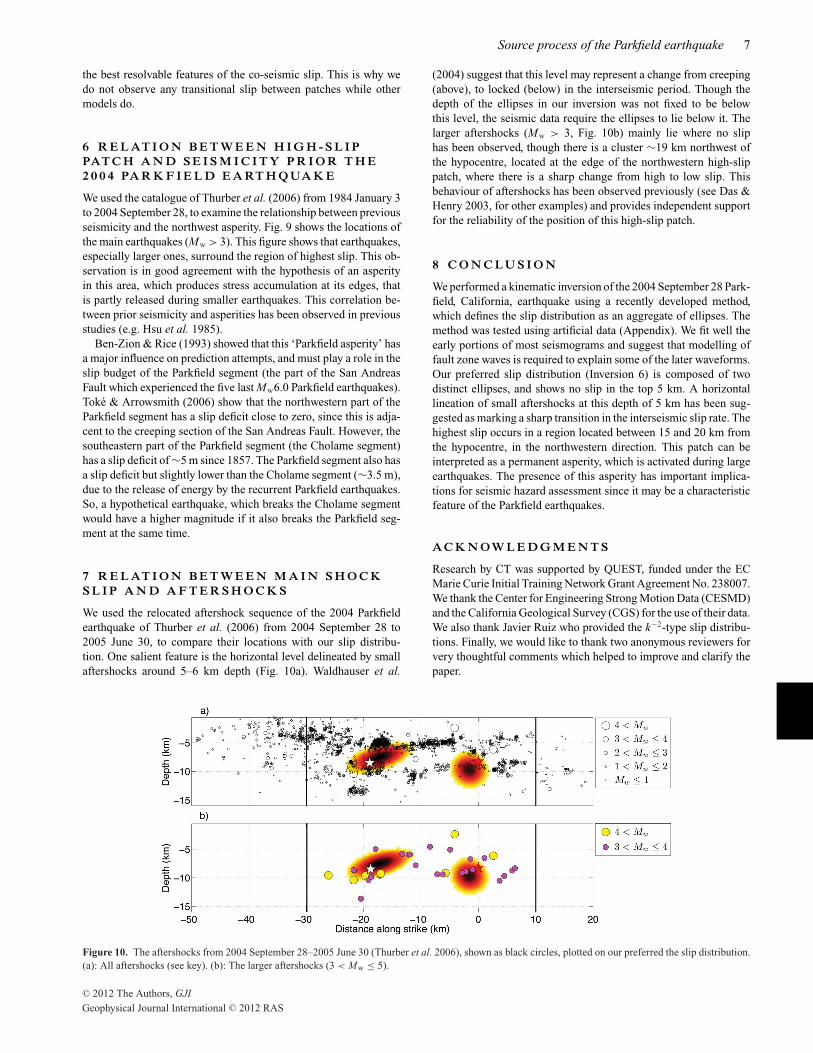
We used the relocated aftershock sequence of the 2004 Parkfieldearthquake of Thurber et al. (2006) from 2004 September 28 to2005 June 30, to compare their locations with our slip distribu-tion. One salient feature is the horizontal level delineated by smallaftershocks around 5–6 km depth (Fig. 10a). Waldhauser et al.

(2004) suggest that this level may represent a change from creeping(above), to locked (below) in the interseismic period. Though thedepth of the ellipses in our inversion was not fixed to be belowthis level, the seismic data require the ellipses to lie below it. Thelarger aftershocks (Mw > 3, Fig. 10b) mainly lie where no sliphas been observed, though there is a cluster ∼19 km northwest ofthe hypocentre, located at the edge of the northwestern high-slippatch, where there is a sharp change from high to low slip. Thisbehaviour of aftershocks has been observed previously (see Das &Henry 2003, for other examples) and provides independent supportfor the reliability of the position of this high-slip patch.

8 C O N C LU S I O N

We performed a kinematic inversion of the 2004 September 28 Park-field, California, earthquake using a recently developed method,which defines the slip distribution as an aggregate of ellipses. Themethod was tested using artificial data (Appendix). We fit well theearly portions of most seismograms and suggest that modelling offault zone waves is required to explain some of the later waveforms.Our preferred slip distribution (Inversion 6) is composed of twodistinct ellipses, and shows no slip in the top 5 km. A horizontallineation of small aftershocks at this depth of 5 km has been sug-gested as marking a sharp transition in the interseismic slip rate. Thehighest slip occurs in a region located between 15 and 20 km fromthe hypocentre, in the northwestern direction. This patch can beinterpreted as a permanent asperity, which is activated during largeearthquakes. The presence of this asperity has important implica-tions for seismic hazard assessment since it may be a characteristicfeature of the Parkfield earthquakes.

A C K N OW L E D G M E N T S

Research by CT was supported by QUEST, funded under the ECMarie Curie Initial Training Network Grant Agreement No. 238007.We thank the Center for Engineering Strong Motion Data (CESMD)and the California Geological Survey (CGS) for the use of their data.We also thank Javier Ruiz who provided the k−2-type slip distribu-tions. Finally, we would like to thank two anonymous reviewers forvery thoughtful comments which helped to improve and clarify thepaper.

Figure 10. The aftershocks from 2004 September 28–2005 June 30 (Thurber et al. 2006), shown as black circles, plotted on our preferred the slip distribution.(a): All aftershocks (see key). (b): The larger aftershocks (3 < Mw ≤ 5).




R E F E R E N C E S

Allmann, B.P. & Shearer, P.M., 2007. A high-frequency secondary eventduring the 2004 Parkfield earthquake, Science, 318, 1279–1283.

Bakun, W.H. & Lindh, A.G., 1985. The Parkfield, California, earthquakeprediction experiment, Science, 229, 619–624.

Bakun, W.H. & McEvilly, T.V., 1979. Earthquakes near Parkfield, California:comparing the 1934 and 1966 sequences, Science, 205, 1375–1377.

Ben-Zion, Y., 1998. Properties of seismic fault zone waves and their utilityfor imaging low-velocity structures, J. geophys. Res., 103, 12 567–12 585.

Ben-Zion, Y. & Rice, J.R., 1993. Earthquake failure sequences along acellular fault zone in a three-dimensional elastic solid containing asperityand nonasperity regions, J. geophys. Res., 98, 14 109–14 131.

Borcherdt, R.D. et al., 1985. A general earthquake observation system(geos), Bull. seism. Soc. Am., 75, 1783–1825.

Borcherdt, R.D., Johnston, M.J.S., Glassmoyer, G. & Dietel, C., 2006.Recordings of the 2004 Parkfield earthquake on the General EarthquakeObservation System Array: implications for earthquake precursors, faultrupture, and coseismic strain change, Bull. seism. Soc. Am., 96, 73–89.

Bouchon, M., 1981. A simple method to calculate Green’s functions forelastic layered media, Bull. seism. Soc. Am., 71, 959–971.

Cotton, F. & Coutant, O., 1997. Dynamic stress variations due to shear faultsin a plane-layered medium, Geophys. J. Int., 128, 676–688.

Custodio, S. & Archuleta, R.J., 2007. Parkfield earthquakes: char-acteristic or complementary? J. geophys. Res., 112, B05310,doi:10.1029/2006JB004617.

Custodio, S., Page, M.T. & Archuleta, R.J., 2009. Constraining earth-quake source inversion with GPS data: 2. A two-step approach to com-bine seismic and geodetic data sets, J. geophys. Res., 114, B01315,doi:10.1029/2008JB005746.

Das, S. & Henry, C., 2003. Spatial relation between main earth-quake slip and its aftershock distribution, Rev. Geophys., 41(3), 1013,doi:10.1029/2002RG000119.

Das, S. & Kostrov, B.V., 1990. Inversion for seismic slip rate and distributionwith stabilizing constraints: application to the 1986 Andrean of Islandsearthquake, J. geophys. Res., 95, 6899–6913.

Das, S. & Kostrov, B.V., 1994. Diversity of solution of the problem ofearthquake faulting inversion: application to SH waves for the great 1989Macquarie Ridge earthquake, Phys. Earth planet. Inter., 85, 293–318.

Di Carli, S., Francois-Holden, C., Peyrat, S. & Madariaga, R., 2010.Dynamic inversion of the 2000 Tottori earthquake based on el-liptical subfault approximations, J. geophys. Res., 115, B12238,doi:10.1029/2009JB006358.

Fletcher, J.B., Spudich, P. & Baker, L.M., 2006. Rupture propagation of the2004 Parkfield, California, earthquake from observation at the UPSAR,Bull. seism. Soc. Am., 96, 129–142.

Fukushima, K., Kanaori, Y. & Miura, F., 2010. Influence of fault processzone on ground shaking of inland earthquakes: verification of Mj=7.3Western Tottori Prefecture and Mj=7.0 West Off Fukuoka Prefectureearthquakes, southwest Japan, Eng. Geo., 116, 157–165.

Harris, R.A. & Segall, P., 1987. Detection of a locked zone at depth on theParkfield, California, segment of the San Andreas Fault, J. geophys. Res.,92, 7945–7962.

Hsu, V., Helsley, C.E., Berg, E. & Novelo-Casanova, D.A., 1985. Correlationof foreshocks and aftershocks and asperities, 122, 878–893.

Johanson, I.A., Fielding, E.J., Rolandone, F. & Burgmann, R., 2006. Coseis-mic and postseismic slip of the 2004 Parkfield earthquake from space-geodetic data, Bull. seism. Soc. Am., 96, S269–S282.

Johnson, K.M., Burgmann, R. & Larson, K., 2006. Frictional properties onthe San Andreas Fault near Parkfield, California, inferred from modelson afterslip following the 2004 earthquake, Bull. seism. Soc. Am., 96,S321–S338.

Kennett, B.L.N. & Kerry, N.J., 1979. Seismic waves in a stratified half space,Geophys. J. R. astr. Soc., 57, 557–583.

Li, Y.G., Leary, P., Aki, K. & Malin, P., 1990. Seismic trapped modes in theOroville and San Andreas Fault zones, Science, 249, 763–766.

Li, Y.G., Vidale, J.E. & Cochran, E.S., 2004. Low-velocity damaged struc-ture of the San Andreas Fault at Parkfield from fault zone trapped waves,Geophys. Res. Lett., 31, L12S06, doi:10.1029/2003GL019044.

Liu, P., Custodio, S. & Archuleta, R.J., 2006. Kinematic inversion of the 2004Mw6.0 Parkfield earthquake including an approximation to site effects,Bull. seism. Soc. Am., 96, 143–158.

Liu, P., Custodio, S. & Archuleta, R.J., 2008. Erratum to kinematic inversionof the 2004 Mw6.0 Parkfield earthquake including an approximation tosite effects, Bull. seism. Soc. Am., 98, 2101–2010.

Ma, S., Custodio, S., Archuleta, R.J. & Liu, P., 2008. Dynamic modeling ofthe 2004 Mw6.0 Parkfield, California earthquake, J. geophys. Res., 113,B02301, doi:10.1029/2007JB005216.

Malin, P.E., Blakeslee, S.N., Alvarez, M.G. & Martin, A.J., 1989. Mi-croearthquake imaging of the Parkfield asperity, Science, 244, 557–559.

Murray, J. & Langbein, J., 2006. Slip on the San Andreas fault at Parkfield,California, over two earthquake cycles and the implications for seismichazard, Bull. seism. Soc. Am., 96, 283–303.

Peyrat, S., Madariaga, R., Buforn, E., Campos, J., Asch, G. & Vilotte, J.P.,2010. Kinematic rupture process of the 2007 Tocopila earthquake and itsmain aftershocks from teleseismic and strong-motion data, Geophys. J.Int., 182, 1411–1430.

Ruiz, J.A., Baumont, D., Bernard, P. & Berge-Thierry, C., 2007. New ap-proach in the kinematic k−2 source model for generating physical slipvelocity functions, Geophys. J. Int., 171, 739–754.

Sambridge, M., 1999a. Geophysical inversion with a neighbourhoodalgorithm—I. Searching a parameter space, Geophys. J. Int., 138,479–494.

Sambridge, M., 1999b. Geophysical inversion with a neighbourhoodalgorithm—II. Appraising the ensemble, Geophys. J. Int., 138, 727–746.

Shakal, A., Haddadi, H., Graizer, V., Lin, K. & Huang, M., 2006. Some keyfeatures of the Strong Motion data from the M6.0 Parkfield, California,earthquake of 28 September 2004, Bull. seism. Soc. Am., 96, S90–S118.

Smith, B.R. & Sandwell, D.T., 2006. A model of the earthquake cycle alongthe San Andreas fault system for the past 1000 years, J. geophys. Res.,111, B01405, doi:10.1029/2005JB003703.

Spudich, P. & Miller, D.P., 1990. Seismic site effects and the spatial interpo-lation of earthquake seismograms: results using aftershocks of the 1986North Palm Springs, California, earthquake, Bull. seism. Soc. Am., 80,1504–1532.

Thurber, C., Zhang, H., Waldhauser, F., Hardebeck, J., Michael, A. &Eberhart-Phillips, D., 2006. Three-dimensional compressional wavespeedmodel, earthquake relocations, and focal mechnisms for the Parkfield,California, region, Bull. seism. Soc. Am., 96, 38–49.

Toke, N.A. & Arrowsmith, J.R., 2006. Reassessment of a slip budget alongthe Parkfield segment of the San Andreas Fault, Bull. seism. Soc. Am., 96,S339–S348.

Toppozada, T.R., Branum, D.M., Reichle, M.S. & Hallstrom, C.L., 2002.San Andreas fault zone, California: M ≤ 5.5 earthquake history, Bull.seism. Soc. Am., 92, 2555–2601.

Trifunac, M.D., 1974. A three-dimensional dislocation model for the SanFernando, California, earthquake of February 9, 1971, Bull. seism. Soc.Am., 64, 149–172.

Vallee, M. & Bouchon, M., 2004. Imaging coseismic rupture in far field byslip patches, Geophys. J. Int., 156, 615–630.

Voronoi, M.G., 1908. Nouvelles applications des parametres continus a latheorie des formes quadratiques, J. reine Angew. Math., 134, 198–287.

Waldhauser, F., Ellsworth, W.L., Shaff, D.P. & Cole, A., 2004. Streaks, mul-tiplets, and holes: high-resolution spatio-temporal behavior of Parkfieldseismicity, Geophys. Res. Lett., 31, L18608, doi:10.1029/2004GL020649.

A P P E N D I X A : T E S T O F T H EI N V E R S I O N M E T H O D, U S I N GA RT I F I C I A L DATA

We construct artificial data, using the same configuration as pre-sented in the main paper, for the digital stations. The rupture isinitiated at the same location than the 2004 Parkfield earthquakehypocentre, rupturing with a prescribed rupture velocity of 3 km s−1.Three tests, using three different slip distributions, were carried out.The rupture velocity and the moment of the artificial earthquake isretrieved almost perfectly for each of the tests.




For this earthquake, we have used results from previous studies tochoose the number of ellipses to use. However, if we want to applythis method blindly, some tests on how to choose the number ofellipses need to be carried out. This will be considered in ‘Test 3’.

A1 Test 1

Artificial displacement seismograms were generated at digital sta-tion locations for a model with two distinct ellipses. This test wascarried out to see how the programmes performed in a very simplecase. Fig. A1 shows the artificial model (a) and the inverted model(b). The artificial model is almost perfectly retrieved. The majordifference is seen in the amplitude of the ellipses, with the rightside ellipse being 7 per cent higher than the initial model and theleft ellipse being 13 per cent lower. The fit to the data is very good(ε = 0.03), and there is no difference between the artificial data andthe solution seismograms.

Figure A1. ‘Test 1’—(a) Artificial slip distribution used to generate thesynthetic seismograms. (b) Inverted slip distribution.

A2 Test 2

The artificial seismograms were generated for a k−2-type slip dis-tribution (Fig. A2a), following the method described in Ruiz et al.(2007). In the inversion, we allow rupture and slip to occur only ona single asperity located near the hypocentre. The result is shown

Figure A2. ‘Test 2’—Same as Fig. A1 with the blue line in (a) being the0.7 m slip contour.

Figure A3. Comparison of the solution seismograms (red) with the artificialdata (blue) for ‘Test 2’.

in Fig. A2(b). The blue line on Fig. A2(a) shows the contour ofthe ellipse inferred from the inversion. We can see that the mainasperity of the artificial model and the ellipse of the inversion arespatially close, though the ellipse is bigger than the main asperity.This is because the inversion is constrained to include all the slipof the artificial model within a single patch, while it aims to obtainthe proper moment and fit the seismograms. This test shows thatdespite the heterogeneous slip distribution of the artificial model,the inversion method retrieves the main asperity. The seismogramsshow a good fit (ε = 0.16), with small mismatch at some stations(Fig. A3). This can be explained by the small amplitude asperities,which we do not try to extract.

A3 Test 3

This test is performed using a k−2-type, double asperity, slip dis-tribution. One goal here is to gain insight into how to choose the

Figure A4. ‘Test 3’ (one ellipse): same as Fig. A2.




Figure A5. ‘Test 3’: same as Fig. A3.

number of ellipses to be used in the inversion, when no other stud-ies of an earthquake exists. It was suggested by Vallee & Bouchon(2004) that the number of ellipses should be increased when partof the signal, believed to be caused by source, is not fitted, a pro-cedure that they applied to the 1995 Jalisco (Mexico) earthquake.To explicitly illustrate this, we first invert the artificial model usingonly one ellipse. The slip distribution obtained from the inversionand the comparison of the waveforms are shown in Figs A4 and A5,respectively. We can see that in the case where two major asperitiesare present, the inversion tends to produce a final slip distributionwith an ellipse located at the centroid of the distribution. However,examination of the displacement waveforms shows non-negligiblemismatch between the solution seismograms and the artificial ones(ε = 0.19). In a real problem, this would have alerted us to thefact that a higher number of ellipses are needed. We next usedtwo ellipses to see if the fit is improved. The results are shownin Fig. A6 (comparison of final slip distribution). The two-ellipseinversion correctly retrieves the two major asperities. The inverted

Figure A6. ‘Test 3’ (two ellipses): same as Fig. A2.

model also shows a small patch with high amplitude between thetwo ellipses. This does coincides with a small peak in amplitude inthe artificial model, but is more likely an artefact of the inversiondue to the proximity of the two ellipses. The waveform fits are alsosignificantly improved (ε = 0.05).

S U P P O RT I N G I N F O R M AT I O N

Additional Supporting Information may be found in the online ver-sion of this article:

Table S1. Details of the different inversions carried out in this studyand the resulting source processes.Supplementary Information S2 (Section S1–S15). Comparisonbetween the observed and solution seismograms for the two differentsets of stations (digital and analogue). Labels at the top of eachpage give the name of the Inversion as described in the main text.A summary of the parameters describing each Inversion is alsoattached with this file.

Please note: Wiley-Blackwell are not responsible for the content orfunctionality of any supporting materials supplied by the authors.Any queries (other than missing material) should be directed to thecorresponding author for the article.



Documents

Geophysical Journal International - UMR 8538madariag/Papers/Twardzik_Parkf.pdf · Geophysical Journal International Geophys. J. Int. (2012) doi: 10.1111/j.1365-246X.2012.05653.x GJI