W phase source inversion for moderate to large …wphase.unistra.fr/zacharie/papers/DuputelEtal2012a.pdfGeophys. J. Int. (2012) doi: 10.1111/j.1365-246X.2012.05419.x GJI Seismology

Geophys. J. Int. (2012) doi: 10.1111/j.1365-246X.2012.05419.x

GJI

Sei

smol

ogy

W phase source inversion for moderate to large earthquakes(1990–2010)

Zacharie Duputel,1 Luis Rivera,2 Hiroo Kanamori1 and Gavin Hayes3

1Seismological Laboratory, California Institute of Technology, Pasadena, CA, USA. E-mail: [email protected] de Physique du Globe de Strasbourg, IPGS - UMR 7516, CNRS and Universite de Strasbourg (EOST), France3U.S. Geological Survey, National Earthquake Information Center (contracted by Synergetics, Inc.), Golden, CO, USA

Accepted 2012 February 10. Received 2012 February 10; in original form 2011 February 6

S U M M A R YRapid characterization of the earthquake source and of its effects is a growing field of interest.Until recently, it still took several hours to determine the first-order attributes of a greatearthquake (e.g. Mw ! 7.5), even in a well-instrumented region. The main limiting factorswere data saturation, the interference of different phases and the time duration and spatialextent of the source rupture. To accelerate centroid moment tensor (CMT) determinations, wehave developed a source inversion algorithm based on modelling of the W phase, a very longperiod phase (100–1000 s) arriving at the same time as the P wave. The purpose of this work isto finely tune and validate the algorithm for large-to-moderate-sized earthquakes using threecomponents of W phase ground motion at teleseismic distances. To that end, the point sourceparameters of all Mw ! 6.5 earthquakes that occurred between 1990 and 2010 (815 events)are determined using Federation of Digital Seismograph Networks, Global SeismographicNetwork broad-band stations and STS1 global virtual networks of the Incorporated ResearchInstitutions for Seismology Data Management Center. For each event, a preliminary magnitudeobtained from W phase amplitudes is used to estimate the initial moment rate function halfduration and to define the corner frequencies of the passband filter that will be applied to thewaveforms. Starting from these initial parameters, the seismic moment tensor is calculatedusing a preliminary location as a first approximation of the centroid. A full CMT inversionis then conducted for centroid timing and location determination. Comparisons with Harvardand Global CMT solutions highlight the robustness of W phase CMT solutions at teleseismicdistances. The differences in Mw rarely exceed 0.2 and the source mechanisms are very similarto one another. Difficulties arise when a target earthquake is shortly (e.g. within 10 hr) precededby another large earthquake, which disturbs the waveforms of the target event. To deal withsuch difficult situations, we remove the perturbation caused by earlier disturbing events bysubtracting the corresponding synthetics from the data. The CMT parameters for the disturbedevent can then be retrieved using the residual seismograms. We also explore the feasibilityof obtaining source parameters of smaller earthquakes in the range 6.0 " Mw < 6.5. Resultssuggest that the W phase inversion can be implemented reliably for the majority of earthquakesof Mw = 6 or larger.

Key words: Tsunamis; Earthquake source observations; Surface waves and free oscillations;Wave propagation; Early warning.

1 I N T RO D U C T I O N

Considerable effort has been made over the last two decades regard-ing the design and implementation of tools aimed at fast characteri-zation of earthquake sources. Magnitudes, moment tensors, rupturepatterns, shake maps, tsunami excitation and propagation scenariosare now routinely calculated and disseminated by several agencieswhenever a significant earthquake occurs. The interest in making

these estimations quickly available is twofold. Authorities and reliefagencies can use them to plan and perform rescue and aid opera-tions. Earth scientists, on the other hand, rely upon this informationto make critical decisions on re-programming a satellite orbit, ordesigning a field experiment, etc. The delay in availability of suchresults is highly variable and depends on the size of the event, itslocation on the globe and on the type of required result itself. Forexample, for an Mw = 5 earthquake occurring today in Japan or in

C# 2012 The Authors 1Geophysical Journal International C# 2012 RAS

Geophysical Journal International

zac

Typewritten Text

(reprint)

2 Z. Duputel et al.

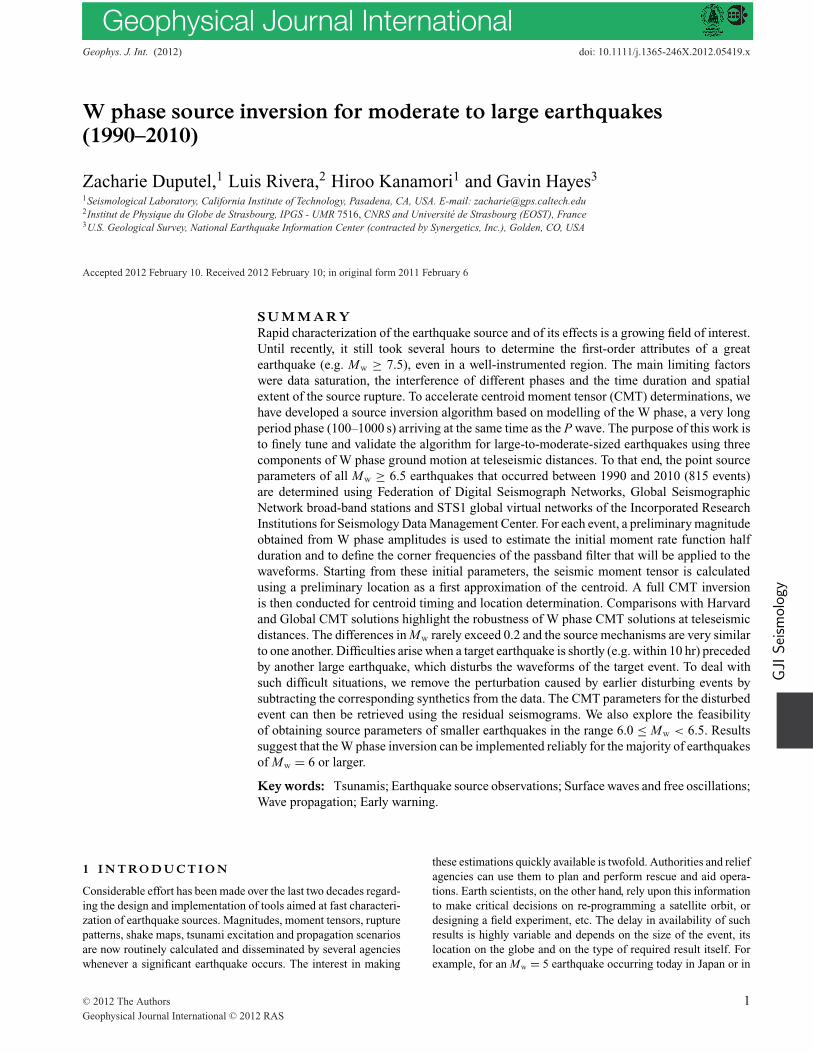
Figure 1. W phase source inversion results for the 2004 great Sumatra–Andaman Islands earthquake. W phase CMT (WCMT) and Global CMT (GCMT)solutions are shown in the topleft corner. Examples of observed waveforms (black lines) and the corresponding synthetics (red lines) computed from theWCMT solution are presented. The station azimuth (!) and epicentral distance (") are indicated as well as W phase time window, which are bounded by reddots. The WCMT inversion is based on the ground motion of stations within " " 90$ after applying a bandpass filter in the 1–5 mHz passband. W phase andlater arrivals are often very well predicted by the WCMT solution although many channels have instrument problems during or after the surface waves arrivals(most of the broad-band data within " " 40$ are saturated).

California, a fairly reliable magnitude estimation is available withina few minutes after the origin time. As an opposite end-member,it usually takes at least several hours before a reliable slip distri-bution is determined for a large earthquake (Mw > 7.0) even in awell-instrumented region (e.g. Hayes et al. 2011).

Although it is desirable to reduce such a delay, there are severelimitations in this practice. The rupture process of large events canlast several minutes, and any analyses based on the beginning of therecords can only provide a lower bound to the magnitude estimate orto the extent of the associated rupture. Although it is always possibleto use some hypothetical, simplified model to predict the final mag-nitude from signals generated during the early stages of the rupture,there is increasing evidence for a wide diversity in the nature ofseismic sources (Kanamori 2004), which translates into significantvariations in narrow-band magnitude estimations. In addition to therupture duration, it is also necessary to account for wave propaga-tion time, which can be substantial (e.g. 9 min for a direct P wavefrom a shallow event to be recorded at " = 50$). The use of nearbyor regional records would then appear as desirable. Unfortunately,we do not always have good regional coverage with the existingglobal networks. Even in cases where regional data are available,the use of seismological records close to the source (say " < 5$) canbe problematic because such data are more sensitive to variations

in the shallow structure of the Earth. Their use therefore requiresan accurate earth model which incorporates 3-D regional hetero-geneity (Tsuruoka et al. 2009). Furthermore, if the rupture lengthis large, a point source approximation can be problematic for theclosest stations even when analysing long periods. Finally, regionaland even teleseismic records of large events are often saturatedacross the frequency range. For example, most of the broad-banddata available at the Federation of Digital Seismograph Network(FDSN) stations within 40$ of the 2004 Sumatra–Andaman Islandsearthquake rupture are saturated at the arrival time of the surfacewaves. (Fig. 1).

To overcome these limitations, we have developed a centroid mo-ment tensor (CMT) inversion algorithm using the W phase, a verylong period phase (100–1000 s) identified after the 1992 Nicaraguatsunami earthquake by Kanamori (1993). Use of the W phase forfast and accurate quantification of the source properties of greatearthquakes is advantageous for several reasons. First, the W phasehas a fast group velocity, which facilitates rapid inversion after anearthquake occurs. Second, the major part of the propagating energyassociated with the W phase is confined to the mantle, which is lessheterogeneous than the crust, thus resulting in a relatively simplewaveform. Finally, the W phase has a very long period character,which is essential for the source inversion of large earthquakes.

C# 2012 The Authors, GJIGeophysical Journal International C# 2012 RAS

W phase inversion for Mw ! 6.0 earthquakes 3

Table 1. Number of events as a function of date and magnitude.

6.50–6.74 6.75–6.99 7.00–7.24 7.25–7.49 7.50–7.99 8.00–9.00 Total

1990–1993 65 39 25 7 11 0 1471994–1997 72 40 32 5 17 3 1691998–2001 53 35 23 10 13 3 1372002–2005 72 26 19 14 11 4 1462006–2009 71 40 15 17 17 5 1652010–2010 18 14 6 9 3 1 51

Total 351 194 120 62 72 16 815

In general, long periods increasingly dominate the wavefield asmoment grows because the duration of rupture gets longer as theevent gets larger. Furthermore, the size of the ruptured fault andthe amount of final slip control the tsunami wave height. The long-period wavefield is also useful for the source analysis of tsunamiearthquakes, defined by Kanamori (1972). These events are of-ten characterized by an anomalously long-period spectrum at thesource, which produces unusually large tsunami height relative toshort-period magnitude estimations ("100 s, e.g. M s). In the spe-cific case of CMT determinations, it is also fundamental to considervery long period waves since the point source approximation is usedeven for earthquakes rupturing large faults (!100 km).

The W phase CMT algorithm was initially developed byKanamori & Rivera (2008) using the inversion of vertical com-ponents of ground motion. For brevity, we will refer to this paperas KR. A real-time application at the National Earthquake Informa-tion Center (NEIC) using this version of the algorithm was set upby Hayes et al. (2009) for Mw ! 5.8 earthquakes on a global scale.The algorithm has now been extended to all three components ofthe ground motion and has been deployed in real time at the Institutde Physique du Globe de Strasbourg (IPGS) for testing purposes, atNEIC and at the Pacific Tsunami Warning Center (PTWC) of theNational Oceanic and Atmospheric Administration (Duputel et al.2011). We have also adapted the inversion for use on the regionalscale, an application which is currently being tested in California,Japan, Mexico and Taiwan (Rivera & Kanamori 2009; Rivera et al.2010).

The purpose of this work is to fine-tune and validate the W phasealgorithm for large to moderate earthquakes using three-componentground motions at regional and teleseismic distances. To this end,the point source parameters of all Mw ! 6.5 earthquakes that oc-curred between 1990 and 2010 (815 events) are systematically de-termined using FDSN, Global Seismographic Network broad-bandstations (GSN_BROADBAND) and STS1 global virtual networks.Although our new W phase catalogue is complete to Mw = 6.5, wealso explore the use of the W phase inversion for all earthquakes be-tween 6.0 " Mw < 6.5, to assess whether reliable source parameterscan also be obtained for smaller events.

In subsequent sections, we focus on the application of the Wphase inversion to produce a complete catalogue of events for allMw ! 6.5 earthquakes since 1990. Although the approach used forsmaller events is the same, we discuss this specific application ina separate section, as the resulting W phase catalogue is no longercomplete and as such should be distinguished from our main focus.

2 DATA A N D P R E L I M I NA RYT R E AT M E N T S

We use three-component broad-band data of moderate to large earth-quakes that occurred in the period 1990–2010 and were recorded atregional and teleseismic distances. To have a homogeneous refer-

ence catalogue, we start from the Global CMT (GCMT; Dziewonski1982; Ekstrom et al. 2005; Ekstrom & Nettles 2006) database andselect all the events with Mw ! 6.5. We use the moment tensorelements provided by GCMT to compute scalar moment M0 usingSilver & Jordan (1982)’s and Dahlen & Tromp (1998)’s definitionof M0 =%!

i j Mi j Mi j /2 and Mw as

Mw = 23

(log10(M0) & 16.10) (1)

with M0 in dyne-cm (Kanamori 1977; Hanks & Kanamori 1979).Table 1 lists the magnitude distribution of these events as a functionof time.

Our main criterion for data selection is the availability of a broad-band sensor. Four types of sensor dominate our data set: STS-1,STS-2, KS-5400 and CMG-3T. Data are obtained through NetDCfrom the data holdings at the Incorporated Research Institutions forSeismology Data Management Center (IRIS DMC) and Geoscope.We use 1 s-sampled data (LHZ) mostly from II, IU, G, GE andMN networks. Some additional stations from other FDSN-affiliatednetworks are also included to improve spatial coverage. For somestations, several streams are available (different location-IDs). Insuch cases, we give priority to the longer period sensor. Coverageis quite variable, and depends not only on the event size and itsepicentral location, but also on time as a result of the improvementof the worldwide broad-band station distribution since 1990 (Fig. 2).

To design the W phase source inversion, we have to choose theproper time window and passband corner frequencies. FollowingKR, at a given epicentral distance ", the W phase time win-dow extends from the theoretical P arrival time tP(") to tP(") +15 s deg&1 ' ". The end time is chosen here to ensure that thetime window ends before the arrival of large surface wave trains.The original standard frequency band used in KR for large events(Mw ! 8.0) was 1–5 mHz. However, to have a sufficiently highsignal-to-noise ratio for smaller events, it is necessary to graduallyshift the passband towards higher frequencies (Hayes et al. 2009,see Table 2). This is related to the well-known behaviour of thebackground noise steadily growing at periods longer than 200 s.The long-period edge of the bandpass filter is also dictated by thefact that some of the seismometers used become noisy at very longperiods. To choose the appropriate bandpass corner frequencies(Table 2) prior to the inversion of each event, we perform a pre-liminary magnitude estimation by measuring the overall verti-cal W phase amplitude in the 1–5 mHz bandpass as detailed inSection 3.3.

Following KR, both instrumental deconvolution (to ground dis-placement) and bandpass filtering (fourth order, causal, Butter-worth) are implemented in the time domain as infinite impulseresponse (IIR) filters. Working in the time domain is very usefulfor real-time operations since the data can be processed sampleby sample as they become available. Moreover, in contrast to tradi-tional frequency-domain deconvolution, it allows the retrieval of the


4 Z. Duputel et al.

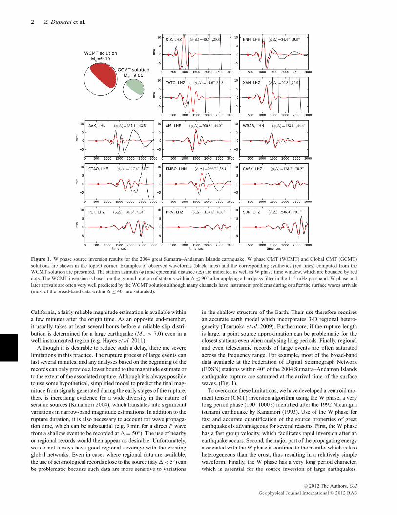
Figure 2. Data coverage for LH channels extracted from SEED volumes of Mw ! 6.5 events for virtual networks: FDSN, GSN_BROADBAND and STS1between 1990 and 2010. The number of LH channels is shown in (a) whereas the azimuthal coverage is presented in (b). The total number of available LHchannels is shown in black. For stations within epicentral distance " " 90$, the selected W phase traces before and after the data screening are presented,respectively, in red and blue.

Table 2. Corner frequencies used for butterworthbandpass filtering (fourth order, causal) in Wphase inversion when using three components. Thefrequency passbands used by Hayes et al. (2009)were defined for W phase inversion using onlyvertical components.

Magnitude range Passband filter, mHz (s)

Mw-wprel ! 8.0 1.0–5.0 (200–1000)8.0 > Mw-wprel ! 7.5 1.7–6.7 (150–500)7.5 > Mw-wprel ! 7.0 2.0–8.3 (120–500)7.0 > Mw-wprel ! 6.5 4.0–10.0 (100–250)

W phase on records clipped at the arrival of large-amplitude surfacewaves. Once cut to length, traces are concatenated to build the dataset to be used in the inversion.

Finally, two data sets are defined for each event according tothe maximal epicentral distance: 5$ < " < 50$ and 5$ < " <

90$. The first data set is available 22 min after the origin time; thesecond requires an additional 13 min. The reason for using thesetwo distinct data sets will be made clear in the next section.

3 M E T H O D O L O G Y

3.1 Overall real-time operation protocol

The W phase centroid moment tensor (WCMT) inversion is ina way similar to the approach of Dziewonski et al. (1981) andDziewonski & Woodhouse (1983). The three main differences are(1) the time window, (2) the longer periods used in the WCMTinversion and (3) the algorithm employed to determine the best pointsource location (centroid). The source parameters to be determinedare the elements of the seismic moment tensor f = [Mrr, M ## , M!! ,Mr# , Mr! , M #!]t and the four space–time coordinates of the centroid!c = [#c, !c, rc, $c]t where # c is the colatitude, !c is the longitude,rc is the radius and $ c is the centroid time. The full WCMT solution

vector can thus be defined as

m ="

f!c

#. (2)

Here, we use the term ‘centroid’ following the common practicein source inversion studies, but what we actually determine is thebest point source location and the mechanism. Thus, the centroidlocation and CMT here should be interpreted as the best point sourcelocation and the moment tensor, respectively. The centroid !c canbe estimated by seeking the point source location that minimizes aquadratic misfit function between the W phase data vector (dw) andthe corresponding synthetic vector (sw)

% (m) = 12

(sw(m) & dw)·(sw(m) & dw). (3)

The synthetic seismograms sw are obtained from pre-computedGreen’s functions calculated using normal mode summation foran epicentral distance range of 0$ " " " 90$ with an interval of0.1$ and for a depth range of 0–760 km. These Green’s functions arecomputed using the Preliminary Reference Earth Model (PREM)from Dziewonski & Anderson (1981). The effect of finite-sourceduration on W phase traces is accounted for by assuming the mo-ment rate function (MRF) to be an isosceles triangle of half durationhc centred at $ c. There are two main reasons why the location andorigin time estimated from body wave arrivals cannot be assumed asthe centroid. First, the errors in hypocentral parameters can be sub-stantial when they are obtained within minutes of the origin time.Secondly, for large earthquakes the hypocentre can be significantlydifferent from the centroid.

Fig. 3 presents the overall algorithm we follow in this study.The horizontal axis represents increasing time and does not includeeffects of data latency. Let us then suppose that somewhere on theglobe an event occurs at t = t0 and at ta ( t0 + 10 min or so, wereceive from some agency the preliminary epicentral coordinates,depth and origin time. For brevity, we will call this information thepreliminary determination of epicentre (PDE). In the context of this



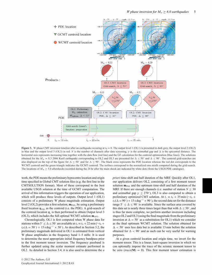
Figure 3. W phase CMT inversion timeline after an earthquake occuring at t0 = 0. The output level 1 (OL1) is presented in dark grey, the output level 2 (OL2)in blue and the output level 3 (OL3) in red. N is the number of channels after data screening, & is the azimuthal gap and " is the epicentral distance. Thehorizontal axis represents increasing time together with the data flow (red line) and the GF calculation for the centroid optimization (blue lines). The solutionsobtained for the Mw = 8.3 2006 Kuril earthquake corresponding to OL2 and OL3 are presented for " " 50$ and " " 90$. The centroid grid-searches arealso displayed on the top of the figure for " " 50$ and for " " 90$. The black cross represents the PDE location whereas the red dot corresponds to theWCMT centroid and the green triangle indicates the GCMT centroid. The isolines correspond to the normalized rms misfit computed during the grid-search.The locations of Mw ! 5.0 aftershocks recorded during the 24 hr after the main shock are indicated by white dots (from the USGS PDE catalogue).

work, the PDE means the preliminary hypocentre location and origintime specified in Global CMT solution files (e.g. the first line in theCMTSOLUTION format). Most of these correspond to the bestavailable USGS solution at the time of GCMT computation. Thearrival of this information triggers the operation of our application,which will produce three levels of outputs. Output level 1 (OL1)consists of a preliminary W phase magnitude estimation. Outputlevel 2 (OL2) provides a first solution, mPDE, by using a preliminaryfixed location !PDE as the centroid (i.e. the PDE). A grid-search ofthe centroid location !c is then performed to obtain Output level 3(OL3), which includes the full optimal WCMT solution mOPT.

Chronologically, OL1 is first computed when W phase data forstations within 5$ " " " 50$ are available at tb ) t0 + 22 min ((t0 +tP(" = 50$) + 15 s deg&1 ' 50$). As described in Section 3.2, thepreliminary magnitude delivered in OL1 is estimated from verticalW phase amplitudes in the frequency band 1–5 mHz. It is usedto determine the most appropriate initial frequency bandpass priorto the first moment tensor inversion. The frequency passband isfurther updated using the scalar moment estimate performed inOL2. As detailed in Section 3.4, it is also used to determine the a

priori time-shift and half duration of the MRF. Quickly after OL1,our application delivers OL2, consisting of a first moment tensorsolution mPDE and the optimum time-shift and half duration of theMRF. If there are enough channels (i.e. number of station N ! 30and azimuthal gap & " 270$), OL3 is also computed to obtain apreliminary optimized CMT solution. At tc ) t0 + 35 min ((t0 +tP(" = 90$) + 15 s deg&1 ' 90$), the second data set for the distancerange 5$ " " " 90$ is available. Since the surface area covered bythis data set is nearly three times larger than that with " " 50$, andis thus far more complete, we perform another inversion includingstages OL2 and OL3 (using the final magnitude from the preliminaryinversion at " = 50$ as a substitution for OL1) which we consideras the final optimum WCMT solution. The solution obtained for" < 50$ uses less data but is available 13 min before the solutionobtained for " < 90$ and as such can be very useful for warningpurposes.

At a given centroid location and origin time, we invert for themoment tensor. This is a linear, least-square inversion in which wecan optionally impose the trace of the seismic moment tensor tobe zero (trace(M) = 0). This first moment tensor estimation is


6 Z. Duputel et al.

quasi-instantaneous. Only when thousands of synthetic seismo-grams are calculated does the computation time become significant.This is the case for OL3, where we want to perform an inversion foreach potential location !c on a 3-D grid surrounding the epicentre!PDE. Despite the computation-time cost, we prefer this approach tothose based on local derivatives of eq. (3) (as in Dziewonski et al.1981; Dziewonski & Woodhouse 1983), because of its robustnessin a radially varying earth. In real-time operations, the computationdelay can be reduced by computing Green’s functions over a gridgeometry defined around the initial PDE received at time ta. Sincethis computation takes place as the W phase is travelling to thestations, by the time the W phase data are available at tb and tc, allthe Green’s functions are ready to be used in the inversions.

In practice, for this study where we are dealing with past events,the data are made available to the application instantaneously asevent SEED volumes containing both the seismic traces and theinstrumental responses.

3.2 Data screening

An important task throughout the inversion process is data screen-ing. Both in real time and for further analysis, we need to handlesituations in which some bad traces are included in the data set(e.g. noisy or dead channels, bad instrument responses, incompletetraces, etc.). As described in the next paragraphs, screening filtersare set up at different stages of the WCMT algorithm to identifyand remove such records.

Following KR, we fit the instrumental response of each sensorwithin a pre-defined frequency band (0.001–100 Hz) to that of a sim-ple electromagnetic velocimeter with three free parameters: naturalperiod, viscous damping and gain factor. If the result of this fit isgood enough (misfit smaller than 3 per cent) the response is storedin a look-up table in the form of the coefficients of the recursivefilter to be used for deconvolution; otherwise, the correspondingtraces are discarded. In general, the volume of rejected data at thisstage is extremely small.

The first screening performed is a ‘noise screening’, which isused to reject the noisiest traces. The pre-event displacement powerspectral densities (PSDs) are computed for the whole data set usinga duration of 3 hr preceding the origin time. We reject any channelfor which the average difference between its noise curve and theNew High Noise Model (NHNM; Peterson 1993) in the frequencyband 1–10 mHz is positive (i.e. very noisy traces).

Any incomplete trace over the interval [tP, tP + 15 s deg&1 ' "]is also removed from the data set. Although in some cases it could betechnically feasible to use such a trace (thanks to the time-domainanalysis we use), we prefer not to use them to maintain a simplealgorithm and to avoid potential data artefacts.

Next, a ‘median screening’ is used to reject traces associated withincorrect instrument responses and to remove glitchy or dead chan-nels. It is applied after performing the time-domain deconvolutionand bandpass filtering, according to the following procedure. Foreach trace j, we compute its peak-to-peak value pj in the W phasetime window. From the complete set of pj, we compute the event’smedian value m, and reject traces with pj significantly different fromm (pi < 0.1 ' m or pi > 3 ' m). Although this screening methodcan accidentally reject some good data (e.g. a nodal station), ithas the advantage of being completely independent of the misfit ineq. (3) and does not require any forward modelling.

Finally, we apply a ‘misfit screening’ based on the similaritybetween observed and synthetic W phase traces. After performing

a WCMT inversion, we can compute the rms misfit according to

'i = *siw & di

w*2

*sw*2, (4)

where siw and di

w are, respectively, the synthetic and data traces cor-responding to the ith channel. The normalization is used to dampenthe effect of the event’s magnitude. ' i is then compared with a giventhreshold 'max. Those stations for which ' i > 'max are removed be-fore restarting a new inversion with the reduced data set. Severalthresholds corresponding to increasingly more stringent criteria aresuccessively applied. In the present application, we use three con-secutive thresholds: 'max = 3.0, 'max = 2.0 and 'max = 1.0.

Fig. 2 presents the fraction of LH channels that remain afterapplying these data screening filters. The initial number of filesextracted from SEED volumes is presented in black, the number ofchannels selected for " " 90$ is shown in red and the final numberof W traces after the screening processes is presented in blue. Onaverage for Mw ! 6.5 earthquakes occuring between 1990 and2010, 50 per cent of channels are rejected during the data screeningprocess.

In this work, we define ‘disturbed events’ as any earthquakewhose signal is contaminated by the large amplitude waveforms ofa preceding event. More precisely, they are defined as events occur-ring within 1 hr of Mw ! 6.5 events, or less than 10 hr after Mw

! 7.0 earthquakes, and which demonstrate a poor station distribu-tion after the data screening process for " " 50$ (i.e. N < 30 or& > 270$). The standard W phase algorithm is not well suited tomodel such events because the assumption of an isolated source intime and space is no longer valid. Using this approach, 44 disturbedearthquakes have been recognized and rejected from our catalogue.The list of ‘disturbed event’ over the period 1990–2010 is detailedin Table S1. In Section 4.5, we explore a possible scheme to handlethem in real time.

3.3 Preliminary W phase magnitude estimation (OL1)

At tb = t0 + tP(" = 50$) + 15 s deg&1 ' 50$ ( t0 + 22 min, W phasetraces for all stations within " < 50$ are available and the first dataset can be built. Before trying a formal inversion for the momenttensor, we perform a first-order fit of the W phase amplitudes as afunction of distance and azimuth. Following KR, the idea here is tocapture the information carried by the overall vertical amplitude ofW phase and to translate it into magnitude.

After instrument correction of vertical component data and band-pass filtering in the 1-5 mHz range, we remove incomplete tracesand apply a ‘median screening’ to remove conspicuous outliers. Wethen measure the peak-to-peak value pj on each W trace j. Theseamplitudes are then reduced to a common distance (" = 40$).This procedure is similar to the Richter Magnitude original defi-nition (Richter 1935). To capture the overall amplitude level whileallowing some azimuthal variations due to the mechanism, thesereduced amplitudes are matched to a two-lobe azimuthal patterncorresponding to a pure thrust or normal-fault earthquake

p j = q(" j )[a & b cos2(( j & (0)], (5)

where q("j) is the W phase amplitude decay (see Table 2 of KR)and a, b and (0 the parameters to be determined. Eq. (5) can besolved as a linear least-square problem by inverting for a & b/2 (theaverage amplitude), b cos (2(0)/2 and b sin (2(0)/2. The resultingaverage amplitude a & b/2 can then be used as a direct measure ofthe seismic moment. It is also useful to solve for (0 if we want to



obtain a rough estimate of the fault strike !. This choice of a two-lobe azimuthal pattern associated with a pure thrust mechanismis motivated by the fact that the W phase algorithm is primarilytargeted at the inversion of large tsunamigenic earthquakes.

The purpose of this preliminary estimation is twofold. First, itprovides a quick, simple and robust magnitude estimation which isindependent of any additional hypothesis and modelling details; thisis the first output, OL1, of our algorithm. Secondly, the magnitudeso obtained can be used as a proxy for the initial estimate of theduration of the moment rate function to be used in subsequent stages.Note that neither the focal mechanism nor the centroid depth areneeded for this preliminary magnitude estimation.

3.4 MT inversion at PDE (OL2)

After performing the ‘noise screening’, rejecting channels show-ing a bad instrumental response fit or with truncated records andapplying a ‘median screening’, we perform a first moment tensorinversion. As is typical in moment tensor inversion algorithms, weimpose a zero trace to the moment tensor to cope with the poorresolution of the isotropic components for shallow earthquakes(Mendiguren 1977). It constrains the seismic source to have nonet volume change.

Besides the waveforms, we need a centroid location, centroidtime and an MRF duration. At tb ( t0 + 22 min, we use the PDElocation as our best guess for the centroid location, whereas theduration is estimated by a scaling law from the seismic momentobtained in OL1

hc = 1.2 ' 10&8 ' M1/30 , (6)

where hc is in seconds and M0 in dyne-cm. This relation is obtainedfrom the constant stress drop scaling relation hc + M1/3

0 (Kanamori& Anderson 1975). The constant of proportionality is set so that anearthquake with M0 = 1027dyne-cm (Mw = 7.3) has a half durationof 12s. At tc ( t0 + 35 min, we use the duration obtained at OL2for " " 50$.

We can then select the corresponding Green’s functions from thedatabase, convolve them with the MRF shape and apply the samebandpass filter as applied to the data.

One more parameter is necessary to compute synthetic tracesdirectly comparable to the waveform data: the delay $ c betweenorigin time (i.e. PDE) and the centroid time. This is determinedwith a grid-search by performing several moment tensor inversionsfor a range of trial values of $ c. This is an inexpensive opera-tion since changing this delay requires simply a time-shift of theGreen’s functions or of the data traces in the opposite direction.As a result of this grid-search, we obtain an optimal delay value.In contrast to $ c, the MRF duration hc is poorly constrained bythe waveforms, being generally significantly smaller than the longperiods of the W phase. We thus use the optimal delay value asa new proxy for hc (i.e. we assume that hc = $ c). With these pa-rameters, we compute three successive moment tensor inversionsusing an increasingly stringent ‘misfit screening’ with thresholds'max = 3.0, 'max = 2.0 and 'max = 1.0 for the channel rms misfitin eq. (4). The resulting moment tensor solution is our second-leveloutput, OL2.

3.5 Optimized CMT inversion (OL3)

After determining the optimum centroid time and MRF half du-ration, we attempt to find a centroid location which is better thanthe preliminary location estimate. For this purpose, we set up a3-D grid-search (latitude–longitude-depth), where each grid-nodeis used as a potential centroid location and a complete WCMT in-version is made. The rms misfit in eq. (3) is used as an objectivefunction to choose the optimal centroid location. To make certainthat the rms values for different centroids are comparable, we mustuse the same data set. For this reason, we do not apply any additionalscreening at this level. The typical dimension of the grid is 2.4$ '2.4$ ' 100 km, centred on the PDE location, and the minimum al-lowed centroid depth is 12 km. The depth step ("h) is variable withthe centroid depth (h)

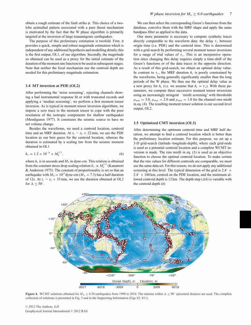
Figure 4. WCMT solutions obtained for Mw ! 6.50 earthquakes from 1990 to 2010. The stations within " " 90$ epicentral distance are used. The completecollection of solutions is presented in Fig. 5 and in the Supporting Information (Figs S2–S11).


8 Z. Duputel et al.

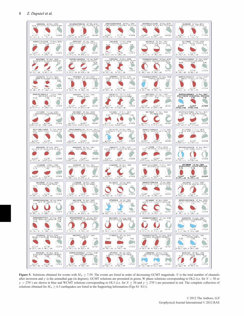
Figure 5. Solutions obtained for events with Mw ! 7.59. The events are listed in order of decreasing GCMT magnitude. N is the total number of channelsafter inversion and & is the azimuthal gap (in degrees). GCMT solutions are presented in green, W phase solutions corresponding to OL2 (i.e. for N < 30 or& > 270$) are shown in blue and WCMT solutions corresponding to OL3 (i.e. for N ! 30 and & " 270$) are presented in red. The complete collection ofsolutions obtained for Mw ! 6.5 earthquakes are listed in the Supporting Information (Figs S1–S11).



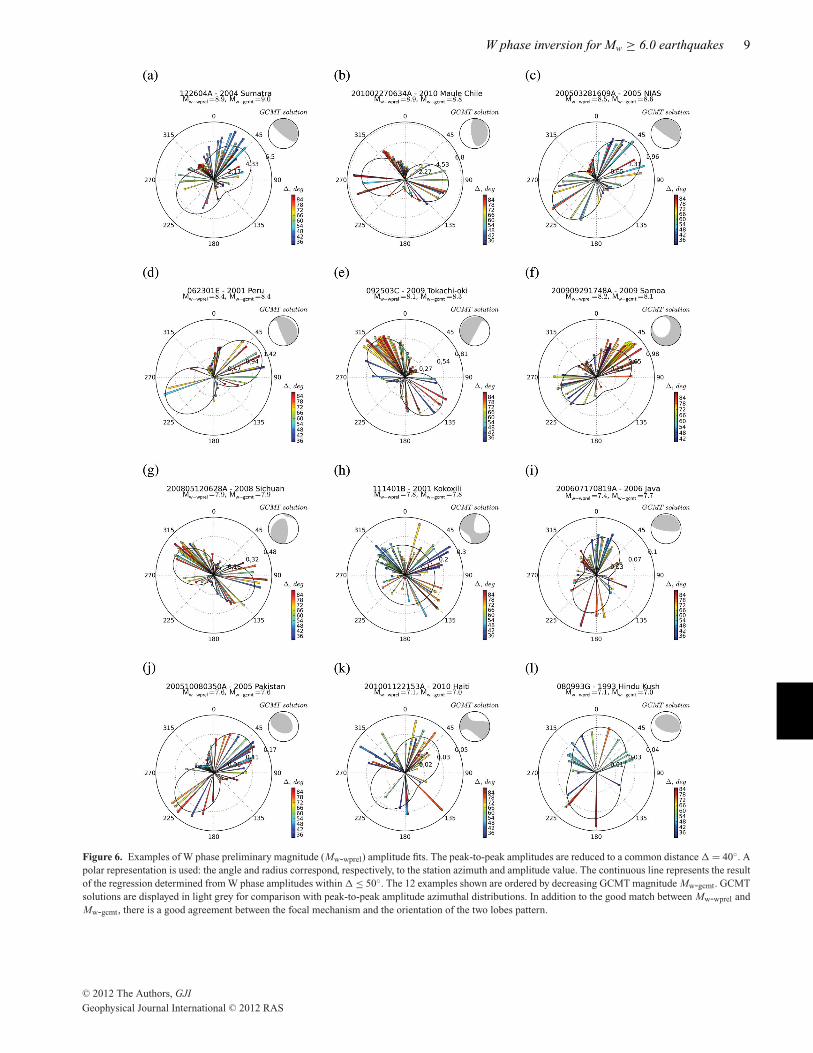
Figure 6. Examples of W phase preliminary magnitude (Mw-wprel) amplitude fits. The peak-to-peak amplitudes are reduced to a common distance " = 40$. Apolar representation is used: the angle and radius correspond, respectively, to the station azimuth and amplitude value. The continuous line represents the resultof the regression determined from W phase amplitudes within " " 50$. The 12 examples shown are ordered by decreasing GCMT magnitude Mw-gcmt. GCMTsolutions are displayed in light grey for comparison with peak-to-peak amplitude azimuthal distributions. In addition to the good match between Mw-wprel andMw-gcmt, there is a good agreement between the focal mechanism and the orientation of the two lobes pattern.


10 Z. Duputel et al.

(1) "h = 2 km for h " 25.5,(2) "h = 5 km for 25.5 " h " 50.5,(3) "h = 10 km for h ! 50.5.

A multiple-scale grid-search is performed for each depth: First,a global exploration of the latitude–longitude space is conductedusing a large sampling step (40 km). We then select several locationswhich represent the best least-squares misfits between observedand calculated waveforms. Another exploration is then performedaround these optimal points by increasing the horizontal samplingresolution (10 km). The initial grid size is increased if one of thechosen locations is within one cell of the grid edge. Finally, wechoose the centroid depth, latitude and longitude which minimizethe rms misfit in eq. (3) and take them as the optimum WCMTcentroid (OL3).

4 R E S U LT S

In this section, we present the results of applying the protocol de-fined earlier to earthquakes with Mw ! 6.50 since 1990 (i.e. 815events), and systematically compare them with the GCMT solutions.Fig. 4 shows the global distribution of the WCMT mechanisms. InFig. 5, we present detailed solutions for Mw ! 7.59 events togetherwith GCMT solutions for comparison. In the online SupportingInformation, we provide WCMT and GCMT solutions for Mw !6.5 earthquakes (Figs S1–S11) and the solutions resulting from theextension to 6.0 " Mw < 6.5 events (Figs S13–S36). Solutions forMw ! 6.5 earthquakes using data within " < 90$ are also availableat: http://eost.u-strasbg.fr/wphase/MGE65.

4.1 Preliminary magnitude estimation

In Fig. 6, 12 examples of distance-corrected amplitude–azimuthfits are presented. In each panel, the continuous line represents theregression whereas the coloured bars indicate the corrected peak-to-peak values at different epicentral distances. The fits are generallygood, even for stations at large epicentral distances (" > 50$),

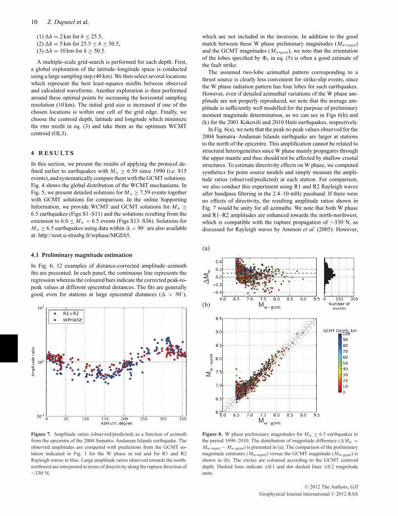
Figure 7. Amplitude ratios (observed/predicted) as a function of azimuthfrom the epicentre of the 2004 Sumatra–Andaman Islands earthquake. Theobserved amplitudes are compared with predictions from the GCMT so-lution indicated in Fig. 1 for the W phase in red and for R1 and R2Rayleigh waves in blue. Large amplitude ratios observed towards the north-northwest are interpreted in terms of directivity along the rupture direction of(330$N.

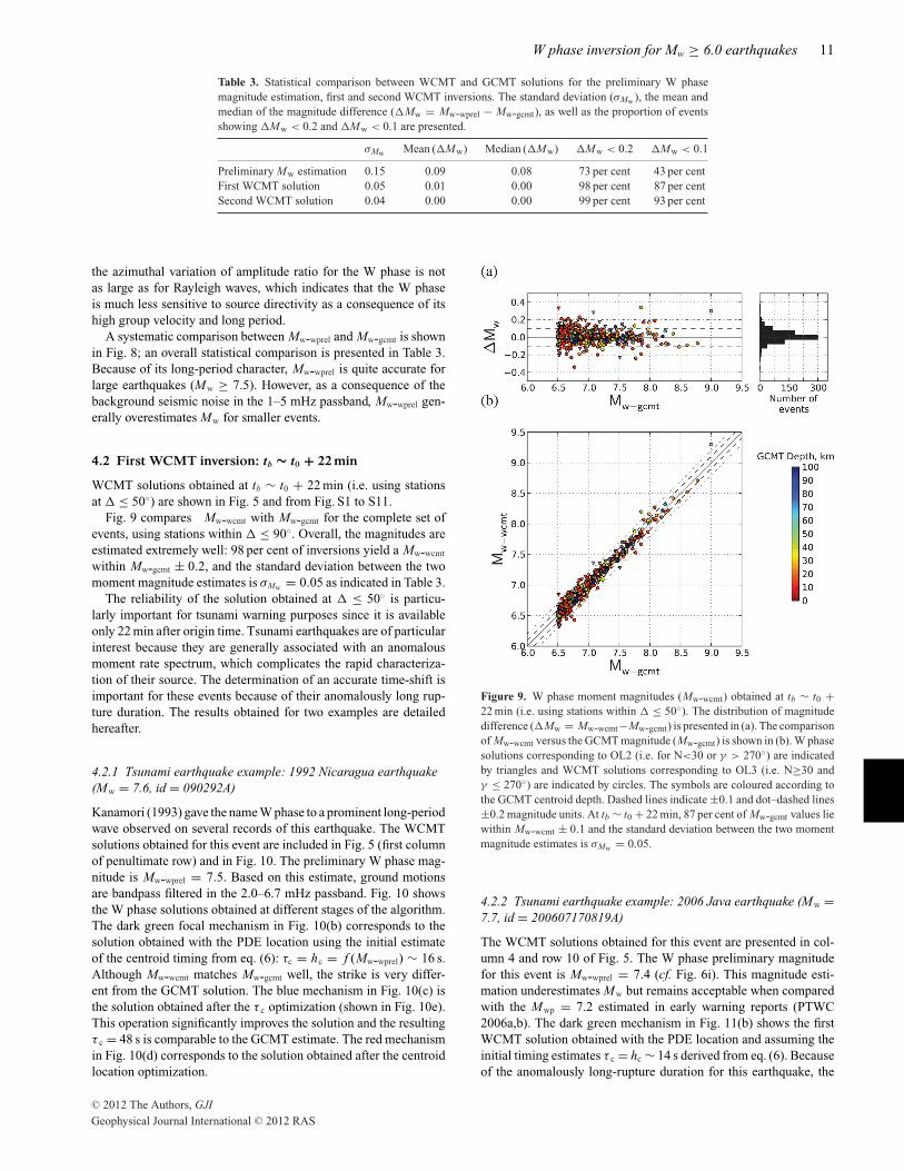
which are not included in the inversion. In addition to the goodmatch between these W phase preliminary magnitudes (Mw-wprel)and the GCMT magnitudes (Mw-gcmt), we note that the orientationof the lobes specified by (0 in eq. (5) is often a good estimate ofthe fault strike.

The assumed two-lobe azimuthal pattern corresponding to athrust source is clearly less convenient for strike-slip events, sincethe W phase radiation pattern has four lobes for such earthquakes.However, even if detailed azimuthal variations of the W phase am-plitude are not properly reproduced, we note that the average am-plitude is sufficiently well modelled for the purpose of preliminarymoment magnitude determination, as we can see in Figs 6(h) and(k) for the 2001 Kokoxili and 2010 Haiti earthquakes, respectively.

In Fig. 6(a), we note that the peak-to-peak values observed for the2004 Sumatra–Andaman Islands earthquake are larger at stationsto the north of the epicentre. This amplification cannot be related tostructural heterogeneities since W phase mainly propagates throughthe upper mantle and thus should not be affected by shallow crustalstructures. To estimate directivity effects on W phase, we computedsynthetics for point source models and simply measure the ampli-tude ratios (observed/predicted) at each station. For comparison,we also conduct this experiment using R1 and R2 Rayleigh wavesafter bandpass filtering in the 2.4–10 mHz passband. If there wereno effects of directivity, the resulting amplitude ratios shown inFig. 7 would be unity for all azimuths. We note that both W phaseand R1–R2 amplitudes are enhanced towards the north-northwest,which is compatible with the rupture propagation of (330$N, asdiscussed for Rayleigh waves by Ammon et al. (2005). However,

Figure 8. W phase preliminary magnitudes for Mw ! 6.5 earthquakes inthe period 1990–2010. The distribution of magnitude difference ("Mw =Mw-wprel & Mw-gcmt) is presented in (a). The comparison of the preliminarymagnitude estimates (Mw-wprel) versus the GCMT magnitude (Mw-gcmt) isshown in (b). The circles are coloured according to the GCMT centroiddepth. Dashed lines indicate ±0.1 and dot–dashed lines ±0.2 magnitudeunits.



Table 3. Statistical comparison between WCMT and GCMT solutions for the preliminary W phasemagnitude estimation, first and second WCMT inversions. The standard deviation ()Mw ), the mean andmedian of the magnitude difference ("Mw = Mw-wprel & Mw-gcmt), as well as the proportion of eventsshowing "Mw < 0.2 and "Mw < 0.1 are presented.

)Mw Mean ("Mw) Median ("Mw) "Mw < 0.2 "Mw < 0.1

Preliminary Mw estimation 0.15 0.09 0.08 73 per cent 43 per centFirst WCMT solution 0.05 0.01 0.00 98 per cent 87 per centSecond WCMT solution 0.04 0.00 0.00 99 per cent 93 per cent

the azimuthal variation of amplitude ratio for the W phase is notas large as for Rayleigh waves, which indicates that the W phaseis much less sensitive to source directivity as a consequence of itshigh group velocity and long period.

A systematic comparison between Mw-wprel and Mw-gcmt is shownin Fig. 8; an overall statistical comparison is presented in Table 3.Because of its long-period character, Mw-wprel is quite accurate forlarge earthquakes (Mw ! 7.5). However, as a consequence of thebackground seismic noise in the 1–5 mHz passband, Mw-wprel gen-erally overestimates Mw for smaller events.

4.2 First WCMT inversion: tb ! t0 + 22 min

WCMT solutions obtained at tb ( t0 + 22 min (i.e. using stationsat " " 50$) are shown in Fig. 5 and from Fig. S1 to S11.

Fig. 9 compares Mw-wcmt with Mw-gcmt for the complete set ofevents, using stations within " " 90$. Overall, the magnitudes areestimated extremely well: 98 per cent of inversions yield a Mw-wcmt

within Mw-gcmt ± 0.2, and the standard deviation between the twomoment magnitude estimates is )Mw = 0.05 as indicated in Table 3.

The reliability of the solution obtained at " " 50$ is particu-larly important for tsunami warning purposes since it is availableonly 22 min after origin time. Tsunami earthquakes are of particularinterest because they are generally associated with an anomalousmoment rate spectrum, which complicates the rapid characteriza-tion of their source. The determination of an accurate time-shift isimportant for these events because of their anomalously long rup-ture duration. The results obtained for two examples are detailedhereafter.

4.2.1 Tsunami earthquake example: 1992 Nicaragua earthquake(Mw = 7.6, id = 090292A)

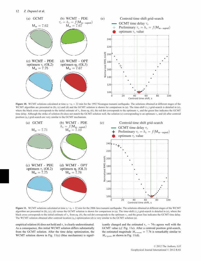
Kanamori (1993) gave the name W phase to a prominent long-periodwave observed on several records of this earthquake. The WCMTsolutions obtained for this event are included in Fig. 5 (first columnof penultimate row) and in Fig. 10. The preliminary W phase mag-nitude is Mw-wprel = 7.5. Based on this estimate, ground motionsare bandpass filtered in the 2.0–6.7 mHz passband. Fig. 10 showsthe W phase solutions obtained at different stages of the algorithm.The dark green focal mechanism in Fig. 10(b) corresponds to thesolution obtained with the PDE location using the initial estimateof the centroid timing from eq. (6): $c = hc = f (Mw-wprel) ( 16 s.Although Mw-wcmt matches Mw-gcmt well, the strike is very differ-ent from the GCMT solution. The blue mechanism in Fig. 10(c) isthe solution obtained after the $ c optimization (shown in Fig. 10e).This operation significantly improves the solution and the resulting$ c = 48 s is comparable to the GCMT estimate. The red mechanismin Fig. 10(d) corresponds to the solution obtained after the centroidlocation optimization.

Figure 9. W phase moment magnitudes (Mw-wcmt) obtained at tb ( t0 +22 min (i.e. using stations within " " 50$). The distribution of magnitudedifference ("Mw = Mw-wcmt&Mw-gcmt) is presented in (a). The comparisonof Mw-wcmt versus the GCMT magnitude (Mw-gcmt) is shown in (b). W phasesolutions corresponding to OL2 (i.e. for N<30 or & > 270$) are indicatedby triangles and WCMT solutions corresponding to OL3 (i.e. N!30 and& " 270$) are indicated by circles. The symbols are coloured according tothe GCMT centroid depth. Dashed lines indicate ±0.1 and dot–dashed lines±0.2 magnitude units. At tb ( t0 + 22 min, 87 per cent of Mw-gcmt values liewithin Mw-wcmt ± 0.1 and the standard deviation between the two momentmagnitude estimates is )Mw = 0.05.

4.2.2 Tsunami earthquake example: 2006 Java earthquake (Mw =7.7, id = 200607170819A)

The WCMT solutions obtained for this event are presented in col-umn 4 and row 10 of Fig. 5. The W phase preliminary magnitudefor this event is Mw-wprel = 7.4 (cf. Fig. 6i). This magnitude esti-mation underestimates Mw but remains acceptable when comparedwith the Mwp = 7.2 estimated in early warning reports (PTWC2006a,b). The dark green mechanism in Fig. 11(b) shows the firstWCMT solution obtained with the PDE location and assuming theinitial timing estimates $ c = hc ( 14 s derived from eq. (6). Becauseof the anomalously long-rupture duration for this earthquake, the



Figure 10. WCMT solutions calculated at time tb(t0 + 22 min for the 1992 Nicaragua tsunami earthquake. The solutions obtained at different stages of theWCMT algorithm are presented in (b), (c) and (d) and the GCMT solution is shown for comparison in (a). The time-shift ($ c) grid-search is detailed in (e),where the black cross corresponds to the initial estimate of $ c from eq. (6), the red dot corresponds to the optimum $ c and the green line indicates the GCMTtime delay. Although the strike of solution (b) does not match the GCMT solution well, the solution (c) corresponding to an optimum $ c and (d) after centroidposition (*c) grid-search are very similar to the GCMT mechanism.

Figure 11. WCMT solutions calculated at time tb(t0 + 22 min for the 2006 Java tsunami earthquake. The solutions obtained at different stages of the WCMTalgorithm are presented in (b), (c), (d) versus the GCMT solution is shown for comparison in (a). The time-shift ($ c) grid-search is detailed in (e), where theblack cross corresponds to the initial estimate of $ c from eq. (6), the red dot corresponds to the optimum $ c and the green line indicates the GCMT time delay.The WCMT solution obtained after centroid location (*c) optimization (d) is very similar to the GCMT solution (a).

empirical relation (6) does not hold and $ c is clearly underestimated.As a consequence, this initial WCMT solution differs substantiallyfrom the GCMT solution. After the time delay optimization, theWCMT solution shown in Fig. 11(c) (blue mechanism) is signif-

icantly changed and the estimated $ c ( 74 s agrees well with theGCMT value (cf. Fig. 11e). After a centroid position grid-search,the estimated magnitude Mw-wcmt = 7.76 is remarkably similar toMw-gcmt, as shown in Fig. 11(d).



4.3 Second WCMT inversion: tc ! t0 + 35 min

The WCMT solutions obtained at tc ( t0 + 35 min (i.e. usingstations up to " " 90$) correspond to the mechanisms shown inthe middle of each frame in Fig. 5, and from Figs S1–S11. Thecomplete collection of solutions is also available at: http://eost.u-strasbg.fr/wphase/MGE65.

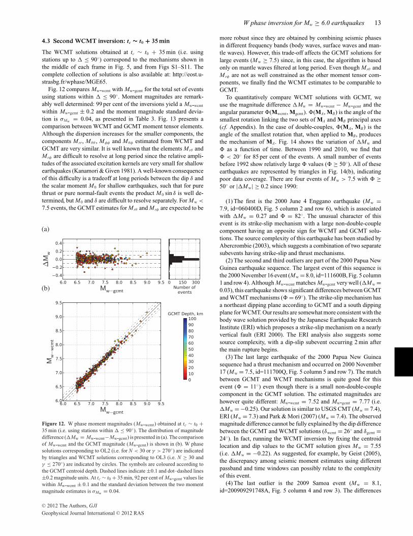
Fig. 12 compares Mw-wcmt with Mw-gcmt for the total set of eventsusing stations within " " 90$. Moment magnitudes are remark-ably well determined: 99 per cent of the inversions yield a Mw-wcmt

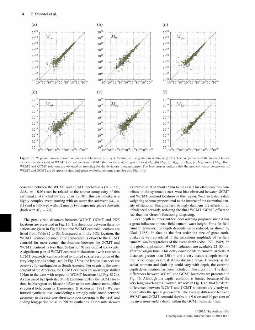
within Mw-gcmt ± 0.2 and the moment magnitude standard devia-tion is )Mw = 0.04, as presented in Table 3. Fig. 13 presents acomparison between WCMT and GCMT moment tensor elements.Although the dispersion increases for the smaller components, thecomponents Mrr, M ## , M!! and M #! estimated from WCMT andGCMT are very similar. It is well known that the elements Mr# andMr! are difficult to resolve at long period since the relative ampli-tudes of the associated excitation kernels are very small for shallowearthquakes (Kanamori & Given 1981). A well-known consequenceof this difficulty is a tradeoff at long periods between the dip + andthe scalar moment M0 for shallow earthquakes, such that for purethrust or pure normal-fault events the product M0 sin + is well de-termined, but M0 and + are difficult to resolve separately. For Mw <

7.5 events, the GCMT estimates for Mr# and Mr! are expected to be

Figure 12. W phase moment magnitudes (Mw-wcmt) obtained at tc ( t0 +35 min (i.e. using stations within " " 90$). The distribution of magnitudedifference ("Mw = Mw-wcmt&Mw-gcmt) is presented in (a). The comparisonof Mw-wcmt and the GCMT magnitude (Mw-gcmt) is shown in (b). W phasesolutions corresponding to OL2 (i.e. for N < 30 or & > 270$) are indicatedby triangles and WCMT solutions corresponding to OL3 (i.e. N ! 30 and& " 270$) are indicated by circles. The symbols are coloured according tothe GCMT centroid depth. Dashed lines indicate ±0.1 and dot–dashed lines±0.2 magnitude units. At tc ( t0 + 35 min, 92 per cent of Mw-gcmt values liewithin Mw-wcmt ± 0.1 and the standard deviation between the two momentmagnitude estimates is )Mw = 0.04.

more robust since they are obtained by combining seismic phasesin different frequency bands (body waves, surface waves and man-tle waves). However, this trade-off affects the GCMT solutions forlarge events (Mw ! 7.5) since, in this case, the algorithm is basedonly on mantle waves filtered at long period. Even though Mr# andMr! are not as well constrained as the other moment tensor com-ponents, we finally find the WCMT estimates to be comparable toGCMT.

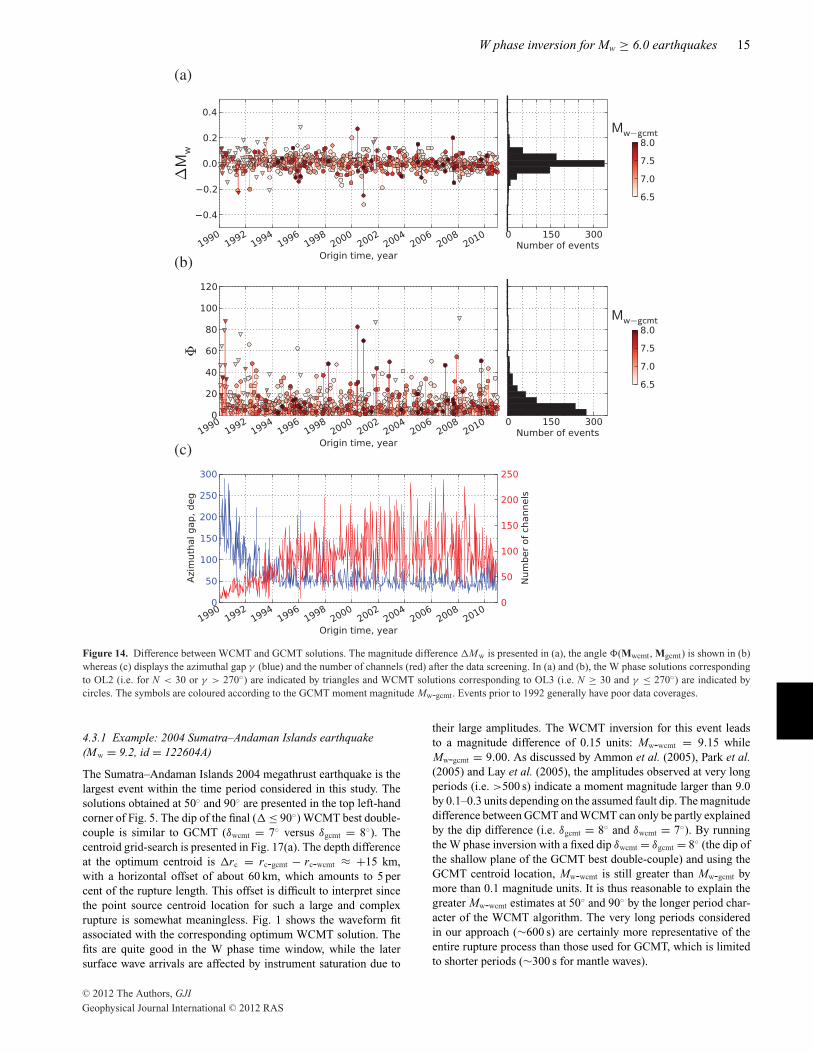
To quantitatively compare WCMT solutions with GCMT, weuse the magnitude difference "Mw = Mw-wcmt & Mw-gcmt and theangular parameter ((Mwcmt, Mgcmt). ((MA, MB) is the angle of thesmallest rotation linking the two sets of MA and MB principal axes(cf. Appendix). In the case of double-couples, ((MA, MB) is theangle of the smallest rotation that, when applied to MB, producesthe mechanism of MA. Fig. 14 shows the variation of "Mw and( as a function of time. Between 1990 and 2010, we find that( < 20$ for 85 per cent of the events. A small number of eventsbefore 1992 show relatively large ( values (( ! 50$). All of theseearthquakes are represented by triangles in Fig. 14(b), indicatingpoor data coverage. There are four events of Mw > 7.5 with ( !50$ or |"Mw| ! 0.2 since 1990:

(1) The first is the 2000 June 4 Enggano earthquake (Mw =7.9, id=060400D, Fig. 5 column 2 and row 6), which is associatedwith "Mw = 0.27 and ( = 82$. The unusual character of thisevent is its strike-slip mechanism with a large non-double-couplecomponent having an opposite sign for WCMT and GCMT solu-tions. The source complexity of this earthquake has been studied byAbercrombie (2003), which suggests a combination of two separatesubevents having strike-slip and thrust mechanisms.

(2) The second and third outliers are part of the 2000 Papua NewGuinea earthquake sequence. The largest event of this sequence isthe 2000 November 16 event (Mw = 8.0, id=111600B, Fig. 5 column1 and row 4). Although Mw-wcmt matches Mw-gcmt very well ("Mw =0.03), this earthquake shows significant differences between GCMTand WCMT mechanisms (( = 69$). The strike-slip mechanism hasa northeast dipping plane according to GCMT and a south dippingplane for WCMT. Our results are somewhat more consistent with thebody wave solution provided by the Japanese Earthquake ResearchInstitute (ERI) which proposes a strike-slip mechanism on a nearlyvertical fault (ERI 2000). The ERI analysis also suggests somesource complexity, with a dip-slip subevent occurring 2 min afterthe main rupture begins.

(3) The last large earthquake of the 2000 Papua New Guineasequence had a thrust mechanism and occurred on 2000 November17 (Mw = 7.5, id=111700Q, Fig. 5 column 5 and row 7). The matchbetween GCMT and WCMT mechanisms is quite good for thisevent (( = 11$) even though there is a small non-double-couplecomponent in the GCMT solution. The estimated magnitudes arehowever quite different: Mw-wcmt = 7.52 and Mw-gcmt = 7.77 (i.e."Mw = &0.25). Our solution is similar to USGS CMT (Mw = 7.4),ERI (Mw = 7.3) and Park & Mori (2007) (Mw = 7.4). The observedmagnitude difference cannot be fully explained by the dip differencebetween the GCMT and WCMT solutions (+wcmt = 26$ and +gcmt =24$). In fact, running the WCMT inversion by fixing the centroidlocation and dip values to the GCMT solution gives Mw = 7.55(i.e. "Mw = &0.22). As suggested, for example, by Geist (2005),the discrepancy among seismic moment estimates using differentpassband and time windows can possibly relate to the complexityof this event.

(4) The last outlier is the 2009 Samoa event (Mw = 8.1,id=200909291748A, Fig. 5 column 4 and row 3). The differences



Figure 13. W phase moment tensor components obtained at tc ( t0 + 35 min (i.e. using stations within " " 90$). The comparisons of the moment tensorelements (in dyne-cm) of WCMT (vertical axis) and GCMT (horizontal axis) are given for (a) Mrr, (b) M## , (c) M!! , (d) Mr# , (e) M#! and (f) M#! . BothWCMT and GCMT solutions are obtained by inverting for the deviatoric moment tensor. The blue crosses indicate that the moment tensor component ofWCMT and GCMT are of opposite sign, and green symbols, the same sign. See also Fig. 14(b).

observed between the WCMT and GCMT mechanisms (( = 51$,"Mw = &0.03) can be related to the source complexity of thisearthquake. As noted by Lay et al. (2010), this earthquake is ahighly complex event starting with an outer rise subevent (Mw =8.1) and is followed within 2 min by two major interplate subevents(both with Mw = 7.8).

The great-circle distances between WCMT, GCMT and PDElocations are presented in Fig. 15. The directions between these lo-cations are given in Fig. S12 and the WCMT centroid locations arelisted from Table S2 to S3. Compared with the PDE location, theWCMT location obtained after grid-search is closer to the GCMTcentroid for most events: the distance between the GCMT andWCMT centroid is less than 50 km for 91 per cent of the events.A significant part of WCMT centroid mislocations (with respect toGCMT centroids) can be related to limited spacial resolution of thevery long periods being used. In Fig. 15(b), the largest distances areobserved for earthquakes in South America. For events in the west-ern part of the Americas, the GCMT centroids are on average shifted30 km to the west with respect to WCMT locations (cf. Fig. S12b).As discussed by Hjorleifsdottir & Ekstrom (2010), the GCMT loca-tions in this region are biased (15 km to the west due to unmodelledstructural heterogeneity Dziewonski & Anderson (1981). We per-formed synthetic tests considering a strongly unbalanced networkgeometry in the east–west direction (poor coverage to the west) andadding long-period noise to PREM synthetics. Our results showed

a centroid shift of about 15 km to the east. This effect can thus con-tribute to the systematic east–west bias observed between GCMTand WCMT centroid locations in this region. We also tested a dataweighting scheme proportional to the inverse of the azimuthal den-sity of stations. This approach strongly dampens the effects of anunbalanced network, reducing the final WCMT–GCMT offsets toless than our Green’s function grid spacing.

Focal depth is important for local warning purposes since it hasa great influence on near-field tsunami wave height. For a far-fieldtsunami however, the depth dependence is reduced, as shown byOkal (1988). In fact, to the first order the size of great earth-quakes is well correlated to the maximum amplitude of far-fieldtsunami waves regardless of the event depth (Abe 1979, 1989). Inthis global application, WCMT solutions are available 22–35 minafter the origin time. This delay corresponds to tsunami arrivals atdistances greater than 250 km and a very accurate depth estima-tion is no longer essential at this distance range. However, as thescalar moment and fault dip could vary with depth, the centroiddepth determination has been included in the algorithm. The depthdifferences between WCMT and GCMT locations are presented inFig. 16. Although the depth resolution is limited because of thevery long wavelengths involved, we note in Fig. 16(c) that the depthdifferences between WCMT and GCMT solutions are clearly re-duced after the spatial grid-search. The average difference betweenWCMT and GCMT centroid depths is +9.6 km and 90 per cent ofthe inversions yield a depth within the GCMT value ±11 km.



Figure 14. Difference between WCMT and GCMT solutions. The magnitude difference "Mw is presented in (a), the angle ((Mwcmt, Mgcmt) is shown in (b)whereas (c) displays the azimuthal gap & (blue) and the number of channels (red) after the data screening. In (a) and (b), the W phase solutions correspondingto OL2 (i.e. for N < 30 or & > 270$) are indicated by triangles and WCMT solutions corresponding to OL3 (i.e. N ! 30 and & " 270$) are indicated bycircles. The symbols are coloured according to the GCMT moment magnitude Mw-gcmt. Events prior to 1992 generally have poor data coverages.

4.3.1 Example: 2004 Sumatra–Andaman Islands earthquake(Mw = 9.2, id = 122604A)

The Sumatra–Andaman Islands 2004 megathrust earthquake is thelargest event within the time period considered in this study. Thesolutions obtained at 50$ and 90$ are presented in the top left-handcorner of Fig. 5. The dip of the final (" " 90$) WCMT best double-couple is similar to GCMT (+wcmt = 7$ versus +gcmt = 8$). Thecentroid grid-search is presented in Fig. 17(a). The depth differenceat the optimum centroid is "rc = rc-gcmt & rc-wcmt , +15 km,with a horizontal offset of about 60 km, which amounts to 5 percent of the rupture length. This offset is difficult to interpret sincethe point source centroid location for such a large and complexrupture is somewhat meaningless. Fig. 1 shows the waveform fitassociated with the corresponding optimum WCMT solution. Thefits are quite good in the W phase time window, while the latersurface wave arrivals are affected by instrument saturation due to

their large amplitudes. The WCMT inversion for this event leadsto a magnitude difference of 0.15 units: Mw-wcmt = 9.15 whileMw-gcmt = 9.00. As discussed by Ammon et al. (2005), Park et al.(2005) and Lay et al. (2005), the amplitudes observed at very longperiods (i.e. >500 s) indicate a moment magnitude larger than 9.0by 0.1–0.3 units depending on the assumed fault dip. The magnitudedifference between GCMT and WCMT can only be partly explainedby the dip difference (i.e. +gcmt = 8$ and +wcmt = 7$). By runningthe W phase inversion with a fixed dip +wcmt = +gcmt = 8$ (the dip ofthe shallow plane of the GCMT best double-couple) and using theGCMT centroid location, Mw-wcmt is still greater than Mw-gcmt bymore than 0.1 magnitude units. It is thus reasonable to explain thegreater Mw-wcmt estimates at 50$ and 90$ by the longer period char-acter of the WCMT algorithm. The very long periods consideredin our approach ((600 s) are certainly more representative of theentire rupture process than those used for GCMT, which is limitedto shorter periods ((300 s for mantle waves).



Figure 15. Distances between WCMT, GCMT and PDE locations. The great-circle distance "xPDE between the PDE location and the GCMT centroid isshown on the map (a) and in the histogram with blue bars (c). The distance "xc between GCMT and WCMT centroid locations is presented in (b) and in thehistogram with red bars (c).

Figure 16. Depth difference between GCMT and WCMT locations before and after grid-search. The difference "rPDE = rc-gcmt & rPDE between the PDEand the GCMT depth (i.e. before grid-search) is shown in (a) and in the histogram with blue bars (c). The depth difference "rc = rc-gcmt & rc-wcmt betweenGCMT and WCMT centroids (i.e. after grid-search) is presented in (b) and in the histogram with red bars (c).

4.3.2 Example: 2010 Haiti earthquake (Mw = 7.0, id =201001122153A)

The 2010 Haiti earthquake was the deadliest earthquake since the2004 Sumatra–Andaman Islands event, with more than 300 000

fatalities according to the official estimates (USGS 2010). Thishighlights the fact that even moderate size earthquakes (Mw " 7.0)can cause major human casualties if they occur near large popu-lation centres with poor building construction practices. Althoughthe proximity of the event to populated areas prevents any early



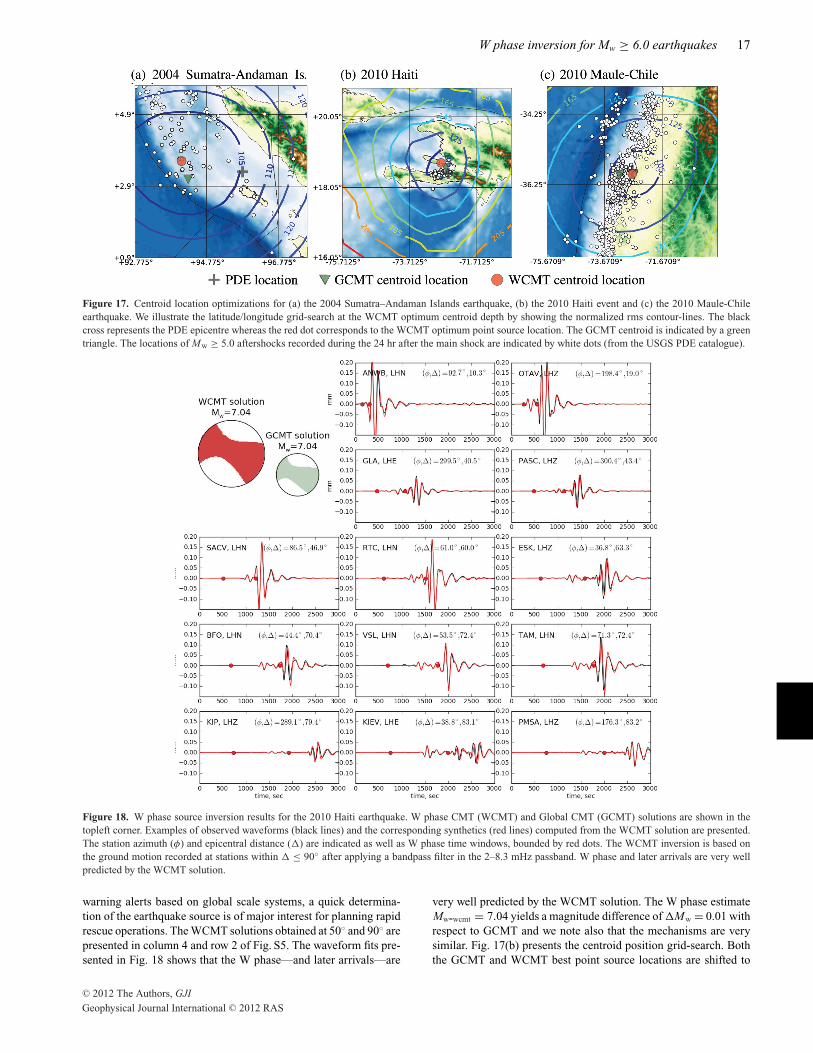
Figure 17. Centroid location optimizations for (a) the 2004 Sumatra–Andaman Islands earthquake, (b) the 2010 Haiti event and (c) the 2010 Maule-Chileearthquake. We illustrate the latitude/longitude grid-search at the WCMT optimum centroid depth by showing the normalized rms contour-lines. The blackcross represents the PDE epicentre whereas the red dot corresponds to the WCMT optimum point source location. The GCMT centroid is indicated by a greentriangle. The locations of Mw ! 5.0 aftershocks recorded during the 24 hr after the main shock are indicated by white dots (from the USGS PDE catalogue).

Figure 18. W phase source inversion results for the 2010 Haiti earthquake. W phase CMT (WCMT) and Global CMT (GCMT) solutions are shown in thetopleft corner. Examples of observed waveforms (black lines) and the corresponding synthetics (red lines) computed from the WCMT solution are presented.The station azimuth (!) and epicentral distance (") are indicated as well as W phase time windows, bounded by red dots. The WCMT inversion is based onthe ground motion recorded at stations within " " 90$ after applying a bandpass filter in the 2–8.3 mHz passband. W phase and later arrivals are very wellpredicted by the WCMT solution.

warning alerts based on global scale systems, a quick determina-tion of the earthquake source is of major interest for planning rapidrescue operations. The WCMT solutions obtained at 50$ and 90$ arepresented in column 4 and row 2 of Fig. S5. The waveform fits pre-sented in Fig. 18 shows that the W phase—and later arrivals—are

very well predicted by the WCMT solution. The W phase estimateMw-wcmt = 7.04 yields a magnitude difference of "Mw = 0.01 withrespect to GCMT and we note also that the mechanisms are verysimilar. Fig. 17(b) presents the centroid position grid-search. Boththe GCMT and WCMT best point source locations are shifted to



the north of the aftershock cloud. The great-circle distance betweenWCMT and GCMT centroids is about 20 km, with a small depthdifference of "rc , &1.5 km.

4.3.3 Example: 2010 Maule-Chile earthquake (Mw = 8.8, id =201002270634A)

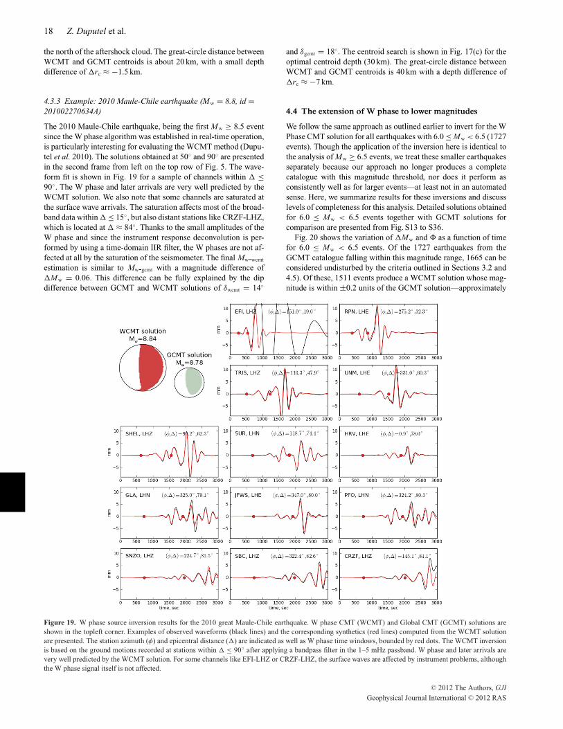
The 2010 Maule-Chile earthquake, being the first Mw ! 8.5 eventsince the W phase algorithm was established in real-time operation,is particularly interesting for evaluating the WCMT method (Dupu-tel et al. 2010). The solutions obtained at 50$ and 90$ are presentedin the second frame from left on the top row of Fig. 5. The wave-form fit is shown in Fig. 19 for a sample of channels within " "90$. The W phase and later arrivals are very well predicted by theWCMT solution. We also note that some channels are saturated atthe surface wave arrivals. The saturation affects most of the broad-band data within " " 15$, but also distant stations like CRZF-LHZ,which is located at " , 84$. Thanks to the small amplitudes of theW phase and since the instrument response deconvolution is per-formed by using a time-domain IIR filter, the W phases are not af-fected at all by the saturation of the seismometer. The final Mw-wcmt

estimation is similar to Mw-gcmt with a magnitude difference of"Mw = 0.06. This difference can be fully explained by the dipdifference between GCMT and WCMT solutions of +wcmt = 14$

and +gcmt = 18$. The centroid search is shown in Fig. 17(c) for theoptimal centroid depth (30 km). The great-circle distance betweenWCMT and GCMT centroids is 40 km with a depth difference of"rc , &7 km.

4.4 The extension of W phase to lower magnitudes

We follow the same approach as outlined earlier to invert for the WPhase CMT solution for all earthquakes with 6.0 " Mw < 6.5 (1727events). Though the application of the inversion here is identical tothe analysis of Mw ! 6.5 events, we treat these smaller earthquakesseparately because our approach no longer produces a completecatalogue with this magnitude threshold, nor does it perform asconsistently well as for larger events—at least not in an automatedsense. Here, we summarize results for these inversions and discusslevels of completeness for this analysis. Detailed solutions obtainedfor 6.0 " Mw < 6.5 events together with GCMT solutions forcomparison are presented from Fig. S13 to S36.

Fig. 20 shows the variation of "Mw and ( as a function of timefor 6.0 " Mw < 6.5 events. Of the 1727 earthquakes from theGCMT catalogue falling within this magnitude range, 1665 can beconsidered undisturbed by the criteria outlined in Sections 3.2 and4.5). Of these, 1511 events produce a WCMT solution whose mag-nitude is within ±0.2 units of the GCMT solution—approximately

Figure 19. W phase source inversion results for the 2010 great Maule-Chile earthquake. W phase CMT (WCMT) and Global CMT (GCMT) solutions areshown in the topleft corner. Examples of observed waveforms (black lines) and the corresponding synthetics (red lines) computed from the WCMT solutionare presented. The station azimuth (!) and epicentral distance (") are indicated as well as W phase time windows, bounded by red dots. The WCMT inversionis based on the ground motions recorded at stations within " " 90$ after applying a bandpass filter in the 1–5 mHz passband. W phase and later arrivals arevery well predicted by the WCMT solution. For some channels like EFI-LHZ or CRZF-LHZ, the surface waves are affected by instrument problems, althoughthe W phase signal itself is not affected.



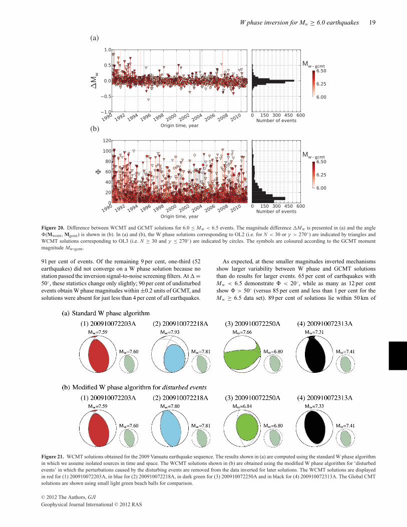
Figure 20. Difference between WCMT and GCMT solutions for 6.0 " Mw < 6.5 events. The magnitude difference "Mw is presented in (a) and the angle((Mwcmt, Mgcmt) is shown in (b). In (a) and (b), the W phase solutions corresponding to OL2 (i.e. for N < 30 or & > 270$) are indicated by triangles andWCMT solutions corresponding to OL3 (i.e. N ! 30 and & " 270$) are indicated by circles. The symbols are coloured according to the GCMT momentmagnitude Mw-gcmt.

91 per cent of events. Of the remaining 9 per cent, one-third (52earthquakes) did not converge on a W phase solution because nostation passed the inversion signal-to-noise screening filters. At " =50$, these statistics change only slightly; 90 per cent of undisturbedevents obtain W phase magnitudes within ±0.2 units of GCMT, andsolutions were absent for just less than 4 per cent of all earthquakes.

As expected, at these smaller magnitudes inverted mechanismsshow larger variability between W phase and GCMT solutionsthan do results for larger events. 65 per cent of earthquakes withMw < 6.5 demonstrate ( < 20$, while as many as 12 per centshow ( > 50$ (versus 85 per cent and less than 1 per cent for theMw ! 6.5 data set). 89 per cent of solutions lie within 50 km of

Figure 21. WCMT solutions obtained for the 2009 Vanuatu earthquake sequence. The results shown in (a) are computed using the standard W phase algorithmin which we assume isolated sources in time and space. The WCMT solutions shown in (b) are obtained using the modified W phase algorithm for ‘disturbedevents’ in which the perturbations caused by the disturbing events are removed from the data inverted for later solutions. The WCMT solutions are displayedin red for (1) 200910072203A, in blue for (2) 200910072218A, in dark green for (3) 200910072250A and in black for (4) 200910072313A. The Global CMTsolutions are shown using small light green beach balls for comparison.



GCMT centroid locations—very similar to the results for eventswith Mw ! 6.5. Interestingly, average depth differences for thesesmaller events are just 6.5 km when compared to GCMT solutions,and 90 per cent of the solutions obtain depth estimates within 12 kmof GCMT. These results suggest closer alignment with the GCMTresults than for the Mw ! 6.5 data set.

4.5 Disturbed events

As noted in Section 3.2, events that occur soon after another largeearthquake are problematic. We define ‘disturbed events’ as earth-quakes occurring within 1 hr of Mw ! 6.5 earthquakes or less than10 hr after Mw ! 7.0 events. These events have poor station az-imuthal coverage after performing the W phase data screening for" " 50$ (i.e. N < 30 or & > 270$). While the magnitude of a‘disturbed event’ is usually smaller than a preceding event (sincemost of them are aftershocks), this is not necessarily a rule, becausethere is no consideration of the size of earthquakes in the defini-tion of ‘disturbed events’. This makes such a definition particularlyadaptable for real-time operations of W phase inversions. To re-trieve the WCMT solution of such events in real time, Hayes et al.(2009) proposed to modify the time window and bandpass filter toperform a CMT inversion based on surface wave data. We explorehere an alternative approach in which we compute the synthetics forthe disturbing (preceding) event and subtract them from the data toproduce the residual trace. Then, we run the WCMT algorithm onthe residual trace to obtain the source parameters of the disturbedevent, as we do for a normal earthquake.

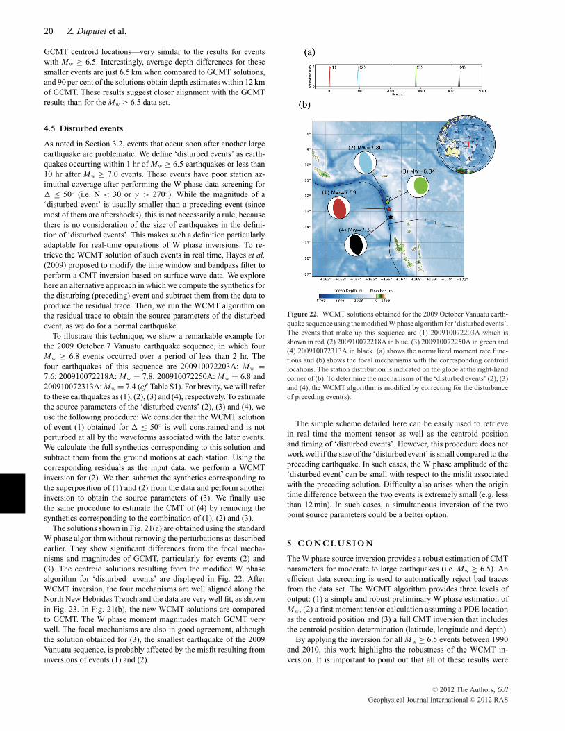
To illustrate this technique, we show a remarkable example forthe 2009 October 7 Vanuatu earthquake sequence, in which fourMw ! 6.8 events occurred over a period of less than 2 hr. Thefour earthquakes of this sequence are 200910072203A: Mw =7.6; 200910072218A: Mw = 7.8; 200910072250A: Mw = 6.8 and200910072313A: Mw = 7.4 (cf. Table S1). For brevity, we will referto these earthquakes as (1), (2), (3) and (4), respectively. To estimatethe source parameters of the ‘disturbed events’ (2), (3) and (4), weuse the following procedure: We consider that the WCMT solutionof event (1) obtained for " " 50$ is well constrained and is notperturbed at all by the waveforms associated with the later events.We calculate the full synthetics corresponding to this solution andsubtract them from the ground motions at each station. Using thecorresponding residuals as the input data, we perform a WCMTinversion for (2). We then subtract the synthetics corresponding tothe superposition of (1) and (2) from the data and perform anotherinversion to obtain the source parameters of (3). We finally usethe same procedure to estimate the CMT of (4) by removing thesynthetics corresponding to the combination of (1), (2) and (3).

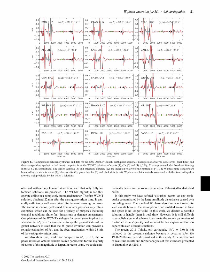
The solutions shown in Fig. 21(a) are obtained using the standardW phase algorithm without removing the perturbations as describedearlier. They show significant differences from the focal mecha-nisms and magnitudes of GCMT, particularly for events (2) and(3). The centroid solutions resulting from the modified W phasealgorithm for ‘disturbed events’ are displayed in Fig. 22. AfterWCMT inversion, the four mechanisms are well aligned along theNorth New Hebrides Trench and the data are very well fit, as shownin Fig. 23. In Fig. 21(b), the new WCMT solutions are comparedto GCMT. The W phase moment magnitudes match GCMT verywell. The focal mechanisms are also in good agreement, althoughthe solution obtained for (3), the smallest earthquake of the 2009Vanuatu sequence, is probably affected by the misfit resulting frominversions of events (1) and (2).

Figure 22. WCMT solutions obtained for the 2009 October Vanuatu earth-quake sequence using the modified W phase algorithm for ‘disturbed events’.The events that make up this sequence are (1) 200910072203A which isshown in red, (2) 200910072218A in blue, (3) 200910072250A in green and(4) 200910072313A in black. (a) shows the normalized moment rate func-tions and (b) shows the focal mechanisms with the corresponding centroidlocations. The station distribution is indicated on the globe at the right-handcorner of (b). To determine the mechanisms of the ‘disturbed events’ (2), (3)and (4), the WCMT algorithm is modified by correcting for the disturbanceof preceding event(s).

The simple scheme detailed here can be easily used to retrievein real time the moment tensor as well as the centroid positionand timing of ‘disturbed events’. However, this procedure does notwork well if the size of the ‘disturbed event’ is small compared to thepreceding earthquake. In such cases, the W phase amplitude of the‘disturbed event’ can be small with respect to the misfit associatedwith the preceding solution. Difficulty also arises when the origintime difference between the two events is extremely small (e.g. lessthan 12 min). In such cases, a simultaneous inversion of the twopoint source parameters could be a better option.

5 C O N C LU S I O N

The W phase source inversion provides a robust estimation of CMTparameters for moderate to large earthquakes (i.e. Mw ! 6.5). Anefficient data screening is used to automatically reject bad tracesfrom the data set. The WCMT algorithm provides three levels ofoutput: (1) a simple and robust preliminary W phase estimation ofMw, (2) a first moment tensor calculation assuming a PDE locationas the centroid position and (3) a full CMT inversion that includesthe centroid position determination (latitude, longitude and depth).

By applying the inversion for all Mw ! 6.5 events between 1990and 2010, this work highlights the robustness of the WCMT in-version. It is important to point out that all of these results were



Figure 23. Comparisons between synthetics and data for the 2009 October Vanuatu earthquake sequence. Examples of observed waveforms (black lines) andthe corresponding synthetics (red lines) computed from the WCMT solutions of events (1), (2), (3) and (4) (cf. Fig. 22) are presented after bandpass filteringin the 2–8.3 mHz passband. The station azimuth (!) and epicentral distance (") are indicated relative to the centroid of (4). The W phase time windows arebounded by red dots for event (1), blue dots for (2), green dots for (3) and black dots for (4). W phase and later arrivals associated with the four earthquakesare very well predicted by the WCMT solutions.

obtained without any human interaction, such that only fully au-tomated solutions are presented. The WCMT algorithm can thusoperate online in a completely automated manner. The first WCMTsolution, obtained 22 min after the earthquake origin time, is gen-erally sufficiently well constrained for tsunami warning purposes.The second inversion, performed 13 min later, provides very robustestimates, which can be used for a variety of purposes includingtsunami modelling, finite fault inversions or damage assessments.Completeness of the WCMT catalogue for recent years implies thatwherever an Mw > 6.5 event occurs today, the present status of theglobal network is such that the W phase inversion can provide areliable estimation of Mw and the focal mechanism within 35 minof the earthquake origin time.

We also show that, while not complete to Mw = 6.0, the Wphase inversion obtains reliable source parameters for the majorityof events of this magnitude or larger. In recent years, we could auto-

matically determine the source parameters of almost all undisturbedevents.

In this study, we have defined ‘disturbed events’ as any earth-quake contaminated by the large amplitude disturbance caused by apreceding event. The standard W phase algorithm is not suited forsuch events because the assumption of an isolated source in timeand space is no longer valid. In this work, we discuss a possiblesolution to handle them in real time. However, it is still difficultto establish a general scheme to estimate the source parameters of‘disturbed events’ quickly and we must further explore methods tocope with such difficult situations.

The recent 2011 Tohoku-oki earthquake (Mw = 9.0) is notincluded in the present catalogue because it occurred after the1990–2010 time period considered in this study. A detailed reportof real-time results and further analyses of this event are presentedin Duputel et al. (2011).



A C K N OW L E D G M E N T S

This work uses Federation of Digital Seismic Networks (FDSN)seismic data and CMT solutions from the Global CMT catalogue.The Incorporated Research Institutions for Seismology (IRIS) DataManagement System (DMS) was used to access the data. This workmade use of the Matplotlib python library. We thank J.-J. Leveque, J.Braunmiller, D. Garcia and an anonymous reviewer for their helpfulcomments on the manuscript.

R E F E R E N C E S

Abe, K., 1979. Size of great earthquakes of 1837–1974 inferred fromtsunami data, J. geophys. Res., 84, 1561–1568.

Abe, K., 1989. Quantification of tsunamigenic earthquakes by the Mt scale,Tectonophysics, 166(1–3), 27–34.

Abercrombie, R.E., 2003. The June 2000 Mw7.9 earthquakes south ofSumatra: deformation in the India–Australia Plate, J. geophys. Res., 108,2018, doi:10.1029/2001JB000674.

Ammon, C.J. et al., 2005. Rupture process of the 2004 Sumatra-AndamanEarthquake, Science, 308, 1133–1139.

Dahlen, F.A. & Tromp, J., 1998. Theoretical Global Seismology, PrincetonUniversity Press, Princeton, NJ.

Duputel, Z., Rivera, L. & Kanamori, H., 2010. W-phase: lessons from theFebruary 27, 2010 Chilean earthquake, Seismol. Res. Lett., 81, 544.

Duputel, Z., Rivera, L., Kanamori, H., Hayes, G.P., Hirshorn, B. & Weinstein,S., 2011. Real-time W phase inversion during the 2011 off the Pacific coastof Tohoku earthquake, Earth Planets Space, 63, 535–539.

Dziewonski, A., 1982. Harvard Centroid Moment Tensor Project, Availableat: http://www.globalcmt.org.

Dziewonski, A. & Woodhouse, J.H., 1983. Studies of the seismic sourceusing normal-mode theory, in Earthquakes: Observation Theory and In-terpretation: Notes from the International School of Physics “EnricoFermi” (1982: Varenna, Italy), pp. 45–137, North-Holland Publ. Co.,Amsterdam.

Dziewonski, A., Chou, T.A. & Woodhouse, J.H., 1981. Determination ofearthquake source parameters from waveform data for studies of globaland regional seismicity, J. geophys. Res., 86, 2825–2852.

Dziewonski, A.M. & Anderson, D.L., 1981. Preliminary reference Earthmodel, Phys. Earth planet. Inter., 25(4), 297–356.

Ekstrom, G. & Nettles, M., 2006. Global Centroid Moment Tensor Project,Available at: http://www.globalcmt.org.

Ekstrom, G., Dziewonski, A.M., Maternovskaya, N.N. & Nettles, M., 2005.Global seismicity of 2003: centroid–moment-tensor solutions for 1087earthquakes, Phys. Earth planet. Inter., 148(2–4), 327–351.

ERI, 2000. EIC Seismological Note 94, Technical report.Geist, E., 2005. Triggering of tsunamigenic aftershocks from large strike-

slip earthquakes: analysis of the November 2000 New Ireland earthquakesequence, Geochem. Geophys. Geosyst, 6, doi:10.1029/2005GC000935.

Hanks, T.C. & Kanamori, H., 1979. A moment magnitude scale, J. geophys.Res., 84, 2348–2350.

Hayes, G.P., Rivera, L. & Kanamori, H., 2009. Source inversion of theW-Phase: real-time implementation and extension to low magnitudes,Seismol. Res. Lett., 80, 817–822.

Hayes, G., Earle, P., Benz, H., Wald, D. & Briggs, R., 2011. 88 hours: TheUS Geological Survey National Earthquake Information Center responseto the March 11, 2011 Mw 9.0 Tohoku earthquake, Seismol. Res. Lett.,82, 481–493.

Hjorleifsdottir, V. & Ekstrom, G., 2010. Three-dimensional Earth structureon CMT earthquake parameters, Phys. Earth planet. Inter., 179, 178–190.

Kagan, Y.Y., 1991. 3-D rotation of double-couple earthquake sources, Geo-phys. J. Int., 106(3), 709–716.

Kanamori, H., 1972. Mechanism of tsunami earthquakes, Phys. Earth planet.Inter., 6, 356–359.

Kanamori, H., 1977. The energy release in great earthquakes, J. geophys.Res., 82(20), 2981–2987.

Kanamori, H., 1993. W phase, Geophys. Res. Lett., 20(16), 1691–1694.Kanamori, H., 2004. The diversity of the physics of earthquakes, Proc. Japan

Acad., 80, 297–316.Kanamori, H. & Anderson, D.L., 1975. Theoretical basis of some empirical

relations in seismology, Bull. seism. Soc. Am., 65, 1073–1095.Kanamori, H. & Given, J.W., 1981. Use of long-period surface waves for

rapid determination of earthquake-source parameters, Phys. Earth planet.Inter., 27, 8–31.

Kanamori, H. & Rivera, L., 2008. Source inversion of W phase: speedingup seismic tsunami warning, Geophys. J. Int., 175(1), 222–238.

Lay, T. et al., 2005. The great Sumatra-Andaman earthquake of 26 December2004, Science, 308, 1127–1133.

Lay, T., Ammon, C.J., Kanamori, H., Rivera, L., Koper, K. & Hutko, A.R.,2010. The 2009 Samoa-Tonga great earthquake triggered doublet, Nature,466(7309), 964–968.

Mendiguren, J.A., 1977. Inversion of surface wave data in source mechanismstudies, J. geophys. Res., 82(5), 889–894.

Okal, E.A., 1988. Seismic parameters controlling far-field tsunami ampli-tudes: a review, Nat. Hazards, 1(1), 67–96.

Park, J. et al., 2005. Earth’s free oscillations excited by the 26December 2004 Sumatra-Andaman earthquake, Science, 308(5725),1139–1144.

Park, S.-C. & Mori, J., 2007. Triggering of earthquakes during the 2000Papua New Guinea earthquake sequence, J. geophys. Res., 112(B3),B03302, doi:10.1029/2006JB004480.

Peterson, J., 1993. Observations and modelling of background seismic noise,Open-file Report 93-322, U.S. Geological Survey.

PTWC, 2006a. Tsunami Bulletin Number 001, Issued at 0836Z 17 Jul 2006,Technical report.

PTWC, 2006b. Tsunami Bulletin Number 002, Issued at 1108Z 17 July2006, Technical report.

Richter, C.F., 1935. An instrumental earthquake magnitude scale, Bull.seism. Soc. Am., 25(1), 1–32.

Rivera, L. & Kanamori, H., 2009. Using W phase for regional tsunamiwarning and rapid earthquake hazard assessment, in Proceedings of the2nd International Workshop on Earthquake Early Warning, Kyoto, Japan.

Rivera, L., Kanamori, H. & Duputel, Z., 2010. The potential of the W-phasealgoritm for regional tsunami warning in Chile, in Proceedings of AGUChapman Conference in Chile.

Silver, P.G. & Jordan, T.H., 1982. Optimal estimation of scalar seismicmoment, Geophys. J. R. astr. Soc., 70, 755–787.

Tsuruoka, H., Kawakatsu, H. & Urabe, T., 2009. GRiD MT (grid-basedreal-time determination of moment tensors) monitoring the long-periodseismic wavefield, Phys. Earth planet. Inter., 175(1–2), 8–16.

USGS, 2011. Report on the 2010 Haiti Earthquake, available athttp://earthquake.usgs.gov. (last accessed 2011 January).

A P P E N D I X : A N G U L A R D I S TA N C EB E T W E E N T W O M O M E N T T E N S O R S

To compare the orientations of the moment tensors MA and MB,we calculate the minimum angle necessary to bring the principalaxes of MB into coincidence with those of MA. This can be done asfollows. Let P(M) be the proper orthogonal matrix whose columnscorrespond to the principal axes of the moment tensor M. Becauseof the ambiguity in the principal axes directions there are four suchpossible matrices P1(M), P2(M), P3(M) and P4(M). We can fixP1(MA), compute the four angles

!k = cos&1 trace[P1(MA)Ptk(MB)] & 1

2, (A1)

and define ((MA, MB) = min[!1, !2, !3, !4] as the angular distancebetween MA and MB. This value ranges from 0$ to 120$. Thisdefinition is equivalent to the one given by Kagan (1991).



S U P P O RT I N G I N F O R M AT I O N

Additional Supporting Information may be found in the online ver-sion of this article:

Supplement. The Table S1 gives the complete list of disturbedevents considered in this study for Mw ! 6.5 (see Section 4.5 inthe main text). The complete collection of solutions obtained forMw ! 6.5 between 1990 and 2010 after rejecting the disturbedevents are shown in order of decreasing GCMT magnitude fromFig. S1 to Fig. S11. Each frame represents an earthquake for whichwe show the GCMT solution in green, and the W phase solu-tions incorporating stations within " " 50$ tb and within " "90$ at tc. WCMT mechanisms corresponding to OL2 (i.e. if N <

30 or & > 270$) are presented in blue while those correspond-ing to OL3 (i.e. if N ! 30$ and & " 270$) are shown in red.

N is the total number of channels after inversion and & is theazimuthal gap (in degrees). WCMT solutions for Mw ! 6.5 earth-quakes using data within " < 90$ are also available on the websitehttp://eost.u-strasbg.fr/wphase/MGE65. The great-circle distancesbetween WCMT, GCMT and PDE locations for Mw ! 6.5 earth-quakes are presented in Fig. S12 and the complete list of WCMTcentroid locations are listed from Table S2 to Table S15. The so-lutions resulting from the extension to 6.0 " Mw < 6.5 events(see Section 4.4 in the main text) are ordered in decreasing GCMTmagnitude Mw&gcmt from Fig. S13 to Fig. S36.

Please note: Wiley-Blackwell are not responsible for the content orfunctionality of any supporting materials supplied by the authors.Any queries (other than missing material) should be directed to thecorresponding author for the article.


Documents

W phase source inversion for moderate to large …wphase.unistra.fr/zacharie/papers/DuputelEtal2012a.pdfGeophys. J. Int. (2012) doi: 10.1111/j.1365-246X.2012.05419.x GJI Seismology