Geometry of Robotic Manipulation - cmp.felk.cvut.czcmp.felk.cvut.cz/cmp/courses/PRO/2011/Lecture/PRO... · Geometry of Robotic Manipulation Tom´aˇsPajdla [email protected]

Geometry of Robotic Manipulation

Tomas [email protected]

Monday 26th September, 2011

Contents

1 Notation 1

2 Linear algebra 22.1 Change of coordinates induced by the change of basis . . . . . . . . 2

3 Motion 63.1 Change of position vector coordinates induced by motion . . . . . . 63.2 Rotation matrix . . . . . . . . . . . . . . . . . . . . . . . . . . . . . 73.3 Coordinate vectors . . . . . . . . . . . . . . . . . . . . . . . . . . . . 11

Index 14

ii

1 Notation

� . . . the empty set [1]exp U . . . the set of all subset of set U [1]U � V . . . Cartesian product of sets U and V [1]Z . . . whole numbers [1]Q . . . rational numbers [2]R . . . real numbers [2]i . . . imaginary unit [2]�x . . . vectorA . . . matrixAij . . . ij element of AA� . . . transpose of A�A� . . . determinant of AI . . . identity matrixR . . . rotation matrixβ � ��b1,�b2,�b3� . . . basis (an ordered triple of independent generator vectors)�xβ . . . column matrix of coordinates of �x w.r.t. the basis β�x � �y . . . Euclidean scalar product of �x and �y (�x � �y � �x�β �yβ in an

orthonormal basis β)�x� �y . . . cross (vector) product of �x and �y

��x� . . . Euclidean norm of �x (��x� �

�x � �x)orthogonal vectors . . . mutually perpendicular and all of equal lengthorthonormal vectors . . . unit orthogonal vectors

1

2 Linear algebra

We rely on linear algebra [3, 4, 5, 6, 7, 8]. We recommend excellent text books [6, 3]for acquiring basic as well as more advanced elements of the topic. Monograph [4]provides a number of examples and applications and provides a link to numerical acomputational aspects of linear algebra. We will next review the most crucial topicsneeded in this text.

2.1 Change of coordinates induced by the change of basis

Let us discuss the relationship between the coordinates of a vector in a linear space,which is induced by passing from one basis to another. We shall derive the relation-ship between the coordinates in a three-dimensional linear space over real numbers,which is the most important when modeling the geometry around us. The formulasfor all other n-dimensional spaces are obtained by passing from 3 to n.

§1 Coordinates Let us consider an ordered basis β ��b1

�b2�b3

�of a three-

dimensional vector space V 3 over scalars R. A vector �v V 3 is uniquely expressedas a linear combination of basic vectors of V 3 by its coordinates x, y, z R, i.e.�v � x �b1 � y �b2 � z�b3, and can be represented as an ordered triple of coordinates,i.e. as �vβ �

�x y z

��.We see that an ordered triple of scalars can be understood as a triple of coorinates

of a vector in V 3 w.r.t. a basis of V 3. However, at the same time, the set ofordered tripples

�x y z

�� is also a three-dimensional coordinate linear space R3

over R with�x1 y1 z1

�� x2 y2 z2

�� x1 � x2 y1 � y2 z1 � z2

�� and

s�x y z

�� s x s y s z

�� for s R. Moreover, the ordered triple of thefollowing three particular coordinate vectors

β ��1

00

��

��0

10

��

��0

01

�� (2.1)

forms an ordered basis of R3, the standard basis, and therefore a vector �v � �x y z

��is represented by �vβ � �

x y z�� w.r.t. the standard basis in R3. It is noticable

that the vector �v and the coordinate vector �vβ of its coordinates w.r.t. the standardbasis of R3, are identical.

§2 Two bases Having two ordered bases β ��b1

�b2�b3

�and β� �

��b �1

�b �2�b �3

�leads to expressing one vector �x in two ways as �x � x �b1 � y �b2 � z �b3 and �x �x��b �1 � y��b �2 � z��b �3. The vectors of the basis β can also be expressed in the basis β�

2

T. Pajdla. Geometry of Robotic Manipulation 2011-9-26 ([email protected])

using their coordinates. Let us introduce

�b1 � a11�b �1 � a21

�b �2 � a31�b �3

�b2 � a12�b �1 � a22

�b �2 � a32�b �3 (2.2)

�b3 � a13�b �1 � a23

�b �2 � a33�b �3

§3 Change of coordinates We will next use the above equations to relate thecoordinates of �x w.r.t. the basis β to the coordinates of �x w.r.t. the basis β�

�x � x �b1 � y �b2 � z �b3

� x �a11�b �1 � a21

�b �2 � a31�b �3 � y �a12

�b �1 � a22�b �2 � a32

�b �3 � z �a13�b �1 � a23

�b �2 � a33�b �3

� �a11 x� a12 y � a13 z �b �1 � �a21 x� a22 y � a23 z �b �2 � �a31 x� a32 y � a33 z �b �3� x��b �1 � y��b �2 � z��b �3 (2.3)

Since coordinates are unique, we get

x� � a11 x� a12 y � a13 z (2.4)y� � a21 x� a22 y � a23 z (2.5)z� � a31 x� a32 y � a33 z (2.6)

Coordinate vectors �xβ and �xβ � are thus related by the following matrix multiplication��x�

y�

z�

��

��a11 a12 a13

a21 a22 a23

a31 a32 a33

��x

yz

�� (2.7)

which we concisely write as

�xβ� � A �xβ (2.8)

The columns of matrix A can be viewed as vectors of coordinates of basic vectors,�b1,�b2,�b3 of β in the basis β�

A ��

�b1β�

�b2β�

�b3β�

� � �

�� (2.9)

and the matrix multiplication can be interpreted as a linear combination of columnsof A by coordinates of �x w.r.t. β

�xβ� � x�b1β�� y�b2β�

� z�b3β�(2.10)

Matrix A plays such an important role here that it deserves its own name. MatrixA is very often called the change of basis matrix from basis β to β� or the transitionmatrix from basis β to basis β� [4, 9] since it can be used to pass from coordinatesw.r.t. β to coordinates w.r.t. β� by Equation 2.8.

However, literature [5, 10] calls A the change of basis matrix from basis β� to β,i.e. it (seemingly illogically) swaps the bases. This choice is motivated by the fact

3


that A relates vectors of β and vectors of β� by Equation 2.2 as��b1

�b2�b3

��

�a11

�b �1 � a21�b �2 � a31

�b �3 a12�b �1 � a22

�b �2 � a32�b �3

a13�b �1 � a23

�b �2 � a33�b �3

�(2.11)

��b1

�b2�b3

��

��b �1

�b �2�b �3

��a11 a12 a13

a21 a22 a23

a31 a32 a33

�� (2.12)

(2.13)

and threfore giving ��b1

�b2�b3

��

��b �1

�b �2�b �3

�A (2.14)

or equivalently ��b �1

�b �2�b �3

��

��b1

�b2�b3

�A�1 (2.15)

where the multiplication of a row of column vectors by a matrix from the right inEquation 2.14 has the meaning given by Equation 2.11 above. Yet another variationof the naming appeared in [7, 8] where A�1 was named the change of basis matrixfrom basis β to β�.

We have to conclude that the meaning associated with the change of basis matrixvaries in the literature and hence we will avoid this confusing name and talk aboutA as about the matrix transforming coordinates of a vector from basis β to basis β�.

There is the following interesting variation of Equation 2.14��

�b �1�b �2�b �3

�� A��

��

�b1

�b2

�b3

�� (2.16)

where the basic vectors of β and β� are understood as elements of column vectors.For instance, vector �b �1 is obtained as

�b �1 � aÆ11�b1 � aÆ12

�b2 � aÆ13�b3 (2.17)

where �aÆ11, aÆ12, aÆ13� is the first row of A��.Equations 2.2 and 2.14 tell us how to interpret columns of A. Similarly, Equa-

tion 2.15 provides the equaivalent interpretation of A�1.

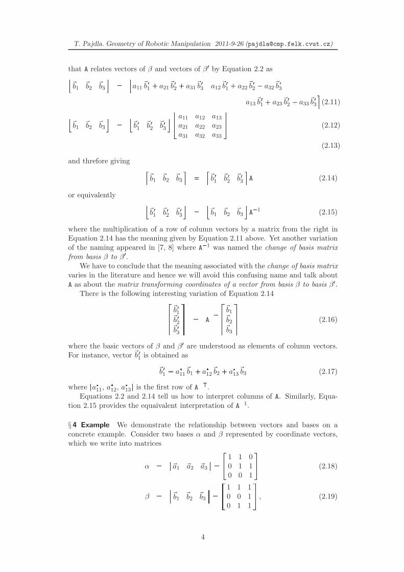
§4 Example We demonstrate the relationship between vectors and bases on aconcrete example. Consider two bases α and β represented by coordinate vectors,which we write into matrices

α � ��a1 �a2 �a3

� ��1 1 0

0 1 10 0 1

�� (2.18)

β ��b1

�b2�b3

��1 1 1

0 0 10 1 1

�� , (2.19)

4


and a vector �x with coordinates w.r.t. the basis α

�xα ��1

11

�� (2.20)

We see that basic vectors of α can be obtained as the following linear combinationsof basic vectors of β

�a1 � �1�b1 � 0�b2 � 0�b3 (2.21)�a2 � �1�b1 � 1�b2 � 1�b3 (2.22)�a3 � �1�b1 � 0�b2 � 1�b3 (2.23)

(2.24)

or equivalently

��a1 �a2 �a3

� ��b1

�b2�b3

��1 1 �10 �1 00 1 1

��

��b1

�b2�b3

�A (2.25)

Coordinates of �x w.r.t. β are hence obtained as

�xβ � A �xα, A ��1 1 �1

0 �1 00 1 1

�� (2.26)

�� 1�1

2

��

��1 1 �1

0 �1 00 1 1

��1

11

�� (2.27)

We see that

α � β A (2.28)��1 1 0

0 1 10 0 1

��

��1 1 1

0 0 10 1 1

��1 1 �1

0 �1 00 1 1

�� (2.29)

5

3 Motion

Let us introduce a mathematical model of rigid motion in three-dimensional Eu-clidean space. The important property of motion is that it only relocates objectswithout changing their shape. Distances between points on moving objects remainequal.

3.1 Change of position vector coordinates induced bymotion

X Y

�x

�x �

�y

�y �

O

O �

��o � �o �

�b1

�b2

�b �1

�b �2

Figure 3.1: Representation of rigid motion.

§5 Alias representation of motion1. Figure 3.1 illustrates a model of (rigid) motionusing coordinate systems, points and their position vectors. A coordinate system�O,β with origin O and basis β is attached to a moving rigid body. As the bodymoves to a new position, a new coordinate system �O �, β � is constructed. Assumea point X in a general position w.r.t. the body, which is represented in the frame�O,β by its position vector �x. The same point X is represented in the frame �O �, β � by its position vector �x �. The motion induces a mapping �xβ �� x �

β � . Such a mappingalso determines the motion itself and provides its convenient mathematical model.

1The terms alias and alibi were introduced in the classical monograph [11].

6


Let us derive the formula for the mapping �xβ �� x �

β � between the coordinates�x �

β � of vector �x � and coordinates �xβ of vector �x. Consider the following equations:

�x � �x � � �o � (3.1)�x � � �x � �o � (3.2)

�x �

β � � �xβ � � �o �

β � (3.3)

�x �

β � ��b1β �

�b2β �

�b3β �

� ��xβ � �o �

β

�(3.4)

�x �

β � � R��xβ � �o �

β

�(3.5)

�x �

β � � R �xβ � R�o �

β (3.6)�x �

β � � R �xβ � �o �

β � (3.7)�x �

β � � R �xβ � �oβ � (3.8)

Vector �x is the sum of vectors �x � and �o �, Equation 3.1. We can express all vectorsin (the same) basis β �, Equation 3.3. To pass to the basis β of the frame �O,β we introduce matrix R �

��b1β �

�b2β �

�b3β �

�, which transforms the coordinates of

vectors from β to β �, Eq. 3.4. Columns of matrix R are coordinates �b1β �,�b2β �

,�b3β �of

basic vectors �b1,�b2,�b3 of basis β in basis β �. Equations 3.6, 3.7, 3.8 present frequentvariations of the mapping. Notice that equation 3.8 introduced vector �o � ��o �.

§6 Alibi representation of motion. An alternative model of (rigid) motion canbe developed from the relationship between the points X and Y and their positionvectors in Figure 3.1. The point Y is obtained by moving point X altogether withthe moving object. It means that the coordinates �y �β � of the position vector �y � of Yin the coordinate system �O �, β � equal the coordinates �xβ of the position vector �xof X in the coordinate system �O,β , i.e.

�y �β � � �xβ

�yβ � � �oβ � � �xβ

R ��yβ � �oβ � �xβ

�yβ � R��xβ � �oβ (3.9)�yβ � R��xβ � �o �

β (3.10)

Equation 3.9 describes how is the point X moved to point Y w.r.t. the coordinatesystem �O,β .

3.2 Rotation matrix

Motion that leaves at least one point fixed is called rotation. Choosing such a fixedpoint as the origin leads to O � O � and hence to �o � �0. The motion is then fullydescribed by matrix R, which is called rotation matrix

§7 Two-dimensional rotation. To understand the matrix R, we shall start withan experiment in two-dimensional plane. Imagine a right-angled triangle ruler asshown in Figure 3.2(a) with arms of equal length and let us define a coordinate

7


�b1

�b1

�b2

�b2

�b �1

�b �2

a11

a11

�a21

a21

OO

(a) (b)

Figure 3.2: Rotation in two-dimensional space.

system as in the figure. Next, rotate the triangle ruler around its tip, i.e. around theorigin O of the coordinate system. We know, and we can verify it by direct physicalmeasurement, that thanks to the symmetry of the situation, the parallelogramsthrough the tips of �b1 and �b2 and along �b �1 and �b �2 will be rotated by 90 degrees. Wesee that

�b1 � a11�b �1 � a21

�b �2 (3.11)�b2 � a21

�b �1 � a11�b �2 (3.12)

for some real numbers a11 and a21. By comparing Equations 2.2, 2.8, and 3.8 weconclude that coordinates �xβ are transformed to coordinates �x �

β � (which actually areequal to coordinates �xβ � since �o � �0 in this case) as

�x �

β � �

a11 a21

�a21 a11

��xβ (3.13)

and thus

R �

a11 a21

�a21 a11

�(3.14)

We immediately see that

R�R �

a11 �a21

a21 a11

� a11 a21

�a21 a11

�� a2

11 � a221 0

0 a211 � a2

21

��

1 00 1

�(3.15)

since �a211 � a2

21 is the squared length of the basic vector of b1, which is one. Wederived an interesting result

R�1 � R� (3.16)R � R�� (3.17)

8


Figure 3.3: A three-dimensional coordinate system.

Next important observation is that for coordinates �xβ and �x �

β � , related by a rotation,there holds

�x� 2 � �y� 2 � �x �

β �

��x �

β � � �R �xβ � R �xβ � �x�β�R�R

��xβ � �x�β �xβ � x2 � y2 (3.18)

Now, if the basis β was constructed as in Figure 3.2, in which case it is calledorthonormal, then the parallelogram used to measure coordinates x, y of �x is arectangle and hence x2 � y2 is the squared length of �x by the Pythagoras theorem.If β � is related by rotation, then also �x� 2 � �y� 2 is the squared length of �x, againthanks to the Pythagoras theorem.

We see that �x�β �xβ is the squared length of �x when β is orthonormal and that thislength is preserved by computing it in the same way from the new coordinates of �xin the new coordinate system after motion. The change of coordinates induced bymotion is modeled by rotation matrix R, which has the desired property R�R � I,when the bases β, β � are both orthonormal.

§8 Three-dimensional rotation. Let us now think about three dimensions. Itwould be possible to generalize Figure 3.2 to three dimensions, construct orthonor-mal bases and use rectangular parallelograms to establish the relationship betweenelements of R in three dimensions. However, the figure and the derivations wouldbecome much more complicated.

We shall follow a more intuitive path instead. Consider that we have found thatwith two-dimensional orthonormal bases, the length of vectors could be computedby the Pythagoras theorem since the parallelograms determining the coordinateswere rectangular. To achieve this in three dimensions, we need (and can!) use basesconsisting from three orthogonal vectors. Then again the parallelograms will berectangular and hence the Pythagoras theorem for three dimensions can be usedanalogically as in two dimensions, Figure 3.3.

Considering orthonormal bases β, β � we require the following to hold for all

9


vectors �x with �xβ ��x y z

�� and �x �

β � ��x� y� z�

��

�x� 2 � �y� 2 � �z� 2 � x2 � y2 � z2

�x �

β �

��x �

β � � �x�β �xβ

�R �xβ � R �xβ � �x�β �xβ

�x�β�R�R

��xβ � �x�β �xβ

�x�β C �xβ � �x�β �xβ (3.19)

Equation 3.19 must hold for all vectors �x and hence also for special vectors such asthose with coordinates�

�100

�� ,

��0

10

�� ,

��0

01

�� ,

��1

10

�� ,

��1

01

�� ,

��0

11

�� (3.20)

Let us see what that implies, e.g., for the first vector

�1 0 0

�C

��1

00

�� 1 (3.21)

c11 � 1 (3.22)

Taking the second and the third vector similarly leads to c22 � c33 � 1. Now, let’stry the fourth vector

�1 1 0

�C

��1

10

�� 2 (3.23)

1� c12 � c21 � 1 � 2 (3.24)c12 � c21 � 0 (3.25)

Again, taking the fifth and the sixth vector leads to c13 � c31 � c23 � c32 � 0. Thisbrings us to the following form of C

C �� 1 c12 c13

�c12 1 c23

�c13 �c23 1

�� (3.26)

Moreover, we see that C is symmetric since

C� � �R�R

�� R�R � C (3.27)

which leads to �c12 � c12, �c13 � c13 and �c23 � c23, i.e. c12 � c13 � c23 � 0 andallows us to conclude that

R�R � C � I (3.28)

Interestingly, not all matrices R satisfying Equation 3.28 represent motions in three-dimensional space.

10


Consider, e.g., matrix

S ��1 0 0

0 1 00 0 �1

�� (3.29)

Matrix S does not correspond to any rotation of the space since it keeps the planexy fixed and reflects all other points w.r.t. this xy plane. We see that some matricessatisfying Equation 3.28 are rotations but there are also some such matrices thatare not rotations. Can we somehow distinguish them?

Notice that �S� � �1 while �I� � 1. It might be therefore interesting to studythe determinant of C in general. Consider that

1 � �I� � ��R�R �� R�� R� � �R� �R� � ��R� 2 (3.30)

which gives that �R� � �1. We see that the sign of the determinant splits allmatrices satisfying Equation 3.28 into two groups – rotations, which have positivedeterminant, and reflections, which have negative determinant. Product of any tworotations will again be rotation, product of a rotation and a reflection will be areflection and product of two reflections will be a rotation.

To summarize, rotation in three-dimensional space is represented by a 3 � 3matrix R with R�R � I and �R� � 1. The set of all such matrices, and at the sametime also the corresponding rotations, will be called SO�3 , for special orthonormalthree-dimensional. Two-dimensional rotations will be analogically denoted as SO�2 .

3.3 Coordinate vectors

We see that the matrix R induced by motion has the property that coordinatesand the basic vectors are transformed in the same way. This is particularly usefulobservation when β is formed by the standard basis, i.e.

β ��1

00

�� ,

��0

10

�� ,

��0

01

�� (3.31)

For motion Equation 2.16 becomes��

�b �1�b �2�b �3

�� R

��

�b1

�b2

�b3

��

��r11 r12 r13

r21 r22 r23

r31 r32 r33

��

�b1

�b2

�b3

��

��

r11�b1 � r12

�b2 � r13�b3

r21�b1 � r22

�b2 � r23�b3

r31�b1 � r32

�b2 � r33�b3

��(3.32)

and hence

�b �1 � r11�b1 � r12

�b2 � r13�b3 � r11

��1

00

�� r12

��0

10

�� r13

��0

01

��

��r11

r12

r13

��(3.33)

and similarly for �b �2 and �b �3. We conclude that

��b �1

�b �2�b �3

��

��r11 r21 r31

r12 r22 r32

r13 r23 r33

�� R� (3.34)

11


This also corresponds to solving for R in Equation 2.14 with A � R

��1 0 0

0 1 00 0 1

��

��b �1

�b �2�b �3

�R (3.35)

12

Bibliography

[1] Paul R. Halmos. Naive Set Theory. Springer-Verlag, 1974.

[2] Walter Rudin. Principles of Mathematical Analysis. McGraw-Hill, 1976.

[3] Paul R. Halmos. Finite-Dimensional Vector Spaces. Springer-Verlag, 2000.

[4] Carl D. Meyer. Matrix Analysis and Applied Linear Algebra. SIAM: Society forIndustrial and Applied Mathematics, Philadelphia, PA, USA, 2001.

[5] Petr Olsak. Uvod do algebry, zejmena linearnı. FEL CVUT, Praha, 2007.

[6] Pavel Ptak. Introduction to linear algebra. Vydavatelstvı CVUT, Praha, 2007.

[7] Gilbert Strang. Introduction to Linear Algebra. Wellesley Cambridge, 3rd edi-tion, 2003.

[8] Seymour Lipschutz. 3,000 Solved Problems in Linear Algebra. McGraw-Hill,1st edition, 1989.

[9] Jim Hefferon. Linear Algebra. Virginia Commonwealth University Mathematics,2009.

[10] Michael Artin. Algebra. Prentice Hall, Upper Saddle River, NJ 07458, USA,1991.

[11] Saunders MacLane and Garret Birkhoff. Algebra. Chelsea Pub. Co., 3rd edition,1988.

13

Index

coordinate linear space, 2

standard basis, 2

14

Documents

Geometry of Robotic Manipulation - cmp.felk.cvut.czcmp.felk.cvut.cz/cmp/courses/PRO/2011/Lecture/PRO... · Geometry of Robotic Manipulation Tom´aˇsPajdla [email protected]