Generic Mapping Tool (GMT)

2017+

K. Okino Atmosphere and Ocean Research Institute, The University of Tokyo

okino@aori.u-tokyo.ac.jp

rev. 2017.3.8

2

Course Outline 1 Introduction

1.1 GMT history 1.2 GMT outline 1.3 Goal of this course

2 How to use UNIX

2.1 UNIX overview 2.2 File System 2.3 Key commands and Tips 2.4 How to use awk

3 GMT First Step: Draw Map

3.1 Map Frame psbasemap -R -J -B -V 3.2 Draw coastline pscoast -D -W -G 3.3 How to use shell script -K -O

4 GMT Second Step: Draw topography/bathymetry map

4.1 Using grid data as input grdinfo 4.2 Draw contour map grdcontour 4.3 Draw color-fill map makecpt grdimage psscale 4.4 Draw shaded relief map grdgradient 4.5 Overlap two different dataset

5 GMT Third Step: Add symbols and lines

5.1 Draw symbols and lines psxy

6 GMT Forth Step: Plot time series data 6.1 Draw simple graph psxy –Jx gmtinfo 6.2 Draw time series data

7 GMT Fifth Step: Analysis and mathematics

7.1 Calculate the difference of two grid data grdmath 7.2 Filter data filter1d

3

8 GMT Forth Step: Display two different datasets 8.1 Gravity color map with topographic contours 8.2 Gravity color map on topographic shade

9 GMT Next Step:Making your own grid 9.1 Guideline for making grid 9.2 Making grid nearneighbor

Computer environment during lecture course

Linux XX GMT 5.1

GSView? NotePad++ emacs? Useful website GMT Project Home http://gmt.soest.hawaii.edu GMT latest document http://gmt.soest.hawaii.edu/doc/latest/index.html Global topography https://www.ngdc.noaa.gov/mgg/global/global.html (ETOPO1) Okino’s Tips&Script site (in Japanese) http://ofgs.aori.u-tokyo.ac.jp/~okino/gmtscripts/index.html

4

1. Introduction 1.1 GMT history 1.2 GMT overview 1.3 Goal of this course

2. How to use UNIX 2.1 UNIX Overview

2.2 File System

2.3 UNIX Key commands

At first, you need to open “terminal”. A black terminal window appears.

To investigate where you are in UNIX file system, type pwd↵ To see the list of file names in your present working directory, type ls↵ If you want to list up file names with more information, use option –l, ls -l ↵ Make new directory and check if new directory is really created. mkdir testdir↵

File System

/

home users work etc

BAMayKen

data doc

oceanland

aaa

bbb ccc

root

directory(folder)

pacific

file

zzz absolute path /home/May/zzz

absolute path: /home/Ken/data/ocean/ccc

you are here!

relative path: ccc

relative path: ../../May/zzzabsolute path: /home/Ken/data/ocean

5

ls ↵ Compare the list with desktop file browser. Then, change your position and check present working directory. cd testdir↵ pwd↵ Change your position: back to your previous (parent) directory. cd ..↵ pwd↵ Display contents of a file. cat testmap.bash↵ Copy the file. cp testmap.bash test-copy.bash↵ ls -l↵ cat test-copy.bash↵ Rename the file. mv test-copy.bash test-move.bash↵ ls -l↵ Delete the file. rm test-move.bash↵ rm test-copy.bash↵ ls -l↵ Redirect the output. cat testmap.bash > testout.bash↵ cat testout.bash↵ Look command history. history ↵ Try to use ↑key for repeating the previous command lines. OK, let’s start the GMT. Move to the lesson directory. cd lesson ↵

6

2.4 How to use awk AWK is a programming language for text processing, that is a standard feature of UNIX and UNIX-like operating systems. It is very useful to extract data, reformat data and so on. You can find many guide books and webpages to learn the details, however, we here try to learn the minimum technique to reformat data using a sample file.

Check the sample file “sample1.dat” in your home directory.

cat sample1.dat↵ The file has 10 lines and each line consists of nine values, (year month day hour min sec longitude latitude depth). Each value is separated by “blank”. Try to type the following line and see the result. awk ‘{print $7,$8}’ sample1.dat↵ You can extract only longitude and latitude data for all lines. Variable $X means Xth column of each line. Practice 1: Extract time (hour, min, sec) and depth and output to a new file. (use redirect “>”) Practice 2: You can perform mathematical operation (+, -, *, / etc.) between the variables. Try to output (hour, min=min+sec/60, -depth).

The part framed by ‘{ }’ is an AWK program (program includes only one command line). If you want to do much more complicated processing, you can save a group of command lines in one program file and use it. Let’s see a sample awk program “pos_min.awk”. cat pos_min.awk↵ You can see the lines below; { lon_deg=int($7); lon_min=($7-lon_deg)*60; lat_deg=int($8); lat_min=($8-lat_deg)*60; print $1,$2,$3,$4,$5,$6,$lon_deg,$lon_min,$lat_deg,$lat_min; }

7

# int($X) : round down to nearest decimal Try to run the program. awk –f pos_min.awk sample1.dat ↵ option –f filename: awk program is saved in filename.

You can also use “if else”, “do loop” etc. like C or Fortran languages and complicated text processing using regular expression. When you use this sample awk program for real dataset, there are at least two problems that should be solved; 1) how to deal with southern latitude and western longitude, 2) display digit. How to modify the file?

8

3 GMT First Step: Draw Map 3.1 Map Frame psbasemap -R -J -B

Try to create your first basemap (map frame) around Japan Islands. Type correctly the following line from command window.

gmt psbasemap -R135/145/30/40 –JM12 –Bf10ma1g30m –V > basemap1.ps↵

Check that the new file basemap1.ps is created in your home directory by type ls –l from terminal window. Then show the basemap1.ps using gv command.

gv basemap1.ps↵ You can see a map frame in gv window. “gv” is a program showing postscript files. The GMT “psbamsemap” command draws a map frame, defined by various options. Above, we only used four options,

-R map region west/east/south/north degree or deg:min:sec -J map projection Mlength or mscale : Mercator Projection -B frame option f: tick interval a: annotation interval g: grid interval -V verbose option

Access the GMT official web site below.

http://gmt.soest.hawaii.edu/doc/latest/index.html You can read manual pages, cookbook, and other documents from this site. Click the link CookBook 13 GMT Map Projections. You can see available map projections and the usage.

Practice 1: Change region: western boundary ->125°E northern ->45°N Practice 2: Change scale to 1:10000000 Practice 3: Change projection to Lambert Azimuthal Equal-Area

projection Practice 4: Change boundary details: Tick interval is 1°, annotation interval is 5°, grid interval is 1°

3.2 Draw coastline pscoast -D -W -G

Try to draw coastlines around Japan Islands. Type

9

gmt pscoast -R125/145/30/45 –JM12 –Bf1a5g5 –Di –Ggray –Wthin,black –V > coastmap1.ps↵

Check the coastmap1.ps using gv. -D map resolution (f)ine h(igh) (i)ntermediate (l)ow -G map fill color or pattern for “dry” “land” area -W pen attribute pen width and color for coastline

pen width: Pen and paint color: See CookBook 22 Color Space. Practice 1: Change map resolution : try lowresolution Practice 2: Change land color: green Practice 3: Change pen attribute: thick, blue Practice 4: Read GMT online manual pscoast and add political boundary Practice 5: Try to delete –B option, what happens?

3.3 How to use shell script -K –O

When you want to make a more complicated map using multiple GMT commands, you need to execute a series of commands sequentially. Type

gmt pscoast -R125/145/30/45 –JM15 –Di –Ggray –Wthin,black –V –K > coastbasemap1.ps↵

Check the output file coastbasemap1.ps by ls –l command. Then see the map by gv. There is no map frame, for the command line lacks –B option. Then, type

gmt psbasemap -R125/145/30/45 –JM15 –Bf1a5g5 –V –O >> coastbasemap1.ps↵

faint 0 thicker 1.5p default 0.25p thickest 2p thinnest 0.25p fat 3p thinner 0.50p fatter 6p thin 0.75p fattest 12p thick 1.0p obese 18p

10

!! attention !! output file name is the same. redirection is not >, type “>>” (append)

Again, check the size of coastbasemap1.ps by ls –l. Does the file size increase? . The output of two commands are pasted, creating one ps file. Then see the map by gv.

-K another script is appended after the command -O another script exists before the command

shell script

Typing a series of command lines is always troublesome. Writing a “shell script” is a smart way of using GMT. Open the sample shell script plot_coast.bash in your directory using gedit.

gedit plot_coast.bash↵ #! /bin/bash # this line depends on your system # parameter setting region=125/145/30/45 proj=M15 frame=f1a5g5 psfile=coastbasemap2.ps # gmt pscoast –R$region –J$proj –Di –Ggray –Wthin,black –K –V > $psfile gmt psbasemap –R$region –J$proj –B$frame –O –V >> $psfile #

From your window, try to type the following. ./plot_coast.bash ↵

Is coastbasemap2.ps created successfully? Practice: Copy your first script plot_coast.bash to make a new script (you can use your favorite name, but extension “.bash” is recommended). Change region, boundary, projection, color etc. to make your own country/region map.

11

4. GMT Second Step: Draw topography/bathymetry map 4.1. Using grid data as input grdinfo

GMT can manipulate ascii/binary tables and gridded data. Grid data mainly used in GMT is netCDF format, consisting a header part and array of numbers. Let’s draw topography map using a topography grid file. You can find a grid file named japan_etopo2.grd in your disk. The grid file format is netCDF, so you cannot open/display the contents of file by cat command or text editors.

From your window, try to type the following.

gmt grdinfo japan_etopo2.grd ↵ You can see the detail information of the grid.

4.2. Draw contour map grdcontour -C

Let’s draw a contour map using the above gridded topography data and grdcontour command. Again, copy plot_coast.bash and make a new script. Open the new script in gedit and change/add the following lines in red.

#! /bin/bash # parameter setting region=125/145/30/45 proj=M15 frame=f1a5g5 grdfile=japan_etopo2.grd psfile=contour.ps # gmt grdcontour $grdfile –R$region –J$proj –C200 –A1000 –K –V > $psfile gmt pscoast –R$region –J$proj –Di –Ggray –Wthin,black –K –V –O >> $psfile gmt psbasemap –R$region –J$proj –B$frame –O –V >> $psfile #

Run the script. For grdcontour, -C option defines contour interval and –A option defines annotated contour interval. Don’t forget putting both –K and –O for pscoast, for another gmt command appears both before and after pscoast.

Practice: Change contour interval to 500m.

4.3. Draw color-fill map makecpt grdimage psscale Let’s draw a color-fill map using grdimage command. You first need to make color palette table by makecpt command (in GMT world, color palettes are usually named as ***.cpt). GMT system includes many standard color palettes and you can choose

12

one of them and fit the color scale to your dataset. Open the previous script, comment out the grdcontour (add # at beginning of the line), and add grdimage command. Adding comment or note using # is useful for readable scripts.

#! /bin/bash # parameter setting region=125/145/30/45 proj=M15 frame=f1g5a5

grdfile=japan_etopo2.grd psfile=colorfill.ps cptfile=topocol.cpt # # making color table gmt makecpt –Ctopo –T-8000/4000/1000 –Z > $cptfile # # drawing color-fill map gmt grdimage $grdfile –R$region –J$proj –C$cptfile –K –V > $psfile gmt psscale –D16/3/10/0.5 –C$cptfile –K –O >> $psfile # gmt grdcontour $grdfile –R$region –J$proj –C100 –A1000 –K –V > $psfile gmt pscoast –R$region –J$proj –Di –Ggray –Wthin,black –K –V –O >> $psfile gmt psbasemap –R$region –J$proj –B$frame –O –V >> $ofile #

Run the script. For makecpt command, -C option defines system color palette and -T option defines the min/max/interval values for the color palette. You can check built-in color palette from CookBook 26 Of colors and Color Legends. For grdimage command, -C option defines the color palette table you want to use. Command psscale plots color legend bar, where -D option defines the position and size of the legend. After running this script, you find the land area in gray. If you want to use your own color table both for land and ocean, delete the -G option of pscoast.

Practice 1 : By using online manual, check the meaning of “-Z” option of makecpt. Then try to remove the –Z option and run the script. Practice 2: Change the color palette. Try to use one of other system color palettes and define the limit. You can see the list of system color palette by typing makecpt or access the CookBook. Practice 3: How to draw a color map with contours? Remove the “#” of grdcontour command line and then ??

13

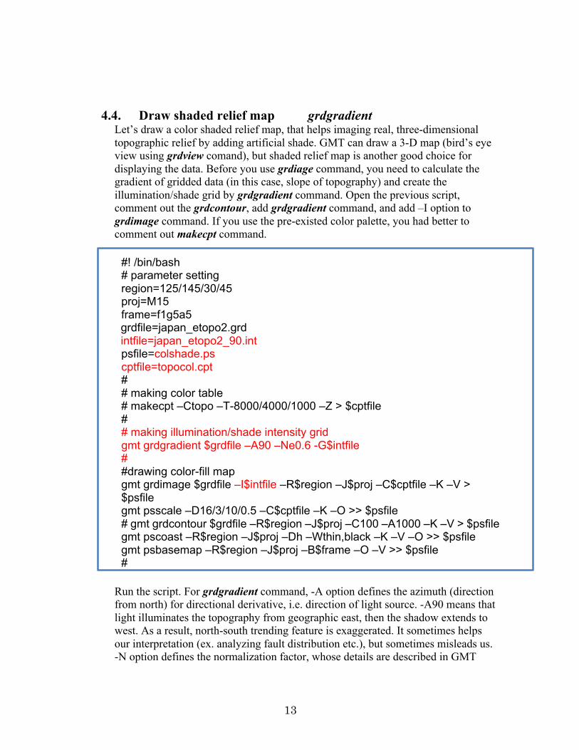
4.4. Draw shaded relief map grdgradient

Let’s draw a color shaded relief map, that helps imaging real, three-dimensional topographic relief by adding artificial shade. GMT can draw a 3-D map (bird’s eye view using grdview comand), but shaded relief map is another good choice for displaying the data. Before you use grdiage command, you need to calculate the gradient of gridded data (in this case, slope of topography) and create the illumination/shade grid by grdgradient command. Open the previous script, comment out the grdcontour, add grdgradient command, and add –I option to grdimage command. If you use the pre-existed color palette, you had better to comment out makecpt command.

#! /bin/bash # parameter setting region=125/145/30/45 proj=M15 frame=f1g5a5

grdfile=japan_etopo2.grd intfile=japan_etopo2_90.int

psfile=colshade.ps cptfile=topocol.cpt # # making color table # makecpt –Ctopo –T-8000/4000/1000 –Z > $cptfile # # making illumination/shade intensity grid gmt grdgradient $grdfile –A90 –Ne0.6 -G$intfile # #drawing color-fill map gmt grdimage $grdfile –I$intfile –R$region –J$proj –C$cptfile –K –V > $psfile gmt psscale –D16/3/10/0.5 –C$cptfile –K –O >> $psfile # gmt grdcontour $grdfile –R$region –J$proj –C100 –A1000 –K –V > $psfile gmt pscoast –R$region –J$proj –Dh –Wthin,black –K –V –O >> $psfile gmt psbasemap –R$region –J$proj –B$frame –O –V >> $psfile #

Run the script. For grdgradient command, -A option defines the azimuth (direction from north) for directional derivative, i.e. direction of light source. -A90 means that light illuminates the topography from geographic east, then the shadow extends to west. As a result, north-south trending feature is exaggerated. It sometimes helps our interpretation (ex. analyzing fault distribution etc.), but sometimes misleads us. -N option defines the normalization factor, whose details are described in GMT

14

command reference. To make intensity file for grdimage, -Ne0.6 is a good choice for first try.

Practice 1 : Change the normalization factor. Practice 2: Change the light direction. You can also chose two light sources as –A0/90. Practice 3: Create your shaded relief map with contours of your own country/region.

15

5. GMT Third Step: Add symbols and lines 5.1. Draw symbols and lines psxy

GMT can read ascii/binary table and plot the symbols and lines. Try to plot sampling points and survey lines on white map. Test datasets named sample_loc.dat and line_loc.dat are included in your disk. These datasets are ascii file, so you can check the contents by cat command.

Copy your first script plot_coast.bash and make a new script. Open the new script and add new parameters and two psxy command lines.

#! /bin/bash # parameter setting region=125/145/30/45 proj=M15 frame=f1a5g5 pointfile=sample_loc.dat linefile=line_loc.dat psfile=locationmap.ps # gmt pscoast –R$region –J$proj –Dh –Ggray –Wthin,black –K –V > $psfile gmt psxy $pointfile –R$region –J$proj –Sa0.2 –Gred –K –O –V >> $psfile gmt psxy $linefile –R$region –J$proj –Wthick,blue –K –O –V >> $psfile gmt psbasemap –R$region –J$proj –B$frame –O –V >> $psfile #

Run the script. For psxy command, -S option defines the type and size of the symbols. Without -S option, GMT draws lines linking input points. -G (fill_color) and/or -W (pen attribute for symbol outline) are requested. Refer the online manual page of psxy for checking the symbol types.

Practice 1: Change symbol type and size as you like. Practice 2: Change symbol or line colors. Try to add outlines of symbols using -W option.

16

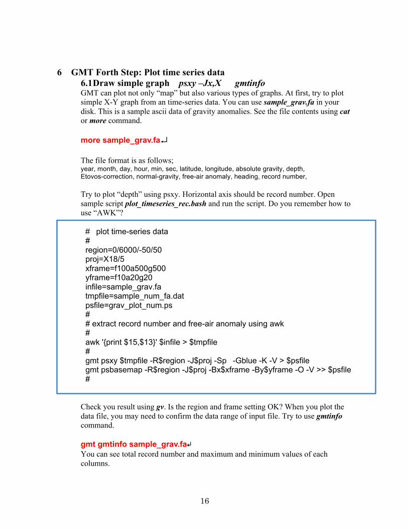
6 GMT Forth Step: Plot time series data 6.1 Draw simple graph psxy –Jx,X gmtinfo GMT can plot not only “map” but also various types of graphs. At first, try to plot simple X-Y graph from an time-series data. You can use sample_grav.fa in your disk. This is a sample ascii data of gravity anomalies. See the file contents using cat or more command. more sample_grav.fa↵ The file format is as follows; year, month, day, hour, min, sec, latitude, longitude, absolute gravity, depth, Etovos-correction, normal-gravity, free-air anomaly, heading, record number, Try to plot “depth” using psxy. Horizontal axis should be record number. Open sample script plot_timeseries_rec.bash and run the script. Do you remember how to use “AWK”?

# plot time-series data # region=0/6000/-50/50 proj=X18/5 xframe=f100a500g500 yframe=f10a20g20 infile=sample_grav.fa tmpfile=sample_num_fa.dat psfile=grav_plot_num.ps # # extract record number and free-air anomaly using awk # awk '{print $15,$13}' $infile > $tmpfile # gmt psxy $tmpfile -R$region -J$proj -Sp -Gblue -K -V > $psfile gmt psbasemap -R$region -J$proj -Bx$xframe -By$yframe -O -V >> $psfile #

Check you result using gv. Is the region and frame setting OK? When you plot the data file, you may need to confirm the data range of input file. Try to use gmtinfo command. gmt gmtinfo sample_grav.fa↵ You can see total record number and maximum and minimum values of each columns.

17

Practice 1: Change the script to show heading data. Practice 2: Plot “depth data”. Depth values are positive in the input file (downward positive), but upward positive plot maybe better to understand.

6.2 Draw time series data The previous plot used “record number” as horizontal axis. We then try to change the horizontal axis to “TIME”. GMT can produce time-series plot in several ways; easiest way is to calculate total seconds since the epoch (UNIT time or the start time of survey….) and to use it as horizontal axis. Here we learn how to display day, hour, min etc. in horizontal axis. The script plot_timeseries_hour.bash consists of two steps; 1) reformat (year,mon,day,hour,min,sec) data to fit standard time-series format（yyyy-mm-ddThh:mi:ss） using awk program file, and 2) plot data using option –Bt. Try to run the script and check awk file, awk output, and the resulting plot.

fa2ts.awk

{ printf("%4d-%02d-%02dT%02d:%02d:%02d %7.1f\n",$1,$2,$3,$4,$5,$6,$13); }

# plot time-series data # infile=sample_grav.fa tsfile=sample_grav.ts start_ts=2016-01-23T00:00:00 end_ts=2016-01-24T00:00:00 region=$start_ts/$end_ts/-100/100 proj=X18/5 xframe=f1ha4hg4h yframe=f10a20 psfile=grav_plot_ts.ps # # reformat input file using awk program "fa2ts.awk" # awk -f fa2ts.awk $infile > $tsfile # gmt psxy $tsfile -R$region -J$proj -Sp -Gblue -K -V > $psfile gmt psbasemap -R$region -J$proj -Bx$xframe -By$yframe -O -V >> $psfile

18

Practice 1: To check the data quality more precisely, enlarge the plot. Display only 12:00 -16:00 data and add appropriate frame tick marks and annotations. See online manual, http://gmt.soest.hawaii.edu/doc/5.1.0/gmt.html#the-common-gmt-options

19

7 GMT Fifth Step: Analysis and mathematics 7.1 Calculate the difference of two grid data grdmath You can do grid data calculation (add, subtract, multiply etc.) using grdmath command. There are two sample datasets in your lesson folder, tarama_mb.grd and tarama_etopo.grd. Investigate the grid specification of these files using grdinfo. gmt grdinfo tarama_mb.grd↵ gmt grdinfo tarama_etopo.grd↵

The range (region) and grid interval settings are same. The tarama_mb file contains bathymetry collected by ship sonar, and tarma_etopo file contains bathymetry predicted from satellite altimetry. You can calculate the difference of these two files using grdmath. gmt grdmath tarama_mb.grd tarama_etopo.grd SUB = tarama_diff.grd↵ Practice 1: Plot original two files (_mb, etopo) and difference file (diff). Practice 2: Create new grid file that contains the difference of two files in percentage of original (_etopo) file.

7.2 Filter data filter1d GMT includes some filtering command both for grid and table data. Here we try to run filter1d, using sample_num_fa.dat created during chapter 6.1. The sample script test_filt.bash will execute Boxcar filtering (=simple moving average) of data. Copy plot_timeseries_rec.bash to new script file and add lines below. Try to run the script and confirm the result.

# plot time-series data # region=0/6000/-50/50 proj=X18/5 xframe=f100a500g500 yframe=f10a20g20 infile=sample_grav.fa tmpfile=sample_num_fa.dat psfile=grav_plot_num.ps # # extract record number and free-air anomaly using awk# # awk '{print $15,$13}' $infile > $tmpfile

20

# gmt psxy $tmpfile -R$region -J$proj -Sp -Gblue -K -V > $psfile gmt psbasemap -R$region -J$proj -Bx$xframe -By$yframe -K -O -V >> $psfile # # box car filtering # filtfile=sample_num_fa_b50.dat gmt filter1d $tmpfile -Fb50 -N0 -V > $filtfile gmt psxy $filtfile -R$region -J$proj -Sp -Gred -O -V >> $psfile

Practice 1: Change the filter type and width as you like. See online manual for details.

21

8. GMT Sixth Step: Display two different datasets You may sometimes want to display two different datasets and investigate the relationship between them. Let’s consider to display gravity anomaly and topography together. You can use japan_etopo2.grd and japan_altgrv.grd in your disk.

8.1 Draw gravity anomaly map with topographic contours

Practice 1: Draw gravity anomaly color-fill map. First, try to draw gravity anomalies. You can use the previous script for making color-fill topography map. Revise the script for plotting gravity anomaly. You may need to make new color table to display gravity grid. Before writing the script, you had better to check the minimum and maximum value of gravity anomaly data using grdinfo command (then, you can set appropriate parameters for makecpt –T option). Practice 2: Add topography contours on gravity color map. Add grdcontour command after grdimage command. Choose appropriate contour interval (too dense contours is not good). Practice 3: Try to add gravity anomaly contours in different color Add another grdcontour command to display gravity anomaly contours. You had better to choose different pen attributes (thickness and color) for bathymetry and gravity.

8.2 Draw gravity anomaly map with topographic shade When we create a shade relief map, grdimage command requires two input gridded data files, one for color-fill and one for shading. In the previous practice, the intensity file (for shading) is calculated from the same grid for color-fill. Now, try to use gravity data for color-fill and topography data for shading (–I). The result shows gravity color map drapes over topography relief.

Practice: Revise your previous script for making shaded relief map. Define two different input grid files and select appropriate color table.

22

9 GMT Next Step: Making your own grid data In previous practices, we use open topography/gravity data. You may need to plot your own data based on your own surveys. If the survey/sampling point is very limited, you can display the observed values using psxy, for symbol sizes or colors can be varied with values (refer psxy manual page). If your data exist widely over the target area and you want to make color-fill or contour map of your data, what you should do is to create a gridded data file from discrete observations.

9.1 Guide line for making grid

To make your own grid, what you need to consider first is to decide the grid interval (grid size). There is no general rule for deciding the grid interval. You can choose minimum grid interval, where only one data point exists in one grid. You can also choose larger grid interval, averaging multiple raw data values. It depends on circumstances.

Let’s use the sample data ship.xyz. This file includes arbitrarily spaced bathymetry data in Baja California. (this sample file is delivered in GMT package as examples). Check the contents using the following two unix/gmt commands.

head ship.xyz ↵ gmt info ship.xyz↵

Open the sample script gridmaking.bash and run the script. Look up the output file point_plot.ps. Let’s investigate the script. The first section of the script is to display the distribution of data points by psxy.

# parameter setting region=245/255/20/30 proj=M15 frame=f10ma30mg1 xyzfile=ship.xyz grdfile=ship_5m.grd psfile=ship_cont.ps # # first step: just plot gmt psxy $xyzfile –R$region –J$proj –Sp –K –V > $psfile gmt pscoast –R$region –J$proj –Dh –Ggray –Wthick,black –K –V –O >> $psfile gmt psbasemap –R$region –J$proj –B$frame –O –V >> $psfile

23

# # second step: gridding # #grdint=5m #sradius=40k # #gmt nearneighbor $xyzfile –R$region –I$grdint –S$sradius –G$grdfile –V #gmt grdcontour $grdfile –R$region –J$proj –C200 –A1000 –K –V > $psfile #gmt pscoast –R$region –J$proj –Dh –Ggray –Wthick,black –K –V –O >> $psfile #gmt psbasemap –R$region –J$proj –B$frame –O –V >> $psfile #

9.2 Making grid nearneighbor

Now, try to make 5’ x 5’ (arcmin) interval grid data from ship.xyz. Open the previous script gridmaking.bash and comment out the first step command lines and delete # of lines in second step. The nearneighbor command reads arbitrarily located data points (x,y,z) and uses a nearest neighbor algorithm to assign an average value to each node that have one or more points within a radius centered on the node. The average value is computed as a weighted mean of the nearest point from each sector (quadrant in default) inside the search radius. Weight is a function of distance from the node.

(from GMT cookbook) Try to run the script and check the result. You can get your own grid file and contour map! Another way of making grid is to use surface command, that creates gridded data using adjustable tension continuous curvature splines. When you manipulate potential data like gravity/magnetic anomalies.