Generalizations of powerlaw distributions applicable to sampled

Generalizations of power-law distributions applicable to sampledfault-trace lengths: model choice, parameter estimation and caveats

R.M. Clark,1 S. J. D. Cox2 andG.M. Laslett31 Department of Mathematics and Statistics, Monash University, Clayton, Victoria 3168, Australia. E-mail: [email protected] Australian Geodynamics Cooperative Research Centre, CSIRO Exploration and Mining, PO Box 437, Nedlands,WA 6009, Australia3 CSIROMathematical and Information Sciences, Private Bag 10, Clayton South MDC, Clayton, Victoria 3169, Australia

Accepted 1998 August 28. Received 1998 August 24; in original form 1997 November 10

SUMMARYIt has often been observed that fault-trace lengths tend to follow a power-law or Paretodistribution, at least for su¤ciently large lengths. A very common method of ¢tting thistype of model to data consists of plotting on log^log axes the number of faults with tracelength greater than x against x, and reading o¡ the slope of the resulting approximatestraight line. We demonstrate that maximum likelihood is a more e¤cient and lessbiased method of estimating the power-law exponent.

A further complication is that this log^log plot is often curved, suggesting thatthe power-law distribution is not a complete description of the data. In this paper wereview the literature on probability distributions with Pareto behaviour for long tracelengths, but not necessarily for short trace lengths. The Feller^Pareto distribution is anattractive family within this class, with many well-known statistical distributions asspecial cases. We use maximum likelihood to ¢t the Feller^Pareto distribution to asample of 1034 fault-trace lengths from the South Yorkshire coal¢elds. We concludethat the Burr III model super¢cially provides a satisfactory ¢t to these data. We alsodiscuss an interpretation of the Feller^Pareto model in terms of a particular type ofobservational bias on data generated from the power-law distribution.

However, there are a number of complications to be considered. In particular, geo-metrical sampling biases, stereological e¡ects and spatial structure in the data meanthat a rigorous analysis is not straightforward. We suggest ways in which future datacollection and analysis may address some of these problems.

If our sampling protocols and estimation procedures are adopted, geoscientists shouldbe able to estimate the power-law exponent more accurately and more objectively thanwith current ad hoc procedures, andwith more direct relevance to strain calculations andother geophysical applications. Furthermore, our recommended method of estimation,maximum likelihood, provides point estimates and associated standard errors of theunknown parameters, and is e¤cient, consistent and relatively straightforward to apply.

Key words: b value, fault models, faulting, fractals, statistical methods.

1 INTRODUCTION

Faults are an important class of linear features in geology. Inmany instances, groups of faults act together to control thedeformation behaviour of rock masses. In order to understandthis behaviour properly, it is often useful to analyse the faults interms of their population statistics.Following the well-known Gutenberg^Richter frequency^

magnitude relation for earthquake populations, similar power-law relationships have been described in a large number ofstudies of the size distribution of geological faults [plus otherfeatures such as ore deposits (Agterberg 1995)]. A recentspecial issue of the Journal of Structural Geology (Vol. 18,

Issues 2/3, 1996) includes a number of papers related to this. Aprodigious amount of e¡ort has been devoted to establishingpower-law models for faults. There are a number of unresolvedissues, speci¢cally:

(1) Can a single power-law exponent be used to describe allgroups of faults?(2) Is the power-law exponent constant over the complete

scale range? And if not, then what can be deduced from thevariations?

These questions are important since the distribution of faultsizes gives us valuable information about the mechanics of thesystem during formation. In particular, it has been suggested

Geophys. J. Int. (1999) 136, 357^372

ß 1999 RAS 357

Dow

nloaded from https://academ

ic.oup.com/gji/article/136/2/357/694092 by guest on 28 N

ovember 2021

(Pacheco et al. 1992; Davy 1993; Westaway 1994; Scholz 1995)that changes in the exponents of the power-law distributionsindicate di¡erent regimes of boundary conditions: for example,the transition from 3-D bounded faults completely enclosedwithin a layer to 2-D bounded faults when they are largeenough to intersect the limits of the layer, particularly at thebase of the brittle crust. There are a number of sets of faultsand fractures in important parts of Australia for which such ameasurement would give a new and unique constraint on thegeometry of the critical mechanical elements for particularperiods in geological history: the early Proterozoic dyke suitein the Yilgarn block (Isles & Cooke 1990) and the extensivefracture set in the Arnhem Land plateau (Fitton & Cox 1995)are two spectacular examples.In a recent paper, Clark & Cox (1996) showed that the use of

correct statistical procedures can make a signi¢cant contri-bution to resolving a related issue (the relation between faultsize and displacement). We believe that this is also the case forthe size distribution problem. In particular, in this paper wedemonstrate that generalized forms of the usual power-lawrelation, known as Feller^Pareto distributions, provide a gooddescription of real data sets. These distributions include termswhich can be related to various forms of sampling bias thatmay contaminate the observations.Also, by using modern statistics it is possible to take

into account various practical sampling problems, such ascensoring, edge e¡ects and truncation.

2 FITTING DISTRIBUTIONS TO FAULTLENGTHS: BACKGROUND

Over the last decade or so, geoscientists have observed thatfault-trace length distributions are often found to follow theso-called power-law distribution. That is, if x represents atypical measured fault-trace length, and F (x) is the proportionof lengths less than or equal to x, then

1{F (x)*�xj

�{a

(1)

for large x. The parameter a is known as the exponent of thepower-law distribution, and is of great importance in the strainanalysis of geological regimes (e.g. Scholz & Cowie 1990).This power-law distribution is known to statisticians (andeconometricians) as the Pareto distribution; j is called thePareto scale parameter and a is Pareto's index of inequality, or,more simply, the Pareto index. A distribution F (x) with theproperty (1) is said to have a Pareto tail. In statistics, 1{F (x) iscalled the survival function, and is often written as S(x) forconvenience. That is,

S(x):1{F (x) . (2)

Note that S(x)~1 for x~0, and decreases monotonically to 0as x??.There is a link between the power-law distribution and the

fractal concept of self-similarity. The exponent a is equivalentto the fractal dimension of an underlying fractal distribution(Turcotte & Huang 1995; Scholz & Mandelbrot 1989).However, the results of this paper do not depend on a fractalinterpretation of the power-law distribution.

Geoscientists have tended to ¢t the Pareto tails of fault-tracelength distributions in an ad hoc manner. If (1) applies, then

logS(x)*{a(log x{ log j) (3)

for large x. This suggests plotting logS(x) versus log x andseeing if a straight line results. Usually it does only for large x.The data may thus be truncated at some point (for example, alltrace lengths less than 100 m may be ignored), and the para-meter a ¢tted by eye, or perhaps by least squares (Pickeringet al. 1995).The geoscientists' method of ¢tting a is likely to be ine¤cient

(in that it does not use the data as well as it might), and possiblyeven biased. Furthermore, it is di¤cult to attach a validstandard error to the estimate of a. Finally, this does not lead toa model that describes the whole distribution of trace lengths.Arnold (1983) (Section 5.2.4) expresses the view, without anysupporting evidence, that least-squares estimation of a usingthe log^log transform will incur only a slight loss of e¤ciency.However, a simulation study reported in Section 3.3 belowsuggests that least-squares estimators can be quite misleading.In this paper we introduce various parametric models that

might be used to describe fault-trace-length data over theirentire range. We use statistical methods to ¢t such models tosome data sets on the measured trace lengths of faults in anextensive Yorkshire coal seam. This allows us to test thegoodness of ¢t of the distribution, attach errors to the estimateof a, and so on.In Section 3 we compare the performance of three estimators

of the exponent of the power-law distribution on simulateddata. We brie£y describe the data sets available for analysisin Section 4. Historically, Pareto distributions arose out ofattempts to model the distribution of incomes in variouscountries, professions and trades, and in Section 5 we reviewsome parametric models for income distributions. However,we concentrate on models likely to be of interest to geo-scientists. In Section 6 we analyse the main data set using oneof the Pareto models, and in Section 7 we provide a number ofreasons for treating the data analysis in Section 6 with somecaution. Section 8 contains concluding remarks.

3 ESTIMATING THE EXPONENT OF THECLASSICAL PARETO DISTRIBUTION

In this section we describe a simulation experiment designedto compare two least-squares estimation procedures used bygeoscientists with maximum likelihood methods in the specialcase of the classical Pareto distribution.

3.1 Maximum likelihood estimation

A standard method of statistical estimation is maximum like-lihood. Its bene¢ts are consistency, e¤ciency and generality;for a readable introduction, see Rice (1987) (Section 8.5).Consider a random sample of n observations X1, . . . , Xn fromthe classical Pareto distribution de¢ned by

S(x)~PrfX§xg~�xj

�{a

, x§j ; (4)

here X represents any one of X1, . . . , Xn. The maximumlikelihood (ML) estimator of a, assuming that the value of j

ß 1999 RAS, GJI 136, 357^372

358 R. M. Clark, S. J. D. Cox and G. M. LaslettD

ownloaded from

https://academic.oup.com

/gji/article/136/2/357/694092 by guest on 28 Novem

ber 2021

is known, is

aª ML~nPYi

, (5)

where Yi: log (Xi/j) (Baxter 1980). Note that this method wasapplied to the equivalent problem of seismic b-value estimationby Aki (1965), but does not appear to be well known in geo-scienti¢c practice. Page (1968) has generalized Aki's result toPareto distributions with a ¢nite upper truncation point.The transformed variable Y~ log (X/j) has the exponential

distribution with mean 1/a, and therefore V~2aP

Yi has thes2 distribution on 2n degrees of freedom.It follows that aª ML has mean

E(aª ML)~nan{1

(6)

for n§2. Thus the modi¢ed estimator

aª MVUE~n{1P

Yi(7)

is unbiased. Being a function of the complete su¤cient statisticPYi, this estimator is in fact the minimum variance unbiased

estimator (MVUE) of a. Its variance is a2/(n{2).Furthermore, exact 95 per cent con¢dence limits for a can be

derived from the s2 distribution for V. These are given by

aL~s22n,0:9752P

Yi, aU~

s22n,0:0252P

Yi, (8)

where s2l,c~ upper 100c per cent point of the s2 distributionon l degrees of freedom.

3.2 Least-squares estimation

A common approach used by geoscientists, based on (4), is toplot logNi versus log xi, where Ni is the number of Xs in thesample §xi. By (4), this plot should be a straight line, withslope {a. Thus a may be estimated from the slope, b1, of theleast-squares regression line of logNi on log xi, yielding theleast-squares estimator

aª LS1~P

(Y{Y(i)) log (n{iz1)P(Yi{Y )2

, (9)

where Y(1)¦Y(2)¦Y(3) . . . ¦Y(n) are the ordered Y -values.Alternatively, eq. (4) can be written

log x~ log j{1alogS(x) . (10)

If b2 denotes the slope of the least-squares regression line oflog xi on logNi, then a reasonable estimate of a would be

aª LS2~{1b2

~

P(log(n{iz1){n�)2P

(Y{Y(i)) log (n{iz1), (11)

where

n�~ 1n

Xlog (n{iz1)~

1nlog n! ; (12)

that is, n� is the average of the log (n{iz1) terms.

3.3 Comparison of methods by simulation

In a simulation experiment, 1000 samples of size n weregenerated from a classical Pareto distribution with j~1,a~1:5, for n~50, 100, 200, 500, 1000 and 2000. The value

a~1:5 was chosen because it is close to that estimated from thedata in Section 4. The minimum variance unbiased estimatoraª MVUE and the two least-squares estimators aª LS1 and aª LS2were computed for each sample, together with corresponding95 per cent con¢dence limits for a. For the MVUE, these limitswere computed using (8). For each least-squares estimator, theusual text-book formula (e.g. Johnson & Leone 1964, eq. 12.17)was used to obtain con¢dence limits for the slope of the line.These were then converted into equivalent limits for a.This text-book formula assumes implicitly that the `true'

residuals for the dependent variable are independent N(0, p2)random variables. This is clearly not the case here; for aª LS1,the dependent variable takes the ¢xed (non-random) valueslog n, log (n{1), . . . , log 2, log 1. There is a danger that someresearchers may nevertheless take the standard errors pro-duced by their favourite statistical software package at facevalue. The simulations show that such standard errors aregrossly optimistic.The results of this simulation are summarized in Figs 1 and 2.

Both least-squares estimators are biased, although as expectedthe bias decreases as the sample size increases. Both under-estimate the true value of a, with aª LS1 consistently worsethan aª LS2.

Figure 1. Estimates of a from simulated data using three estimationmethods. In the simulation experiments, 1000 samples of size n weregenerated from a classical Pareto distribution with j~1 and a~1:5 forn~50, 100, 200, 500, 1000 and 2000. In the upper panel, the average aªis plotted against n for each of three estimation methods: maximumlikelihood (MVUE) and two ad hoc least-squares methods (LS1 andLS2). The ad hoc estimators are clearly biased. In the lower panel, thestandard deviations of the estimators are plotted against sample size:maximum likelihood has the smallest standard deviation, as theorypredicts.

ß 1999 RAS,GJI 136, 357^372

359Power-law distributions and fault-trace lengthsD

ownloaded from



ber 2021

As theory predicts, the two least-squares estimators aremore variable than the MVUE. The standard deviations of theleast-squares estimators are between 27 and 40 per cent greaterthan that of the MVUE, with aª LS1 generally slightly worsethan aª LS2. This ratio of standard deviations relative to theMVUE increases as the sample size increases. However, thestandard errors computed by standard regression formulae arefar too small, ranging from 3 to 14 per cent of the correctvalues.As a consequence, the con¢dence intervals based on the

least-squares estimates are incorrectly centred and far toonarrow, so that at best only 15 per cent of the correspondingnominal 95 per cent intervals actually cover a.The simulation study undertaken here illustrates the

potential advantages of maximum likelihood estimation overad hoc procedures. Figs 1 and 2 con¢rm that the modi¢edmaximum likelihood estimator aª MVUE is unbiased and the95 per cent con¢dence intervals computed using (8) do infact cover the true a about 95 per cent of the time. Hence,when we ¢t more complex Pareto models to trace-length data,we choose maximum likelihood as the default method ofestimation.

In a similar simulation exercise, Pickering et al. (1995) con-cluded that maximum likelihood procedures o¡er the bestmethods for simply truncated data from a Pareto distribution.

4 DESCRIPTION OF OBSERVED DATA

4.1 Measurement method

Our data consist of a total of 2257 fault-trace lengths, suppliedto us by the Fault Analysis Group, University of Liverpool.These fault lengths were derived (Watterson et al. 1995) fromabandonment plans from six coal seams in the East Penninecoal¢eld in South Yorkshire. The faulting in this area com-prises an orthogonal system of NE- and NW-striking normalfaults, post-dated by two WNW-striking dextral strike-slipfault zones.These abandonment plans recorded the seam `levels'

(i.e. elevations), fault traces and throws (displacements) atintervals along the fault traces. A database was constructed bydigitizing the data from the six seams. The fault-trace dataincluded the location, size and direction of throws at variouspoints along the trace as well as their terminations, recordedas either `tip-point' or ènd of data'. From this database,Watterson et al. (1995) constructed a so-called primary faultmap by projecting data upwards or downwards from the actualseams to a `pseudo-seam' using data mainly from three seams(Lidgett, Top Haigh Moor and Barnsley). The resulting mapand tables of fault-trace lengths comprised a complete count ofdetectable faults within the 87 km2 area covered by theirprimary map.The 2257 measured trace lengths were recorded in kilo-

metres, and ranged from a maximum of 12.09 to a minimum of0.01 km. As already mentioned, these fault lengths can besubdivided into four groups, with characteristics as listed inTable 1.

4.2 Known biases in data sets

In general, the fault-trace lengths are likely to be under-estimated. This is because the fault tip-points shown in theabandonment plans are not points of zero throw, but havethrows of at least 10 to 15 cm and more commonly about50 cm, the smallest throw of practical concern to miningengineers. Below this threshold value, fault throws are not asigni¢cant problem for mining, and the corresponding faulttrace is therefore not recorded. This truncation e¡ect ismore signi¢cant for smaller faults, since smaller faults areunderestimated proportionally more than longer faults.As well as this truncation e¡ect, there is the related problem

of censoring, when the fault continues beyond the boundary ofthe study area. Watterson et al. (1995) attempted to eliminateproblems of censoring by interpolating information from othernearby seams and plans. It is not clear, from the data providedto us, how many of the faults in the data set are subject to

Figure 2. Width and coverage of the nominal 95 per cent con¢denceintervals. In the upper panel, the average width of the 95 per centcon¢dence interval of the maximum likelihood estimator (MVUE) isclearly higher than those of the two least-squares estimators (LS1and LS2). In the lower panel, the proportion of the 1000 con¢denceintervals that cover the true value (1.5) is plotted against n for each ofthe three methods: the coverage of maximum likelihood is close to thenominal value of 0.95, but the coverages of the least-squares methodsare much too low, because these ad hocmethods are biased and becausetheir calculated con¢dence intervals are too narrow.

Table 1. Summary of the four groups of fault lengths.

Description Sample size xmin xmax

NE-striking normal faults 1034 0:01 12:09NW-striking normal faults 597 0:01 5:11Strike-slip faults (Holgate Hospital) 512 0:01 2:33Strike-slip faults (North Gawber) 114 0:01 4:05

ß 1999 RAS, GJI 136, 357^372


ownloaded from



ber 2021

censoring. However, Watterson et al. (1995) claim that theirmap is complete for all lengths greater than 200 m and allthrows greater than 60 cm. It should be noted that complete-ness is not su¤cient, meaning that all complete faults within astudy area are still subject to a geometrical sampling bias, aswe explain in Section 7.The precision and accuracy of the original data on the

abandonment plans varies to some extent, with plans fromthe more recently abandoned workings being more accurate.The fault lengths on these original plans àre certainly no betterthan to the nearest metre' (Walsh, personal communication,1995). The throws were originally recorded in feet and inches,typically to the nearest 6 or 12 inches.The NW strike-slip faults form a complex interconnected

network, so their lengths are a¡ected by intersections with oneanother and with the NW normal faults. It appears (Walsh,personal communication, 1995) that this interaction is nota major problem for the NE normal faults, which form afairly unconnected system. We might expect the distributionof fault-trace lengths for unconnected faults to be di¡erentfrom that for connected faults. Even the interpretation of`fault length' may be di¡erent.

5 PARAMETRIC DISTRIBUTIONS WITHPARETO TAIL BEHAVIOUR

5.1 Background

The Pareto distribution was invented by the Italian economistVilfredo Pareto. He published a textbook in 1897 in which heobserved that the number of persons in a population whoseincomes exceed x is often approximated by Cx{a for some realC and some positive a. Pareto's observation was subjected toclose scrutiny, and it is now generally agreed that many incomedistributions do show Pareto behaviour in their upper tails.Chapter 1 of Arnold (1983) provides a very readable historicalaccount of the Pareto distribution.Pareto's observation gave rise to the classical Pareto

distribution, with survival function

S(x)~xj

� �{aif x§j ;

1 otherwise ,

((13)

and corresponding density function

f (x)~

ax

xj

� �{aif x§j ;

0 otherwise .

8<: (14)

Here a > 0 and j > 0. Pareto also suggested variousmodi¢cations, and we shall be concerned with one of these:

S(x)~�1z

xj

�{a

for x§0 . (15)

Johnson &Kotz (1970) refer to this as the Pareto distribution ofthe second kind. We will, following Arnold (1983), call it thePareto II distribution.Since about 1940 several major developments in modelling

income distributions have occurred. Two of these concern us.One is the introduction of £exible families of distributionsas potential income models. These are just empirical models,which may ¢t the available data using only a few parameters.

The second development is the search for plausible stochasticmechanisms to account for such distributions. In this paperwe shall investigate some of the empirical income distri-bution models and see how they ¢t the fault-trace-length data.Some of the more prominent parametric income distributionmodels are those of Davis (1941), Champernowne (1952)(three-parameter and four-parameter versions), Rutherford(1955), Fisk (1961), Singh & Maddala (1976) and Dagum(1977). There has been some quite acerbic debate as to whichof these models is the most appropriate. Many of these arestandard statistical distributions, and we prefer to give themtheir common statistical names.

5.2 Log transforms

In some cases the variables and models discussed in thissection are de¢ned on the original scale of measurement, andin other cases they are de¢ned on the log scale. There is someattraction to using the log scale for Pareto distributions,because a distribution with Pareto tail has an exponential tailon the log scale.As a general rule, we shall reserve the symbol x for

measurements on the original scale, and y for their natural logtransforms; that is, y~ log x. Note that log x: ln x= log10 x.Similarly, X will be the random variable corresponding tomeasurements x, and it will have cumulative distributionfunction F (x) and density f (x). Also, Y~ logX will be therandom variable corresponding to the log transforms y, withcumulative distribution function G(y) and density g(y).

We can convert between F (x) and G(y). Thus, if F (x) isthe distribution function of X , and G(y) is the distributionfunction of Y , then G(y)~F (ey), with corresponding densitiesg(y)~ey f (ey). Also, F (x)~G( log x), and f (x)~g( log x)/x.

5.3 The log^logistic distribution

The Fisk (1961) model for the survival function S(x) includesthe special case

S(x)~�1z�xj

�a�{1

(16)

for x§0. This is just the log^logistic model: just as the log-normal is the distribution of eY , where Y is normal, thelog^logistic is the distribution of eY , where Y is logistic.The log^logistic model is an obvious and natural way of con-verting the Pareto survival function on (j, ?) to a distributionon (0, ?) with Pareto tail. The log^logistic model is also aspecial case of the Champernowne (1952) model. Both Fiskand Champernowne began with the log^logistic as their basicmodel; Champernowne's idea was to keep the log transformand generalize the logistic; Fisk's approach was to keepthe logistic, but generalize the log transform. Nevertheless,the log^logistic itself is sometimes referred to as the Fiskdistribution in the econometrics literature.

5.4 The Burr XII distribution

The Singh^Maddala (1976) model has the survival function

S(x)~�1z�xj

�d�{c1(17)

ß 1999 RAS,GJI 136, 357^372


ownloaded from



ber 2021

for x§0, where c1 > 0, j > 0 and d > 0. Statisticiansimmediately recognize this as a Burr distribution. Burr (1942)introduced 12 forms of cumulative distribution function,conveniently summarized in Chapter 12 of Johnson & Kotz(1970). The Singh^Maddala distribution corresponds to theBurr XII distribution. Actually, Burr (1942) only proposed atwo-parameter form, but Johnson & Kotz (1970) suggested theinclusion of translation and scale parameters, making a four-parameter model, of which the Singh^Maddala distribution isa special case. The three-parameter Burr XII distribution (thatis, the Singh^Maddala distribution) may also be obtained asa mixture of a Weibull with a gamma distribution (Dubey1968). Either way, Singh & Maddala (1976) did not originatethis distribution. We shall refer to it as the Burr XII distri-bution. Now,

logS(x)~{c1 log�1z�xj

�d�(18)

?{c1 log�xj

�d

as x?? (19)

~{c1d log�xj

�. (20)

Hence the Burr XII distribution has a Pareto tail with exponenta~c1d.We could therefore replace d by a/c1, so that the Paretoexponent a would appear explicitly in the distribution.The Pareto II distribution is a special case of the Burr XII

distribution.

5.5 The Burr III distribution

The Dagum (1977) model has the survival function

S(x)~1{ 1zxo

� �{a� �{c2(21)

for x§0, where o > 0, a > 0 and c2 > 0. This may be obtainedin other ways: for example, if Y has the generalized logisticdistribution (Johnson & Kotz 1970, p. 289), then X~eY hasthe Dagum distribution. It is also the three-parameter Burr IIIdistribution (the original two-parameter Burr III plus scaleparameter). Dagum (1977) introduced a slightly more generalmodel, but the extra generality is of no help in our context.Weshall refer to (21) as the Burr III distribution. For large x,

S(x)?c2xo

� �{a

, (22)

so the Burr III distribution has Pareto tail with exponent a.If we set j~oc1=a2 , then

S(x)?xj

� �{a, (23)

so that j is the Pareto scale parameter.The Burr III and Burr XII distributions are closely related. If

X has a Burr III distribution with parameters (c2, a, o), thenX{1 has the Burr XII distribution with parameters (c2, a, o{1).

5.6 The Feller^Pareto or Generalized F distribution

Arnold (1983) summarized some of the developments leadingto these models, and demonstrated that the Pareto, Pareto II,log^logistic, Burr III and Burr XII distributions are special

cases of the ¢ve-parameter Feller^Pareto distribution. Thename is Arnold's. For a variety of reasons, we modify Arnold'snotation.Let V have a beta distribution with parameters c1 and c2:

h(o)~ oc1{1(1{o)c2{1

B(c1, c2)(24)

for 0 < o < 1. Here B(c1, c2) is the beta function. ThenU~V{1{1 has what Feller (1971, p. 50) called a Paretodistribution, although it does not have the form (13). Note,though, that U has a Pareto tail: the density of U is

q(u)~uc2{1

(1zu)c1zc2

1B(c1, c2)

?u{c1{1

B(c1, c2)(25)

as u??; this is Pareto with index c1.Arnold proposed raising U to a power, and including

translation and scale parameters:

X~bzo(V{1{1)1=d , (26)

and then said that X had a Feller^Pareto distribution with ¢veparameters (b, o, d, c1, c2). All parameters are positive exceptb, which may be positive, 0, or even negative. Following Arnold(1983), we shall use the shorthand notation

X*FP(b, o, d, c1, c2) . (27)

The density of the Feller^Pareto distribution is

f (x)~�x{b

o

�dc2{1�1z�x{b

o

�d�{c1{c2 doB(c1, c2)

, (28)

for x > b. The survival function of X can be obtained from

S(x)~PrfX > xg~Pr�V <

�1z�x{b

o

�d�{1�. (29)

Explicit forms for S(x) can be found when c1~1 or c2~1. Thus

S(x)~�1z�x{b

o

�d�{c1(30)

when c2~1, and

S(x)~1{�1z�x{b

o

�{d�{c2(31)

when c1~1. The general form (29) may be computed usingincomplete beta function routines provided in most numericalsoftware environments, or using public domain algorithmssuch as that given by Majumder & Bhattacharjee (1973).The Pareto model (13) is the FP(j, j, 1, a, 1), the

Pareto II model (15) is the FP(0, j, 1, a ,1), the log^logistic(16) is the FP(0, j, a, 1, 1), the Burr XII model (17) isthe FP(0, j, d, c1, 1) and the Burr III model (21) is theFP(0, o, a, 1, c2) distribution. Thus many of the standardincome distribution models with Pareto tails are included inthis general model. This suggests ¢tting the Feller^Paretomodel to the data, and seeing which submodel results.Kalb£eisch & Prentice (1980, p. 29) give moments of X

and Y~ logX when b~0, and Arnold (1983, p. 51) presentsmoments of X for arbitrary b. Their expressions for X agreewhen b~0.

ß 1999 RAS, GJI 136, 357^372


ownloaded from



ber 2021

When does the Feller^Pareto distribution have a Pareto tail?Set b~0 in the density f (x), and let x??. Then

f (x)?�xo

�{dc1{1 doB(c1, c2)

, (32)

so that the Feller^Pareto distribution always has a Pareto tailwith exponent a~c1d; if we reparametrize the Feller^Paretodistribution by setting d~a/c1 and j~o/[c1B(c1, c2)]

1=a, then

f (x)?ax

�xj

�{a

, (33)

so that a is the Pareto index, and j the scale parameter, in theusual notation. This could have been realized more directlyby noting that if U has a Pareto tail, then from the survivalfunction X~oU1=d must also have a Pareto tail. The sameresult holds if b=0.It is a standard result that a beta random variable V, where

V*B(c1, c2), may be written as

V~G1

G1zG2, (34)

where G1 and G2 are independent standard gamma variables:Gi*!(ci). Substituting into (26) leads to the representation

X~bzo�G2

G1

�1=d

. (35)

We shall use this representation later.In a slightly earlier development, Kalb£eisch & Prentice

(1980) derived the Feller^Pareto distribution in a di¡erentway, and for a di¡erent purpose. They were primarily con-cerned with distributions of lifetimes in clinical trials, andfailure-time data in reliability studies. They were seeking amodel that included the lognormal, log^logistic, Weibull andgamma distributions as special cases. If X is lifetime, and Y islog-lifetime, Kalb£eisch & Prentice (1980) supposed that

Y~kzpW , (36)

where W has a logF distribution with 2c2 and 2c1 degrees offreedom. Here k and p are location and scale parametersrespectively. The mode of W* logF is always 0, so k locatesthe mode of Y . The scale parameter p determines the spread ofY for given c1 and c2; it should not be confused with the Paretoscale parameter de¢ned in Section 2. By the de¢nition of theF distribution,

W~ logc1c2

G2

G1

� �: (37)

Hence

Y~kzp logc1c2

G2

G1

� �, (38)

and

X~ek c1c2

� �p G2

G1

� �p

: (39)

It follows immediately from (35) that

X*FP�0, ek c1

c2

� �p

,1p, c1, c2

�, (40)

so that X has a Feller^Pareto distribution with b~0.Kalb£eisch & Prentice (1980) called this distribution theGeneralized F distribution.The log^logistic is a special case of this distribution when

c1~1 and c2~1, as we have already seen, but Kalb£eisch &Prentice (1980) were able to show that the Generalized Fdistribution also has the Weibull, lognormal and gammadistributions as special cases. At ¢rst this seems impossible,because the Feller^Pareto distribution with b~0 always hasPareto tails, and none of these common distributions does.The trick is to let c1??. As c1?? and c2~1, the Weibulldistribution results; as c1?? and p~1, we obtain the gammadistribution; and as c1?? and c2?? (such that c1/c2? aconstant),X has the lognormal distribution. It is not di¤cult toprove these results: for example, it follows from standardresults on gamma distributions that G1/c1?1 as c1??, sowhen p~1, X?ekG2/c2, which is a gamma variable. The log-normal results from

��cip

( logGi{ log ci) having a standardnormal distribution as ci??, another well-known result.Hence

��c1 c2/(c1zc2)

pW converges to a standard normal

distribution.This summary of income distributions suggests that the

Feller^Pareto distribution is a good model to ¢t: it contains thePareto, Pareto II, log^logistic, Burr III, Burr XII, lognormal,Weibull and gamma distributions as special cases.The log^linear representation (36) makes the model

attractive to statisticians because if covariates, for examplelocation of the fault (o1) and rock type (o2), are measuredalong with each y, they may be incorporated into the modelin a linear fashion, and the model still makes statisticalsense:

Y~k0zk1o1zk2o2zpW : (41)

Not all structural geologists have found Pareto tails in theirfault-trace-length data. For example, Davy (1993), in a study ofover 5000 faults in the San Andreas system, demonstrated thatthe distribution of fault lengths had Weibull tails for lengthsgreater than about 1 km. Using a method of weighted leastsquares, he ¢tted a lognormal distribution and what might becalled a truncated gamma distribution (with negative shapeparameter). This latter density is of the form

f (x)~kx{a{1 e{bx for x > x0 , (42)

a density suggested by Pareto (1897) (see eq. 2.11.2 ofArnold 1983). This density is close to the generalized Paretodistribution (Patil et al. 1984, p. 115). Davy (1993) did notconduct any valid test of goodness-of-¢t; his diagrams suggestthat both ¢tted distributions captured the main features ofhis data.Davy's ¢ndings reinforce the use of the Feller^Pareto dis-

tribution because distributions with non-Pareto tail behaviourseem possible and should be allowed for in the modelling.

6 DATA FITTING

Consideration of the various data sets presented in Section 4suggests that we should con¢ne attention to the NE-strikingnormal faults. The other sets are part of an interconnected net-work, and more complex spatial models should be developedfor such data.

ß 1999 RAS,GJI 136, 357^372


ownloaded from



ber 2021

6.1 Some remarks on maximum likelihood

We shall ¢t the Feller^Pareto model to the data by maximumlikelihood. For any given model, the likelihood is proportionalto the probability of observing the data. Assuming theobserved trace lengths are fx1, x2, . . . , xng, and all obser-vations are statistically independent with density functionf (x), the likelihood is

L~Yni~1

f (xi) . (43)

The Feller^Pareto model (28) has ¢ve parameters(b, o, a, c1, c2) to be ¢tted. Then f (x) may be writtenas f (xjb, o, a, c1, c2) to emphasize the dependence on theparameters, and the likelihood as

L~L(b, o, a, c1, c2)~Yni~1

f (xijb, o, a, c1, c2) . (44)

The likelihood is then maximized over the ¢ve parameters.By choosing the parameter estimates that maximize the like-lihood, we are choosing, in a sense, the model that is mostprobable for the data.In practice, the log-likelihood is maximized rather than the

likelihood. This is done for both theoretical and computationalreasons. Much of the useful error theory in statistics, such aslikelihood-ratio tests and error estimates based on invertingthe information matrix, relates to the log-likelihood ratherthan the likelihood. In addition, the log-likelihood is muchmore stable numerically. For the Feller^Pareto model, thelog-likelihood is simply

l~l(b, o, a, c1, c2)~Xni~1

log f (xijb, o, a, c1, c2) . (45)

When maximizing the log-likelihood it is usual practice toignore any constant factors in the density function f (xi) or,equivalently, constant terms in log f (xi). Consequently, theactual maximum value of the log-likelihood has no directinterpretation. What does matter, though, is the di¡erencebetween the maximized log-likelihoods under di¡erent con-straints or models; such di¡erences form the basis of like-lihood-ratio tests and con¢dence limits based on the pro¢lelikelihood.There is a complication in the analysis of our fault-trace-

length data: the smallest measured fault-trace length is 0.01 km(see Table 1).We could set b~0:01 in the Feller^Pareto model,because all x > b, but this seems inappropriate. The parameterb is a translation parameter, and ¢tting the translated distri-bution implies that fault traces less than 0.01 km cannot occur.But they surely canöthe lower limit of 0.01 km is almostcertainly an observational cut-o¡. Thus, we should set b~0,and ¢t the truncated density

f0(x)~

f (x)S(x0)

if x > x0 ;

0 otherwise .

8><>: (46)

The log-likelihood of the truncated distribution is

l~Xni~1

log f (xij0, o, a, c1, c2){n logS(x0j0, o, a, c1, c2) , (47)

where x0~0:01 km in our case. This log-likelihood is to bemaximized over the four parameters (o, a, c1, c2).When a truncated distribution with Pareto scale parameter j

is ¢tted to some data, the scale parameter changes. If we writethe survival function of the truncated distribution as

S0(x)~S(x)S(x0)

, (48)

where S(x)?(x/j){a as x??, then

S0(x)?1

S(x0)

�xj

�{a

~xj0

� �{a

, (49)

where j0~j/S(x0)1=a is the truncated scale parameter.When fault-trace lengths are observed in an exposure, we

might regard them as having been viewed through a samplingwindow. It transpires that the simple log-likelihood (47) is notappropriate in this case. We discuss the correct likelihood fora simple model in Section 7. Nevertheless, we persist withmaximizing (47) to illustrate the potential bene¢ts of usinglikelihood theory to estimate the parameters.

6.2 Fitting the Feller^Pareto model

We maximize the log-likelihood (47) for the Feller^Paretomodel using an optimization routine, the Nelder^Meadsimplex algorithm. Not only does this maximize the log-likelihood, it also ¢ts a quadratic surface to the log-likelihoodsurface in the neighbourhood of the maximum. This gives anestimate of the observed information matrix, which, wheninverted, allows the statistical errors in the parameter estimatesto be assessed (Nelder & Mead 1965).The parameter estimates and their estimated standard errors

are given in Table 2. The maximum log-likelihood is 521.485,which we refer to later. Maximizing the log-likelihood onlygives us the best-¢tting model from the class of models underconsideration. It does not guarantee that the model ¢ts inabsolute terms; it gives the best relative ¢t. We need to use aformal goodness-of-¢t test to demonstrate that the modelactually ¢ts. We assess goodness-of-¢t using the s2 statistic.When the data are grouped into cells of width 0.25 on the log

scale, the s2 goodness-of-¢t statistic is 33.9 on 25 degrees offreedom, which is at the 89 per cent point of the distribution.This statistic suggests that the ¢t is just adequate. However,this value is very much in£uenced by small expected values inthe tail of this distribution. If the last four cells are groupedtogether, the revised s2 statistic is 25.6 on 22 degrees offreedom, which is at the 73 per cent point of the distribution, amuch better ¢t.Geoscientists like to plot logS(x) versus log x, and we

have done this in Fig. 3.We have superimposed the best-¢ttingmodel onto the corresponding empirical plot from the data.The ¢tted curve cannot be distinguished from the data except

Table 2. Parameter estimates from ¢tting the four-parameterFeller^Pareto model by maximum likelihood.

Parameter Estimate Standard error

o 0:163 0:025a 1:512 0:165c1 0:928 0:331c2 0:658 0:297

ß 1999 RAS, GJI 136, 357^372


ownloaded from



ber 2021

in the tail. The asymptotic Pareto model is shown as a brokenlineönote that the Paretomodel is two straight lines with a joinat j0, where j0 is the truncated scale parameter, as explained inSection 6.1.In Fig. 4, the kernel density estimate [computed as recom-

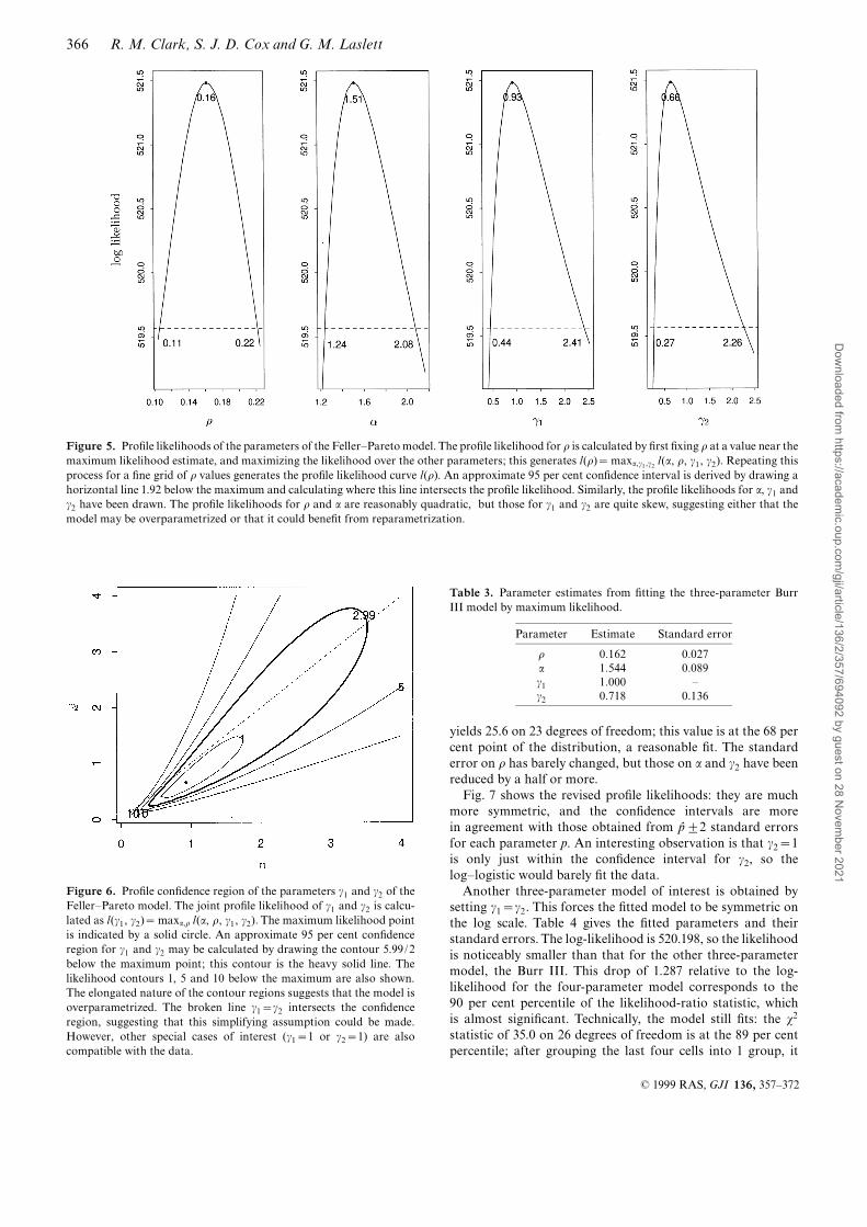
mended by Silverman (1986, p. 48)] of the log-transformedlengths is compared with the ¢tted Feller^Pareto model, alsotransformed to the log scale. The kernel density estimate makesno speci¢c allowance for truncation, but nonetheless the ¢tseems excellent for practical purposes, despite the s2 test. Thecomparison is also made on the original scale, to emphasizethe extreme skewness of the distribution of fault lengths. The¢tted and kernel density estimates overplot on the originalscale. The estimate of the density function f (x) on the originalscale is obtained by fê (x)~gª ( log x)/x, where gª is the kerneldensity estimate of the log-transformed data. This overcomesproblems with estimating a long-tailed distribution directly.Fig. 5 shows the pro¢le likelihoods of the four parameters

(o, a, c1, c2). For example, the pro¢le likelihood of o is com-puted, for each value of o, by maximizing the log-likelihoodwith respect to the remaining three parameters. Approximate95 per cent con¢dence limits for each parameter can be reado¡ the pro¢les by drawing a line 1.92 below the maximum ofthe log-likelihood, as shown. This is equivalent to repeatedapplication of the generalized likelihood-ratio test (e.g. Rice1987, p. 278); note that 1.92 is half the 95 per cent point of s2 on1 degree of freedom. These con¢dence limits seem rather wide,and for a, c1 and c2, they are skew, suggesting that the modelmight be overparametrized. Nevertheless, the case c1??seems to be excluded, suggesting that the Weibull, gamma andlognormal models would not ¢t. However, the log^logistic,

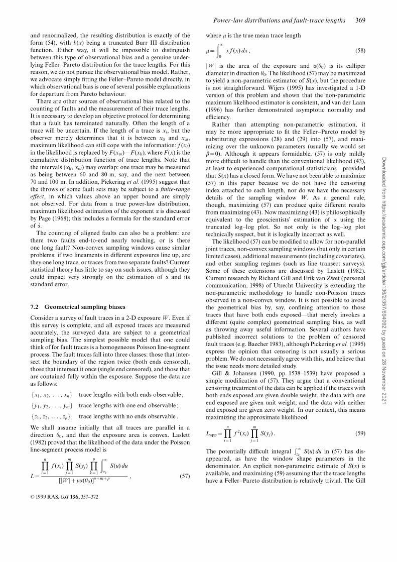
Burr III and Burr XII models are distinct possibilities, sincethe con¢dence intervals for c1 and c2 both include 1.Fig. 6 shows contours of the likelihood surface maximized

over o and a for various values of c1 and c2. An approximate 95per cent con¢dence region for c1 and c2 is outlined by a heavyline; this is the contour line 2.99 below the maximum of thelog-likelihood, the location of which is indicated by a solidcircle. Other contour lines are also shown, indicating theshape of the log-likelihood surface. If the model was correctlyparametrized, we would expect the solid circle to be roughly inthe middle of some elliptical contours. The elongated nature ofthe con¢dence region strengthens our suspicion that the modelmight be overparametrized, or, at the very least, that themodel should be reparametrized. A broken line indicates wherec1~c2; in this case, the distribution is symmetric on the logscale. We examine this possibility later.At this stage, we could declare ourselves happy with the

modelling, but it seems preferable to try some three-parametermodels.The four-parameter ¢t suggests that ¢xing c1~1 would not

degrade the ¢t much. This, in any case, corresponds to thepopular Burr III model. Table 3 lists the parameter estimatesand their standard errors when c1~1. The log-likelihood isnow 521.467, only 0.018 smaller than the four-parameter case,so the model ¢ts almost as well in likelihood terms. The s2

statistic is now 34.3 on 26 degrees of freedom, which is at the 87per cent point of the distribution. Grouping the last four cells

Figure 3. Survival function of the data and ¢tted truncated Feller^Pareto model. The log empirical survival function of the NE-strikingnormal faults is plotted as solid points against the log trace length(logx). The observational cut-o¡ is x0~0:01 km (log x0&{4:6). Thefour-parameter Feller^Pareto model ¢tted by maximum likelihood isshown as a solid line; for values of log x less than {1, the points andthe line overplot, indicating a well-¢tting model. The classical Paretomodel (broken line) is represented by two straight lines intersecting atj0: one has slope 0, and the other slope {aª ~{1:512. The ¢ttedFeller^Pareto model is asymptotic towards (i.e. becomes closer to) thebroken line as logx increases.

Figure 4. Density estimates of NE-striking normal fault data and the¢tted model. In the ¢rst panel the kernel density estimate of thelog trace-length data is plotted as a solid curve, and the ¢tted densityfrom the four-parameter truncated Feller^Pareto model is shown as abroken line. The agreement appears to be excellent. In the secondpanel, the densities are plotted on the original scaleöin this case thereis no visible di¡erence between the curves.

ß 1999 RAS,GJI 136, 357^372


ownloaded from



ber 2021

yields 25.6 on 23 degrees of freedom; this value is at the 68 percent point of the distribution, a reasonable ¢t. The standarderror on o has barely changed, but those on a and c2 have beenreduced by a half or more.Fig. 7 shows the revised pro¢le likelihoods: they are much

more symmetric, and the con¢dence intervals are morein agreement with those obtained from pª +2 standard errorsfor each parameter p. An interesting observation is that c2~1is only just within the con¢dence interval for c2, so thelog^logistic would barely ¢t the data.Another three-parameter model of interest is obtained by

setting c1~c2. This forces the ¢tted model to be symmetric onthe log scale. Table 4 gives the ¢tted parameters and theirstandard errors. The log-likelihood is 520.198, so the likelihoodis noticeably smaller than that for the other three-parametermodel, the Burr III. This drop of 1.287 relative to the log-likelihood for the four-parameter model corresponds to the90 per cent percentile of the likelihood-ratio statistic, whichis almost signi¢cant. Technically, the model still ¢ts: the s2

statistic of 35.0 on 26 degrees of freedom is at the 89 per centpercentile; after grouping the last four cells into 1 group, it

Figure 5. Pro¢le likelihoods of the parameters of the Feller^Pareto model. The pro¢le likelihood for o is calculated by ¢rst ¢xing o at a value near themaximum likelihood estimate, and maximizing the likelihood over the other parameters; this generates l(o)~maxa,c1,c2 l(a, o, c1, c2): Repeating thisprocess for a ¢ne grid of o values generates the pro¢le likelihood curve l(o). An approximate 95 per cent con¢dence interval is derived by drawing ahorizontal line 1.92 below the maximum and calculating where this line intersects the pro¢le likelihood. Similarly, the pro¢le likelihoods for a, c1 andc2 have been drawn. The pro¢le likelihoods for o and a are reasonably quadratic, but those for c1 and c2 are quite skew, suggesting either that themodel may be overparametrized or that it could bene¢t from reparametrization.

Table 3. Parameter estimates from ¢tting the three-parameter BurrIII model by maximum likelihood.


o 0:162 0:027a 1:544 0:089c1 1:000 =

c2 0:718 0:136

Figure 6. Pro¢le con¢dence region of the parameters c1 and c2 of theFeller^Pareto model. The joint pro¢le likelihood of c1 and c2 is calcu-lated as l(c1, c2)~maxa,o l(a, o, c1, c2):The maximum likelihood pointis indicated by a solid circle. An approximate 95 per cent con¢denceregion for c1 and c2 may be calculated by drawing the contour 5.99/2below the maximum point; this contour is the heavy solid line. Thelikelihood contours 1, 5 and 10 below the maximum are also shown.The elongated nature of the contour regions suggests that the model isoverparametrized. The broken line c1~c2 intersects the con¢denceregion, suggesting that this simplifying assumption could be made.However, other special cases of interest (c1~1 or c2~1) are alsocompatible with the data.

ß 1999 RAS, GJI 136, 357^372


ownloaded from



ber 2021

is 27.0 on 23 degrees of freedom at the 74 per cent point.However, there are some peculiarities: the standard error of ohas suddenly declined to 4 per cent of its estimate; for the c1~1model, it is 16 per cent. The standard errors of a and c1~c2 aremuch larger than in the four-parameter ¢t! A strange trade-o¡has occurred between the standard errors of the parameters.The pro¢le likelihoods of a and c1 are quite skew (Fig. 8). Thec1~c2 model seems much less satisfactory than the Burr III.

Figure 7. Pro¢le likelihoods of parameters of the Burr III model (i.e. the Feller^Pareto model with c1~1). The near-quadratic pro¢les arecharacteristic of a well-parametrized well-¢tting model.

Table 4. Parameter estimates from ¢tting the Feller^Pareto modelwith c1~c2 by maximum likelihood.


o 0:119 0:005a 1:571 0:395c1 1:347 0:828c2 1:347 0:828

Figure 8. Pro¢le likelihoods of the parameters of the Feller^Pareto model with c1~c2. The skewed pro¢le of c1 suggests that the model is imperfect.

ß 1999 RAS,GJI 136, 357^372


ownloaded from



ber 2021

What is the reason for the poor performance of the c1~c2model? Almost certainly, it can be traced back to Kalb£eisch &Prentice's (1980) log^linear representation. Consider eq. (35),with b~0, a~c1d, and let c~c1~c2. Then their log^linearmodel can be written

logX~ logozca[ logG2{ logG1] (50)

~ logoz

��cpa

[��cp

( logG2{ logG1)] , (51)

where G2*!(c) and G1*!(c). In this representation,log o is a location parameter and 1/a is a scale para-meter. Now, particularly for large c, the random variable��

cp

(logG2{ logG1)*N(0, 2), so we e¡ectively have a two-parameter model on the log scale, with location para-meter logo and scale parameter

��cp

/a. This suggests areparametrization, in which a new parameter l~

��cp

/a isde¢ned; we would expect l to be estimated quite well, and cto be almost inestimable, or very poorly estimated. Thisreparametrization, although statistically advantageous, is oflittle interest to the geoscientist, whose prime interest is a.[A somewhat similar criticism may be levelled at theChampernowne (1952) three-parameter model.]With reference to the preceding argument, note that the

mean of logGi is the digamma function t(ci), and the varianceis t'(ci), the trigamma function, but it is readily provedthat t(k)~ log kzO(k{1) and that t'(k)~k{1zO(k{2).The standardized variate

��cip

( logGi{ log ci) converges tonormality very fast as ci??. When we consider di¡erenceslogG2{ logG1 for two independent standard gamma variableswith the same c, the convergence to normality is even faster,being poor for c~0:1, adequate for c~0:5, and excellent forc§1. Mathematically, the skewness of logG2{ logG1 is 0, butthe kurtosis is approximately 3z(c{0:5){1 for large c, sothe information on c is largely contained in the kurtosis, whichis converging fairly rapidly to 3, the value for the normaldistribution.What is the reason for the Burr III's superior performance?

Consider equation (35) again. The Burr III model can bewritten as

logX~ logoz1a[logG2{ logG1] , (52)

where G2*!(c2) and G1*!(1); that is, G1 has the exponentialdistribution. Now logG2{ logG1 has a skewed distribution,with the amount of skewness depending on c2, so the distri-bution of logG2{ logG1 contains information that willallow c2 to be estimated; mathematically, the skewness oflogG2{ logG1 is, for large c2,��

2p

(c2{1)��c2(c2{0:5)

p &��2p

1{34c2

� �, (53)

so the skewness contains some information on c2, as well as thekurtosis. Thus the parameter c2 should behave well, in whichcase so should the location- and scale-related parameters log oand 1/a, and o and a in turn.

7 EXTENSIONS, PHYSICAL MODELS ANDCAUTIONARY REMARKS

It is possible that, for some poorly understood physicalreasons, there is a true Pareto distribution of fault lengths, but

that the observed distribution is modi¢ed from this for variousreasons that may be predicted or even modelled. In this sectionwe discuss a number of the more straightforward possibilities.For these and other reasons, the analysis conducted in Section 6should be treated with caution.

7.1 Observational biases

The data probably include a number of observational biases.As explained in Section 4, the trace lengths are measuredaccording to a convention of the minimum acceptable throw.The `true' lengths are probably longer, but it is di¤cult tosay how important this e¡ect is. It is vaguely reminiscent ofunder-reporting of incomes, and attempts have been madeto adjust income distribution data for this e¡ect (Arnold1983, Section 5.8.4). Watterson et al. (1995) present empiricalevidence indicating that the distribution of fault-trace lengthsmay be strongly in£uenced by the minimum throw.In addition, no formal survey of fault traces was carried

out. The information is a concatenation of data accrued overyears of working the coal seams, and some faults may havebeen missed, for a variety of reasons. It seems obvious thatthe smaller faults would have been missed more often than thelonger ones. Indeed, we could have built the modelling pro-cedure around such an assumption: we could suppose that thedeparture from the Pareto model is due to a bias factor, forwhich we could postulate a model and then ¢t it to the data.Thus, if p(x)~(x/j){a a/x is the density of the classical

Pareto distribution, we could assume that the density ofobserved trace lengths is

f (x)~b(x)p(x)/K for x§j ;

0 otherwise ,

((54)

where b(x) is a factor accounting for the non-observationof smaller faults, so is non-negative, and monotonicallyincreases to 1 as x??. It may be interpreted as the probabilitythat a trace of length x will be included in the survey. ThedenominatorK~

�b(x)p(x) dx is a normalizing constant. Thus

in this model the true distribution of trace lengths is Pareto,and we observe non-Pareto behaviour in the surveyed distri-bution because some small trace lengths are not recorded. TheFeller^Pareto model with b~0 is almost of this form. If wewrite

b(x)~(x/o)d(c1zc2)

[1z(x/o)d](c1zc2), (55)

which increases monotonically to 1 as x increases, then it iseasy to show that the Feller^Pareto density (28) is

f (x)~b(x)p(x) , (56)

where the parameters in p(x) are a~c1 d and j~

o/[c1B(c1, c2)]1=a. This is not quite the same as (54), in that p(x)

is non-zero for x < j, but it is very similar. It transpires thatb(x) is the cumulative distribution function of the Burr IIIdistribution [set b(x)~1{S(x) in (21) with a replaced by d, andc2 by c1zc2], so for x§j we can interpret the Feller^Pareto asa standard Pareto distribution sampled with a Burr III biasfactor. For x§j, the density p(x) is reduced by the bias factorb(x), and hence

�?j b(x)p(x) dx < 1; in the Feller^Pareto model,

this loss is made up for by extending the density f (x)~b(x)p(x)back to 0. Alternatively, if the Feller^Pareto is truncated at j

ß 1999 RAS, GJI 136, 357^372


ownloaded from



ber 2021

and renormalized, the resulting distribution is exactly of theform (54), with b(x) being a truncated Burr III distributionfunction. Either way, it will be impossible to distinguishbetween this type of observational bias and a genuine under-lying Feller^Pareto distribution for the trace lengths. For thisreason, we do not pursue the observational bias model. Rather,we advocate simply ¢tting the Feller^Pareto model directly, inwhich observational bias is one of several possible explanationsfor departure from Pareto behaviour.There are other sources of observational bias related to the

counting of faults and the measurement of their trace lengths.It is necessary to develop an objective protocol for determiningthat a fault has terminated naturally. Often the length of atrace will be uncertain. If the length of a trace is xi, but theobserver merely determines that it is between xli and xui,maximum likelihood can still cope with the information: f (xi)in the likelihood is replaced by F (xui){F (xli), where F (x) is thecumulative distribution function of trace lengths. Note thatthe intervals (xli, xui) may overlap: one trace may be measuredas being between 60 and 80 m, say, and the next between70 and 100 m. In addition, Pickering et al. (1995) suggest thatthe throws of some fault sets may be subject to a ¢nite-rangee¡ect, in which values above an upper bound are simplynot observed. For data from a true power-law distribution,maximum likelihood estimation of the exponent a is discussedby Page (1968); this includes a formula for the standard errorof aª .The counting of aligned faults can also be a problem: are

there two faults end-to-end nearly touching, or is thereone long fault? Non-convex sampling windows cause similarproblems: if two lineaments in di¡erent exposures line up, arethey one long trace, or traces from two separate faults? Currentstatistical theory has little to say on such issues, although theycould impact very strongly on the estimation of a and itsstandard error.

7.2 Geometrical sampling biases

Consider a survey of fault traces in a 2-D exposure W . Even ifthis survey is complete, and all exposed traces are measuredaccurately, the surveyed data are subject to a geometricalsampling bias. The simplest possible model that one couldthink of for fault traces is a homogeneous Poisson line-segmentprocess. The fault traces fall into three classes: those that inter-sect the boundary of the region twice (both ends censored),those that intersect it once (single end censored), and those thatare contained fully within the exposure. Suppose the data areas follows:

fx1, x2, . . . , xng trace lengths with both ends observable ;

fy1, y2, . . . , ymg trace lengths with one end observable ;

fz1, z2, . . . , zpg trace lengths with no ends observable .

We shall assume initially that all traces are parallel in adirection h0, and that the exposure area is convex. Laslett(1982) proved that the likelihood of the data under the Poissonline-segment process model is

L~

Yni~1

f (xi)Ymj~1

S(yj)Ypk~1

�?zk

S(u) du

[jW jzka(h0)]nzmzp , (57)

where k is the true mean trace length

k~

�?0

x f (x) dx , (58)

jW j is the area of the exposure and a(h0) is its calliperdiameter in direction h0. The likelihood (57) may be maximizedto yield a non-parametric estimator of S(x), but the procedureis not straightforward. Wijers (1995) has investigated a 1-Dversion of this problem and shown that the non-parametricmaximum likelihood estimator is consistent, and van der Laan(1996) has further demonstrated asymptotic normality ande¤ciency.Rather than attempting non-parametric estimation, it

may be more appropriate to ¢t the Feller^Pareto model bysubstituting expressions (28) and (29) into (57), and maxi-mizing over the unknown parameters (usually we would setb~0). Although it appears formidable, (57) is only mildlymore di¤cult to handle than the conventional likelihood (43),at least to experienced computational statisticiansöprovidedthat S(x) has a closed form.We have not been able to maximize(57) in this paper because we do not have the censoringindex attached to each length, nor do we have the necessarydetails of the sampling window W. As a general rule,though, maximizing (57) can produce quite di¡erent resultsfrom maximizing (43). Now maximizing (43) is philosophicallyequivalent to the geoscientists' estimation of a using thetruncated log^log plot. So not only is the log^log plottechnically suspect, but it is logically incorrect as well.The likelihood (57) can be modi¢ed to allow for non-parallel

joint traces, non-convex sampling windows (but only in certainlimited cases), additional measurements (including covariates),and other sampling regimes (such as line transect surveys).Some of these extensions are discussed by Laslett (1982).Current research by Richard Gill and Erik van Zwet (personalcommunication, 1998) of Utrecht University is extending thenon-parametric methodology to handle non-Poisson tracesobserved in a non-convex window. It is not possible to avoidthe geometrical bias by, say, con¢ning attention to thosetraces that have both ends exposedöthat merely invokes adi¡erent (quite complex) geometrical sampling bias, as wellas throwing away useful information. Several authors havepublished incorrect solutions to the problem of censoredfault traces (e.g. Baecher 1983), although Pickering et al. (1995)express the opinion that censoring is not usually a seriousproblem.We do not necessarily agree with this, and believe thatthe issue needs more detailed study.Gill & Johansen (1990, pp. 1538^1539) have proposed a

simple modi¢cation of (57). They argue that a conventionalcensoring treatment of the data can be applied if the traces withboth ends exposed are given double weight, the data with oneend exposed are given unit weight, and the data with neitherend exposed are given zero weight. In our context, this meansmaximizing the approximate likelihood

Lapp~Yni~1

f 2(xi)Ymj~1

S(yj) . (59)

The potentially di¤cult integral�?zk

S(u) du in (57) has dis-appeared, as have the window shape parameters in thedenominator. An explicit non-parametric estimate of S(x) isavailable, and maximizing (59) assuming that the trace lengthshave a Feller^Pareto distribution is relatively trivial. The Gill

ß 1999 RAS,GJI 136, 357^372


ownloaded from



ber 2021

& Johansen approach may be justi¢ed by breaking the datainto two overlapping subsamples, those with `northern end-points' exposed, and those with `southern endpoints' exposed,and multiplying together the likelihoods for each subsample.This is not strictly legitimate, because the two likelihoods arenot independent, but their multiplication may be defendedon pragmatic grounds, in that the resulting estimator willstill be asymptotically consistent. The notion of giving doubleweight to `two-enders' may be traced back to Palmer (1948),who applied this method to the estimation of ¢bre-lengthdistribution in textiles. Gill & Johansen (1990) extended theidea to incorporate censoring due to edge e¡ects. Denby &Vardi (1985) proposed a similar approach in a slightly di¡erentcontext.

7.3 Spatial e¡ects

The faults in the exposure may exhibit a number of importantspatial patterns. The primary fault map of Watterson et al.(1995) indicates that the spatial density of all fault sets variesconsiderably, with clusters of faults in several places. Onewould expect the fault-trace length distribution to vary withthe spatial density and the overall nature of the faulting system.Since we were given only the lengths, not the locations, ofthe faults, we are unable to make any such adjustment for thespatial intensity.There is also the related problem of interactions between

faults. As mentioned in Section 4, this is not a major problemfor the NE-striking faults, but it is a potential problem in mostdata sets. There seem to have been few published attemptsto model interactions between faults, although Serra (1982,pp. 565^566) describes a `Boole^Poisson' model, which heattributes to Conrad.

7.4 Stereological e¡ects

Fault-trace lengths are obtained by measurements from eithera planar section or a line transect in, for example, a miningtunnel. Hence the sampling of fault traces is performed ineither a 2-D or a 1-D subspace of the 3-D space in which thefaults are embedded. The distribution of the observed fault-trace lengths will not be the same as that of the `true' lengths,and some correction must be made for this lower-dimensionalsampling.Such corrections for this so-called `stereological sampling'

have been considered by many authors (Wicksell 1925;Danielsson et al. 1988; Dress & Reiss 1992). Such formulaegenerally make simplifying assumptions about the randomprocess generating the faults, and the shape of the faults.Whilethese assumptions are unlikely to be correct in practice, theformulae nevertheless give an indication of the importance ofa proper consideration of stereological e¡ects.A recent result by Dress & Reiss (1992) is relevant to our

study.We assume that the faults are circular in shape, each witha random diameter R. Let U denote the length of the inter-section of such a fault with a planar section. The importantpoint is that U does not have the same probability distributionas R. Suppose that the centres of the faults are distributedrandomly in space and the density function of R is f (r).According to Kendall & Moran (1963, eq. 4.55) the density

function of U is then

h(u)~ukR

�?u

f (r)��r2{u2p dr , (60)

where kR is the mean diameter of a fault chosen at random.Although Kendall & Moran (1963) do not state it explicitly,(60) holds if the diameter R and orientation ' of the fault arestatistically independent, but the orientation distribution isotherwise arbitrary. Now suppose that f (r) is the classicalPareto density (14) with a > 1, in which case kR~aj/(a{1)exists. Dress & Reiss (1992, Theorem 2) show that

u�?u

(r2{u2){1=2 f (r) dr~a2B

1za2

,12

� ��uj

�{a

, u§j ,

(61)

where B is the beta function.In other words, the upper tail of the density of U is of Pareto

form, but with the shape parameter a decreased by 1; thus if thediameter distribution has Pareto index 2.5, say, the tracelengths will have Pareto index 1.5. Dress & Reiss (1992) showthat a similar result holds when R has an arbitrary density witha Pareto upper tail.For certain purposes in structural geology, for example the

computation of total geological strain (Scholz & Cowie 1990),it is the distribution of R, notU , that matters. Danielsson et al.(1988) show in principle how to recover the distribution of Rfrom the observed distribution of U.

7.5 Mixtures of distributions

An alternative to generalized Pareto distributions is to ¢tmixtures of power-law models. If a single power-law distri-bution does not ¢t the data, the population might be assumedto be the union of two or more independent subpopulations.Thus, if f1(x) and f2(x) are classical power-law modelswith parameters (j1, a1) and (j2, a2), we might adopt a two-component mixture f (x)~p f1(x)z(1{p) f2(x) model for thedata, where the mixing proportion p is a parameter takingvalues between 0 and 1. Such a model has ¢ve unknown para-meters to be estimated: (p, j1, a1, j2, a2). A three-componentmixture model has eight unknown parameters. One potentialtrouble with this hierarchy of models is that the number ofparameters jumps by 3 each time: 2, 5, 8 . . . . For a particulardata set, one might ¢nd that a two-parameter model isunderparametrized, whereas the ¢ve-parameter model isoverparametrized. Consequently, we recommend that mixturesonly be ¢tted if there are compelling geological reasons for suchmodels. Even so, for technical reasons (numerical stability),one would be better advised to ¢t ¢nite mixtures of log^logisticor Burr III models than power-law models themselves, sosubmodels within the Feller^Pareto class are still useful.

8 CONCLUDING REMARKS

8.1 Results for South Yorkshire fault data

Our analyses show that several of the available Pareto-typemodels give a good ¢t to the fault-trace-length data from the1034 NE-striking normal faults. The Burr III distribution inparticular is a well-parametrized closely ¢tting model, andits parameters have quite a nice statistical interpretation, as

ß 1999 RAS, GJI 136, 357^372


ownloaded from



ber 2021

location, scale and skewness parameters in a log^linear model(see 36 and 53). Furthermore, the scale parameter p is thereciprocal of the Pareto index a.Our estimate of a from the Burr III model is 1.54 with an

approximate 95 per cent con¢dence interval of (1.38, 1.73).Wealso ¢tted a modi¢ed version of the Champernowne (1952)model, for which the estimates were almost identical: aª is1.53, with 95 per cent con¢dence interval for a of (1.37, 1.71)(Clark & Laslett 1995). These estimates may be compared withWalsh's visual estimate `ca: 1.2' (personal communication,1995) and Watterson et al.'s (1995) estimate of 1:36+0:06 forthis set (see their Table 3). It should be noted that Walsh &Watterson et al. (1995) are not quite estimating the samequantity as we are: our a is the asymptotic slope of the logS(x)versus log x curve, whereas they are estimating the averageslope or tangential slope of this curve at large values of x. Thetangential slope at x is

a1(x)~{d logS(x)d log x

~x f (x)S(x)

. (62)

For example, for the Burr III, we might choose x~1:0 km(i.e. log x~0) from an inspection of Fig. 3. Then

aª 1(1)~1:0|0:0604

0:0412~1:47 . (63)

This estimate does not di¡er very much fromWatterson et al.'s(1995) estimate of 1:36+0:06. It is important to decide whichparameter, the true Pareto index a or the approximation a1,should be used in strain calculations.

8.2 General conclusions

(1) Maximum likelihood rather than least squares should beused to estimate the exponent a of the classical power-law orPareto distribution (4). When the scale parameter j is known,the modi¢ed maximum likelihood estimator (7) gives theminimum variance unbiased estimator (MVUE) of a, withexact con¢dence limits given by (8). In contrast, the least-squares estimators are both biased and more variable thanthe MVUE, while their estimated standard errors are an orderof magnitude too small (a factor between 7 and 30 in oursimulation study).(2) The Feller^Pareto distribution (28) is an attractive class

of models which show power-law behaviour for large x. Thepower-law exponent is a~c1 d in our notation (27); if possiblea should replace d in the parameter set when the model isbeing ¢tted to data. Many standard statistical models arespecial cases of the Feller^Pareto class, especially if limitingforms are included. Some of the models within this class arepoorly parametrized or overparametrized, but in Table 5 werecommend one particular hierarchy of models as of primaryinterest, other things being equal. The Burr III could bereplaced by the Burr XII, although there may be problems withestimating a, because then c1=1. We do not recommendreplacing the Burr III model with the Feller^Pareto with

c1~c2:c, because then the third parameter c representskurtosis on the log scale, rather than skewness.The hierarchy of models in Table 5 adds one statistically

meaningful parameter at a time, so the model ¢tting may be¢ne-tuned to the data. This is a considerable advantage overmixtures discussed in Section 7.5, where including an extracomponent adds three more parameters to the model.(3) The parameters in these models can be readily estimated

by maximum likelihood using a suitable optimization routine,such as the Nelder^Mead algorithm. Standard errors maybe computed by inverting the observed information matrix.Alternatively, con¢dence limits may be read o¡ the pro¢lelikelihood function.(4) The three Feller^Pareto models listed in Table 5 all

behave like a power-law distribution for large x. These modelsmay contain nuisance parameters (here, parameters other thanj and a), which are needed to ¢t the distribution, althoughthey are not of primary interest. Such nuisance parametersmay be interpreted as de¢ning an adjustment for the possibleunder-reporting of small faults (see 54 and 55).(5) Any estimates derived from ¢tting Feller^Pareto models

are subject to the limitations of the data, such as observationalbiases, geometrical sampling biases and the like, as discussedin Section 7. Some of these biases can be allowed for, bymodifying the likelihood function, but only if the trace-lengthdata are recorded more fully.(6) A major objective of this paper is to encourage

practitioners to record their trace-length data in su¤cientdetail. We suggest the following format for fault tracesintersecting, say, a horizontal exposure: for each trace, record

(e1, n1, d1) (e2, n2, d2) , (64)

where (e1, n1) is the easting and northing of the ¢rst observedextremity of the fault trace, and d1 � 0 if it terminatesnaturally, and d1~1 if it is censored (i.e. truncates against theedge of the exposure),and similarly for the second extremity.Intermediate coordinates will be required if the fault trace isnot straight. This method of recording will enable the dataanalyst to convert the data into the form required for thelikelihood (57) or (59), and also to test if such an analysis isappropriate.Overall, this paper demonstrates that one of the main

issues being discussed in the geophysical literature, namelyhow to account for departure from Pareto behaviour in model¢tting, may be addressed quite easily using standard statisticalmethodology. However, there are other more practical pro-blems such as various forms of sampling bias, stereologicale¡ects and spatial structure that current statistical method-ology is only beginning to address, and these are possibly justas important, if not more important, than departures fromPareto behaviour.

ACKNOWLEDGMENTS

We would like to thank John Walsh and the Fault AnalysisGroup of Liverpool University for kindly supplying the dataset used in this study. The study was partly supported by theAustralian Research Council through grant A39031709 toSJDC. This paper is published with the permission of theDirector, AGCRC. We also thank the referee whose helpfulcomments led to several improvements in the presentation ofour results.

Table 5. Hierarchy of useful submodels of the Feller^Pareto class.

Model Fixed parameters Number of free parameters

Feller=Pareto b~0 4Burr III b~0, c1~1 3Log=logistic b~0, c1~1, c2~1 2

ß 1999 RAS,GJI 136, 357^372


ownloaded from



ber 2021

REFERENCES

Agterberg, F.P., 1995. Power-law versus lognormal models in mineralexploration, in Proc. 3rd Canadian Conference on ComputerApplications in the Mineral Industry, pp. 17^26, McGill University,Department of Mining and Metallurgical Engineering, Montreal.

Aki, K., 1965. Maximum likelihood estimate of b in the formulalogN~a{bM and its con¢dence limits, Bull. Earthq. Res. Inst., 43,237^238.

Arnold, B.C., 1983. Pareto Distributions, International CooperativePublishing House, Fairland, MD.

Baecher, G.B., 1983. Statistical analysis of rock mass fracturing, J. Int.Assoc. math. Geol., 15, 329^348.

Baxter, M.A., 1980. Minimum variance unbiased estimation of theparameters of the Pareto distribution, Metrika, 27, 133^138.

Burr, I.W., 1942. Cumulative frequency functions,Ann. math. Stat., 13,215^232.

Champernowne, D.G., 1952. The graduation of income distributions,Econometrica, 20, 591^615.

Clark, R.M. & Cox, S.J.D., 1996. A modern regression approachto determining fault displacement-length scaling relationships,J. struct. Geol., 18, 147^152.

Clark, R.M. & Laslett, G.M., 1995. Statistical analysis of faultlength distributions using generalized Pareto models, CSIRO DMSTechnical Report, DMS-E95/59.

Dagum, C., 1977. A new model of personal income distribution:speci¢cation and estimation, Economie Appliquee, 30, 413^436.

Danielsson, H., Andersson, J. & Sundberg, R., 1988. Estimationof fracture size and number distributions from observations inplanar sections or tunnels, Research Report, No. 150, Institute ofActuarial Mathematics and Mathematical Statistics, Universityof Stockholm.

Davis, H.T., 1941. The Analysis of Economic Time Series, PrincipiaPress, Bloomington, IN.

Davy, P., 1993. On the frequency-length distribution of the SanAndreas fault system, J. geophys. Res., 98, 12141^12151.

Denby, L. & Vardi, Y., 1985. A short-cut method for estimation ofrenewal processes, Technometrics, 27, 361^373.

Dress, H. & Reiss, R.-D., 1992. Tail behaviour in Wicksell'scorpuscle problem, in Probability and Applications, pp. 205^220,eds Galambos, J. & Katai, I., Kluwer, Dordrecht.

Dubey, S.D., 1968. A compound Weibull distribution, Naval ResearchLogistics Quarterly, 15, 179^188.

Feller, W., 1971. An Introduction to Probability Theory and itsApplications,Vol. 2, 2nd edn,Wiley, New York.

Fisk, P.R., 1961. The graduation of income distributions,Econometrica, 29, 171^185.

Fitton, N.C. & Cox, S.J.D., 1995. Linear feature extraction in geo-scienti¢c data, in Proc. 3rd Biennial Conference of the AustralianPattern Recognition Society. Digital Image Computing: Techniquesand Applications, pp. 104^109, eds Maeder, A. & Lovell, B.,Brisbane.

Gill, R.D. & Johansen, S., 1990. A survey of product-integrationwith a view toward application in survival analysis, Ann. Stat., 18,1501^1555.

Isles, D.J. & Cooke, A.C., 1990. Spatial associations between post-cratonisation dykes and gold deposits in the Yilgarn Block,WesternAustralia, inMa¢c Dykes and Emplacement Mechanisms, Proc. 2ndInt. Dyke Conference, Adelaide, 12^16 September, pp. 157^162, edsParker, A.J., Rickwood, P.C. & Tucker, D.H., Balkema, Rotterdam.

Johnson, N.L. & Kotz, S., 1970. Continuous UnivariateDistributionsöI, Houghton Mi¥in, New York.

Johnson, N.L. & Leone, F.C., 1964. Statistics and Experimental Designin Engineering and the Physical Sciences Î, Wiley, New York.Kalb£eisch, J.D. & Prentice, R.L., 1980. The Statistical Analysis ofFailure Time Data,Wiley, New York.

Kendall, M.G. & Moran, P.A.P., 1963. Geometrical Probability,Gri¤n, London.

Laslett, G.M., 1982. Censoring and edge e¡ects in areal and linetransect sampling of rock joint traces, J. Int. Assoc. math. Geol., 14,125^140.

Majumder, K.L. & Bhattacharjee, G.P., 1973. Algorithm AS 63:the incomplete beta integral, Appl. Stat., 22, 409^411.

Nelder, J.A. & Mead, R., 1965. A simplex method for functionminimization, Computer Journal, 7, 308^313.

Pacheco, J.F., Scholz, C.H. & Sykes, L.R., 1992. Changes in frequency-size relationship from small to large earthquakes, Nature, 355,71^73.

Page, R., 1968. Aftershocks and microaftershocks of the great Alaskaearthquake of 1964, Bull. seism. Soc. Am., 58, 1131^1168.

Palmer, R.C., 1948. The dye sampling method of measuring ¢brelength distribution, J. Textile Inst., 39, T8^T22.

Pareto, V., 1897. Cours d'economie politique, Vol. II, F. Rouge,Lausanne.

Patil, G.P., Boswell, M.T. & Ratnaparkhi, M.V., 1984. Dictionaryand Classi¢ed Bibliography of Statistical Distributions in Scienti¢cWork, Vol. 2, Continuous Univariate Models, InternationalCooperative Publishing House, Fairland, MD.

Pickering, G., Bull, J.M. & Sanderson, D.J., 1995. Sampling power-lawdistributions, Tectonophysics, 248, 1^20.

Rice, J.A., 1987. Mathematical Statistics and Data Analysis,Wadsworth, California.

Rutherford, R.S.G., 1955. Income distributions: a new model,Econometrica, 23, 277^294.

Scholz, C.H., 1995. Fractal transitions on geological surfaces, inFractals in the Earth Sciences, pp. 131^140, eds Barton, C.C. &La Pointe, P.R., Plenum, New York.

Scholz, C.H. & Cowie, P.A., 1990. Determination of total geologicstrain from faulting, Nature, 346, 837^839.

Scholz, C.H. & Mandelbrot, B.B., eds, 1989. Fractals in Geophysics,Birkhauser, Basel.

Serra, J., 1982. Image Analysis and Mathematical Morphology,Academic Press, London.

Silverman, B.W., 1986. Density Estimation for Statistics and DataAnalysis, Chapman & Hall, New York.

Singh, S.K. & Maddala, G.S., 1976. A function for size distribution ofincomes, Econometrica, 44, 963^970.

Turcotte, D.L. & Huang, J., 1995. Fractal distributions in geology,scale invariance and deterministic chaos, in Fractals in the EarthSciences, pp. 1^40, eds Barton, C.C. & La Pointe, P.R., Plenum,New York.

van der Laan, 1996. E¤ciency of the NPMLE in the line-segmentproblem, Scandinavian J. Stat., Theory and Applications, 23,527^550.

Watterson, J., Walsh, J.J., Gillespie, P.A. & Easton, S., 1995. Scalingsystematics of fault sizes on a large scale range fault map, FaultAnalysis Group Report, Department of Earth Sciences, Universityof Liverpool.

Westaway, R., 1994. Quantitative analysis of populations of smallfaults, J. struct. Geol., 16, 1259^1273.

Wicksell, S.D., 1925. The corpuscle problem, Biometrika, 17, 84^89.Wijers, B.J., 1995. Consistent non-parametric estimation for a

one-dimensional line segment process observed in an interval,Scandinavian J. Stat., 22, 335^360.

ß 1999 RAS, GJI 136, 357^372


ownloaded from



ber 2021

Documents

Generalizations of powerlaw distributions applicable to sampled