Generalising the Hardy–Littlewood method for primesicm2006.org › proceedings › Vol_II › contents › ICM_Vol_2_17.pdf · The Hardy–Littlewood method is a well-known technique

Generalising the Hardy–Littlewood method for primes

Ben Green∗

Abstract. The Hardy–Littlewood method is a well-known technique in analytic number theory.Among its spectacular applications are Vinogradov’s 1937 result that every sufficiently largeodd number is a sum of three primes, and a related result of Chowla and Van der Corput givingan asymptotic for the number of 3-term progressions of primes, all less than N . This articlesurveys recent developments of the author and T. Tao, in which the Hardy–Littlewood methodhas been generalised to obtain, for example, an asymptotic for the number of 4-term arithmeticprogressions of primes less than N .

Mathematics Subject Classification (2000). 11B25.

Keywords. Hardy–Littlewood method, prime numbers, arithmetic progressions, nilsequences.

1. Introduction

Godfrey Harold Hardy and John Edensor Littlewood wrote, in the 1920s, a famousseries of papers Some problems of “partitio numerorum”. In these papers, whosecontent is elegantly surveyed byVaughan [31], they developed techniques having theirgenesis in work of Hardy and Ramanujan on the partition function [18] to well-knownquestions in additive number theory such as Waring’s problem and the Goldbachproblem.

Papers III and V in the series, [16], [17], were devoted to the sequence of primes.In particular it was established on the assumption of the Generalised Riemann Hy-pothesis that every sufficiently large odd number is the sum of three primes. In 1937Vinogradov [33] made a further substantial advance by removing the need for anyunproved hypothesis.

The Hardy–Littlewood–Vinogradov method may be applied to give an asymptoticcount for the number of solutions in primes pi to any fixed linear equation

a1p1 + · · · + atpt = b

in, say, the box p1, . . . , pt � N , provided that at least 3 of the ai are non-zero.This includes the three-primes result, and also the result that there are infinitely many

∗This research was partially conducted during the period the author served as a Clay Research Fellow. Hewould like to express his sincere gratitude to the Clay Institute, and also to the Massachusetts Institute ofTechnology, where he was a Visiting Professor for the academic year 2005-06.

Proceedings of the International Congressof Mathematicians, Madrid, Spain, 2006© 2006 European Mathematical Society

374 Ben Green

triples of primes p1 < p2 < p3 in arithmetic progression, due to Chowla [4] and vander Corput [29].

More generally the Hardy–Littlewood method may also be used to investigatesystems such as Ap = b, where A is an s × t matrix with integer entries and,potentially, s > 1. A natural example of such a system is given by the (k − 2) × k

matrix

A :=

⎛⎜⎜⎝1 −2 1 0 . . . 0 0 00 1 −2 1 . . . 0 0 0

. . .

0 0 0 0 . . . 1 −2 1

⎞⎟⎟⎠ , (1)

in which case a solution to Ap = 0 is just a k-term arithmetic progression of primes.Here, unfortunately, the Hardy–Littlewood method falters in that it generally re-

quires t � 2s + 1. In particular it cannot be used to handle progressions of lengthfour or longer. There are certain special systems with fewer variables which canbe handled. In this context we take the opportunity to mention a beautiful result ofBalog [2], where it is shown that for any m there are distinct primes p1 < · · · < pm

such that each number 12 (pi + pj ) is also prime, or in other words that the system

p1 + p2 = 2p12

... (2)

pm−1 + pm = 2pm−1,m

has a solution in primes p1, . . . , pm, p12, . . . , pm−1,m. There is also a result ofHeath-Brown [19], in which it is established that there are infinitely many four-termprogressions in which three members are prime and the fourth is either a prime or aproduct of two primes.

The survey of Kumchev and Tolev [25] gives a detailed account of applications ofthe Hardy–Littlewood method to additive prime number theory.

The aim of this survey is to give an overview of recent joint work with TerenceTao [13], [14], [15]. Our aim, which has been partially successful, is to extend theHardy–Littlewood method so that it is capable of handling a more-or-less arbitrarysystem Ap = b, subject to the proviso that we do not expect to be able to handle anysystem which secretly encodes a “binary” problem such as Goldbach or Twin Primes.

This is a large and somewhat technical body of work. Perhaps my main aim hereis to give a guide to our work so far, pointing out ways in which the various papersfit together, and future directions we plan to take. A subsidiary aim is to focus as faras possible on key concepts, rather than on details. Of course, one would normallyaim to do this in a survey article. However in our case we expect that many of thesedetails will be substantially cleaned up in future incarnations of the theory, whilst thekey concepts ought to remain more-or-less as they are.

I will say rather little about our paper [12] establishing that there are arbitrarilylong arithmetic progressions of primes. Whilst there is considerable overlap between

Generalising the Hardy–Littlewood method for primes 375

that paper and the ideas we discuss here, those methods were somewhat “soft” whereasthe flavour of our more recent work is distinctly “hard”. We refer the reader to thesurvey of Tao in Volume II of these Proceedings, and also to the surveys [11], [23],[27], [28].

To conclude this introduction let me remark that the reader should not be underthe impression that the Hardy–Littlewood method only applies to linear equationsin primes, or even that this is the most popular application of the method. Therehas, for example, been a huge amount done on the circle of questions surroundingWaring’s problem. For a survey see [32]. More generally there are many spectacularresults where variants of the method are used to locate integer points on quite generalvarieties, provided of course that there are sufficiently many variables. The readermay consult Wooley’s survey [34] for more information on this.

2. The Hardy–Littlewood heuristic

We have stated our interest in systems of linear equations in primes. While we arestill somewhat lacking in theoretical results, there are heuristics which predict whatanswers we should expect in more-or-less any situation.

It is natural, when working with primes, to introduce the von Mangoldt function� : N → R�0, defined by

�(n) :={

log p if n = pk is a prime power,

0 otherwise.

The prime powers with k � 2 make a negligible contribution to any additive expressioninvolving �. Thus, for example, the prime number theorem is equivalent to thestatement that

En�N�(n) = 1 + o(1).

Here we have used the very convenient notation of expectation from probability theory,setting Ex∈X := |X|−1 ∑

x∈X for any set X. The notation o(1) refers to a quantitywhich tends to zero as N → ∞.

We now discuss a version of the Hardy–Littlewood heuristic for systems of linearequations in primes. Here, and for the rest of the article, we restrict attention tohomogeneous systems for simplicity of exposition.

Conjecture 2.1 (Hardy–Littlewood). Let A be a fixed s×t matrix with integer entriesand such that there is at least one non-zero solution to Ax = 0 with x1, . . . , xt � 0.Then

Ex1,...,xt�NAx=0

�(x1) . . . �(xt ) = S(A)(1 + o(1))

376 Ben Green

as N → ∞, where the singular series S(A) is equal to a product of local factors∏p αp, where

αp :=(

p

p − 1

)t

limM→∞

P(Ax = 0, (x1, p) = · · · = (xt , p) = 1|x ∈ [−M, M]t )P(Ax = 0|x ∈ [−M, M]t ) .

The singular series reflects “local obstructions” to having solutions to Ax = 0in primes; in the simple example A = (

1 9 −27), where the associated equation

p1+9p2−27p3 = 0 has no solutions, one has α3 = 0. A more elegant formulation ofthe conjecture would include a “local obstruction at ∞” α∞, in exchange for removingthe hypothesis on A.

Chowla and van der Corput’s results concerning three-term progressions of primesconfirm the prediction Conjecture 2.1 for the matrix A = (

1 −2 1). From this it

is easy to derive an asymptotic for the number of triples (p1, p2, p3), p1 < p2 <

p3 � N , of primes in arithmetic progression.

Theorem 2.2 (Chowla, van der Corput, [4], [29]). The number of triples of primes(p1, p2, p3), p1 < p2 < p3 � N , in arithmetic progression is

S3N2 log−3 N(1 + o(1)),

where

S3 := 1

2

∏p�3

(1 − 1

(p − 1)2

)≈ 0.3301.

The singular series S3 is equal to 14S(A), where A = (

1 −2 1), and is also half

the twin prime constant.Certain systems Ap = b should be thought of as very difficult indeed, since their

understanding implies an understanding of a binary problem such as the Goldbach ortwin prime problem. If A has the property that every non-zero vector in its row span(over Q) has at least three non-zero entries then there is no such reason to believe thatit should be fantastically hard to solve.

Definition 2.3 (Non-degenerate systems). Suppose that s, t are positive integers witht � s + 2. We say that an s × t matrix A with integer entries is non-degenerate ifit has rank s, and if every non-zero vector in its row span (over Q) has at least threenon-zero entries.

The reader may care to check that the system (1) defining a progression of length k

is non-degenerate.Our eventual goal is to prove Conjecture 2.1 for all non-degenerate systems. This

goal may be subdivided into subgoals according to the value of s.

Conjecture 2.4 (Asymptotics for s simultaneous equations). Fix a value of s � 1and suppose that t � s + 2 and that A is a non-degenerate s × t matrix. ThenConjecture 2.1 holds for the system Ap = 0.


One can also formulate an appropriate conjecture for non-homogeneous systemsAp = b, and one would not expect to encounter significant extra difficulties in provingit. One might also try to count prime solutions to Ap = 0 in which the primes pi aresubject to different constraints pi � Ni , or perhaps are constrained to lie in a fixedarithmetic progression pi ≡ ai (mod qi). One would expect all of these extensionsto be relatively straightforward.

The classical Hardy–Littlewood method can handle the case s = 1 of Conjec-ture 2.4. Our new developments have led to a solution of the case s = 2. In particularwe can obtain an asymptotic for the number of 4-term arithmetic progressions ofprimes, all less than N :

Theorem 2.5 (Green–Tao [15]). The number of quadruples of primes (p1, p2, p3, p4),p1 < p2 < p3 < p4 � N , in arithmetic progression is

S4N2 log−4 N(1 + o(1)),

where

S4 := 3

4

∏p�5

(1 − 3p − 1

(p − 1)3

)≈ 0.4764.

3. The Hardy–Littlewood method for primes

The aim of this section is to describe the Hardy–Littlewood method as it wouldnormally be applied to linear equations in primes. We will sketch the proof of The-orem 2.2, the asymptotic for the number of 3-term progressions of primes. This isequivalent to the s = 1 case of Conjecture 2.4 for the specific matrix A = (

1 −2 1).

Very similar means may be used to handle the general case s = 1 of that conjecture.The Hardy–Littlewood method is, first and foremost, a method of harmonic anal-

ysis. The primes are studied by introducing the exponential sum (a kind of Fouriertransform)

S(θ) := En�N�(n)e(θn)

for θ ∈ R/Z, where e(α) := e2πiα . It is the appearance of the circle R/Z here whichgives the Hardy–Littlewood method its alternative name. Now it is easy to check that

Ex1,x2,x3�N�(x1)�(x2)�(x3)1x1−2x2+x3=0 =∫ 1

0S(θ)2S(−2θ) dθ.

whence

Ex1,x2,x3�Nx1−2x2+x3=0

�(x1)�(x2)�(x3) = (2N + O(1))

∫ 1

0S(θ)2S(−2θ) dθ. (3)

The method consists of gathering information about S(θ), and then using this formulato infer an asymptotic for the left-hand side.

378 Ben Green

The process of gathering information about S(θ) leads us to another key featureof the Hardy–Littlewood method: the realisation that one must split the set of θ intotwo classes, the major arcs M in which θ ≈ a/q for some small q and the minor arcsm := [0, 1) \ M. To see why, let us attempt some simple evaluations. First of all wenote that

S(0) := En�N�(n) = 1 + o(1),

this being equivalent to the prime number theorem. To evaluate S(1/2), observe thatalmost all of the support of � is on odd numbers n, for which e(n/2) = −1. Thus

S(1/2) := En�N�(n)e(n/2) = −1 + o(1).

The evaluation of S(1/3) is a little more subtle. Most of the support of � is on n

not divisible by 3, and for those n the character e(n/3) takes two values according asn ≡ 1(mod 3) or n ≡ 2 (mod 3). We have

S(1/3) = e(1/3)En�N1n≡1 (mod 3)�(n) + e(2/3)En�N1n≡2 (mod 3)�(n) + o(1)

= −1/2 + o(1),

this being a consequence of the fact that the primes are asymptotically equally dividedbetween the congruence classes 1(mod 3) and 2 (mod 3).

In similar fashion one can get an estimate for S(a/q) for small q, and indeed forS(a/q+η) for sufficiently small η, if one uses the prime number theorem in arithmeticprogressions. The set of such θ is called the major arcs and is denoted M. (The notionof “small q” might be q � logA N , for some fixed A. The notion of “small η” mightbe |η| � logA N/qN . The flexibility allowed here depends on what type of primenumber theorem along arithmetic progressions one is assuming. Unconditionally, thebest such theorem is due to Siegel and Walfisz and it is this theorem which leads tothese bounds on q and |η|.)

Suppose by contrast that θ /∈ M, that is to say θ is not close to a/q with q small.We say that θ ∈ m, the minor arcs. It is hard to imagine that in the sum

S(√

2 − 1) = En�N�(n)e(n√

2) (4)

the phases e(n√

2) could conspire with �(n) to prevent cancellation. It turns out thatindeed there is substantial cancellation in this sum. This was first proved by Vino-gradov, and nowadays it is most readily established using an identity of Vaughan [30],which allows one to decompose (4) into three further sums which are amenable toestimation. We will discuss a variant of this method in §5. For the particular valueθ = √

2 − 1, and for other highly irrational values, one can obtain an estimate ofthe shape |S(θ)| N−c for some c > 0, which is quite remarkable since applyingthe best-known error term in the prime number theorem only allows one to estimateS(0) with the much larger error O(exp(−Cε log3/5−ε N)). By defining parameterssuitably (that is by taking a suitable value of the constant A in the precise definition


of M), one can arrange that S(θ) is always very small indeed on the minor arcs m,say

supθ∈m

|S(θ)| log−10 N. (5)

Recall now the formula (3). Splitting the integral into that over M and that over m,we see from Parseval’s identity that∣∣∣∣ ∫

mS(θ)2S(−2θ) dθ

∣∣∣∣ � supθ∈m

|S(θ)|∫ 1

0|S(θ)|2 dθ log−9 N

N. (6)

Thus in the effort to establish Theorem 2.2 the contribution from the minor arcs m

may essentially be ignored. The proof of that theorem is now reduced to showing that∫M

S(θ)2S(−2θ) dθ = (1 + o(1))1

N

∏p�3

(1 − 1

(p − 1)2

).

Since one has asymptotic formulæ for S(θ) (and S(−2θ)) on M, this is essentiallyjust a computation, albeit not a particularly straightforward one.

It is instructive to look for the point in the above argument where we used the factthat A was non-degenerate, that is to say that our problem had at least three variables.Why can we not use the same ideas to solve the twin prime or Goldbach problems?The answer lies in the bound (6). In the twin prime problem we would be looking tobound ∣∣∣∣ ∫

θ∈m|S(θ)|2e(2θ)

∣∣∣∣,and the only obvious means of doing this is via an inequality of the form∣∣∣∣ ∫

θ∈m|S(θ)|2e(2θ)

∣∣∣∣ � supθ∈m

|S(θ)|c∫ 1

0|S(θ)|2−c dθ.

Now, however, Parseval’s identity does not permit one to place a bound on∫ 1

0|S(θ)|2−c dθ.

Indeed this whole endeavour is rather futile since heuristics predict that the minor arcsactually make a significant contribution to the asymptotic for twin primes.

An attempt to count 4-term progressions in primes via the circle method is besetby difficulties of a similar kind.

4. Exponential sums with Möbius

The presentation in the next two sections (and in our papers) is influenced by that inthe beautiful book of Iwaniec and Kowalski [21].

380 Ben Green

In the previous section we described what is more-or-less the standard approachto solving linear equations in primes using the Hardy–Littlewood method. In [21,Ch. 19] one may find a very elegant variant in which the Möbius function μ is madeto play a prominent rôle. As we saw above the behaviour of the exponential sum S(θ)

was a little complicated to describe, depending as it does on how close to a rational θ

is. By contrast the exponential sum

M(θ) := En�Nμ(n)e(θn)

has a very simple behaviour, as the following result of Davenport shows.

Proposition 4.1 (Davenport’s bound). We have the estimate

|M(θ)| A log−A N

uniformly in θ ∈ [0, 1) for any A > 0.

In fact on the GRH Baker and Harman [1] obtain the superior bound |M(θ)| N−3/4+ε. By analogy with results of Salem and Zygmund [26] concerning ran-dom trigonometric series one might guess that the truth is that supθ∈[0,1) |M(θ)| ∼c√

log N/N . This is far from known even on GRH; so far as I am aware no lowerbound of the form supθ∈[0,1) |M(θ)|√N → ∞ is known.

Although Davenport’s result is easy to describe its proof has the same ingredientsas used in the analysis of S(θ). One must again divide R/Z into major and minorarcs. On the major arcs one must once more use information equivalent to a primenumber theorem along arithmetic progressions, that is to say information on the zerosof L-functions L(s, χ) close to the line �s = 1. On the minor arcs one uses anappropriate version of Vaughan’s identity. One of the attractions of working withMöbius is that this identity takes a particularly simple form (see [21, Ch. 13] or [14]).

We offer a rough sketch of how Proposition 4.1 may be used as the main ingredientin a proof of Theorem 2.2, referring the reader to [21, Ch. 19] for the details. The keypoint is that one has the identity

�(n) =∑d|n

μ(d) log(n/d).

One splits the sum over d into the ranges d � N1/10 and d > N1/10 (say), obtaininga decomposition � = � + �. One has

S(θ) := En�N�(n)e(nθ) =∑

d�N1/10

log d∑

N1/10�k�N/d

μ(k)e(θkd),

from which it follows easily using Davenport’s bound that

S(θ) A log−A N (7)


uniformly in θ ∈ [0, 1).One may then write the expression

Ex1,x2,x3�Nx1−2x2+x3=0

�(x1)�(x2)�(x3)

as a sum of eight terms using the splitting � = � + �. The basic idea is now thatthe main term

∏p αp in Theorem 2.2 comes from the term with three copies of �,

whilst the other 7 terms (each of which contains at least one �) provide a negligiblecontribution in view of (7) and simple variants of the formula (3).

We have extolled the virtues of the Möbius function by pointing to the aestheticqualities of Davenport’s bound. A more persuasive argument for focussing on it isthe following basic metaprinciple of analytic number theory:

Principle (Möbius randomness law). The Möbius function is highly orthogonal toany “reasonable” bounded function f : N → C. That is to say

En�Nμ(n)f (n) = o(1),

and usually one would in fact expect

En�Nμ(n)f (n) N−1/2+ε. (8)

In the category “reasonable” in this context one would certainly include polynomi-als phases and other somewhat continuous objects, but one should exclude functions f

which are closely related to the primes (f = μ and f = �, for example, are clearlynot orthogonal to Möbius).

At a finer level than is relevant to our work, the Möbius randomness law is morereliable than other heuristics that one might formulate, for example concerning �.In [22] it is shown that

En�N�(n)λ(n)e(−2√

n) ∼ cN−1/4,

where λ(n) := n−11/2τ(n) is a normalised version of Ramanujan’s τ -function. Onecould hardly be called naïve for expecting square root cancellation here.

5. Proving the Möbius randomness law

In the last section we mentioned a principle, the Möbius randomness law, which isvery useful as a guiding principle in analytic number theory. Unfortunately it is notpossible to prove the strong version (8) of the principle in any case – even whenf (n) ≡ 1 it is equivalent to the Riemann hypothesis.

It is, however, possible to prove weaker estimates of the form

En�Nμ(n)f (n) A log−A N, (9)

382 Ben Green

for arbitrary A > 0, for a wide variety of functions f . Davenport’s bound is pre-cisely this result when f (n) = e(θn) (and, furthermore, this result is uniform in θ ).Similar statements are also known for polynomial phases and for Dirichlet characters(uniformly over all characters of a fixed conductor).

Now when it comes to proving an estimate of the form (9), one should think of therebeing two different classes of behaviour for f . In the first class are those f whichare in a vague sense multiplicative, or linear combinations of a few multiplicativefunctions. Then the behaviour of En�Nμ(n)f (n) can be intimately connected withthe zeros of L-functions. One has, for example, the formula

∞∑n=1

μ(n)χ(n)n−s = 1

L(s, χ)

for any fixed Dirichlet character χ . By the standard contour integration technique(Perron’s formula) of analytic number theory one sees that En�Nμ(n)χ(n) is smallprovided that L(s, χ) does not have zeros close to �s = 1. (In fact, as reported on[21, p. 124], there are complications caused by possible multiple zeros of L, and it isbetter to work first with the sum En�N�(n)χ(n) of χ over primes.)

The need to consider zeros of L-functions can also be felt when considering addi-tive characters e(an/q), for relatively small q. Indeed any Dirichlet character to themodulus q may be expressed as a linear combination of such characters. Converselyany additive character e(an/q) may be written as a linear combination of Dirichletcharacters to moduli dividing q by using Gauss sums. By applying Siegel’s theorem,which gives the best unconditional information concerning the location of zeros ofL(s, χ) near to �s = 1, one obtains for any A the estimate

En�Nμ(n)e(an/q) A log−A N,

uniformly for q � logA N . By partial summation the same estimate holds when a/q

is replaced by θ = a/q + η for suitably small η, that is to say for all θ which lie inthe set M of major arcs.

We turn now to a completely different technique for bounding En�Nμ(n)f (n).Remarkably this is at its most effective when the previous technique fails, that is tosay when f is somehow far from multiplicative.

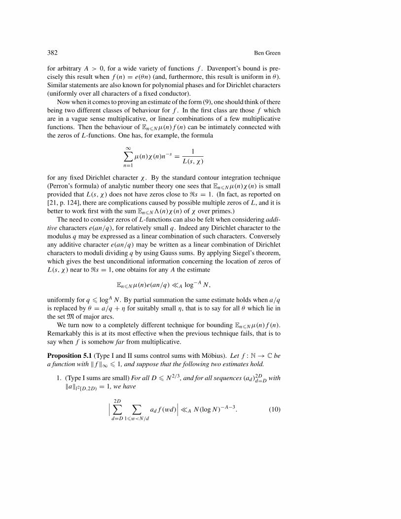
Proposition 5.1 (Type I and II sums control sums with Möbius). Let f : N → C bea function with ‖f ‖∞ � 1, and suppose that the following two estimates hold.

1. (Type I sums are small) For all D � N2/3, and for all sequences (ad)2Dd=D with

‖a‖l2[D,2D) = 1, we have

∣∣∣ 2D∑d=D

∑1�w<N/d

adf (wd)

∣∣∣ A N(log N)−A−3. (10)


2. (Type II sums are small) For all D, W , N1/3 � D � N2/3, N1/3 � W � N/D

and all choices of complex sequences (ad)2Dd=D, (bw)2W

w=W with ‖a‖l2[D,2D)

= ‖b‖l2[W,2W) = 1, we have

∣∣∣ 2D∑d=D

∑W�w�2W

adbwf (wd)

∣∣∣ A N(log N)−A−5. (11)

ThenEn�Nμ(n)f (n) A log−A N. (12)

The reader may find a proof of this statement in [14, Ch. 6]. It is proved bydecomposing the Möbius function into two parts using an identity of Vaughan [30].When one multiplies by f (n) and sums, one of these parts leads to Type I sums andthe other to Type II sums. Note that there is considerable flexibility in arranging theranges of D in which Type I and II estimates are required, but it is not important tohave such flexibility in our arguments.

The statement of Proposition 5.1 may look complicated. What has been achieved,however, is the elimination of μ. Strictly speaking, one actually only needs Type Iand II estimates for some rather specific choices of coefficients ad, bw whose definitioninvolves μ. The important realisation is that it is best to forget about the precise formsof these coefficients, the general expressions (10) and (11) laying bare the importantunderlying information required of f .

Note that if f is close to multiplicative then there is no hope of obtaining enoughcancellation in Type II sums to make use of Proposition 5.1. If f is actually completelymultiplicative, for example, one may take ad = f (d) and bw = f (w) and there ismanifestly no cancellation at all in (11). If this is not the case, however, then veryoften it is possible to verify the bounds (10) and (11). An example of this is a linearphase e(θn) where θ lies in the minor arcs m, that is to say θ is not close to a/q with q

small. By verifying these two estimates for such θ , one has from (12) that Davenport’sbound holds when θ ∈ m. This completes the proof of Davenport’s bound, since themajor arcs M have already been handled using L-function technology.

To see how this is usually achieved in practice we refer the reader to [5, Ch. 24].There the reader will see that a key device is the Cauchy–Schwarz inequality, whichallows one to eliminate the arbitrary coefficients ad , bw.

In [14] there is also a discussion of this result. Although logically equivalent, thisdiscussion takes a point of view which turns out to be invaluable when dealing withmore complicated situations. Taking f (n) = e(θn) in Proposition 5.1, we supposethat either (10) or (11) does not hold, that is to say that either a Type I or a Type II sumis large. We then deduce that θ must be close to a rational with small denominator,that is to say θ must be major arc. This inverse approach to bounding sums withMöbius means that there is no need to make an a priori definition of what a “major”or “minor” object is. In situations to be discussed later this helps enormously.

384 Ben Green

6. The insufficiency of harmonic analysis

What did we mean when we stated that the Hardy–Littlewood method was a methodof harmonic analysis? In §3 we saw that there is a formula, (3), which expresses thenumber of 3-term progressions in a set (such as the primes) in terms of the exponentialsum over that set. The following proposition is an easy consequence of a slightlygeneralised version of that formula:

Proposition 6.1. Suppose that f1, f2, f3 : [N] → [−1, 1] are three functions andthat

|Ex1,x2,x3x1−2x2+x3=0

f1(x1)f2(x2)f3(x3)| � δ.

Then for any i = 1, 2, 3 we have

supθ∈[0,1)

|En�Nfi(n)e(nθ)| � (1 + o(1))δ/2. (13)

We think of this as a statement the effect that the linear exponentials e(nθ) form acharacteristic system for the linear equation x1−2x2+x3 = 0. It follows immediatelyfrom Proposition 6.1 and Davenport’s bound that Möbius exhibits cancellation along3-term APs, in the sense that

Ex1,x2,x3x1−2x2+x3=0

μ(x1)μ(x2)μ(x3) A log−A N.

Proposition 6.1 is also useful for counting progressions in sets A ⊆ [N], in whichcontext one would take various of the fi to equal the balanced function fA := 1A −α

of A, where α := |A|/N . It is easy to deduce from Proposition 6.1 the followingvariant, which covers this situation.

Proposition 6.2. Suppose that A ⊆ [N ] is a set with |A| = αN and that

|Ex1,x2,x3x1−2x2+x3=0

1A(x1)1A(x2)1A(x3) − α3| � δ.

WritefA := 1A − α

for the balanced function of A. Then we have

supθ∈[0,1)

|En�NfA(n)e(nθ)| � (1 + o(1))δ/14. (14)

If a function f correlates with a linear exponential as in (13) or (14) then wesometimes say that f has linear bias.

In this section we give examples which show that the linear exponentials do notform a characteristic system for the pair of equations x1−2x2+x3 = x2−2x3+x4 = 0defining a four-term progression. These examples show, in a strong sense, that theHardy–Littlewood method in its traditional form cannot be used to study 4-term


progressions. An interesting feature of these two examples is that they were bothessentially discovered by Furstenberg and Weiss [6] in the context of ergodic theory.Much of our work is paralleled in, and in fact motivated by, the work of the ergodictheory community. See the lecture by Tao in Volume II of these proceedings, or theelegant surveys of Kra [23], [24] for more discussion and references. The exampleswere rediscovered, in the finite setting, by Gowers [8], [10] in his work on Szemerédi’stheorem.

Example 6.1 (Quadratic and generalised quadratic behaviour). Let α > 0 be a small,fixed, real number, and define the following sets. Let A1 be defined by

A1 := {x ∈ [N] : {x2√

2} ∈ [−α/2, α/2]}(here, {t} denotes the fractional part of t , and lies in (−1/2, 1/2]). Define also

A2 := {x ∈ [N ] : {x√2{x√

3}} ∈ [−α/2, α/2]}.Now it can be shown (not altogether straightforwardly) that |A1|, |A2| ≈ αN , and

furthermore thatsup

θ∈[0,1)

|En�NfA(n)e(nθ)| N−c

for i = 1, 2. Thus neither of the sets A1, A2 has linear bias in a rather strong sense. Ifthe analogue of Proposition 6.2 were true for four term progressions, then, one wouldexpect both A1 and A2 to have approximately α4N2/6 four-term progressions.

The set A1, however, has considerably more 4-term APs that this in view of theidentity

x2 − 3(x + d)2 + 3(x + 2d)3 − (x + 3d)2 = 0. (15)

This means that if x, x + d, x + 2d ∈ A1 then

{(x + 3d)2√

2} ∈ [−7α/2, 7α/2],which would suggest that x + 3d ∈ A1 with probability � 1. In fact one can showusing harmonic analysis that (15) is the only relevant constraint in the sense that

P(x + 3d ∈ A1|x, x + d, x + 2d ∈ A1)

≈ P(y1 − 3y2 + 3y3 ∈ [−1, 1]|y1, y2, y3 ∈ [−1, 1]) = 8/27.

The number of 3-term progressions in A1 is ≈ α3N/4, and so it follows that thenumber of 4-term progressions in A1 is ≈ 2α3/27.

The analysis of A2 is rather more complicated. However one may check that if|{x√

3}|, |{d√3}| � 1/10 and if |{y√

2{y√3}}| � α/10 for y = x, x + d, x + 2d,

then x + 3d ∈ A2. One can show that there are � α3N2 choices of x, d satisfyingthese constraints, and hence once again A2 contains � α3N2 4-term progressions.

386 Ben Green

7. Generalised quadratic obstructions

We saw in the last section that the set of linear exponentials e(θn) is not a characteristicsystem for 4-term progressions. There we saw examples involving quadratics n2θ

and generalised quadratics nθ1{nθ2}, and these must clearly be addressed by anygeneralisation of Propositions 6.1 and 6.2 to 4-term APs. Somewhat remarkably,these quadratic and generalised quadratic examples are in a sense the only ones.

Proposition 7.1. Suppose that f1, f2, f3, f4 : [N] → [−1, 1] are four functions andthat

|Ex1,x2,x3,x4x1−2x2+x3=0x2−2x3+x4=0

f1(x1)f2(x2)f3(x3)f4(x4)| � δ. (16)

Then for any i = 1, 2, 3, 4 there is a generalised quadratic polynomial

φ(n) =∑

r,s�C1(δ)

βrs{θrn}{θsn} + γr{θrn}, (17)

where βrs, γr , θr ∈ R, such that

|En�Nfi(n)e(φ(n))| � c2(δ).

We can take C1(δ) ∼ exp(δ−C) and c2(δ) ∼ exp(−δ−C).

Note that

θn2 = 100θN2{ n

10N

}2

andθ1n{θ2n} = 10θ1N

{ n

10N

}{θ2n}

for n � N , and so the phases which can be written in the form (17) do include allthose which were discovered to be relevant in the preceding section.

The proof of Proposition 7.1 is given in [13]. It builds on earlier work of Gowers[8], [10]. In [13] (see also [14]) several results of a related nature are given, in whichother characteristic systems for the equation x1 − 2x2 + x3 = x2 − 2x3 + x4 = 0 aregiven. These systems all have a “quadratic” flavour. We will discuss the family of2-step nilsequences, which is perhaps the most conceptually appealing, in §9. In §11we will mention the family of local quadratics, which are useful for computationsinvolving the Möbius function. The only real merit of the generalised quadratic phasese(φ(n)) discussed above is that they are easy to describe from first principles.

8. The Gowers norms and inverse theorems

The proof of Proposition 7.1 is long and complicated: there does not seem to beanything so simple as Formula (3) in the world of 4-term progressions. Very roughly


speaking one assumes that (16) holds, and then one proceeds to place more and morestructure on each function fi until eventually one establishes that fi correlates witha generalised quadratic phase. There is a finite field setting for this argument, andwe would recommend that the interested reader read this first: it may be found in[13, Ch. 5]. The ICM lecture of Gowers [9] is a fine introduction to the ideas in hispaper [8], which is the foundation of our work.

There is only one part of the existing theory which we feel sure will play somerôle in future incarnations of these methods. This is the first step in the long series ofdeductions from (16), in which one shows that each fi has large Gowers norm. Forthe purposes of this exposition1 we define the Gowers U2-norm ‖f ‖U2 of a functionf : [N ] → [−1, 1] by

‖f ‖4U2 := Ex00,x01,x10,x11�N

x00+x11=x01+x10

f (x00)f (x01)f (x10)f (x11),

which is a sort of average of f over two dimensional parallelograms. The Uk norm,k � 3, is an average of f over k-dimensional parallelepipeds. Written down formallyit looks much more complicated than it is:

‖f ‖2k

Uk := Ex0,...,0,...,x1,...,1xω(1)+x

ω(2)=xω(3)+x

ω(4)

f (x0,...,0) . . . f (x1,...,1),

where there are 2k variables xω, ω = (ω1, . . . , ωk) ∈ {0, 1}k , and the constraints rangeover all quadruples (ω(1), ω(2), ω(3), ω(4)) ∈ ({0, 1}k)4 with ω(1)+ω(2) = ω(3)+ω(4).

The Gowers Uk norm governs the behaviour of any non-degenerate system Ax =0in which A has (k − 1) rows.

Proposition 8.1 (Generalised von Neumann theorem). Suppose that A is a non-degenerate s×t matrix with integer entries. Suppose that f1, . . . , ft : [N] → [−1, 1]are functions and that

|Ex1,...,xtAx=0

f1(x1) . . . ft (xt )| � δ.

Then for each i = 1, . . . , t we have

‖fi‖Us+1 � cAδ.

The proof involves s + 1 applications of the Cauchy–Schwarz inequality. In thisgenerality, the result was obtained in [14], though the proof technique is the same asin [10]. There are results in ergodic theory of the same general type, in which “non-conventional ergodic averages” are bounded using seminorms which are analogousto the Uk-norms: see [20].

1In practice we do all our work on the group Z/N ′Z for some prime N ′ � N with N ′ ≈ M(A)N , whereM(A) is some constant depending on the system of equations Ax = 0 one is interested in. One advantage ofthis is that the number of solutions to Ax = 0 in Z/N ′Z is much easier to count than the number of solutions in[N ]. The Gowers norms defined here differ from the Gowers norms in those settings by constant factors, so forexpository purposes they may be thought of as the same. In the group setting the constant cA in Proposition 8.1is simply 1.

388 Ben Green

Taking s = k −2 and A as in (1), we see that in particular the Gowers Uk−1-norm“controls” k-term progressions. The Gowers norms are, of course, themselves definedby a system of linear equations, and so they must be studied as part of a generalisedHardy–Littlewood method with as broad a scope as we would like. The Generalisedvon Neumann Theorem may be regarded as a statement to the effect that in a sensethey represent the only systems of equations that need to be studied.

The Gowers norms do not feature in the classical Hardy–Littlewood method. Itis, however, possible to prove a somewhat weaker version of Proposition 6.1 bycombining the case k = 3 of Proposition 8.1 with the following inverse theorem:

Proposition 8.2 (Inverse theorem for U2). Suppose that N is large and that f : [N] →[−1, 1] is a function with ‖f ‖U2 � δ. Then we have

supθ∈[0,1)

|En�Nf (n)e(nθ)| � 2δ2.

To prove this we note the formula

Ex00,x01,x10,x11f (x00)f (x01)f (x10)f (x11)1x00+x11=x01+x10 =∫ 1

0|f (θ)|4 dθ,

where f (θ) := En�Nf (n)e(nθ). This implies that

‖f ‖4U2 = (3N + O(1))‖f ‖4

4.

In view of the fact that ‖f ‖22 � 1/N , this and the assumption that ‖f ‖U2 � δ imply

that‖f ‖2∞ � (3 + o(1))δ4,

which implies the result.This argument should be compared to the argument in (6), to which it corresponds

rather closely.To deduce Proposition 6.1 by passing through Proposition 8.2 is rather perverse,

since the derivation is longer than the one that proceeds via an analogue of (3) and itleads to worse dependencies. With our current technology, however, this is the onlymethod which is amenable to generalisation.

Similarly, one may deduce Proposition 7.1 from Proposition 8.1 and the followingresult.

Proposition 8.3 (Inverse theorem for the U3-norm). Suppose that f : [N] → R is afunction for which ‖f ‖∞ � 1 and ‖f ‖U3 � δ. Then there is a generalised quadraticphase

φ(n) =∑

r,s�C1(δ)

βrs{θrn}{θsn} + γr{θrn}, (18)

where βrs, γr , θr ∈ R, such that

|En�Nf (n)e(φ(n))| � c2(δ).

We can take C1(δ) ∼ exp(δ−C) and c2(δ) ∼ exp(−δ−C).


This result (and variations of it involving other “quadratic families”) is in fact themain theorem in [13].

As we mentioned, one may find a series of seminorms which are analogous tothe Gowers norms in the ergodic-theoretic work of Host and Kra [20]. There are nosuch seminorms in the related work of Ziegler [35], however, and this suggests that(as in the classical case) the Gowers norms may not be completely fundamental to ageneralised Hardy–Littlewood method.

9. Nilsequences

In the previous section we introduced the Gowers Uk-norms, and stated inverse the-orems for the U2- and U3-norms. These inverse theorems provide lists of ratheralgebraic functions which are characteristic for a given system of equations Ax = 0.Roughly speaking, the linear phases e(θn) are characteristic for single linear equationsin which A is a 1 × t matrix. Generalised quadratic phases e(φ(n)) are characteristicfor pairs of linear equations in which A is a non-degenerate 2 × t matrix.

These two results leave open the question of whether there is a similar list offunctions which is characteristic for the Uk-norm, k � 4 and hence, by the Generalisedvon Neumann Theorem, for non-degenerate systems defined by an s × t matrix withs � 3. The form of Propositions 8.2 and 8.3 does not suggest a particularly naturalform for such a result, however, and indeed Proposition 8.2 is already rather unnatural-looking.

To make more natural statements, we introduce a class of functions called nil-sequences.

Definition 9.1. Let G be a connected, simply connected, k-step nilpotent Lie group.That is, the central series G0 := G, Gi+1 = [G, Gi] terminates with Gk = {e}.Let � ⊆ G be a discrete, cocompact subgroup. The quotient G/� is then calleda k-step nilmanifold. The group G acts on G/� via the map Tg(x�) = xg�. IfF : G/� → C is a bounded, Lipschitz function and x ∈ G/� then we refer to thesequence (F (T n

g · x))n∈N as a k-step nilsequence.

By analogy with the results of Host and Kra [20] in ergodic theory, we expectthe collection of (k − 1)-step nilsequences to be characteristic for the Uk-norm.The following conjecture is one of the guiding principles of the generalised Hardy–Littlewood method.

Conjecture 9.2 (Inverse conjecture for Uk-norms). Suppose that k � 2 and thatf : [N ] → [−1, 1] has ‖f ‖Uk � δ. Then there is a (k−1)-step nilmanifold G/� withdimension at most C1,k(δ), together with a function F : G/� → C with ‖F‖∞ � 1and Lipschitz constant at most C2,k(δ) and elements g ∈ G, x ∈ G/� such that

|En�Nf (n)F (T ng · x)| � c3,k(δ). (19)

390 Ben Green

We can at least be sure that Conjecture 9.2 is no more complicated than neces-sary, since in [13, Ch. 12] we showed that if a bounded function f correlates with a(k−1)-step nilsequence as in (19) then f does have large Gowers Uk-norm. This, in-cidentally, is another reason to believe that the Gowers norms play a fundamental rôlein the theory. It is not the case that correlation of a function f with a (k − 1)-stepnilsequence prohibits f from enjoying cancellation along k-term arithmetic progres-sions, for example. In the case k = 3 an example of this phenomenon is given by thefunction f which equals α for 1 � n � N/3 and −1 for N/3 < n � N , where α isthe root between 1 and 2 of α3 −α2 +3α−4 = 0. This f correlates with the constantnilsequence 1 yet exhibits cancellation along 3-term progressions, as the reader maycare to check.

Conjecture 9.2 seems, at first sight, to be completely unrelated to Propositions 8.2and 8.3. However after a moment’s thought one realises that a linear phase e(θn) canbe regarded as a 1-step nilsequence in which G = R , � = Z, g = θ and x = 0. ThusProposition 8.2 immediately implies the case k = 2 of Conjecture 9.2.

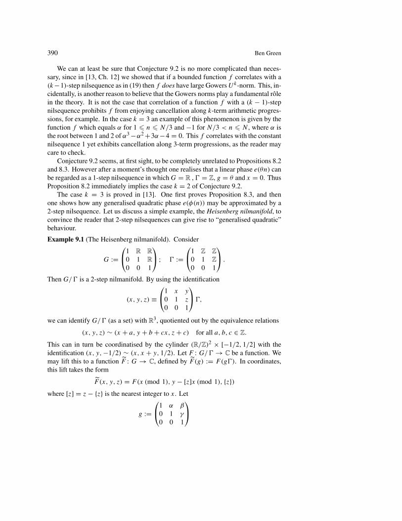
The case k = 3 is proved in [13]. One first proves Proposition 8.3, and thenone shows how any generalised quadratic phase e(φ(n)) may be approximated by a2-step nilsequence. Let us discuss a simple example, the Heisenberg nilmanifold, toconvince the reader that 2-step nilsequences can give rise to “generalised quadratic”behaviour.

Example 9.1 (The Heisenberg nilmanifold). Consider

G :=⎛⎝1 R R

0 1 R

0 0 1

⎞⎠ ; � :=⎛⎝1 Z Z

0 1 Z

0 0 1

⎞⎠ .

Then G/� is a 2-step nilmanifold. By using the identification

(x, y, z) ≡⎛⎝1 x y

0 1 z

0 0 1

⎞⎠ �,

we can identify G/� (as a set) with R3, quotiented out by the equivalence relations

(x, y, z) ∼ (x + a, y + b + cx, z + c) for all a, b, c ∈ Z.

This can in turn be coordinatised by the cylinder (R/Z)2 × [−1/2, 1/2] with theidentification (x, y, −1/2) ∼ (x, x + y, 1/2). Let F : G/� → C be a function. Wemay lift this to a function F : G → C, defined by F (g) := F(g�). In coordinates,this lift takes the form

F (x, y, z) = F(x (mod 1), y − [z]x (mod 1), {z})where [z] = z − {z} is the nearest integer to x. Let

g :=⎛⎝1 α β

0 1 γ

0 0 1

⎞⎠


be an element of G. Then the shift Tg : G → G is given by

Tg(x, y, z) = (x + α, y + β + γ x, z + γ ).

A short induction confirms, for example, that

T ng (0, 0, 0) = (nα, nβ + 1

2n(n + 1)αγ, nγ ).

Therefore if F : G/� → G/� is any Lipschitz function, written as a functionF : (R/Z)2 × [−1/2, 1/2] → C with F(−1/2, y, z) = F(1/2, y + z, z), then wehave

F(T ng (0, 0, 0)) = F(nα (mod 1), nβ + 1

2n(n + 1)αγ − [nγ ]nα (mod 1), {nγ }).The term [nγ ]nα which appears here certainly exhibits a sort of generalised

quadratic behaviour. For a complete description of how an arbitrary generalisedquadratic phase e(φ(n)) can be approximated by a two-step nilsequence, we refer thereader to [13, Ch. 12].

Let us conclude this section by stating, for the reader’s convenience, a result/con-jecture which summarises much of our discussion so far in one place.

Theorem 9.3 (Green–Tao [13]). We have the following two statements.

(i) (Generalised von Neumann) Suppose that s and t are positive integers withs + 2 � t . Suppose that A is a non-degenerate s × t matrix with integerentries. Suppose that f1, . . . , ft : [N ] → [−1, 1] are functions and that

|Ex1,...,xtAx=0

f1(x1) . . . ft (xt )| � δ. (20)

Then for each i = 1, . . . , t we have

‖fi‖Us+1 � cAδ.

(ii) (Gowers inverse result: proved for k = 2, 3, conjectural for k � 4) Supposethat f : [N] → [−1, 1] has ‖f ‖Uk � δ. Then there is a (k−1)-step nilmanifoldG/� with dimension at most C1,k(δ), together with a function F : G/� → C

with ‖F‖∞ � 1 and Lipschitz constant at most C2,k(δ) and elements g ∈ G,x ∈ G/� such that

|En�Nf (n)F (T ng · x)| � c3,k(δ). (21)

In particular when s = 1 or 2 and (20) holds for some A and some δ then for eachi = 1, . . . , t there is a 2-step nilsequence (F (T n

g · x))n∈N such that

|En�Nfi(n)F (T ng · x)| � cA(δ). (22)

392 Ben Green

10. Working with the primes

Let us suppose that we wish to count four-term progressions in the primes. One mighttry to apply Theorem 9.3 with the functions fi equal to the balanced function of A,the set of primes p � N , and then hope to rule out a correlation such as (21) for someδ = o(αt ) (here, of course, α ≈ log−1 N by the prime number theorem). This wouldthen lead to an asymptotic using various instances of (20) together with the triangleinequality.

There are two reasons why this is a hopeless strategy. First of all, the primes docorrelate with nilsequences. In fact since all primes other than 2 are odd it is easy tosee that

En�NfA(n)e(n/2) ≈ −α.

There is a way to circumvent this problem, which we call the W -trick. The idea isthat if W = 2 × 3 × · · · × w(N) is the product of the first several primes, then forany b coprime to W the set

Ab := {n � N : Wn + b is prime}does not exhibit significant bias in progressions with common difference q � w(N).One can then count 4-term progressions in the primes by counting 4-term progres-sions in Ab1 × . . . Ab4 for each quadruple (b1, . . . , b4) ∈ (Z/WZ)×4 in arithmeticprogression and adding.

We refer to any set Ab as a set of “W -tricked primes”. In practice one is onlyfree to take w(N) ∼ log log N , since one must be able to understand the distributionof primes in progressions with common difference W (note that even on GRH onecould only take w(N) ∼ c log N). Even assuming we could obtain optimal resultsconcerning the correlation of the W -tricked primes with 2-step nilsequences, thisinformation will be very weak indeed.

This highlights a more serious problem with the suggested strategy. Suppose thatA ⊆ [N] is a set of density α for which there is no obvious reason why A shouldhave an unexpectedly large or small number of 4-term APs, that is to say for whichwe might hope to prove that

Ex1,x2,x3,x4x1−2x2+x3=0x2−2x3+x4=0

1A(x1)1A(x2)1A(x3)1A(x4) ≈ α4. (23)

For example, A might be the W -tricked primes less than N , in which case α ∼W

φ(W)log−1 N .

We might prove (23) by writing 1A = α + fA, expanding as the sum of sixteenterms, and showing that fifteen of these are o(α4) by appealing to Theorem 9.3, andruling out a correlation with a 2-step nilsequence as in (22). Unfortunately we willbe operating with δ = o(α4) log−4+ε N , and the dependence of cA(δ) on δ is veryweak, being of the form exp(−δ−C). Thus we are asking to rule out the possibility


that|En�NfA(n)F (T n

g · x)| � exp(− logC N)

for some potentially rather large C. This is a problem, since one would never expectmore than square root cancellation in any such expression. In fact for the W -trickedprimes one only has a small amount (depending on w(N)) of potential cancellationto work with and to all intents and purposes one should not bank on having availableany estimate stronger than

En�NfA(n)F (T ng · x) = o(1).

What one really needs is a version of Proposition 16 which applies to functionswhich need not be bounded by 1. Then one could hope to work with the von Mangoldtfunction � instead of the far less natural characteristic function 1A, or more accuratelywith W -tricked variants of the von Mangoldt function such as

�b,W (n) := φ(W)

W�(Wn + b).

Such a result is the main result of our forthcoming paper [15]. It would take us toofar afield to say anything concerning its proof, other than that it uses one of the keytools from our paper [12] on long progressions of primes, the “ergodic transference”technology of [12, Chs. 6,7,8].

Proposition 10.1 (Transference principle, [15]). Suppose that ν : [N] → R+ is apseudorandom measure. Then

(i) The generalised von Neumann theorem, Theorem 9.3 (i), continues to hold forfunctions f1, . . . , ft : [N ] → R+ such that |fi(x)| � 1 + ν(x) pointwise (thevalue of cA may need to be reduced slightly).

(ii) If the Gowers inverse conjecture, Theorem 9.3 (ii), holds for a given value of k

then it continues to hold for a function f such that |f (x)| � 1+ν(x) pointwise.In particular such an extension of the Gowers inverse conjecture is true whenk = 2, 3.

The reader may consult [12, Ch. 3] for a definition of the term pseudorandommeasure and a discussion concerning it. For the purposes of this article the reader canmerely accept that there is such a notion, and furthermore that one may construct apseudorandom measure ν : [N] → R+ such that ν+1 dominates any fixed W -trickedvon Mangoldt function �W,b. The construction of ν comes from sieve theoretic ideasoriginating with Selberg. The confirmation that ν is pseudorandom is essentially due,in a very different context, to Goldston and Yıldırım [7].

Applying these two results, one may see that Conjecture 2.1 for a given non-degenerate s × t matrix A is a consequence of the Gowers inverse conjecture in thecase k = s + 1 together with a bound of the form

En�N(�b,W (n) − 1)F (T ng · x) = oG/�,F (1) (24)

394 Ben Green

for every s-step nilsequence (F (T ng · x))n∈N.

By effecting a decomposition of �b,W as �b,W + �

b,W rather like that in §4,

the proof of this statement may be further reduced to a similar result for the Möbiusfunction:

Conjecture 10.2 (Möbius and nilsequences). For all A > 0 we have the bound

En�Nμ(n)F (T ng · x) A,G/�,F log−A N

for every k-step nilsequence (F (T ng · x))n∈N.

Note that we require more cancellation (a power of a logarithm) here than in (24).This is because in passing from μ to �

b,W one loses a logarithm in performing

partial summation as in the derivation of (7). The method we have in mind to proveConjecture 10.2, however, is likely to give this strong cancellation at no extra cost.

Conjecture 10.2 posits a rather vast generalisation of Davenport’s bound. Theconjecture is, of course, highly plausible in view of the Möbius randomness law.

Let us remark that the derivation of (24) from Conjecture 10.2 is not at all imme-diate, since one must also handle the contribution from �

b,W . To do this one uses

methods of classical analytic number theory rather similar to those of Goldston andYıldırım [7].

11. Möbius and nilsequences

The main result of [14] is a proof of Conjecture 10.2 in the case k = 2. This leads,by the reasoning outlined in the previous section, to a proof of Conjecture 2.4 in thecase s = 2.

We remarked that the classical Hardy–Littlewood method was a technique ofharmonic analysis. We also highlighted the idea of dividing into major and minorarcs. We have said much on the subject of generalising the underlying harmonicanalysis, but as yet there has been nothing said about a suitable extension of majorand minor arcs. In this section we describe such an extension by making some remarksconcerning the proof of the case k = 2 of Conjecture 10.2.

In §5 we discussed how bounds on Type I and II sums may be used to show that agiven function f does not correlate with Möbius. Recalling our “inverse” strategy forproving Davenport’s bound, one might be tempted to go straight into Proposition 5.1with f (n) = F(T n

g · x), a 2-step nilsequence, posit largeness of either a Type I or aType II sum, and then use this to say that the nilsequence is somehow “major arc”.One might then hope to handle the major nilsequences by some other method, perhapsthe theory of L-functions.

Such an attempt is a little too simplistic, for the following reason. Returningto the 1-step case, note that the sum of two 1-step nilsequences is also a 1-stepnilsequence (on the product nilmanifold G1/�1 ×G2/�2). In particular, the function


f (n) = e(n/5) + e(n√

2) is a 1-step nilsequence. We know, however, that to handlecorrelation of Möbius with e(n/5) we need to know something about L-functions,whereas we do not have an L-function method of handling e(n

√2). This suggests

that some sort of preliminary decomposition of the function f is in order, and such asuggestion turns out to be correct.

In the 2-step case, a nilsequence F(T ng ·x) can be decomposed into local quadrat-

ics. These are objects of the form

f (n) := 1BN(n)e(φ(n)), (25)

where BN is a set of the form

BN := {n : N/2 � n < N : F1(n) �= 0}for some 1-step nilsequence F1 depending on F , G/�, g and x, and φ : BN → R/Z

is locally quadratic. This means that one may unambiguously define the secondderivative φ′′(h1, h2) to equal

φ(x + h1 + h2) − φ(x + h1) − φ(x + h2) + φ(x)

for any x such that x, x + h1, x + h2, x + h1 + h2 ∈ BN .It turns out that for the purposes of analysing Type I and II sums the cutoff 1BN

plays a subservient rôle. The phase φ, on the other hand, is crucial. The bulk of [14] isdevoted to showing that if either a Type I or a Type II sum involving some f as in (25)is large, then φ is major arc. This is a direct analogue of the proof of Davenport’sbound as phrased at the end of §5 (the “inverse” approach). Roughly speaking, φ

is said to be major arc if qφ′′(h1, h2) is small for some smallish q and all h1, h2,which in turn essentially means that φ is slowly varying on BN intersected with anyfixed progression a (mod q). For a detailed discussion see [14]. Suffice it to saythat the passage from large Type I/II sum to φ being major arc is long and difficult,and requires many applications of the Cauchy–Schwarz inequality to manipulate thephase φ into a helpful form, as well as basic tools of equidistribution such as a versionof the Erdos–Turán inequality.

Recalling Proposition 5.1, one has reduced the case s = 2 of Conjecture 10.2 tothe statement that

En�Nμ(n)1BN(n)e(φ(n)) A log−A N

for any major arc phase φ. It turns out that 1BN(n)e(φ(n)) can, in this case, be

closely approximated by a sum of linear phases e(θn), and so we may conclude usingProposition 4.1.

Note that this analysis has the flavour of an induction on s, the step of the nilse-quence we are considering. We expect to see this more clearly when addressing thegeneral case of Conjecture 10.2 in future work.

396 Ben Green

12. Future directions

The most obvious avenue of research left open is to generalise everything we havedone for s = 2 to the case s � 3. In particular we would like inverse theorems forthe Uk-norms for k � 4, and a proof of Conjecture 10.2 for s � 3. We are currentlyworking towards this goal. We expect that the methods of Gowers [10] can be adaptedto achieve the inverse theorem, though this will not be straightforward. It is also verylikely that the “inverse” approach to handling Type I and II sums can be adapted to thehigher-step case of Conjecture 10.2, though again we do not expect this to be whollystraightforward.

It would be very desirable to have good bounds for error terms such as the o(1) inTheorem 2.5. We are sure that our current estimate for the error in Theorem 2.5 is theworst that has ever featured in analytic number theory – the error term is a completelyineffective o(1)! Ultimately this is because to show that the error is less than δ onefinds oneself needing to rule out a real zero of some L(s, χ), χ a primitive quadraticcharacter to the modulus q, with s > 1 − Cq−ε, where ε = ε(δ) → 0 as δ → 0.Siegel’s theorem states that for any ε > 0 there is such a C, but it is, of course, notpossible to specify C effectively.

It is clear that the spectre of ineffectivity does not rear its head under the assumptionof GRH, and we believe that our methods lead to an error term of the form log−c N

in Theorem 2.5.There are other, presumably more tractible, ways in which one might obtain an

explicit error term. Improvements to the combinatorial tools used in [13], particu-larly advances on the circle of conjectures known as the “polynomial Freiman–Ruzsaconjecture”, could be very helpful here.

We turn now to goals which lie further away. I have hinted at various places inthis survey that the way in which we see nilsequences arising is very long-windedand, presumably, not the “right” way. The ergodic theorists [20], [35] do admittedlydiscover the rôle of these functions somewhat less painfully (albeit after setting up agood deal of notation). Nilsequences seem such natural objects, however, that thereought to be a much better way of appreciating their place in the study of systems oflinear equations. Recalling that ‖f ‖U2 is essentially the L4 norm of f one mighteven ask, for example,

Question 12.1. Is there a usable “formula” relating ‖f ‖U3 and certain of the “nil-fourier coefficients” En�Nf (n)F (T n

g · x)?

Such a formula would assuredly have to be very exotic on account of the vastprofusion of nilsequences which might enter into consideration. The nilsequencesare not naturally parametrised by anything so simple as the circle S1, which gave itsname to the classical circle method.

Let us conclude with some speculations on non-linear systems of equations, whereour knowledge is at present essentially non-existent. We have seen in Conjecture 9.2that the behaviour of an any system Ax = b, where A is non-degenerate in the sense


of Definition 2.3, should be governed by a very “hard” or “algebraic” collection ofcharacteristic functions, in this case the nilsequences.

On the other hand degenerate linear systems, such as x1 −x2 = 1, do not have thisproperty. To see this, suppose that N = 2m is even and let A ⊆ [N] be a set formedby setting A∩{2i, 2i +1} = {2i} or {2i +1}, these choices being independent in i fori = 0, . . . , m − 1. Then |A| = N/2, and A is indistinguishable from a truly randomset by taking inner products with any conceivable “hard” character such as a linear orquadratic phase. However, A is expected to have about N/8 solutions to x1 −x2 = 1,whereas a random set has about twice this many.

One might call an equation or system of equations for which a “hard” characteristicsystem exists a mixing system. We do not have a precise definition of this notion.Some non-linear equations are known to be mixing – for example, the linear phasese(θn) form a characteristic system for the equation x1 + x2 = x2

3 . Many moreare not. It would be very interesting to know, for example, whether the equationx1x2 − x3x4 = 1 is mixing and, if so, what a characteristic system for it might be.This seems to be a very difficult question as the analysis of this equation even in veryspecific situations involves deep methods from the theory of automorphic forms.

References

[1] Baker, R. C. and Harman, G., Exponential sums formed with the Möbius function. J.London Math. Soc. (2) 43 (2) (1991), 193–198.

[2] Balog, A., Linear equations in primes. Mathematika 39 (1992), 367–378.

[3] Bourgain, J., On triples in arithmetic progression. Geom. Funct. Anal. 9 (1999), 968–984.

[4] Chowla, S., There exists an infinity of 3-combinations of primes in A.P. Proc. Lahore.Philos. Soc. 6 (2) (1944), 15–16.

[5] Davenport, H., Multiplicative number theory. Third edition, Grad. Texts in Math. 74,Springer-Verlag, New York 2000.

[6] Furstenberg, H. and Weiss, B., A mean ergodic theorem for 1/N∑N

n=1 f (T nx)g(T n2x).

In Convergence in ergodic theory and probability (Columbus, OH, 1993), Ohio State Univ.Math. Res. Inst. Publ. 5, Walter de Gruyter, Berlin 1996, 193–227.

[7] Goldston, D. A. and Yıldırım, C. Y., Small gaps between primes, I. Preprint.

[8] Gowers, W. T., A new proof of Szemerédi’s theorem for arithmetic progressions of lengthfour. Geom. Funct. Anal. 8 (1998), 529–551.

[9] Gowers, W. T., Fourier analysis and Szemerédi’s theorem. In Proceedings of the Interna-tional Congress of Mathematicians (Berlin, 1998), Vol. I, Doc. Math., J. DMV, Extra Vol.ICM Berlin, 1998, 617–629.

[10] Gowers, W. T., A new proof of Szemerédi’s theorem. Geom. Funct. Anal. 11 (2001),465–588.

[11] Green, B. J., Long arithmetic progressions of primes. Preprint, submitted to Proceedingsof the Gauss-Dirichlet Conference, Göttingen 2005.

398 Ben Green

[12] Green, B. J. and Tao, T. C., The primes contain arbitrarily long arithmetic progressions.Ann. of Math., to appear.

[13] Green, B. J. and Tao, T. C., An inverse theorem for the Gowers U3-norm, with applications.Submitted.

[14] Green, B. J. and Tao, T. C., Quadratic uniformity of the Möbius function. Preprint.

[15] Green, B. J. and Tao, T. C., Linear equations in primes. In preparation.

[16] Hardy, G. H. and Littlewood, J. E., Some problems of “Partitio Numerorum”. III. On theexpression of a number as a sum of primes. Acta. Math. 44 (1923), 1–70.

[17] Hardy, G. H. and Littlewood, J. E., Some problems of “Partitio Numerorum”. V. A furthercontribution to the study of Goldbach’s problem. Proc. London Math. Soc. (2) 22 (1923),46–56.

[18] Hardy, G. H. and Ramanujan, S., Asymptotic formulæ in combinatory analysis. Proc.London Math. Soc. (2) 17 (1918), 75–115.

[19] Heath-Brown, D. R. Three primes and an almost prime in arithmetic progression. J. LondonMath. Soc. (2) 23 (1981), 396–414.

[20] Host, B. and Kra, B. Non-conventional ergodic averages and nilmanifolds. Ann. of Math.161 (1) (2005), 397–488.

[21] Iwaniec, H. and Kowalski, E. Analytic number theory. Amer. Math. Soc. Colloq. Publ. 53,Amer. Math. Soc., Providence, RI, 2004.

[22] Iwaniec, H., Luo, W and Sarnak, P., Low lying zeroes of families of L-functions. Inst.Hautes Études Sci. Publ. Math. 91 (2000), 55–131.

[23] Kra, B., The Green-Tao Theorem on arithmetic progressions in the primes: an ergodic pointof view. Bull. Amer. Math. Soc. 43 (2006), 3–23.

[24] Kra, B., From combinatorics to ergodic theory and back again. In Proceedings of theInternational Congress of Mathematicians (Madrid, 2006), Volume III, EMS PublishingHouse, Zürich 2006, 57–76.

[25] Kumchev, A. V. and Tolev, D. I., An invitation to additive prime number theory. SerdicaMath. J. 31 (1–2) (2005), 1–74.

[26] Salem, R. and Zygmund, A., Some properties of trigonometric series whose terms haverandom signs. Acta Math. 91 (1954), 245–301.

[27] Tao, T. C.,Arithmetic progressions and the primes. El Escorial Proceedings 2004, to appear.

[28] Tao, T. C., Obstructions to uniformity, and arithmetic patterns in the primes. Preprint.

[29] Van der Corput, J. G., Über Summen von Primzahlen und Primzahlquadraten. Math. Ann.116 (1939), 1–50.

[30] Vaughan, R. C., Sommes trigonométriques sur les nombres premiers, C. R. Acad. Sci. ParisSér. A 285 (16) (1977), A981–A983.

[31] Vaughan, R. C., Hardy’s Legacy to Number Theory. J. Austral. Math. Soc. Ser. A 65 (1998),238–266.

[32] Vaughan, R. C. and Wooley, T. D., Waring’s problem: a survey. In Number theory for themillennium, III (Urbana, IL, 2000), A K Peters, Natick, MA, 2002, 301–340.

[33] Vinogradov, I. M., Representation of an odd number as the sum of three primes. Dokl.Akad. Nauk SSSR 15 (1937), 291–294.


[34] Wooley, T. D., Diophantine problems in many variables: the rôle of additive number theory.In Topics in Number Theory (ed. by S. D. Ahlgren et al.), Kluwer Academic Publishers,Dordrecht 1999, 49–83.

[35] Ziegler, T., Universal characteristic factors and Furstenberg averages. J. Amer. Math. Soc.,to appear.

School of Mathematics, University Walk, Bristol BS8 1TW, EnglandE-mail: [email protected]

Documents

Generalising the Hardy–Littlewood method for primesicm2006.org › proceedings › Vol_II › contents › ICM_Vol_2_17.pdf · The Hardy–Littlewood method is a well-known technique