Embed Size (px)
Citation preview

General Growth Mixture Analysis 1
General Growth Mixture Analysis
with Antecedents and Consequences of Change*
by
Hanno Petras & Katherine Masyn**
In:
Piquero, A. & Weisburd, D.: Handbook of Quantitative Criminology
*We like to thank Alex Piquero, David Weisburd, Nicholas Ialongo and Bengt Muthén for their
helpful comments on a prior draft of this manuscript.
**The order of the authors was determined by randomization

General Growth Mixture Analysis 2
Introduction
Describing and predicting the developmental course of individuals’ involvement in
criminal and antisocial behavior is a central theme in criminological inquiries. A large body of
evidence is available documenting that individual differences in levels of criminal behavior
across time can effectively be described qualitatively using a discrete number of criminal career
patterns which vary by age of onset, career length, as well as type and frequency of the behavior.
The majority of studies, using selective offender or population-based samples, have identified
offending typologies made up of four to six distinct trajectory profiles. Most of these profiles are
declining and are distinguished by the level of offending at their peak and the timing of the
decline (Piquero, 2008). For example, Sampson & Laub (2003) identified several distinct
offending trajectories patterns. One small group of individuals (3%) peaked in their offending
behavior in the late 30s and declined to almost “0” at age 60 and were labeled "high-rate
chronics". In addition, three desisting groups were identified, who declined after middle
adolescence, late adolescence and early adulthood, respectively. Finally, a small group (8%)
followed a low-rate chronic offending patterns between the ages of 19 and 39, and declined
thereafter.
Childhood aggressive behavior is widely recognized as a precursor for antisocial and
criminal behavior in adolescence and adulthood. Numerous prospective studies have
demonstrated that conduct problems (as early as preschool) predict later delinquent behavior and
drug use (Ensminger et al., 1983; Hawkins et al., 2000; Lynam, 1996; McCord and Ensminger,
1997; Yoshikawa, 1994). Motivated by developmental research (Loeber and Hay, 1997; Moffit,
1993; Patterson, DeBaryshe, & Ramsey, 1989), a large body of longitudinal research has

General Growth Mixture Analysis 3
identified several developmental prototypes for individuals that vary in onset and course of
aggressive behavior (Broidy et al, 2003; Dulmen, Goncy, Vest, & Flannery, 2008; Nagin &
Tremblay, 1999; Schaeffer et al., 2006; Petras et al., 2004; Petras et al., 2008; Shaw, Gilliom,
Ingoldsby, & Nagin, 2003 ). Despite differences in terminology and emphasis, each study
identifies two to five distinct patterns of youth antisocial behavior over time with different
behavior trajectories, risk factors, and prognoses for desistence from antisocial behavior as
adults. Each proposed typology includes one to two chronic profiles with early and persistent
aggression that is likely to be related to a biological or genetic vulnerability, exacerbated by poor
parenting and early school failure. Each also identifies one or two less severe profiles with
antisocial behavior that starts later, is less aggressive, is more sporadic, and stems from later
socialization experiences such as deviant peer affiliations in early adolescence. Implicit in each
typology is also the assumption that there is at least one other profile that characterizes youth
who do not exhibit problems with antisocial behaviors. Additional evidence suggests that there is
also a profile characterizing the substantial proportion of those children who display high levels
of aggressive behavior in childhood but who do not manifest antisocial behavior in adolescence
or adulthood (Maughan & Rutter, 1998).
In summary, many of the studies of youth, adolescents, and adults related to delinquent,
antisocial, and criminal offending, have utilized a language of trajectory typologies to describe
the individual differences in the behavioral course manifest in their longitudinal data. Although
this language maps well onto some of the corresponding theories that provide the conceptual
frameworks for these empirical investigations, the majority of these studies have not relied on
subjective or heuristic taxonomies but instead relied on empirically-derived taxonomies based on
statistical modeling techniques, analogous to clustering and, by doing so, have been able to

General Growth Mixture Analysis 4
progressively evaluate the veracity of the underlying theories themselves. The two most
common statistical methods currently in use are the semi-parametric group-based modeling, also
known as latent class growth analysis (LCGA; Nagin & Land, 1993; Roeder, Lynch, & Nagin,
1999; Nagin, 2005), and general growth mixture analysis (GGMA; Muthén, 2001, 2002, 2004;
Muthen & Asparouhov, 2008; Muthén & Muthén, 1998-2008; Muthén & Shedden, 1999).
Although there are differences in model specification and estimation (see the chapter in this
handbook for more information on LCGA), both methods characterize some portion of the
systematic population heterogeneity in the longitudinal process under study (i.e., between-
individual variability not due to time-specific or measurement error) in terms of a finite number
of trajectories groups (latent growth classes or mixture components) for which the mean or
average growth within each group typifies one of the growth patterns or profiles manifest in the
population. Together, the studies employing these methods have helped to shift the study of
antisocial and criminal behavior away from what has been termed a “variable-centered” focus,
describing broad predictors of behavior variance, toward a more “person-centered” focus,
emphasizing discretely distinct individual differences in development (Magnusson, 1998).
In concert with the growing popularity of these data-driven, group-based methods for
studying developmental and life-course behavior trajectories has come active and spirited
ontological discussions about the nature of the emergent trajectory groups resulting from the
analyses (Bauer & Curran, 2003, 2004; Nagin & Tremblay, 2005; Sampson, Laub, & Eggleston,
2004; Sampson & Laub, 2005), i.e., whether the resultant trajectory typology defined by the sub-
groups derived from the data represent a “true” developmental taxonomy. Further debate
involves whether it is reasonable to even apply these methods if there is not a true taxonomy
underlying the data, under what conditions these methods should be applied, and how the results

General Growth Mixture Analysis 5
should be interpreted if we consider the fact that, for any given data set, we cannot know the
“truth” of the population distribution from which the observations were drawn. For example, we
may not be able to make an empirical distinction between a sample of observations drawn from a
population of values with a bimodal distribution and a sample of observations drawn from a
mixture of two normally distributed subpopulations. Likewise, we may have a sample of
observations for which a model that assumes a bimodal distribution is statistically
indistinguishable from a model that assumes a finite mixture of two normal components. Thus,
as is the case with any statistical modeling, the data can only empirically distinguish between
models more or less consistent with the observations in the sample−they cannot identify the
"truth" of the population between models with equivalent or nearly equivalent goodness-of-fit.
Unfortunately, this issue of the True population distribution, i.e., the verity of the existence of
latent subgroups in a given population, cannot be solved by means of replication since a new
sample will give a similar distribution with similar ambiguities about the characteristics of the
population distribution.
For the purposes of this chapter, we acknowledge that these debates are ongoing, but
believe that the usefulness of these group-based models does not hinge on the ontological nature
of the resultant trajectory groups. We presuppose that there are analytic, empirical, and
substantive advantages inherent in using discrete components to (partially) describe population
heterogeneity in longitudinal processes regardless of whether those discrete components are an
approximation of a continuum of variability or if the components represent actual unobserved
sub-populations within the larger population under study. In this chapter, we focus instead on
the use of auxiliary information in terms of antecedents (predictors and covariates) and
consequences (sequelae and distal static outcomes) of trajectory group membership in the

General Growth Mixture Analysis 6
GGMA framework (Muthén, 2006). The use of auxiliary information, potentially derived from
substantive theory, is highly relevant to determine the concurrent and prognostic validity of
specific developmental trajectory profiles derived from a particular data set (Bushway, Brame,
Paternoster, 1999; Heckman & Singer, 1984, Kreuter & Muthén, 2008). That is to say, the
inclusion of auxiliary information in a growth mixture analysis is a necessary step in
understanding as well as evaluating the fidelity and utility of the resultant trajectory profiles from
a given study, regardless of one’s beliefs about the veracity of the method itself. The remainder
of the chapter is organized as follows: First, we briefly introduce the conventional latent growth
curve model followed by a presentation of the unconditional growth mixture model, of which the
latent growth curve model and latent class growth model are special cases. We then discuss the
process for including antecedents and consequences of change in the general growth mixture
analysis (GGMA) framework. We conclude this chapter with an empirical example using data
from a large randomized trial in Baltimore.
The Unconditional Latent Growth Curve Model
Repeated measures on a sample of individuals results in a particular form of multilevel
data, where time or measurement occasions at “Level 1” are nested within persons at “Level 2”.
This data can be analyzed using a multilevel modeling framework where intraindividual change
is described as a function of time and interindividual differences are described by random effects
and coefficients (Multilevel Linear Models - MLM or Hierarchical Linear Models - HLM;
Raudenbush & Bryk, 2002; Hox, 2000, 2002). Alternatively, a multivariate latent variable
approach can be used where the parameters of the individual growth curves are modeled as latent
variables (e.g., latent intercept and slope factors), with a covariance and mean structure (Latent
Growth Curve Models - LGCM, Latent Growth Models - LGM, or Latent Variable Growth

General Growth Mixture Analysis 7
Models - LVGM; Meredith & Tisak, 1990; Willet & Sayer, 1994; Muthén, 2004). A typical
unconditional linear latent growth curve model with T time points and n individuals is specified
below.
0
0 00 0
0 1
Level 1:
,
Level 2:
,
,
ti i si ti ti
i i
si s i
y a
(1)
where
~ ( , ),
~ ( , ),
( , ) 0.
MVN
MVN
Cov
ε 0 Θ
ζ 0 Ψ
Here, tiy is the observed outcome y for individual i (i = 1,...,n) at time t (t = 1,...,T), tia is the time
score for individual i at time t, 0i is the random intercept factor (i.e., the "true score" value for
individual i at time ati=0), and si is the random linear slope factor (i.e., the expected change in
yi for a one unit increase in time, on the scale of at). In latent variable modeling terms, the ty 's
are the indicators or manifest variables for the latent growth factors, 0 and s . ti represent
measurement and time-specific error at time t and the t 's are usually assumed to be

General Growth Mixture Analysis 8
uncorrelated; however, that restriction can be relaxed. In the more traditional matrix notation of
the latent variable framework, the equations in (1) can be written as
,
,
i i i
i i
Y Λη ε
η α ζ
(2)
where iY is a (Tx1) vector of observed scores for individual i, iη is a (px1) vector of growth
factors, Λ is a (Txp) design matrix of factor loadings with each column corresponding to specific
aspects of change, and α is a (px1) vector of growth factor means. In this specification,
,ti ta a i , but it is possible to incorporate individual-varying times of measurement within this
framework by treating time measures at each occasion as a time-varying covariate with a random
effect. For a linear model, p=2, the loading matrix is given by
1
2
1
1
1
s
s
sT
(3)
where the loading values in the second column would be fixed to define the slope factor as the
linear rate of change on the observed time metric; for example, (0,1,2,..., 1) 's T λ . Typically,
the first loading, 1s , is fixed at zero so that the intercept factor can be interpreted as the
response at the first time of measurement (t=1). Although the above specification expresses the
change in the outcome as a linear function of the time metric, it is possible (with an adequate
number of repeated observations on each subject) to investigate interindividual differences in
nonlinear trajectories of change. The most common approach is the use of polynomials where
additional factors (p>2) represent quadratic or cubic functions of the observed time metric.

General Growth Mixture Analysis 9
Nested models with increasing numbers of growth factors are assessed by chi-square difference
testing as well as the use of SEM fit indices (Hu & Bentler, 1999). Alternative specifications of
time can also be easily accommodated, including piece-wise linear growth models as well as
exponential and sinusoidal models of change. Also, it is possible for the Level 1 equation in (1)
and the residual variance/covariance structure of Y to be specified as a generalized linear model
to accommodate binary, multinomial, ordinal, and count measures for the change process in
addition to continuous measures. The path diagram for the unconditional linear latent growth
curve model is shown in Figure 1.
Although it is possible to specify analytically-equivalent unconditional models across the
multilevel and latent variable modeling frameworks, utilizing the latent variable approach affords
access to a variety of modeling extensions not as easily implemented in other frameworks, e.g.,
models that simultaneously include both antecedents and consequences of the changes process;
higher order growth models with multiple indicators of the outcome at each assessment; multi-
process and multilevel growth models; and models that employ both continuous and categorical
latent variables for describing population heterogeneity in the change process (for more on
growth modeling in a latent variable framework, see, for example, Bollen & Curran, 2006;
Duncan, Duncan, & Strycker, 2006; Muthén, 2001, 2004). In the next section, we describe the
last extension for which the latent growth curve model serves as a foundational and restricted
case in the broader category of general growth mixture models.
The Unconditional General Growth Mixture Model
General growth mixture analysis (GGMA) stands at the intersection of latent growth
curve modeling and finite mixture modeling. In finite mixture modeling, rather than making the

General Growth Mixture Analysis 10
usual assumption that the observed responses in a data sample are identically distributed, i.e., are
drawn from a singular homogeneous population, it is assumed that the data are drawn from a
finite number of heterogeneous subpopulations. The finite mixture analysis divides the
population into an unknown number of exhaustive and mutually exclusive subpopulations (or
latent classes), each with its own response distribution. Figure 2 illustrates a mixture of two
normally-distributed subpopulations. In the latent variable framework, the mixtures, or
subpopulations, are represented by categories of a latent multinomial variable, usually termed a
latent class variable. And the mixture components or subpopulations are referred to as latent
classes. The distribution of an observed outcome, iY is a mixture distribution defined as
1
( ) Pr( ) ( | ) ,K
i i i i
k
f C k f C k
Y Y (4)
where iC represents the latent class membership for individual i, K is the total number of latent
classes (subpopulations), Pr( )iC k is the mixing proportion for Class k, and ( | )i if C kY is
the class-specific response distribution of iY .
Latent class membership is unobserved and is determined by the class-specific model
parameters. This brings us to a critical point, which we will emphasize repeatedly in this
chapter. As with any latent variable, it is necessary to specify a measurement model for the
latent class variable. Indicators for the latent class variable include any variables, observed or
latent, that differ in values between individuals in the population due to latent class membership,
as well as model parameters that are permitted to be class-specific, thereby designating those
parameters as individually-varying or “random” effects in the given model. The latent classes
are then characterized by the class-specific joint distribution of all those variables and random

General Growth Mixture Analysis 11
effects and empirically based on the overall joint distribution in the sample. Thus, the estimation
of the optimal number and size of the latent classes (class proportions), as well as the
corresponding model parameter estimates (class-specific and overall) and interpretation of the
resultant classes, will very much depend on: 1) which variables and random effects are included
as latent class indicators and 2) the specification of the within-class joint distribution of those
latent class indicators. This is analogous to selecting the attribute space and the resemblance
coefficient in a cluster analysis. For example, if we specified a latent class model in which the
classes differed only with respect to their mean structure and assumed conditional independence
of all the class indicators, we may extract different classes (number, size, and class-specific
parameters estimates) than a model in which the classes differed with respect to both their mean
and variance-covariance structure.
In growth mixture modeling, rather than assuming the individual growth parameters (e.g.,
individual intercept and growth factors) are identically distributed, i.e., are drawn from a singular
homogeneous population, as we do in latent growth curve modeling, it is assumed that the
individual growth parameters are drawn from a finite number of heterogeneous subpopulations.
The growth mixture analysis divides the population into an unknown number of exhaustive and
mutually exclusive latent trajectory classes, each with a unique distribution of individual growth
factors. In other words, the continuous latent growth factors serve as the indicators for the K-
category latent class variable, C, in a growth mixture model, as expressed below.
,
,
i i i
i k i
Y Λη ε
η α ζ
(5)
where
General Growth Mixture Analysis 12
0
0
1
~ ( , ),
~ ( , ),
exp( )Pr( ) .
exp( )
k
k
ki K
h
h
MVN
MVN
C k
ε 0 Θ
ζ 0 Ψ
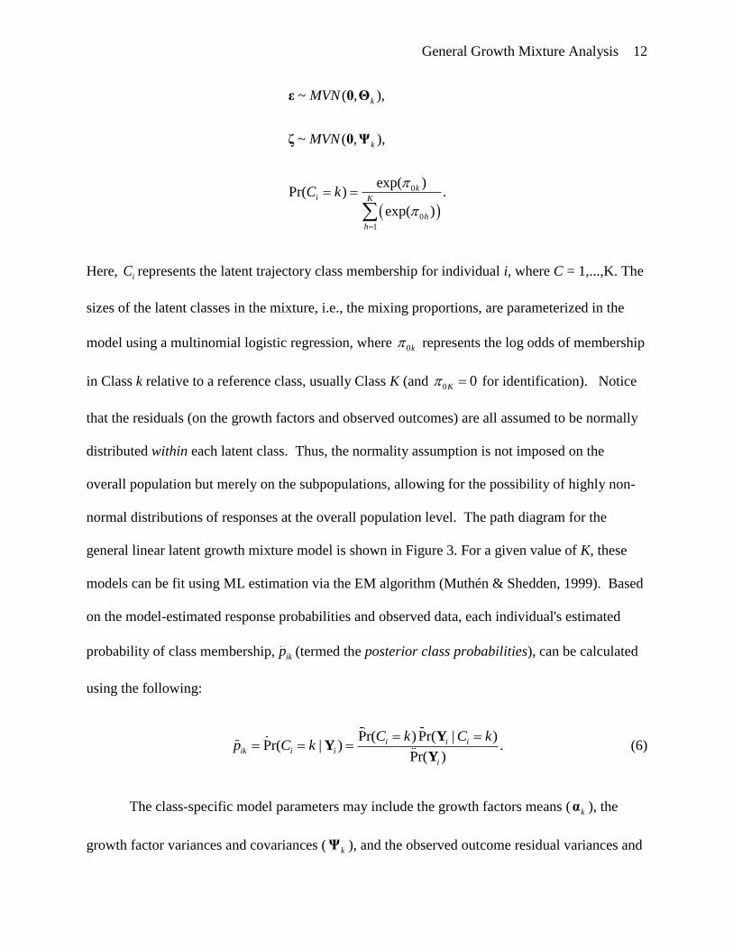
Here, iC represents the latent trajectory class membership for individual i, where C = 1,...,K. The
sizes of the latent classes in the mixture, i.e., the mixing proportions, are parameterized in the
model using a multinomial logistic regression, where 0k represents the log odds of membership
in Class k relative to a reference class, usually Class K (and 0 0K for identification). Notice
that the residuals (on the growth factors and observed outcomes) are all assumed to be normally
distributed within each latent class. Thus, the normality assumption is not imposed on the
overall population but merely on the subpopulations, allowing for the possibility of highly non-
normal distributions of responses at the overall population level. The path diagram for the
general linear latent growth mixture model is shown in Figure 3. For a given value of K, these
models can be fit using ML estimation via the EM algorithm (Muthén & Shedden, 1999). Based
on the model-estimated response probabilities and observed data, each individual's estimated
probability of class membership, ikp (termed the posterior class probabilities), can be calculated
using the following:
Pr( )Pr( | )
Pr( | ) .Pr( )
i i iik i i
i
C k C kp C k
YY
Y (6)
The class-specific model parameters may include the growth factors means ( kα ), the
growth factor variances and covariances ( kΨ ), and the observed outcome residual variances and

General Growth Mixture Analysis 13
covariances ( kΘ ). However, as we mentioned before, one must give careful consideration to
what is permitted to vary across the classes for it is those differences that define the classes
themselves. Thus, if we wanted latent classes or mixtures that partitioned the population on the
basis of differences in the systematic change process over time, i.e., mixture based exclusively
on the joint distribution of latent growth factors, then we may not want to allow the outcome
residual variances and covariances to be class-specific, i.e., we may want to constrain
,k k Θ Θ . As another example, if we changed the location of the intercept growth factor by
centering the time scale at the end of the time range instead of the beginning, then the latent
classes would be characterized by heterogeneity in the outcome level at the final time point and
the outcome change over time rather than by heterogeneity in the outcome level at the first time
point and outcome change over time. Only in models with kΨ unstructured and unconstrained
across the latent classes will the maximum likelihood value be the same regardless of the time
centering.
It is clear to see from the equations in (5) that the latent growth curve model describe in
the previous section is simply a growth mixture model with K=1. Another special case is the
latent class growth model developed by Nagin and colleagues (Nagin, 1999; Nagin & Land,
1993; Nagin, 2005; Roeder, Lynch, & Nagin, 1999; Jones, Nagin & Roeder, 2001) which is
characterized by zero within-class growth factor variance and covariances, thus assuming
homogeneity of individuals’ systematic development within a particular class, i.e., ,k k Ψ 0 .
Not only does this stand as a special case of growth mixture modeling, it represents a very
specific measurement model for the latent class variable portion such that the classes are
differentiated by differences in the mean structure on the growth factors with all interindividual

General Growth Mixture Analysis 14
variability on the growth factors and covariance between the growth factors explained by latent
class membership. Certainly, the necessary number and nature of the latent classes extracted
from a given data set under this model specification will deviate from those extracted using a
different measurement model specification. To be more specific, a greater number of latent
classes would be needed for a model in which all growth factor variance and covariance had to
be captured by between-class differences compared to a model in which overall growth factor
variance and covariance were partitioned into inter-class and intra-class variability. Models that
assign all systematic variability in growth to class membership are usually less parsimonious but
are more flexible and make fewer parametric assumptions. Interestingly, although the latent
class growth model may be more parameter-laden, it may be easier to estimate, i.e., converge
more readily, than a less constrained model with fewer classes but an equivalent number of free
parameters, especially in cases for which the overall variability in one or more of the growth
factors is small. In those cases, even with fewer classes, there may not be enough overall
variance to parse out across the between- and within-class differences, leading to an empirical
identification problem. Unfortunately, these are not problems that can be readily foreseen ahead
of the actual data analysis and must be dealt with as it arises. Models with different within- and
between-class differences can be compared in terms of relative goodness-of-fit using various
information indices; however, nested models that differ in the number of latent classes cannot be
compared using a standard chi-squared approximation for the likelihood ratio test (LRT), as is
explained in the following section on model building (although alternatives are suggested).
Additionally, a K-class model with ,k k Ψ 0 , cannot be directly compared to a K-class model
with unconstrained kΨ using a standard chi-squared approximation for the LRT because the null

General Growth Mixture Analysis 15
hypothesis lies on the boundary of the parameter space defined by the alternative (Stram & Lee,
1994).
Model Building in GGMA
Given the complexity of the model and the different measurement model specifications
for the latent class variable, it is recommended that model building proceed in a systematic step-
wise fashion. The first step in the process is specifying the functional form for individual change
over time. Descriptive analyses at this first foray into the data can reveal commonalities across
individuals and idiosyncrasies between individuals with respect to each person’s pattern of
growth over time. It is important to note that the shape of the mean change trajectory in the
overall sample may not mirror the shape of individual trajectories within that sample. Thus, it is
critical to examine smooth nonparametric as well as OLS trajectories across at least a random
sample of subjects in the dataset to explore the shapes of individual change over time. In
selecting a functional form, e.g. linear or curvilinear, one should consider adopting the most
parsimonious choice that will adequately describe the individual trajectories, allowing for the
fact that plots based on repeated measures of single subjects will reflect both systematic changes
over time as well as random fluctuation due to measurement and time-specific error. (For more
on this descriptive step, see, for example, Singer & Willett, 2003.)
The next step in the model building process is class enumeration. All of the mixture
model specifications in the previous section were predicated on a known value for K. Although
we may have very compelling substantive theories, as discussed in the introduction, regarding
discrete typologies of change or growth, these theories are rarely specific enough to guide a
purely confirmatory model fitting process, e.g., "we hypothesize three latent trajectory classes

General Growth Mixture Analysis 16
with class-specific quadratic mean structures, class-specific growth factor variances, zero within-
class growth factor covariances, and class-invariant outcome residual variances." Thus, the class
enumeration process advances in more exploratory manner while giving due consideration to a
prior substantive hypotheses regarding the number and nature of the subpopulations that may be
represented in the data. (Recall that the use of mixtures may be as much for accommodating
non-normality in the overall population as uncovering "true" subpopulations.)
This step begins by considering a set of models with an increasing number of latent
classes under a given measurement model. It is advisable to begin with a somewhat restricted
measurement model given some of the known pitfalls in mixture model estimation. Mixture
models can have difficulty with convergence and a model specification that allows the growth
factor (or outcome) residual variances to differ across class results in an unbounded likelihood
function which can increase the chance of non-convergence because the candidate parameter
space may include solutions with variances of zero and latent classes made up of single
individuals (McLachlan & Peel, 2000). This, coupled with the previous discussed motivation,
suggests beginning the class enumeration process with a measurement model for
which ,k k Θ Θ . We may similarly consider constraining ,k k Ψ Ψ in our initial model
specification as well. However, rather than assuming that the covariances between the growth
factors within each latent class are the same, it may be more reasonable to start with a model
that, like traditional latent class and latent profile analysis, assumes conditional independence of
the class indicators, i.e., fixes the covariances of the growth factors within class to zero such that
the growth factors are independent conditional on latent class. In such a model, the latent class
variable would be designed to account for (or explain) all of the covariance between the growth
factors in the overall population while the overall variance of the growth factors would be

General Growth Mixture Analysis 17
accounted for in part by the within-class continuous random variability on the growth factors and
in part by the between-class differences in growth factor means. Thus, beginning ultimately with
a measurement model where 1( ,..., )k pDiag Ψ and ,k k Θ Θ , with kα free to vary across
the K latent classes. This particular specification represents a probabilistic variant of a k-means
clustering algorithm applied to the “true” growth factor values for the individuals in the sample
(Vermunt & Magidson, 2002). Once the class enumeration step is complete, one could
theoretically use nested model tests and fit indices to investigate whether freeing the growth
factor variances across the latent classes or relaxing the conditional independence assumption
improves the fit of the model. However, by making such changes to the latent class
measurement model specification, we should not be surprised if we see not only changes to the
relative fit of the model, but also significant changes to the location, size, and substantive
meaning of the latent classes. If this occurs, we may be given cause to reevaluate the final
model selection from the latent class enumeration step or, more drastically, to reconsider the
model specification used for the latent class enumeration process itself, and begin again.
Mixture models are also infamous for converging on local rather than global maxima
when they do converge. The use of multiple starts from random locations in the parameter space
can improve chance of convergence to global maxima (Hipp & Bauer, 2006). Ideally,
replication of the maximum likelihood value across a large number of random sets of start values
increases confidence that the solution obtained is a global maximum.
Once a set of models, differing only in the number of classes, has been estimated, the
models are then compared to make a determination as to the smallest number of classes
necessary to effectively describe the heterogeneity manifest through those classes. This first step
in growth mixture modeling −deciding on the appropriate number of classes− can prove the most

General Growth Mixture Analysis 18
taxing, particularly because there is no single method for comparing models with differing
numbers of latent classes that is widely accepted as best (Muthén & Asparouhouv, 2008; Nylund,
Asparouhov, & Muthén, 2007); but by careful and systematic consideration of a set of plausible
models, and utilizing a combination of statistical and substantive model checking (Muthén,
2003), researchers can improve their confidence in the tenability of their resultant model
selection. Comparisons of model fit are based primarily on the log likelihood value. The
standard chi-square difference test (likelihood ratio test; LRT) cannot be used in this setting,
because regularity conditions of the test are violated when comparing a k-class model to a (k-g)-
class model (McLachlan & Peel, 2000). However, two alternatives, currently implemented in
the Mplus V5.1 software (Muthén & Muthén, 1998-2008), are available: 1) The Vuong-Lo-
Mendell-Rubin test (VLMR-LRT; Lo, Mendell, & Rubin, 2001) analytically approximates the
LRT distribution when comparing a k-class to a (k-g)-class finite mixture model for which the
classes differ only in the mean structure, and 2) The parametric bootstrapped LRT (BLRT),
recommended by McLachlan and Peel (2000), uses bootstrap samples (generated using
parameter estimated from a (k-g)-class model) to empirically derive the sampling distribution of
the LRT statistic. Both of these tests and their performance across a range of finite mixture
models is explored in detail in the simulation study by Nylund et al. (2007). As executed in
Mplus, these tests compare a (k-1)-class model (the null model) with a k-class model (the
alternative, less restrictive model) and a statistically significant p-value suggests the k-class
model fits the data better than a model with one fewer classes. In addition to these tests,
likelihood-based information indices, such as the Bayesian Information Criterion (BIC; Schwarz,
1978) are used in model selection. This index and similar ones (e.g., sample-size adjusted BIC)
are computed as a function of the log likelihood with a penalty for model complexity (e.g., the

General Growth Mixture Analysis 19
number of parameters estimated relative to the sample size). In general, a lower value on an
information criterion indicates a better model. Based on their simulation work, Nylund et al.
(2007) recommend using the BIC and VLMR-LRT to trim the set of models under consideration
and then including the BLRT for a smaller set of model comparisons (due to the computational
demands of the BLRT).
Although the model likelihood will always improve with an increasing number of classes,
sometimes none of the other fit indices reach a clear optimal value among the set of candidate
model. For example, the BIC may never arrive at a single lowest value at some value for K and
then begin to increase for all models with more than K classes, or the VLMR-LRT and BLRT
may never return a significant p-value, favoring a (k-1)-class model over a k-class model, before
the number of classes is increased to the point at which the model no longer converges to a
proper solution or fails to converge at all. However, in these cases, we can loosely explore the
diminishing gains in model fit according to these indices with the use of “elbow” plots. For
example, if we graph the maximum log likelihood values models with an increasing number of
classes, the addition of the second and third class may add much more information, but as the
number of classes increases, the marginal gain may drop, resulting in a (hopefully) pronounced
angle in the plot. The number of classes at this point meets the “elbow criterion” for that index.
We could make a similar plot for BIC values. Analogous to the scree plot for principal
component analysis, we could also plot the percent of total growth factor variance explained by
the latent classes for each class enumeration, i.e., the ratio of the between-class growth factor
variance for the total variance (Thorndike, 1953). In addition to these elbow plots, graphic
representations of each of the multivariate observations themselves could be used to guide in
reducing the set of candidate models such as the tree plots suggested by Lubke and Spies (2008).

General Growth Mixture Analysis 20
It can be noted that the set of the model comparisons discussed above are relative model
comparisons, and evaluations of overall goodness-of-fit are conspicuously absent. For example,
all of the relative comparisons may favor, say, a 3-class model over a 2-class model as a better fit
to the data, but none of the fit indices or tests indicate whether either is a good fit to the data.
However, depending on the measurement scale of the outcome variable and the presence of
missing data, there are some model diagnostics available for overall goodness-of-fit. If the
observed outcome variables are binary, ordinal, or count, it is possible to compute the overall
univariate, bivariate, and multivariate model-estimated response pattern frequencies and relative
frequencies for Y , along with the corresponding standardized Pearson residuals. For continuous
outcome variables, it is possible to compute the overall model-estimated means, variances,
covariances, univariate skewness, and univariate kurtosis, along with the corresponding
residuals. In each case, the overall model-estimated values are computed as a mixture across the
latent classes. Additional residual graphical diagnostics designed to detect misspecification in
growth mixture models regarding the number of latent trajectory classes, the functional form of
the within-class growth trajectory (i.e., functional relationship between the observed outcome
and time), and the within-class covariance structure are presented in a paper by Wang, Brown,
and Bandeen-Roche (2005) but are not currently implemented directly in the software most
commonly used by researchers in applied settings for growth mixture modeling.
In addition to the statistical criteria discussed above, it is also useful assess the value and
utility of the resultant classes themselves. One measure which can be used for this purpose is
entropy (Ramaswamy, Desarbo, Reibstein, & Robinson, 1993). Entropy summarizes the degree
to which the latent classes are distinguishable and the precision with which individuals can be
placed into classes. It is a function of the individual estimated posterior probabilities and ranges

General Growth Mixture Analysis 21
from 0 to 1 with higher values indicating better class separation. Entropy is not a measure of fit,
nor was it originally intended for model selection; however, if the intended purpose of the
growth mixture model is to find homogeneous groupings of individuals with characteristically
distinct growth trajectories, such that the between-class dispersion is much greater than the
within-class dispersion, then low values of entropy may indicate that the model is not well
serving its purpose (e.g., Nagin, 1999).
Beyond all these measures, it is also important to make some qualitative evaluations of
the usefulness and face validity of the latent class extractions by examining and interpreting the
estimates and corresponding plots of the model-implied mean class trajectories for different
models. If the model permits class-specific growth factor variances and covariances, it would be
informative to also examine scatterplots of the estimated individual growth factor scores
according to either modal latent class assignment or by pseudo-class draw (explained in a later
section) since classes would be distinguished by both the mean and variance-covariance
structure. It may also be worthwhile noting class size and proportions since an over-extraction of
classes might be revealed through particularly small and non-distinct classes emerging at higher
enumerative values. Further validation of the primary candidate models can also be done. If
there is an ample enough sample size, it is possible to carry out a split sample validation by
conducting the exploration of latent structure on one random half of the sample and then
evaluating the fit of the selected model on the second half of the sample. Additionally, auxiliary
information, potentially derived from substantive theory, in the form of antecedent and
consequent variables of the latent construct can be examined to evaluate the concurrent and
prognostic validity of the latent structure as specified in a given model (Muthén, 2003). How
this auxiliary information may be included is the topic of the next section.
General Growth Mixture Analysis 22
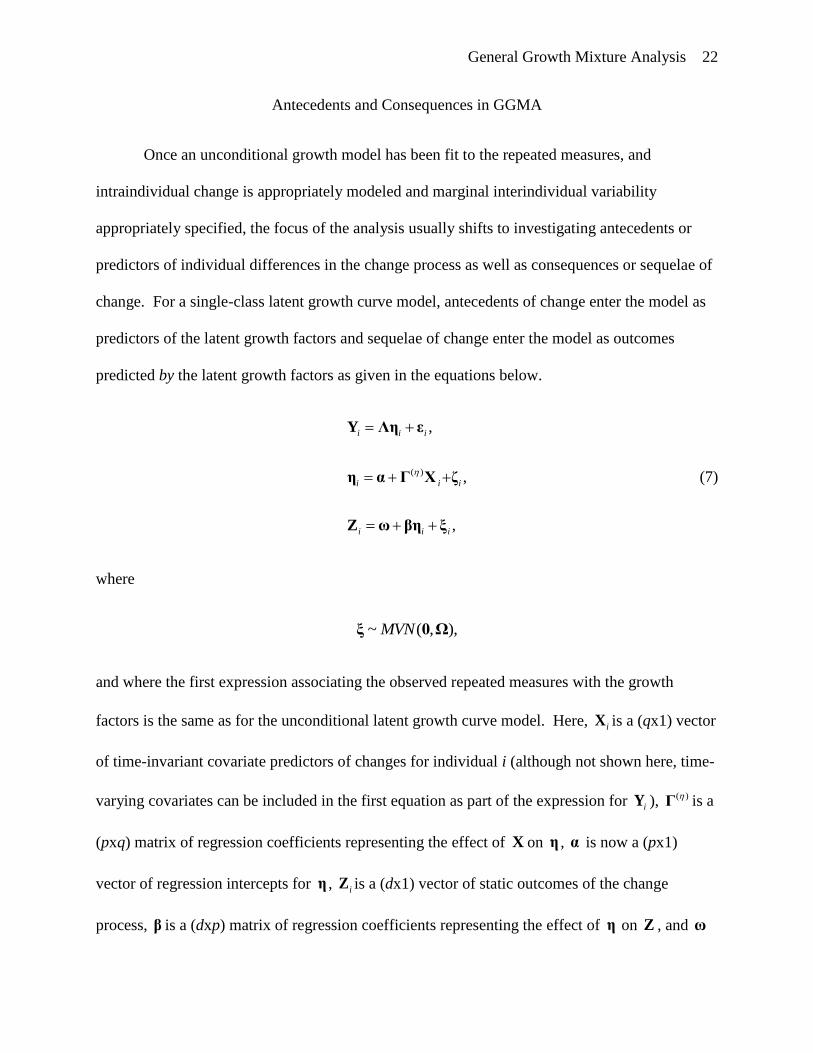
Antecedents and Consequences in GGMA
Once an unconditional growth model has been fit to the repeated measures, and
intraindividual change is appropriately modeled and marginal interindividual variability
appropriately specified, the focus of the analysis usually shifts to investigating antecedents or
predictors of individual differences in the change process as well as consequences or sequelae of
change. For a single-class latent growth curve model, antecedents of change enter the model as
predictors of the latent growth factors and sequelae of change enter the model as outcomes
predicted by the latent growth factors as given in the equations below.
( )
,
,
,
i i i
i i i
i i i
Y Λη ε
η α Γ X ζ
Z ω βη ξ
(7)
where
~ ( , ),MVNξ 0 Ω
and where the first expression associating the observed repeated measures with the growth
factors is the same as for the unconditional latent growth curve model. Here, iX is a (qx1) vector
of time-invariant covariate predictors of changes for individual i (although not shown here, time-
varying covariates can be included in the first equation as part of the expression for iY ), ( )Γ is a
(pxq) matrix of regression coefficients representing the effect of X on η , α is now a (px1)
vector of regression intercepts for η , iZ is a (dx1) vector of static outcomes of the change
process, β is a (dxp) matrix of regression coefficients representing the effect of η on Z , and ω

General Growth Mixture Analysis 23
is a (dx1) vector of regression intercepts for Z . It is possible for the third equation in (7) and the
residual variance/covariance structure of Z to be specified as a generalized linear model to
accommodate not only continuous, but also binary, multinomial, ordinal, and count outcomes of
changes. Notice that similar to the assumption of the unconditional single-class latent growth
curve model that all individuals are drawn from a single population, the conditional model
additionally assumes that predictors have the same influence on the growth factors for all
individuals and that the growth factors have the same influence on subsequent outcomes for all
individuals. Once we shift to a general growth mixture modeling approach, those assumptions
are also relaxed by permitting predictors to influence latent class membership and then having
latent class membership predict to subsequent outcomes. The standard assumptions of additive
linear associations between predictors and growth factors and between growth factors and
outcomes are also relaxed. The integration of antecedents and consequences of latent trajectory
class membership also permit evaluation of the criterion-related validity for mapping the
emergent classes onto theoretical developmental profiles and, ultimately, for evaluating the
validity of the corresponding theory itself. For example, in Moffit’s dual taxonomy, it is
hypothesized that the life course persistent group consists of individuals with deficits in
executive functioning (Moffit, 1993). If the probability of membership in the persistent
trajectory class does not statistically differ in respect to theory driven covariates, such as
executive functioning, then that particular model lacks crucial theoretical support. If there are
repeated failures across various model specifications and samples to find such associations, we
may begin to consider that the theory lacks critical empirical support.
Antecedents

General Growth Mixture Analysis 24
In GGMA, covariates are related to latent trajectory class membership via multinomial logistic
regression, as expressed below.
( )
0
( )
0
1
exp( )Pr( | ) ,
exp( )
C
k k ii i K
C
h h i
h
C k X
Γ X
Γ X
(8)
where Class K is the reference class and 0 0K and ( )C
K Γ 0 for identification. Here, ( )C
kΓ is a
(1xq) vector of logistic regression coefficients representing the effect of X on the log odds of
membership in Class k relative to Class K, and 0k is now the logistic regression intercept for
Class k relative to Class K. These associations between X and C are represented in the path
diagram of Figure 3 by the arrow from X to C.
The set of covariates may also be permitted to influence the within-class interindividual
variability in the change process similar to the associations specified in the second equation of
(7):
( ) ,i k i i
η α Γ X ζ (9)
where ( )Γ is a (pxq) matrix of regression coefficients representing the effect of X on η , and kα
is now a (px1) vector of regression intercepts for η within Class k. These possible associations
are represented in the path diagram of Figure 3 by a dashed arrow from X pointing towards the
growth factors. It is also possible to allow class-specific effects of X onη , that is,
( ) ,i k k i i
η α Γ X ζ (10)

General Growth Mixture Analysis 25
where ( )
k
Γ is a (pxq) matrix of regression coefficients representing the effect of X on η within
Class k, and kα is a (px1) vector of regression intercepts for η within Class k.
There are several critical points to which to pay attention when incorporating covariates
or predictors of change into a growth mixture model. First and foremost, selection and order of
covariate inclusion should follow the same process as with any regular regression model, with
respect to risk factors or predictors of interest, control of potential confounders, etc. Secondly,
although covariates can certainly assist in understanding, interpreting, and assigning meaning to
the resultant classes, i.e., to inform the classes, one should exercise caution if the mixture model
identification is dependent upon the inclusion of covariates or if the formation of the latent
classes is sensitive to the particular subset of covariates included as predictors of class
membership. Based on the simulation work of Nylund and Masyn (2008), misspecification of
covariate effects in a latent class analysis can lead to over-extraction of latent classes more often
than when the latent class enumeration is conducted without covariates. Once the enumeration
process is complete, covariates should first be added to the model only as predictors of the latent
class variable. If the covariates are permitted to influence the change process exclusively
through their effects on class membership in the model and the classes themselves changes
substantively in size or meaning (i.e., the class proportion or class-specific growth parameter
estimates), this can signal a misspecification of the covariate associations with the latent class
indicators. If that occurs, then direct effects, initially class-invariant, from the covariates to the
growth factors themselves should be explored, as given in Equation (9). The covariates should
be centered so that there is not a radical shift in how the centroids of the latent classes are
located, facilitating comparisons in class formation between the unconditional and conditional
models. In the conditional model, the centroids of the latent classes, defined by class-specific

General Growth Mixture Analysis 26
growth factor mean vectors, kα , become the center of growth factor values for the classes at
X 0 . Assuming correct specification of the indirect (via the latent class variable) and direct
effects of the covariates on the growth factors, the resultant classes should align more closely to
the classes obtained from the unconditional growth mixture model. If effects directly from the
covariates to the growth factors are specified in the model, careful consideration should be given
before allowing those effects to be class-varying as well, as in Equation (10). Recall that any
parameter that is permitted to vary across the latent classes becomes an indicator of that latent
class variable. Thus, including class-varying covariate effects on the growth factors results in
latent classes which are defined not only by heterogeneity in growth trajectories but also
heterogeneity in the effect of those covariates on the growth trajectories. This is not an incorrect
model specification, but it does represent what could be a significant departure from the
measurement model originally intended for the latent class variable in the unconditional model.
If the classes continue to change in significant ways relative to the unconditional growth mixture
model with changing subsets of covariates, then careful attention should be paid to the stability
of the model estimation under the original specification and to the solution sensitivity to
covariate inclusion and the entire modeling approach should be reevaluated for data sample at
hand.
Consequences
In addition to including covariates and predictors of change, it is often of interest to relate
the growth trajectories to distal outcomes or sequelae of change (depicted by the arrow from C to
Z and the dashed arrow pointing from η towards Z in Figure 3). This facilitates the assessment
of the predictive power of class membership. While the inclusion of distal outcomes is fairly

General Growth Mixture Analysis 27
straightforward for the single class latent growth curve model, as given in the third equation of
(7), evaluating the associations between growth mixtures and sequelae of change can pose an
analytic dilemma.
There are two primary ways to frame a distal outcome of the change process when a
latent class variable is involved and each way is conceptually and analytically different−the
choice between them is not one that can be made by the data but must be made by the researcher
with understanding of the implications for each alternative. The first way is to treat the distal
outcome(s) as an additional indicator of the latent class variable. The second way is to treat the
latent class variable and distal outcome(s) as a cause-effect pairing such that the distal
outcome(s) is a true consequence of latent class membership.
For the first approach, the indicators for the measurement model of the latent class
variable are made up of the latent growth factors and the distal outcomes (for more, see Muthén
& Shedden, 1999). The latent class variable is characterized by heterogeneity in both the change
process and a later outcome. In other words, the latent class variable captures variability in the
growth factors, variability in the distal outcomes, and the association between the growth factors
and the distal outcomes. In addition to the equations in (5), we add the following to the
measurement model for the latent class variable:
,i k i Z ω ξ (11)
where
~ ( , ).kMVNξ 0 Ω

General Growth Mixture Analysis 28
Here, again, iZ is a (dx1) vector of static outcomes of the change process. kω is a (dx1) vector of
class-specific means for Z given membership in Class k. It is possible for Equation (11) and the
residual variance/covariance structure of Z to be specified as a generalized linear model to
accommodate not only continuous, but also binary, multinomial, ordinal, and count outcomes of
changes. If η and Z are both being used as indicators of the latent class variable, then it may be
desirable to include Z in the class enumeration process since Z would be part of the
measurement model for C. In this case, the residual variance/covariance matrix for Z could be
constrained in a similar way to the one for η , i.e., 1( ,..., )k dDiag Ω , and Z and η , as
indicators for the latent class variable, could be assumed to be conditionally independent given
class membership, i.e., ( , )k kCov Ψ Ω 0 . Although it would be possible to specify and estimate
a regression association within class from η to Z similar to the third equation of (7),
,i k k i i Z ω β η ξ (12)
this would fundamentally change the measurement model for C, where instead of just
including Z as an indicator of C, individual heterogeneity in the association between η and
Z along with the marginal distribution of η would characterize C. Constraining the effect of η
on Z to be class-invariant would reduce the impact of this path on formation of the classes but
be the equivalent of relaxing the conditional independence assumption between η and Z within
class. In either case, with class-varying or class-invariant effects of η on Z , the centroids of the
latent classes on to the scale of Z will be the class-specific means of Z when η 0 .
General Growth Mixture Analysis 29
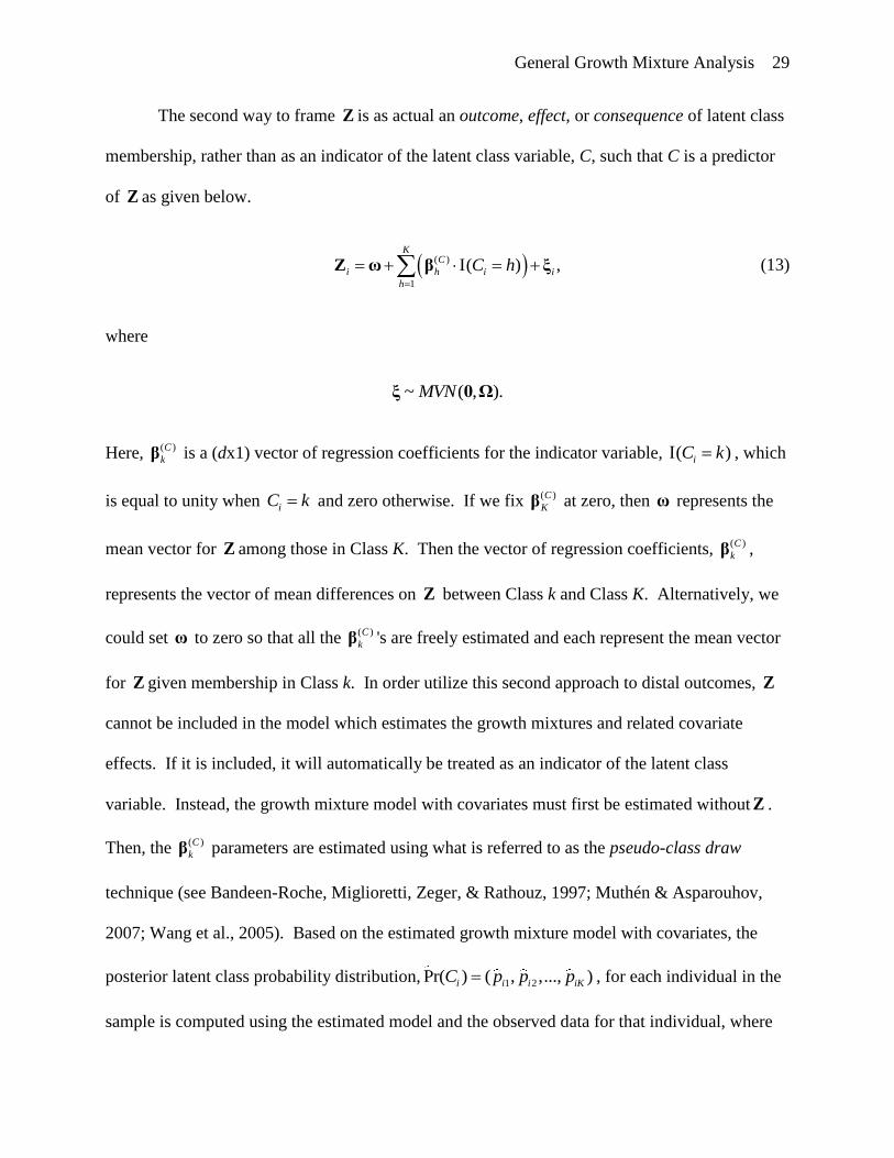
The second way to frame Z is as actual an outcome, effect, or consequence of latent class
membership, rather than as an indicator of the latent class variable, C, such that C is a predictor
of Z as given below.
( )
1
( ) ,K
C
i h i i
h
C h
Z ω β ξ (13)
where
~ ( , ).MVNξ 0 Ω
Here, ( )C
kβ is a (dx1) vector of regression coefficients for the indicator variable, ( )iC k , which
is equal to unity when iC k and zero otherwise. If we fix ( )C
Kβ at zero, then ω represents the
mean vector for Z among those in Class K. Then the vector of regression coefficients, ( )C
kβ ,
represents the vector of mean differences on Z between Class k and Class K. Alternatively, we
could set ω to zero so that all the ( )C
kβ 's are freely estimated and each represent the mean vector
for Z given membership in Class k. In order utilize this second approach to distal outcomes, Z
cannot be included in the model which estimates the growth mixtures and related covariate
effects. If it is included, it will automatically be treated as an indicator of the latent class
variable. Instead, the growth mixture model with covariates must first be estimated without Z .
Then, the ( )C
kβ parameters are estimated using what is referred to as the pseudo-class draw
technique (see Bandeen-Roche, Miglioretti, Zeger, & Rathouz, 1997; Muthén & Asparouhov,
2007; Wang et al., 2005). Based on the estimated growth mixture model with covariates, the
posterior latent class probability distribution, 1 2Pr( ) ( , ,..., )i i i iKC p p p , for each individual in the
sample is computed using the estimated model and the observed data for that individual, where

General Growth Mixture Analysis 30
Pr( )Pr( | , )
Pr( | , ) .Pr( | )
i i i iik i i i
i i
C k C kp C k
Y XY X
Y X (14)
A specified number of random draws, M, are made from the discrete posterior probability distributions
for all individuals in the sample (M=20 is recommended in general, see Wang et al., 2005). For
example, suppose there was an individual with a posterior latent class probability distribution from a
K=3 class growth mixture model computed as 1 2 3Pr( ) ( .80, .15, .05)i i i iC p p p . Pseudo-class
membership for individual i from 20 random draws might look like the following:
1 2 3 4 5 6 7 8 9 10
11 12 13 14 15 16 17 18 19 20
1, 1, 1, 2, 1, 1, 1, 1, 1, 1,
1, 3, 1, 1, 3, 1, 3, 1, 1, 1,
i i i i i i i i i i
i i i i i i i i i i
C C C C C C C C C C
C C C C C C C C C C
where m
iC is the pseudo-class membership for individual i based on random draw m from the
posterior distribution, Pr( )iC . For each pseudo-class draw, the association between Z and C is
estimated using the pseudo-class membership and observed iZ for each individual in the sample;
thus, for Equation (13), we would obtained ( )mC
kβ and mΩ : the estimates for ( )C
kβ and Ω ,
respectively, based on the mth
pseudo-class draw. Consistent estimates for ( )C
kβ are then obtained
by averaging the ( )mC
kβ estimates across the M pseudo-class draws (for proof, see Bandeen-Roche
et al., 1997):
( ) ( )1.
mC C
k k
mM β β (15)
The asymptotic variance of the estimate can be obtained using a similar method to multiple
imputations (described by Rubin, 1987 and Schafer, 1997). Take the simple case with a single
distal outcome of interest, such that d=1 and ( )C
k is a scalar quantity. Suppose that m
kU is the

General Growth Mixture Analysis 31
square of the standard error associated with ( )mC
k . Then the overall square of the standard error
for ( )C
k is given by
1
1 ,W BV V VM
(16)
where WV is the within-imputation (pseudo-class draw) variance of ( )C
k given by
1
,m
W k
m
V UM
and BV is the between-imputation (pseudo-class draw) variance of ( )C
k given by
2
( ) ( )1.
1
mC C
B k k
m
VM
A significance test of the null hypothesis 0k can be performed by comparing the ratio
( )C
k
V
to a Student's t-distribution with degrees of freedom
2
( 1) 1 .( 1)
W
B
MVdf M
M V
In the modeling software, Mplus V5.1 (Muthén & Muthén, 1998-2008), the pseudo-class
draw technique is implemented to perform Wald tests of mean differences on distal outcomes
across the latent classes. A Wald test is performed separately for each outcome variable (for
details, see Muthén & Asparouhov, 2007). However, this pseudo-class draw technique could be

General Growth Mixture Analysis 32
expanded to include multivariate distal outcomes with other observed predictors of the distal
outcomes as well as including the growth factors themselves as predictors in addition to the
latent trajectory class variable, for a more complex model for sequelae of change, as given
below.
( ) ( ) ( )
1
( ) .K
C X
i h i i i i
h
C h
Z ω β I β η β X ξ (17)
We now illustrate the general growth mixture modeling process from class enumeration
to the inclusion of antecedents and distal outcomes of the change process using longitudinal data
from a large population-based randomized trial. All analyses were conducted using the statistical
modeling software, Mplus1, V5.1 (Muthén & Muthén, 1998-2008).
Data Illustration: Development of Aggressive Behavior with Correlates and Consequences
Sample
The data come from a large randomized intervention trial consisting of two cohorts
totaling 2311 students within the 19 participating Baltimore City Public Schools in first grade
(Kellam et al., 2008). Of the population, 1151 (49.8%) were male of which 476 (41.4%) were
assigned to intervention conditions not pertinent to this paper (i.e., Mastery Learning, Good
Behavior Game). Of the remaining 675 control males, 53 (7.9%) had missing values on all
aggression ratings and an additional 7 (1%) had missing values on the covariates. The remaining
sample consisted of 615 male students who did not receive an intervention and who have at least
one valid teacher rating of aggression and no missing values on the covariates. Over 60% of this
sample was African-American (61.6%) and the average age in fall of first grade was 6.3
(SD=0.47).

General Growth Mixture Analysis 33
Longitudinal Outcome
In fall of first grade, teacher reports of child aggressive-disruptive behavior were
gathered twice during first grade and then once per year during second through seventh grade.
The analyses in this chapter focus on the five teacher ratings conducted in spring of first grade to
spring of fifth grade.
Teacher ratings of aggressive-disruptive behavior were obtained using the Teacher
Observation of Classroom Adaptation-Revised (TOCA-R; Werthamer-Larsson et al., 1991). The
TOCA-R is a structured interview with the teacher administered by a trained assessor. The level
of adaptation is rated by teachers on a six-point frequency scale (1=almost never through
6=almost always). The analysis herein used the authority-acceptance subscale which includes the
following items: (1) breaks rules, (2) harms others and property, (3) breaks things, (4) takes
others property, (5) fights, (6) lies, (7) trouble accepting authority, (8) yells at others, (9)
stubborn, and (10) teases classmates. For this chapter, the item-averaged summation scores are
used.
Covariates
For this illustration, two covariates measured in fall of first grade were included in the
analysis: 1) student ethnicity (Black = 1, non-Black = 0) and 2) standardized reading test scores.
The California Achievement Test (CAT, Forms E & F). The CAT represents one of the most
frequently used standardized achievement batteries (Wardrop, 1989). Subtests in CAT-E and F
cover both verbal (reading, spelling, and language) and quantitative topics (computation,
concepts, and applications). Internal consistency coefficients for virtually all of the subscales
exceed .90. Alternate form reliability coefficients are generally in the .80 range (CAT, Forms E

General Growth Mixture Analysis 34
& F). The CAT represents one of the most frequently used standardized achievement batteries
(Wardrop, 1989). Subtests in CAT-E and F cover both verbal (reading, spelling, and language)
and quantitative topics (computation, concepts, and applications). Internal consistency
coefficients for virtually all of the subscales exceed .90. Alternate form reliability coefficients
are generally in the .80 range.
Consequent Outcomes
Records of violent and criminal behavior were obtained at the time of the young adult
follow-up interview and repeated yearly searches were conducted thereafter. The latest search
was conducted in 2007, thus covering adult arrest records up to age 25. Records of incarceration
for an offense classified as a felony in the Uniform Crime Reports system (i.e., armed/unarmed
robbery, assault, kidnapping, weapons, domestic offense, rape/sex offense, attempted murder,
homicide) was used as an indicator of violent and criminal behavior offenses. Drug and property
related offenses (i.e., drug conspiring, distribution, possession, auto theft, burglary, larceny, and
motor vehicle) were coded as non-violent offenses. Violent and nonviolent offenses were then
aggregated over offenses and years such that one or more records of an arrest during that age
range would result in a value of “1” on the nonviolent or the nonviolent crime indicator. These
data were obtained from the Maryland Department of Correction and are considered public
record.
Results
Model Building: Functional Form. Visual inspection of a plot of the sample mean
trajectory shows that, on average, in spring of first grade, males start at a level of 2.2 in
aggressive-disruptive behavior and tend to increase gradually towards an average level of 2.5 in

General Growth Mixture Analysis 35
spring of fifth grade (see Figure 4). Further inspection of individual trajectories makes clear that
there is a tremendous variation around that mean pattern, as is evident by the random subset of
observed individual trajectories plotted in Figure 4. Initial descriptive analysis, as recommended
in the earlier section on model building, suggested that a linear growth model was adequate to
describe intra-individual change across time allowing for fluctuations due to measurement and
time-specific error. Furthermore, a random intercept and a random linear slope had a reasonable
fit to the first and second moments of the current data on the boys’ developmental course of
aggressive-disruptive behavior: 2=20.586, df=10, p=0.0242; CFI=0.981; TLI=0.981;
RMSEA=0.041. (The remaining details of this first step of data screening and descriptive
analyses are omitted in the interest of space.)
Model Building: Class Enumeration
The next step in the model building process is the latent class enumeration. As explained
in detail throughout the first part of this chapter, model specification at this juncture in the
analysis must be purposeful in terms of how the latent classes are to be characterized. In these
analyses, we follow the recommendations given earlier and begin with a set of candidate models
that allow the growth factor means to vary across the latent classes, constrain the growth factor
variances and error variances to be class-invariant, and fix the growth factor covariances and
error covariances to zero within-class. We also need to consider at this point the role of the
distal outcomes in our analysis.
Previously, two alternative latent class measurement model specifications upon which the
class enumeration can performed were described. The first way is to treat the distal outcomes as
additional indicators of the latent class variable and to therefore include the distal outcomes in

General Growth Mixture Analysis 36
the class enumeration process. The second approach treats the distal outcomes as true effects or
consequences of the latent class variable and to therefore exclude them from this step in the
analysis. The results of these two alternative specifications are now described in more detail.
Models with distals-as-class-indicators. In Table 1, the aforementioned fit statistics are
shown for models with an increasing number of classes. There are three 1-class models listed in
the table. The first 1-class model is the independence model for which associations between all
the class indicators, growth factors and distal outcomes are fixed at zero. The second 1-class
model allows the growth factors to co-vary but fixes associations between the distal outcomes
and the distal outcomes with the growth factors to zero. The third 1-class model allows the
growth factors to co-vary, allows the growth factors to associate with the distal outcomes, but
fixes the residual covariance between the distal outcomes to zero. This third and final 1-class
model is the most reasonable single-class baseline model for this class enumeration sequence
since it is the model we would specify if we were working within a conventional latent growth
curve framework and not considering the addition of a latent class variable. Starting with this 1-
class model, the BIC decreased (indicating better fit) towards a 4-class model. However, the
change in the BIC from three to four classes is much smaller than from one to two or from two to
three as is evident by the “elbow” in the top BIC plot of Figure 5. (A proper solution could not
be obtained for a 5-class model without additional constraints, indicating problems with model
identification.) The VLMR-LRT test indicates that a 2-class model can be rejected in favor of a
3-class model (p<.01), while a 3-class model was not rejected in favor of a 4-class model. The
BLRT indicates that a 4-class solution fits superior as compared to a 3-class model. Further
inspection of the estimated mean trajectories reveals that the 4-class solution does not yield a
fourth trajectory class substantively distinct from three trajectory classes derived from the 3-class

General Growth Mixture Analysis 37
solution. Given the small change in BIC, the non-significant VLMR-LRT, and the non-distinct
fourth class, the 3-class solution was selected as the final model to carry forward to the next step
of the analysis.
In the 3-class model (see top plot of Figure 6), the largest class (72%) follows a low-
stable development of aggression, starting at a level of “1.8” in spring of first grade. The two
smaller classes are reasonable comparable in size. One of these classes (16%) starts at a similar
intercept as the low-stable class, but escalates in aggression towards fifth grade. The last class
(12%) starts at a high level of aggressive behavior in spring of first grade followed by a decline
towards fifth grade, which falls below the level of aggressive-disruptive behavior seen for the
low-escalating class.
Models with distals-as-class-consequences. In Table 2, the class enumeration results are
shown for the models without the distal outcomes as additional class indicators. There are two 1-
class models listed in the table. The first 1-class model is the independence model for which the
association between the growth factors is fixed at zero. The second 1-class model allows the
growth factors to co-vary. This second 1-class model is the most reasonable single-class
baseline model for this class enumeration sequence since it is the model we would specify if we
were working within a conventional latent growth curve framework and not considering the
addition of a latent class variable. Starting with this 1-class model the BIC decreased with
additional classes added and reached its lowest value for a 4-class solution. However, the change
in the BIC from three to four classes is somewhat smaller than from one to two or from two to
three as is evident by the “elbow” in the bottom BIC plot of Figure 5. (A proper solution could
not be obtained for a 5-class model without additional constraints, indicating problems with
model identification.) The VLMR-LRT indicates that a 2-class solution can be rejected in favor

General Growth Mixture Analysis 38
of a 3-class solution. The BLRT indicates that a 4-class solution fits superior as compared to a 3-
class model. Further inspection of the estimated mean trajectories reveals that the 4-class
solution does not yield a fourth latent class substantively distinct from three latent classes
derived from the 3-class solution. Given the small change in BIC, the non-significant VLMR-
LRT, and the non-distinct fourth class, the 3-class solution was selected as the final model to
carry forward to the next step of the analysis. As in the first measurement model specification,
the 3-class solution (see bottom plot of Figure 6) yields a low-stable class (72%), a low-
escalating class (15%), and a high-declining class (13%).
When comparing the results of the class enumeration process using the two alternative
measurement model specification, strong similarities regarding the extracted trajectories in terms
of shape and prevalence are found. Additionally, there is very little difference in estimated
within-class growth factor variances: Intercept factor est. SD = 0.45, 0.47; Slope factor est. SD =
0.05, 0.08. We would expect some similarity given the overlap in information on which latent
class formation is based. However, by simply comparing the estimated mean trajectories, we
might incorrectly infer that the latent classes based on the two model specifications are the same
in that the distal outcomes do not contribute to the class characterizations and that class
membership at the individual level is identical across models. Although we do not directly
observe latent class membership, we can explore differences in class membership by comparing
modal class assignment based on the individual posterior class probabilities for each model, as
shown in Table 3. While 94% of individuals assigned to the low-stable trajectory class in at least
one of the models were assigned to that class in both models, only 86% of individuals were
assigned to the high-declining class in both models, and only 54% of individuals for the low-
escalating class. The root of these class formation differences despite the near identical mean

General Growth Mixture Analysis 39
growth trajectories become evident in later section in which we present the class differences with
respect to the distal outcomes.
Predictors of Aggressive-Disruptive Behavior Development
Antecedents of class membership are important to further understand the profile of
individuals in each class as well as to evaluate the criterion-related validity of the latent classes
relative to substantive theory. For this chapter, two covariates measured in fall of first grade
were included. In addition to the students’ ethnicity, the results of a standardized reading test
were used. As suggested by Nylund and Masyn (2008), we first compared the results of the
final unconditional growth mixture model from the class enumeration step to the same model
with the mean-centered covariates included as predictors of class membership, looking for any
evidence of changes in the size and meaning of the classes. While the model results did not
change for either of the three class solutions, the size and meaning of the extracted classes
changed for the four class solutions. This level of instability indicates not only potential model
misspecification of the covariate effects, but also that the three class solution is the preferred
model for this sample. Given the high level of correspondence in class membership for all but
the smallest trajectory class for the two alternative model specifications and the similarity in
mean growth trajectories, it was not surprising to find that the covariate associations to latent
class membership were similar (see Tables 4 and 5). In both cases, Black individuals were
more likely to be in the high-declining and low-escalating classes relative to the low-stable class
compared to non-Black individuals, and individuals with higher reading scores were less likely
to be in the high-declining or low-escalating classes relative to the low-stable class. Neither
covariate distinguished between the high-declining and low-escalating classes in either model.
The most noticeable differences across the models are in the estimated size and significance of

General Growth Mixture Analysis 40
effects of race/ethnicity and reading on membership in the low-escalating class relative to the
low-stable class, with the stronger effects present in the model with distals-as-class-indicators.
Distal Outcomes of Aggressive-Disruptive Behavior Development
A Department of Correction record for a violent or nonviolent crime as an adult is used as
distal outcomes for aggressive-disruptive behavior trajectories in childhood. When including the
distal outcomes in the class enumeration process (see Table 6), the high-declining and low-
escalating classes were both characterized by significantly higher rates of nonviolent and violent
arrests than the low-stable class. Furthermore, the low-escalating class was characterized by
significantly higher rates of nonviolent and violent arrests than the low-escalating class. These
class distinctions are similar (both for pair-wise comparisons and overall comparisons) for each
arrest type.
By comparison, when treating the distal outcomes as consequences of trajectory class
memberships (see Table 7), membership in the high-declining and low-escalating classes is
predictive of higher rates of both nonviolent and violent arrests in adulthood relative to the low-
stable class; however, membership in the low-escalating class is not distinct from membership in
the high-declining class relative to predicted arrest rates. However, similar to the other model,
pair-wise differences due to class membership are similar across arrest type although the overall
effect was stronger for nonviolent that violent arrests.
These disparities between the two model specification help explain why there were
differences in class membership despite the similarity in mean class trajectories. In the model
using the distal outcomes as latent class indicators, individuals placed in the low-escalating
trajectory class were individuals who had both an aggressive-disruptive behavior trajectory

General Growth Mixture Analysis 41
resembling the low-escalating mean trajectory and a high probability of non-violent and violent
arrests. These individuals could very well be those who persist in their higher levels of
aggressive-disruptive behavior into adolescence. For the model in which trajectory classes are
based exclusively on aggressive-disruptive behavior in first through fifth grade, there is not a
high level of predictive validity for adult arrest outcomes beyond that given by any deviation
from the low-stable trajectory pattern, suggesting that information from later childhood and
adolescence may be needed to distinguish arrest risk among those who display non-normative
behavior patterns in middle childhood.
It is important to note here that if we had used the distals-as-class-indicators specification
but then interpreted the model results treating the distal outcomes as effects or consequences of
the trajectory classes, we would have incorrectly infer that individuals in the low-escalating class
were at significantly higher risk for arrest than individuals in the high-declining class. Results
from the distals-as-class-consequences model showed this not to be the case.
Discussion
This chapter has examined the process of including antecedents and consequences of a
developmental process in a growth mixture modeling framework. We have shown that in
addition to the flexibility growth mixture models offer over conventional latent growth curve
models in terms of the way in which population heterogeneity in the growth process itself is
characterized, there is also flexibility gained in terms of how the associations of predictors and
distal outcomes with the growth process are parameterized. We have discussed the
unconditional growth mixture model building process and then demonstrated the addition of
covariates as predictors of the growth process and as possible means for evaluating the

General Growth Mixture Analysis 42
concurrent validity of resultant trajectory classes. We have also presented two different
approaches for including distal outcomes of the growth process. In one approach, the distal
outcomes are included as additional indicators of the latent class variable and, thus, resultant
classes are characterized by individual response patterns on both growth outcomes and distal
outcomes. We noted that if using this approach, one must be careful not to interpret the class-
specific rates of the distal outcome as representing class-predicted patterns but, rather, class-
defining outcome patterns. In the other approach, the distal outcomes are treated as true effects
or consequences of the growth process. The approach offers the possibility of evaluating the
prognostic validity of the resultant trajectory classes. Some recent work has been done to
quantify the predictive validity of trajectory class membership as a screening mechanism for
identifying individuals at-risk for maladaptive distal outcomes using the distal-as-class-indicator
approach (Feldman, Masyn, & Conger, 2008) and this work could be extended to the distal-as-
class-consequence approach. Other work has been done to examine the prediction power of
trajectory class membership in one developmental period for trajectory class membership in a
subsequent development period (see, for example, Boscardin et al., 2008; and for a preventive
intervention settings, see, Petras, Masyn, & Ialongo, 2008) and this work could be extended to
the models presented in this chapter where the earlier latent class variable is treated as an
antecedent or the later latent class variable is treated as a consequence.
There are several interesting areas of investigation for future work. One area involves
extending the distal-as-consequence model to permit more complex models for the distal
outcomes. As specified in this chapter, the distal outcome is assumed to be an observed
univariate or multivariate outcome. However, the distal outcome could itself be a latent variable
with its own measurement model. Another area involved further exploration into the implication

General Growth Mixture Analysis 43
for model specification if the latent trajectory class membership is conceptualized as a time-
invariant attribute at the individual level that merely manifests over time but it is, itself,
independent of time; or if membership is conceptualized as malleable and time-dependent. A
further, and much more complex, matter not dealt with in this chapter, is the collection of the
antecedents, growth process, and consequences as a variable system. In both model approaches
for the distal outcomes, we did not explicitly consider what the implication would be if part of
the shared variance between the growth process and the distal outcomes was due to the
antecedent variables. Confounding of the associations between the growth process and distal
outcomes by the antecedents would have differing impact depending on how the association was
modeled, i.e., distals-as-class-indicators or distals-as-class-consequences. The same is true if the
growth process acted as a mediator of the antecedent effect on the distal outcome or if the
antecedents acted as moderators of the associations between the growth process and the distal
outcomes.
Clearly, these models hold great potential for aiding empirical investigations of
developmental theories of normative and non-normative behaviors and maladaptive outcomes
across the lifespan. In no way is this more evident than in the marked increase in their use
among applied researchers in criminology and other behavioral sciences. We maintain, as
expounded at the beginning of this chapter, that the value and future potential of these models for
examining population heterogeneity in developmental processes and correlates thereof, holds
regardless of whether the resultant latent trajectory classes represent "true" subpopulations or
simply reflect non-normality in the population distribution of the growth factors. However, there
is still much opportunity in the realm of methods development to capitalize on the potential of
these models and extensions to better accommodate the complexities or our developmental

General Growth Mixture Analysis 44
theories. And, as with any statistical tool, the research question along with previous theoretical
and empirical work, should guide these models’ application in a particular study, with thoughtful
and purposeful choices for model specification, selection, and interpretation.

General Growth Mixture Analysis 45
References
Bandeen-Roche, K., Miglioretti, D.L., Zeger, S.L., & Rathouz, P.J. (1997). Latent variable
regression for multiple discrete outcomes. Journal of the American Statistical
Association, 92(440), 1375-1386.
Bauer, D.J., & Curran, P.J. (2003). Distributional assumptions of growth mixture models:
Implications for overextraction of latent trajectory classes. Psychological Methods, 8,
338-363.
Bauer, D.J., & Curran, P.J. (2004). The integration of continuous and discrete latent variable
models: Potential problems and promising opportunities. Psychological Methods, 9, 3-29.
Bollen, K.A., & Curran, P.J. (2006). Latent curve models: A structural equation perspective.
Hoboken, NJ: John Wiley & Sons, Inc.
Boscardin, C., Muthén, B., Francis, D., & Baker, E. (2008). Early identification of reading
difficulties using heterogeneous developmental trajectories. Journal of Educational
Psychology, 100, 192-208.
Broidy, L.M., Nagin, D. S., Tremblay, R. E., Bates, J. E., Brame, B., Dodge, K. A., Fergusson,
D., Horwood, J.L., Loeber, R., Laird, R., Lyman, D.R., Moffitt, T. E., Pettit, G.S., &
Vitaro, F. (2003). Developmental trajectories of childhood disruptive behaviors and
adolescent delinquency: A six-site, cross-national study. Developmental Psychology, 39,
222-245.
Bushway, S.D., Brame, R., & Paternoster, R.E. (1999). Assessing stability and change in
criminal offending: A comparison of random effects, semiparametric, and fixed effects
modeling strategies. Journal of Quantitative Criminology, 15, 23-61.

General Growth Mixture Analysis 46
Duncan, T.E., Duncan, S.C., & Strycker, L.A. (2006). An introduction to latent variable growth
curve modeling: Concepts, issues, and applications (2nd ed.). Mahwah, NJ: Lawrence
Erlbaum Associates.
Ensminger, M.E, Kellam, S.G, & Rubin, B.R. (1983), School and family origins of delinquency:
Comparisons by sex. In: Van Dusen KT, Mednick SA (eds.,) Prospective Studies of
Crime and Delinquency (pp. 73-97). Boston: Kluwer-Niejhoff.
Feldman, B., Masyn, K., and Conger, R. (2008). Assessing the quality of prediction from
adolescent problem-behavior trajectories to distal categorical outcomes. Manuscript
submitted for publication.
Hawkins, J.D., Herrenkohl, T.I., Farrington, D.P., Brewer, D., Catalano, R.F., Harachi, T.W., &
Cothern, L. (2000), Predictors of youth violence. Office of Juvenile Justice and
Delinquency Prevention Bulletin, 4, 1-11.
Heckman J., & Singer, B. (1984) A method for minimizing the distributional assumptions in
econometric models for duration data. Econometrica, 52, 271-320.
Hedecker, D. & Gibbons, R.D. (2008). Supermix – Mixed Effects Models. Chicago:
Scientific Software International.
Hipp, J. R., & Bauer, D. J. (2006). Local solutions in the estimation of growth mixture models.
Psychological Methods, 11(1), 36-53.
Hox, J.J. (2000). Multilevel analysis of grouped and longitudinal data. In: T.D. Little, K.U.
Schnabel & J. Baumert (Eds.). Modeling longitudinal and multiple-group data. Practical
issues, applied approaches, and specific examples. Hillsdale, NJ: Lawrence Erlbaum.
Hox, J.J. (2002). Multilevel Analysis. Techniques and Applications. Mahwah, NJ: Lawrence
Erlbaum Associates.

General Growth Mixture Analysis 47
Hu, L., & Bentler, P. (1999). Cutoff criteria for fit indexes in covariance structure analysis:
Conventional criteria versus new alternatives. Structural Equation Modeling, 6(1), 1-55.
Jones, B.L., Nagin, D.S., & Roeder, K. (2001). A SAS procedure based on mixture models for
estimating developmental trajectories. Sociological Methods & Research, 29, 374–393.
Jöreskog, K.G. & Sörbom, D. (1996). LISREL 8: Structural Equation Modeling. Chicago:
Scientific Software International.
Kellam, S.G., Brown, C.H., Poduska, J.M, Ialongo, N.S., Wang, W., Toyinbo, P., Petras, H.,
Ford, C., Windham, A., & Wilcox, H.C. (2008). Effects of a universal classroom
behavior management program in first and second grades on young adult behavioral,
psychiatric, and social outcomes. Drug and Alcohol Dependence, 95, S5-S28.
Kreuter, F., & Muthén, B. (2007). Longitudinal modeling of population heterogeneity;
Methodological challenges to the analysis of empirically derived criminal trajectory
profiles. In G. R. Hancock, & Samuelsen, K. M. (Ed.), Advances in latent variable
mixture models. Charlotte, NC: Information Age Publishing.
Kreuter, F., & Muthén, B. (2008). Analyzing criminal trajectory profiles: Bridging multilevel
and group-based approaches using growth mixture modeling. Journal of Quantitative
Criminology, 24, 1-31.
Lo, Y., Mendell, N., & Rubin, D. (2001). Testing the number of components in a normal
mixture. Biometrika, 88, 767-778.
Loeber, R., & Hay, D. (1997). Key issues in the development of aggression and violence from
childhood to early adulthood. Annual Review of Psychology, 48, 371-410.
Lubke, G. H., & Spies, J. R. (2008). Choosing a "correct" factor mixture model: Power,
limitations, and graphical data exploration. In G. R. Hancock & K. M. Samuelson (Eds.),

General Growth Mixture Analysis 48
Advances in latent variable mixture models (pp. 343-361). Charlotte, NC: Information
Age Publishing.
Lynam, D.R. (1996), The early identification of chronic offenders: Who is the fledging
psychopath? Psychological Bulletin, 120, 209-234.
Magnusson, D. (1998). The logic and implications of a person-oriented approach. In R. B.
Cairns, L. R. Bergman, & J. Kagan (Eds.), Methods and models for studying the
individual (pp. 33-64). Thousand Oaks, CA: Sage.
Maughan, B., & Rutter, M. (1998). Continuities and discontinuities in antisocial behavior from
childhood to adult life. In T. H. Ollendick & R. J. Prinz (Eds.), Advances in Clinical
Child Psychology, Vol. 20 (pp. 1-47). New York: Plenum.
McCord, J., & Ensminger, M.E. (1997), Multiple risks and co-morbidity in an African-American
population. Criminal Behavior and Mental Health, 7, 339-352.
McLachlan, G., & Peel, D. (2000). Finite mixture models. New York: Wiley.
Meredith, W., & Tisak, J. (1990). Latent curve analysis. Psychometrika, 55, 107–22
Moffitt, T. E. (1993). Adolescent-limited and life-course persistent antisocial behavior: A
developmental taxonomy. Psychological Review, 100, 674-701.
Muthén, B. (2000). Methodological issues in random coefficient growth modeling using a latent
variable framework: Applications to the development of heavy drinking in ages 18-37.
In J. S. Rose, L. Chassin, C. Presson, & J. Sherman (Eds.), Multivariate applications in
substance use research: New methods for new questions (pp. 113-140). Mahwah, NJ:
Erlbaum.
Muthén, B. (2001). Second-generation structural equation modeling with a combination of
categorical and continuous latent variables: New opportunities for latent class/latent

General Growth Mixture Analysis 49
growth modeling. In Collins, L.M. & Sayer, A. (eds.), New Methods for the Analysis of
Change (pp. 291-322). Washington, D.C.: APA.
Muthén, B. (2003). Statistical and substantive checking in growth mixture modeling.
Psychological Methods, 8, 369-377.
Muthén, B. (2004). Latent variable analysis: Growth mixture modeling and related techniques
for longitudinal data. In: Kaplan, D. (Ed.), Handbook of Quantitative Methodology for
the Social Sciences (pp. 345-368). Sage, Newbury Park, CA.
Muthén, B. (2006). The potential of growth mixture modeling. Commentary. Infant and Child
Development, 15, 623–625
Muthén, B., & Asparouhov, T. (2008). Growth mixture modeling: Analysis with non-Gaussian
random effects. In: Fitzmaurice, G., Davidian, M., Verbeke, G., Molenberghs, G. (Eds.),
Longitudinal Data Analysis (143-165). Boca Raton: Chapman & Hall/CRC Press.
Muthén, B., & Asparouhov, T. (2007). Wald test of mean equality for potential latent class
predictors in mixture modeling. (Unpublished Web Note). http://www.statmodel.com.
Muthén, B., Brown, C.H., Masyn, K., Jo, B., Khoo, S.T., Yang, C.C., Wang, C.P., Kellam, S.,
Carlin, J., & Liao, J. (2002). General growth mixture modeling for randomized
preventive interventions. Biostatistics, 3, 459-475.
Muthén, B.O., & Curran, P.J. (1997). General longitudinal modeling of individual differences in
experimental designs: A latent variable framework for analysis and power estimation.
Psychological Methods, 2, 371-402.
Muthén, B., & Muthén, L. K. (2000). Integrating person-centered and variable-centered
analyses: Growth mixture modeling with latent trajectory classes. Alcoholism: Clinical
and Experimental Research, 24, 1 –10.

General Growth Mixture Analysis 50
Muthén, B.O., & Muthén, L.K. (2000). The development of heavy drinking and alcohol-related
problems from ages 18 to 37 in a U. S. national sample. J. Stud. Alcohol, 61, 290-300.
Muthén, B., & Muthén, L. K. (1998 - 2008). Mplus (Version 5.1) [Computer software]. Los
Angeles, CA: Muthén & Muthén.
Muthén, L. K., & Muthén, B. (1998-2008). Mplus user's guide (5th ed.). Los Angeles: Muthén &
Muthén.
Muthén, B., & Shedden, K. (1999). Finite mixture modeling with mixture outcomes using the
EM algorithm. Biometrics, 6, 463-469.
Nagin, D. S. (1999). Analyzing developmental trajectories: A semiparametric, group-based
approach. Psychological Methods, 4, 139-157.
Nagin, D. S., & Land, K. C. (1993). Age, criminal careers, and population heterogeneity:
Specification and estimation of a nonparametric, mixed Poisson model. Criminology, 31,
327-362.
Nagin, D., & Tremblay, R. E. (1999). Trajectories of boys’ physical aggression, opposition, and
hyperactivity on the path to physically violent and nonviolent juvenile delinquency.
Child Development, 70, 1181-1196.
Nagin, D. S., & Tremblay, R. (2005). Developmental trajectory groups: Fact or a useful
statistical fiction? Criminology, 43(4), 873–903.
Nagin, D. (2005). Group-based modeling of development. Harvard University Press: Cambridge,
Massachusetts.
Nylund, K.L., Asparouhov, T., & Muthén, B. (2007). Deciding on the number of classes in latent
class analysis and growth mixture modeling: A Monte Carlo simulation study. Structural
Equation Modeling, 14, 535-569.

General Growth Mixture Analysis 51
Nylund, K. L., & Masyn, K. E. (2008). Covariates and latent class analysis: Results of a
simulation study. Paper presented at the Society for Prevention Research Annual
Meeting.
Patterson, G. R., DeBaryshe, B. D., & Ramsey, E. (1989). A developmental perspective on
antisocial behavior. American Psychologist, 44, 329-335.
Patterson, G. R., Forgatch, M. S., Yoerger, K. L., & Stoolmiller, M. (1998). Variables that
initiate and maintain an early-onset trajectory for juvenile offending. Development and
Psychopathology, 10, 531-547.
Petras, H., Schaeffer, C.M., Ialongo, N., Hubbard, S., Muthen, B., Lambert, S., Poduska, J., &
Kellam, S. (2004). When the course of aggressive behavior in childhood does not predict
antisocial behavior: An examination of potential explanatory variables. Development and
Psychopathology, 16, 919-941.
Petras, H., Kellam, S.G., Brown, H., Muthén, B., Ialongo, N. & Poduska, J.M.. (2008).
Developmental epidemiological courses leading to antisocial personality disorder and
violent and criminal behavior: Effects by young adulthood of a universal preventive
intervention in first- and second-grade classrooms. Drug and Alcohol Dependence, 95,
S45-S59.
Petras, H., Masyn, K., & Ialongo, N. (2008). The distal impact of two first-grade preventive
interventions on aggressive disruptive behavior in adolescence – An application of a
latent transition hybrid model. Manuscript in preparation.
Picquero, A. (2008). Taking stock of developmental trajectories of criminal activity over the life
course. In: Akiva M. Liberman (Ed.). The long view of crime: A synthesis of longitudinal
Research, (p23-70). Springer Publication.

General Growth Mixture Analysis 52
Rabe-Hesketh, S., Skrondal, A. and Pickles, A. (2004). GLLAMM Manual. U.C. Berkeley
Division of Biostatistics Working Paper Series. Working Paper 160.
Rasbash, J., Steele, F., Browne, W., and Prosser, B.(2004). A user's guide to MLwiN version 2.0.
London, Institute of Education.
Ramaswamy, V., Desarbo, W. S., Reibstein, D. J., & Robinson, W. T. (1993). An empirical
pooling approach for estimating marketing mix elasticities with PIMS data. Marketing
Science, 12(1), 103-124.
Raudenbush, S.W., & Bryk, A.S. (2002). Hierarchical Linear Models: Applications
and Data Analysis Methods(2nd ed.). Sage Publications, Newbury Park, CA.
Raudenbush, S.W., Bryk, A.S., Cheong, Y., & Congdon, R. (2000). HLM 5: Hierarchical
Linear and Nonlinear Modeling . Chicago: Scientific Software International.
Roeder, K. Lynch, K.G., & Nagin, D.S. (1999). Modeling uncertainty in latent class
membership: A case study in criminology. Journal of the American Statistical
Association, 94, 766–776.
Rubin, D.B. (1987). Multiple imputation for nonresponse in surveys. New York: J. Wiley &
Sons.
Sampson, R., & Laub, J. (2003). Life-course desisters? Trajectories of crime among delinquent
boys followed to age 70. Criminology, 41, 555-592.
Sampson, R.J., & Laub, J. (2005). Seductions of methods: Rejoinder to Nagin & Tremblay’s
Developmental Trajectory Groups: Fact or Fiction? Criminology, 43, 905-914.
Sampson, R.J., Laub, J., & Eggleston, E.P. (2004). On the robustness and validity of groups.
Journal of Quantitative Criminology, 20, 37-42.
Schaeffer, C.M., Petras, H., Ialongo, N., Masyn, K.E., Hubbard, S., Poduska, J., &

General Growth Mixture Analysis 53
Kellam, S. (2006). A comparison of girls' and boys' aggressive-disruptive behavior
trajectories across elementary school: prediction to young adult antisocial outcomes.
Journal of Consulting and Clinical Psychology. 74, 500-510.
Shaw, D. S., Gilliom, M., Ingoldsby, E.M., & Nagin, D. S. (2003). Trajectories leading to
school-age conduct problems. Developmental Psychology, 39, 189-200.
Schafer, J.L. (1997). Analysis of incomplete multivariate data. London: Chapman & Hall.
Schwarz, G. (1978). Estimating the dimension of a model. The Annals of Statistics, 6, 461-464.
Singer, J.D., & Willett, J.B. (2003). Applied longitudinal data analysis. New York: Oxford
University Press.
Stram, D.O., & Lee, J.W. (1994). Variance components testing in the longitudinal mixed effects
model. Biometrics, 40, 961-971.
Thorndike, R. L. (1953). Who belong in the family? Psychometrika, 18(4), 267-276.
van Dulmen, M. H. M., Goncy, E., Vest, A., & Flannery, D. J. (in press). Group based trajectory
modeling of externalizing behavior problems from childhood through adulthood:
Exploring discrepancies in empirical findings. In J. Savage (Ed.), The development of
persistent criminality. New York, NY: Oxford University Press.
Vermunt, J. K., & Magidson, J. (2002). Latent class cluster analysis. In J. A. Hagenaars & A. L.
McCutcheon (Eds.), Applied latent class analysis (pp. 89-106). Cambridge: Cambridge
University Press.
Vermunt, J.K. & Magidson, J. (2005). Technical Guide for Latent GOLD 4.0: Basic and
Advanced. Belmont Massachusetts: Statistical Innovations Inc.
Wang, C-P., Brown, C.H., & Bandeen-Roche, K. (2005). Residual diagnostics for growth
mixture models: Examining the impact of a preventive intervention on multiple

General Growth Mixture Analysis 54
trajectories of aggressive behavior. Journal of the American Statistical Association,
100(3), 1054-1076.
Wardrop, J. L. (1989). Review of the California Achievement Tests, Forms E and F. In J. Close
Conoley & J. Kramer(Eds.), The tenth mental measurements yearbook(pp. 128–133),
Lincoln: University of Nebraska Press.
Werthamer-Larsson, L., Kellam, S. G., & Wheeler, L. (1991). Effect of first-grade classroom
environment on child shy behavior, aggressive behavior, and concentration problems.
American Journal of Community Psychology, 19, 585-602.
Willett, J.B., & Sayer, A.G. (1994). Using covariance structure analysis to detect correlates and
predictors of individual change over time. Psychological Bulletin, 116, 363–81
Yoshikawa, H. (1994). Prevention as cumulative protection: Effects of early family support and
education on chronic delinquency and its risks. Psychological Bulletin, 115, 28-54.

General Growth Mixture Analysis 55
Footnotes
1 Although we chose to use the Mplus modeling software, there are other software packages that
can be used to estimated some (or all) of the models presented herein. Among the most
prominent are: HLM (Raudenbush, Bryk, Cheong, & Congdon, 2000); SAS Proc TRAJ (Jones,
Nagin, & Roeder, 2001); GLAMM (Rabe-Hesketh, Skrondal, & Pickles, 2004); MLwiN
(Rasbash, Steele, Browne, & Prosser, 2004); Latent Gold (Vermunt & Magidson, 2005);
SuperMix (Hedecker & Gibbons, 2008); and LISREL (Jöreskog & Sörbom, 1996).
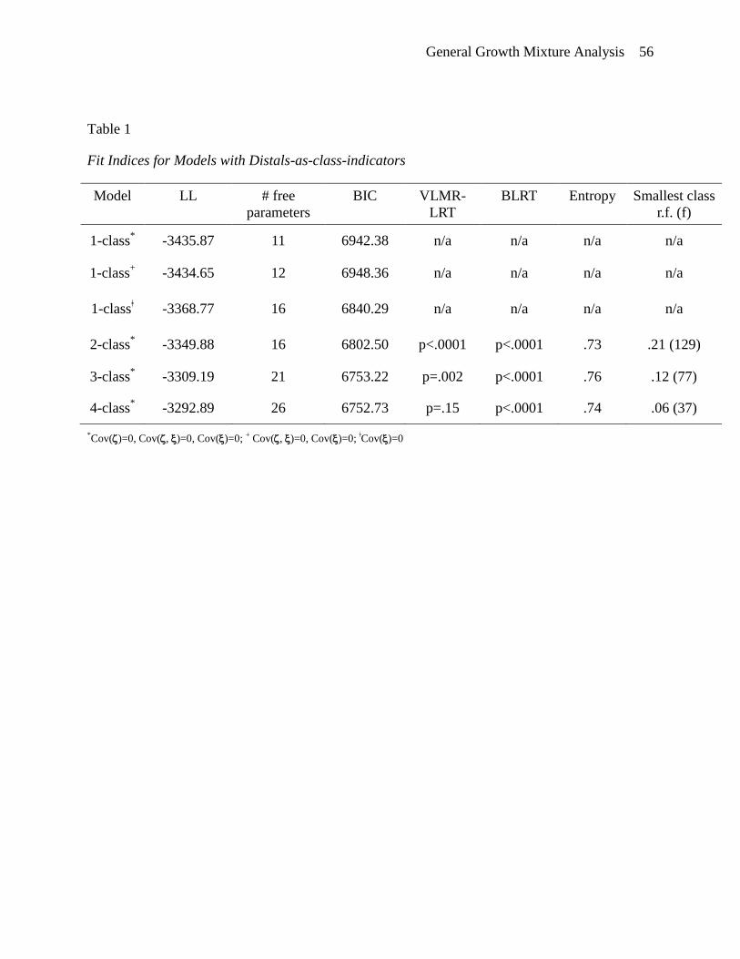
General Growth Mixture Analysis 56
Table 1
Fit Indices for Models with Distals-as-class-indicators
Model LL # free
parameters BIC VLMR-
LRT BLRT Entropy Smallest class
r.f. (f)
1-class*
-3435.87 11 6942.38 n/a n/a n/a n/a
1-class+
-3434.65 12 6948.36 n/a n/a n/a n/a
1-classǂ -3368.77 16 6840.29 n/a n/a n/a n/a
2-class* -3349.88 16 6802.50 p<.0001 p<.0001 .73 .21 (129)
3-class* -3309.19 21 6753.22 p=.002 p<.0001 .76 .12 (77)
4-class* -3292.89 26 6752.73 p=.15 p<.0001 .74 .06 (37)
*Cov()=0, Cov(, )=0, Cov()=0; + Cov(, )=0, Cov()=0; ǂCov()=0
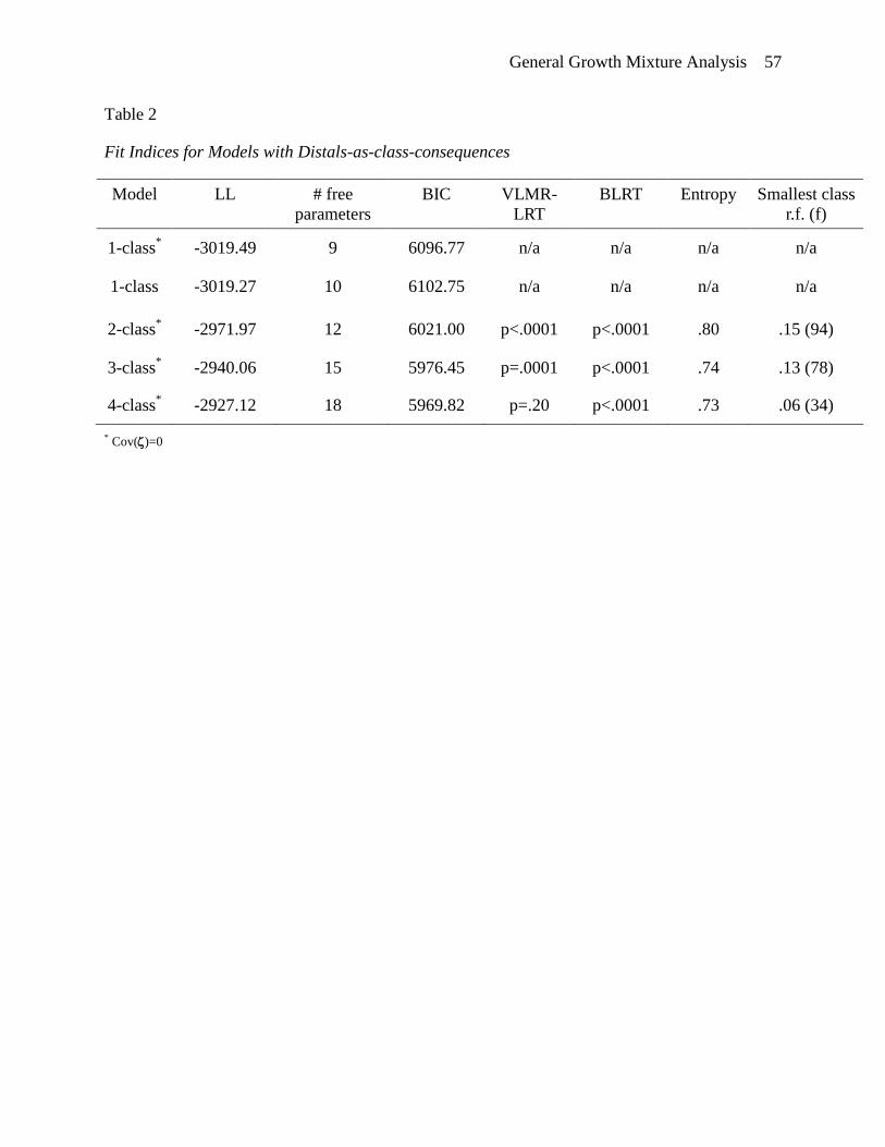
General Growth Mixture Analysis 57
Table 2
Fit Indices for Models with Distals-as-class-consequences
Model LL # free
parameters BIC VLMR-
LRT BLRT Entropy Smallest class
r.f. (f)
1-class*
-3019.49 9 6096.77 n/a n/a n/a n/a
1-class -3019.27 10 6102.75 n/a n/a n/a n/a
2-class* -2971.97 12 6021.00 p<.0001 p<.0001 .80 .15 (94)
3-class* -2940.06 15 5976.45 p=.0001 p<.0001 .74 .13 (78)
4-class* -2927.12 18 5969.82 p=.20 p<.0001 .73 .06 (34)
* Cov()=0

General Growth Mixture Analysis 58
Table 3
Cross-tabulation of Modal Latent Class Assignment based on Model with Distals-as-class-
indicators versus Distals-as-class-consequences
Distals-as-class-consequences
Low-Stable High-Declining Low-Escalating Total
Distals-as-
class-indicators
Low-Stable 442 6 20 468
High-Declining 1 66 2 69
Low-Escalating 22 2 54 78
Total 465 74 76 615

General Growth Mixture Analysis 59
Table 4
Latent Class Multinomial Regression Results for 3-Class Model with Distals-as-class-indicators
Covariate Target Class Reference Class Est. S.E. p-value Est. OR*
Race/Ethnicity
High-Declining
Low-Stable 0.90 0.36 .01 2.46
+
Low-Escalating 1.27 0.43 .004 3.56+
High-Declining Low-Escalating -0.37 0.55 .51 0.69+
Reading
High-Declining
Low-Stable -0.01 0.004 <.001 0.67
ǂ
Low-Escalating -0.01 0.004 .001 0.67ǂ
High-Declining Low-Escalating 0.001 0.01 .89 1.04ǂ
*Odds (membership in target class) : Odds (membership in reference class) among individuals in either target or reference class +Calculated for Ethnicity = Black vs. Ethnicity = Non-Black
ǂ Calculated for a 1 SD increase in reading score
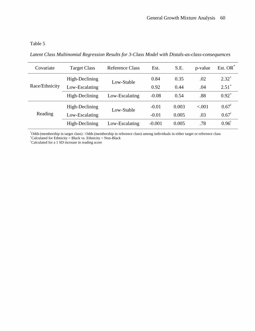
General Growth Mixture Analysis 60
Table 5
Latent Class Multinomial Regression Results for 3-Class Model with Distals-as-class-consequences
Covariate Target Class Reference Class Est. S.E. p-value Est. OR*
Race/Ethnicity
High-Declining
Low-Stable 0.84 0.35 .02 2.32
+
Low-Escalating 0.92 0.44 .04 2.51+
High-Declining Low-Escalating -0.08 0.54 .88 0.92+
Reading
High-Declining
Low-Stable -0.01 0.003 <.001 0.67
ǂ
Low-Escalating -0.01 0.005 .03 0.67ǂ
High-Declining Low-Escalating -0.001 0.005 .78 0.96ǂ
*Odds (membership in target class) : Odds (membership in reference class) among individuals in either target or reference class +Calculated for Ethnicity = Black vs. Ethnicity = Non-Black
ǂ Calculated for a 1 SD increase in reading score
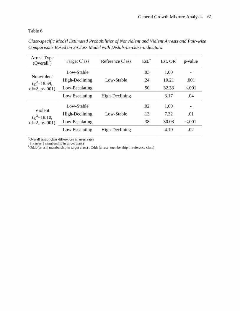
General Growth Mixture Analysis 61
Table 6
Class-specific Model Estimated Probabilities of Nonviolent and Violent Arrests and Pair-wise
Comparisons Based on 3-Class Model with Distals-as-class-indicators
Arrest Type
(Overall*) Target Class Reference Class Est.
+ Est. OR
ǂ p-value
Nonviolent
(2=18.69,
df=2, p<.001)
Low-Stable
Low-Stable
.03 1.00 -
High-Declining .24 10.21 .001
Low-Escalating .50 32.33 <.001
Low Escalating High-Declining 3.17 .04
Violent
(2=18.10,
df=2, p<.001)
Low-Stable
Low-Stable
.02 1.00 -
High-Declining .13 7.32 .01
Low-Escalating .38 30.03 <.001
Low Escalating High-Declining 4.10 .02
*Overall test of class differences in arrest rates +Pr (arrest | membership in target class) ǂ Odds (arrest | membership in target class) : Odds (arrest | membership in reference class)
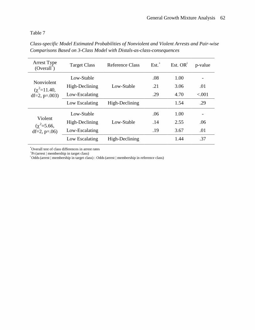
General Growth Mixture Analysis 62
Table 7
Class-specific Model Estimated Probabilities of Nonviolent and Violent Arrests and Pair-wise
Comparisons Based on 3-Class Model with Distals-as-class-consequences
Arrest Type
(Overall*)
Target Class Reference Class Est.+
Est. ORǂ
p-value
Nonviolent
(2=11.40,
df=2, p=.003)
Low-Stable
Low-Stable
.08 1.00 -
High-Declining .21 3.06 .01
Low-Escalating .29 4.70 <.001
Low Escalating High-Declining 1.54 .29
Violent
(2=5.66,
df=2, p=.06)
Low-Stable
Low-Stable
.06 1.00 -
High-Declining .14 2.55 .06
Low-Escalating .19 3.67 .01
Low Escalating High-Declining 1.44 .37
*Overall test of class differences in arrest rates +Pr (arrest | membership in target class) ǂ Odds (arrest | membership in target class) : Odds (arrest | membership in reference class)

General Growth Mixture Analysis 63
Figure Captions
Figure 1. Path diagram for an unconditional linear latent growth curve model. Model is shown
with fixed times of measurement, but individually-varying times of measurement may be
specified.
Figure 2. Illustration of a finite mixture of two normally-distributed subpopulations (dashed
lines) and the resultant mixed population distribution (solid line).
Figure 3. Path diagram for a general (linear) growth mixture model with observed static
antecedents (X) and consequences (Z) of change.
Figure 4. Sample average trajectory (bolded) and observed individual trajectories (random
subset, n=25)
Figure 5. BIC “elbow” plots for models with distals-as-class-indicators (top) and with distals-as-
class-consequences (bottom).
Figure 6. Model-estimated class-specific mean growth trajectory plots based on 3-class model
with distals-as-class-indicators (top) and 3-class model with distals-as-class-consequences
(bottom).
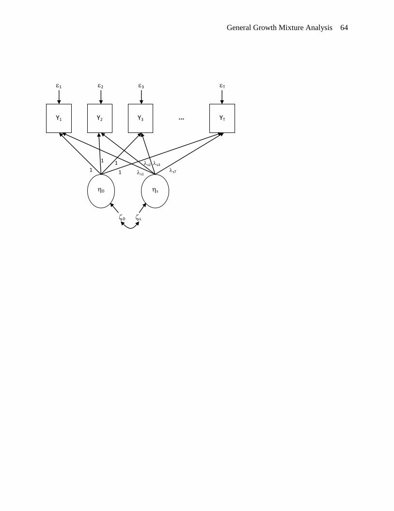
General Growth Mixture Analysis 64
1
T 3 2 1
YT
...
Y3
Y2
Y1
s3 s2
s1 sT 1
1 1
s
0
0 s
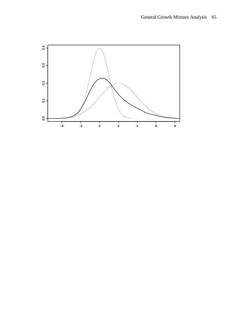
General Growth Mixture Analysis 65
-4 -2 0 2 4 6 8
0.0
0.1
0.2
0.3
0.4
-4 -2 0 2 4 6 8
0.0
0.1
0.2
0.3
0.4
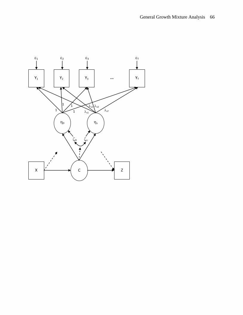
General Growth Mixture Analysis 66
Z
X
1
T 3 2 1
YT
...
Y3
Y2
Y1
s3 s2
s1 sT 1
1 1
C
s
0
0 s
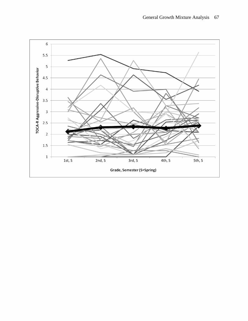
General Growth Mixture Analysis 67
5th, S 2nd, S 3rd, S 4th, S 1st, S
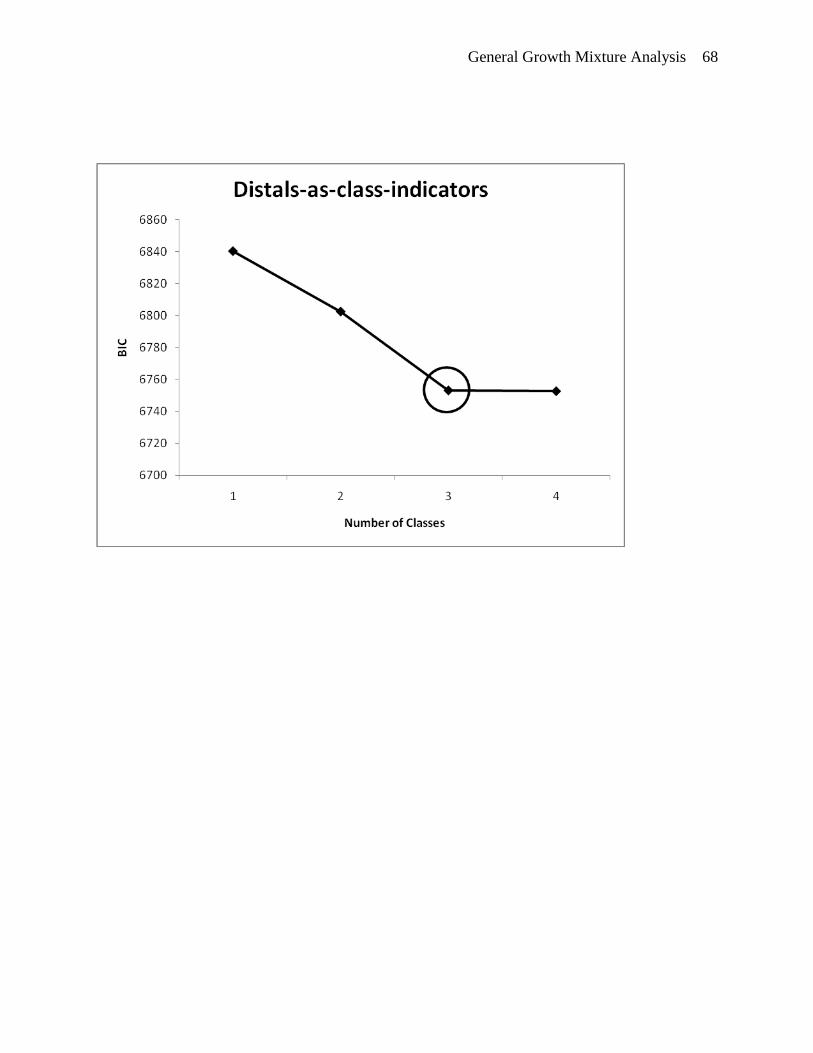
General Growth Mixture Analysis 68
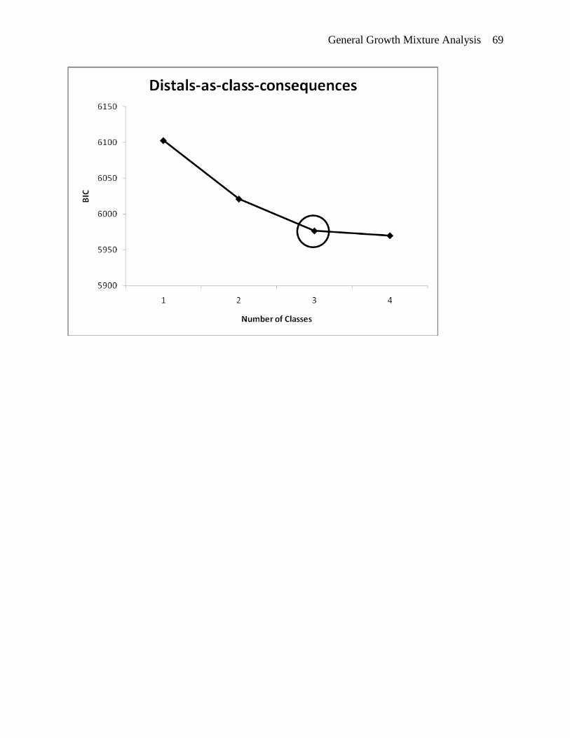
General Growth Mixture Analysis 69

General Growth Mixture Analysis 70
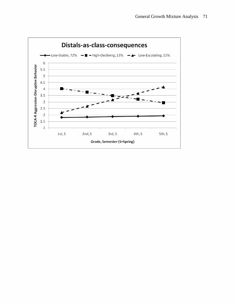
General Growth Mixture Analysis 71