Embed Size (px)
Citation preview
Gauging the Military Value ofNaval Infrastructure
A. I. Kaufman, Project LeaderE. Zdankiewicz
I N S T I T U T E F O R D E F E N S E A N A L Y S E S
IDA Paper P-3605
Log: H 01-000666
March 2001
Approved for public release;distribution unlimited.

This work was conducted under contract DASW01 98 C 0067, TaskAB-1-1680, for OUSD(AT&L), Deputy Director of Naval Warfare and theHead of the Manpower, Personnel, Training, Education and InfrastructureBranch (N813) in the Office of the Deputy Chief of Naval Operations forResources, Warfare Requirements & Assessment (N8). The publicationof this IDA document does not indicate endorsement by the Department ofDefense, nor should the contents be construed as reflecting the officialposition of that Agency.
© 2001 Institute for Defense Analyses, 1801 N. Beauregard Street, Alexandria, Virginia 22311-1772 • (703) 845-2000.
This material may be reproduced by or for the U.S. Government pursuantto the copyright license under the clause at DFARS 252.227-7013(NOV 95).

I N S T I T U T E F O R D E F E N S E A N A L Y S E S
IDA Paper P-3605
Gauging the Military Value ofNaval Infrastructure
A. I. Kaufman, Project LeaderE. Zdankiewicz

UNCLASSIFIED
UNCLASSIFIED
iii
PREFACE
In this paper we accomplish three things. First, we fill a gap in the analytic capability available to the Department of Defense by proposing a methodology for quantitatively connecting changes in naval infrastructure to the corresponding changes in warfare capability. Second, we show that this methodology can be executed by applying it to an organic mine countermeasure operation. Finally, we show that the recommended methodology offers a straightforward way of rank-ordering alternative investments in order of their relative cost-effectiveness by applying it to a specific decision between two alternatives in a shallow water antisubmarine warfare operation.
The foundation of our methodology is a new definition of infrastructure, one that emphasizes its natural connection to warfare. Specifically, we suggest that infrastructure is the totality of all people, facilities, and activities designed to produce a structure able to operate as desired, now as well as in the indefinite future, and which fulfills the function assigned to it. Hence, each element of naval structure has a double character. On the one hand, they directly participate in war and thereby contribute directly to warfare capability; on the other, they are also products of naval infrastructure and thereby reflect the quality of the infrastructure’s activities that went into making them what they are. This double character pointed the way to how we were to connect the quality of various infrastructure activities with the warfare capability to which they contribute.
The key element in the methodology is the ability to describe the parameters generally used in warfare models as the output of various infrastructure activities. In particular, we develop a simple way of relating operator proficiency as it appears in standard warfare models to the underlying infrastructure activities that affect it, such as: recruiting, measured by the natural ability of enlisted personnel to perform a given job, quality of initial training, frequency of subsequent training, rates of learning and forgetting, and quality of life measured by the retention rate.

UNCLASSIFIED
UNCLASSIFIED
iv
(This page is intentionally blank.)
UNCLASSIFIED
UNCLASSIFIED
v
CONTENTS
A. Introduction ............................................................................................... 1
B. Military Value of Infrastructure ................................................................ 2
1. The Basic Idea..................................................................................... 2 2. The Analytic Approach ....................................................................... 5
C. Illustrative Applications of the Methodology ........................................... 7
1. Organic Mine Countermeasure Operations......................................... 8 2. Area Clearance ASW Operations........................................................ 24
D. The Way Ahead......................................................................................... 30
References ................................................................................................. 32
Appendix
A. Distribution List for IDA Paper P-3605

UNCLASSIFIED
UNCLASSIFIED
vi
(This page is intentionally blank.)

UNCLASSIFIED
UNCLASSIFIED
vii
LIST OF FIGURES
1. The Taxonomy of a Navy........................................................................ 3
2. Illustration of Tradeoff Methodology ..................................................... 6
3. A Generic Mine-Hunting Operation ....................................................... 8
4. Distribution of Mines Destroyed: Dependence on Probability of Correct Identification ....................................................... 13
5. Distribution of Mines Destroyed: Dependence on Number of Objects Removed .................................................................................... 14
6. Carrier Survivability................................................................................ 16
7. The Proficiency Model............................................................................ 19
8. The Retention Model............................................................................... 22
9. Connecting Infrastructure to Warfare ..................................................... 23
10. Generic Precursor Area Clearance Operation ......................................... 25
11. Effectiveness of Precursor ASW Operations .......................................... 27
12. The Tradeoff Space ................................................................................. 28
13. Investment Options ................................................................................. 29

UNCLASSIFIED
UNCLASSIFIED
viii
(This page is intentionally blank.)

UNCLASSIFIED
UNCLASSIFIED
1
GAUGING THE MILITARY VALUE OF NAVAL INFRASTRUCTURE
A. INTRODUCTION
It is easy to overlook the fundamental importance of naval infrastructure because infrastructure is ubiquitous; one can fight a battle with and without ships, or with and without aircraft or missiles, but one cannot do so without an infrastructure. In fact, all instruments of war were conceived, produced, and are maintained by their corresponding set of infrastructure activities. Even the fighting men and women who use these instruments are products of the infrastructure that recruited them, trained them, and that provides for their continued willingness to serve in the military.
That rarely spoken truth has allowed the community of people that manages and participates in infrastructure activities to focus on their immediate job and forget the reason why what they do is important. By the same token, the warfighting community has come to take infrastructure for granted and focused its attention on the manipulation of the instruments of war that the infrastructure makes available to them.
It should not be surprising, therefore, that both communities found themselves unable to quantify the military value of infrastructure when, driven by the increasing shortage of resources characterizing the last decade, they were suddenly confronted with the need to change the distribution of funds between structure and infrastructure.
The recently established Integrated Warfare Architecture (IWAR) process is a case in point. Its main purpose was to bring Navy leadership into the planning process as early as possible to outline the organization’s vision and to set its priorities. In addition, the process was intended to force planers to smooth over the gaps that have perennially splintered the Navy into platform-centered views and present the Navy leadership with an integrated view of its warfighting capability. While striving for an integrated view of capability is by no means new to the Navy, the fact that Navy leadership seriously intended this time to include infrastructure into the mix proved to be quite challenging. Such insistence would have quickly forced the Navy to contemplate trading infrastructure

UNCLASSIFIED
UNCLASSIFIED
2
investments for investments in hardware, a thing few people in the planning and assessment communities were able to support analytically.
Under the circumstances, the Naval Warfare Division in the Office of the Under Secretary of Defense for Acquisition, Technology and Logistics and the Assessment Division in the Office of the Deputy Chief of Naval Operations for Resources, Warfare Requirements and Assessments (N81), have jointly approached the Institute for Defense Analyses (IDA) with the request that it undertake a study of how the Navy should trade between structure and infrastructure without thereby negatively impacting naval warfighting capability. To accomplish such a task, one would have to develop the ability to quantitatively connect infrastructure investments to warfare capability and, therefore, to understand how changes in infrastructure capability affect the Navy’s ability to fight a war.
This paper reports our answer to this question. It describes the general approach IDA recommends for accomplishing a meaningful quantitative connection between infrastructure and warfare capability and illustrates its application with two examples of warfare, both of which were chosen by the sponsor’s office: organic mine countermeasure (MCM) and shallow water antisubmarine warfare (ASW). Intended to illustrate a methodology rather than exhaustively answer a specific MCM or ASW question, these examples were constructed with some liberty as to detail. It is our belief, however, that the basic nature of the operations portrayed by these examples has not thereby been distorted.
B. MILITARY VALUE OF INFRASTRUCTURE
1. The Basic Idea
Solving the problem posed by N81 is a daunting task for it requires that we develop a methodology able to deal not only with questions related to infrastructure activities that have traditionally been closely associated to warfare, such as repair and training, but also questions related to infrastructure activities that are significantly farther a field; to mention but one, admittedly dramatic, example, consider the issue of whether to spend money on acquiring a piece of equipment or whether it would be better to purchase additional day-care facilities for the families of enlisted personnel.
To develop such a wide-ranging methodology, one must return to basics. In fact, one must start at the very beginning by asking the question about infrastructure anew.

UNCLASSIFIED
UNCLASSIFIED
3
Indeed, even a cursory look at the current usage of the word infrastructure will show that we routinely employ vague and un-illuminating definitions of what infrastructure is. Most people would describe naval infrastructure as “things located on land”; others, would try to get more specific and produce a list of things that belong to naval infrastructure, but would invariably produce an open ended list such as “ports, repair facilities, training centers,…” Neither definition is complete and neither is indicative of the potential military utility of infrastructure.
What is needed instead is a definition of naval infrastructure that captures the military role the infrastructure plays. To reach such a definition, consider the general taxonomy of a Navy described in Figure 1 below.
THENAVY
FUNCTION(Execute National Strategy) SAILORS
- Officers- Enlisted
INSTRUMENTS OF WAR- Platforms- Weapons
WARFARE ARCHITECTURE- Command and Control- Information Flow
STRUCTURESailors and the HardwareThey Take Along With ThemWhen Going to War
SERVICES(Make Fit for Use)
- Housing (family, platforms)- Initial Training- Repair (people, hardware)- Refueling and Rearming
MAINTENANCE(Keep Fit for Use)
- Quality of Life- Exercises and Retraining- Overhaul
INFRASTRUCTUREPeople, Facilities and Activi-ties Designed to Producea Structure Which- Is Fit for Use- Remains so Indefinitely- Fulfills the Function
R&D AND ACQUISITION
THENAVY
FUNCTION(Execute National Strategy) SAILORS
- Officers- Enlisted
INSTRUMENTS OF WAR- Platforms- Weapons
WARFARE ARCHITECTURE- Command and Control- Information Flow
SAILORS- Officers- Enlisted
INSTRUMENTS OF WAR- Platforms- Weapons
WARFARE ARCHITECTURE- Command and Control- Information Flow
STRUCTURESailors and the HardwareThey Take Along With ThemWhen Going to War
SERVICES(Make Fit for Use)
- Housing (family, platforms)- Initial Training- Repair (people, hardware)- Refueling and Rearming
MAINTENANCE(Keep Fit for Use)
- Quality of Life- Exercises and Retraining- Overhaul
INFRASTRUCTUREPeople, Facilities and Activi-ties Designed to Producea Structure Which- Is Fit for Use- Remains so Indefinitely- Fulfills the Function
R&D AND ACQUISITION
Figure 1. The Taxonomy of a Navy
As shown in the figure above, a Navy consists of three components. The first component is the structure, containing the sailors, the instruments of war they take along when they go to sea, and the warfare architecture that ties together those instruments and the people using them into a functioning unit. The second component is the function that higher command authority assigns to the Navy. The third component is the

UNCLASSIFIED
UNCLASSIFIED
4
infrastructure. This latter, we suggest, is the totality of all people, facilities, and activities designed to produce a structure able to operate as desired, now as well as in the indefinite future, and which fulfills the function assigned to it.
According to this definition, naval infrastructure includes both the services intended to make the structure operate, as well as the maintenance activities designed to keep the structure operational. To make the structure operational, the Navy must house its people and their families, as well as the instruments of war they use. Furthermore, the Navy must teach its sailors to perform whatever tasks are assigned to them and must provide routine services to its platforms, such as refueling and rearming. To ensure that an operational structure remains so indefinitely, the Navy must overhaul its platforms and must provide the necessary quality of life conditions that induce sailors to stay in the Navy and then train them periodically to maintain proficiency.
Because threats change in time and technology advances improve warfare capability, the Navy cannot ensure that its structure will fulfill the function by merely servicing and maintaining it. To accomplish that, the Navy must continuously search for changes in enemy capabilities and must conduct the corresponding research and development activities needed to keep up with the evolving threat as well as with modern technology.
The essential point that emerges from this taxonomical discussion is the recognition that infrastructure is not a set of things located on land or things belonging to incomplete lists, but the set of all activities that produce an operational structure able to perform the Navy’s mission. It is clear that this definition of naval infrastructure is manifestly warfare oriented and therefore appears to be well suited for connecting infrastructure to warfare.
We begin the development of that connection by recognizing that infrastructure thus defined implies that all structure elements in the Navy have a double character. On the one hand, they directly participate in war and thereby contribute directly to warfare capability; on the other hand, they are also products of naval infrastructure and thereby reflect the quality of the infrastructure’s activities that went into making them what they are. This double character points the way to how we can connect the quality of various infrastructure activities with the warfare capability to which they contribute.

UNCLASSIFIED
UNCLASSIFIED
5
2. The Analytic Approach
Implementation of the program suggested by the new definition of infrastructure is quite straightforward and consists of three steps. First, one develops a quantitative representation of the warfare operation at hand. Unlike current practice, however, one must take special care to prepare the way for capturing all infrastructure activities that might play a role by inserting in the warfare model, not the numerical value of the input parameters, but rather their functional dependence upon those activities. In this way one should be able ascertain how changes in the quality of a given infrastructure activity would affect the warfare mission effectiveness. It is important to note that the implementation of this first step of our program already provides useful information about the connection between infrastructure and warfare capability. Indeed, one can use the quantitative model developed in this step to conduct a sensitivity analysis of the warfare measure of effectiveness to changes in both infrastructure inputs as well as in operational performance inputs. This analysis should be able to rank order the contribution of various elements of the naval force assigned to the mission according to their contribution to a successful execution of the mission at hand.
While this rank-ordering by effectiveness is quite illuminating as to the role infrastructure plays in warfare, it is not sufficient to determine the most cost-effective investment alternative to pursue. The reason is that the Navy does not invest monies directly into the parameters that represent infrastructure but rather into the activities whose quality is measured by those parameters. By investing in day care centers, one could create the conditions that would lead to an increased retention rate, but one cannot directly relate that investment to the resulting retention rate without first understanding and modeling the quality of life activity to which that rate is related. To get to the cost-effectiveness tradeoffs, one needs to engage in the remaining two steps of our program.
In the second step, one models the relevant infrastructure activities themselves to determine how the quality of their output changes in response to additional investment. Modeling infrastructure activities in sufficient detail to deduce changes in product quality induced by changes in funding is no easy task; in fact, it is much more difficult than the mere rank-ordering in effectiveness we described above. However, if one succeeds in doing so, one is then ready to undertake the final step of our program. Specifically, one combines the models developed during the previous two steps of our program into a tool able to connect investments in infrastructure to the changes in mission effectiveness they would produce. One would then be able to rank-order investments according to their

UNCLASSIFIED
UNCLASSIFIED
6
cost-effectiveness, and do so equally for investments among structure-element alternatives, investments among infrastructure activities, or mixed investments in structure and infrastructure.
ST
RU
CTU
RE
INPU
T PA
RAM
ETER
0
MEASURE OF WARFAREEFFECTIVENESS
E3
E2
E1
INFRASTRUCTURE INPUT PARAMETER
A
B
STR
UC
TUR
E IN
PUT
PAR
AMET
ER
0
MEASURE OF WARFAREEFFECTIVENESS
E3
E2
E1
INFRASTRUCTURE INPUT PARAMETER
A
B
Figure 2. Illustration of Tradeoff Methodology
To illustrate the point, consider Figure 2 above, which represents a generic trade space between a structure and an infrastructure investment. The universe depicted here is spanned by two parameters pertaining to a given naval operation: one corresponding to a specific infrastructure activity, another to a specific structure performance capability. The plane is populated by curves along which the measure of warfare effectiveness is kept constant. The exact shape and location of these curves depends, of course, upon the naval mission under consideration, but one can always choose the parameters in such a way that the constant effectiveness curves look like those depicted in the figure. The reason is simple: if the structure performance parameter decreases by a unit amount, then the corresponding mission effectiveness is bound to decrease as well and, therefore, the quality of the infrastructure activity must increase by some amount in order to maintain a constant effectiveness value E.
On this plane we can immediately represent the current situation by a point whose coordinates represent the known values of the parameters spanning the universe. Let that point be denoted A in the figure. To this point corresponds a curve that passes through it,

UNCLASSIFIED
UNCLASSIFIED
7
a curve that indicates directly the value of our current capability to perform the mission. Should that value prove to be insufficient, one would normally wonder about the best way to increase that capability. One may thus ponder between investing a certain amount of money in increasing the value of the structure performance parameter, an investment program designated in the figure by the arrow pointing upwards from A, or investing the same amount of money in increasing the infrastructure parameter, an alternative investment program designated by the arrow pointing to the right of A, or doing a bit of both. One would obviously wish to choose the equal cost program that would most increase mission effectiveness. The methodology displayed in Figure 2 is manifestly designed to visually compare such alternative investment programs.
It appears from the figure, however, that the choice between alternatives is strongly dependent upon the location of the current capability point. If current capability were, indeed, represented by the point A in the figure then clearly money invested in infrastructure would lead to a significantly larger return on the dollar than would the same amount of money invested in structure. On the other hand, if current capability were represented instead by the point B, investments in structure would appear to be more cost-effective than investments in infrastructure.
This result merely reflects the obvious fact that any investment has its point of diminishing returns. In the first case, we have a situation in which the Navy has invested too little in infrastructure, while in the second case, we have a situation in which the Navy has already invested sufficiently in infrastructure and needs to provide balance by investing the next dollar in improving the structure. Although the methodology returns to us the truism that we must always fix the weakest link in a chain, it is not thereby vacuous, for it associates quantitative information with the underlying message: it identifies the weakest link and points to the optimal investment required to fix it.
C. ILLUSTRATIVE APPLICATION OF THE METHODOLOGY
Notwithstanding our preceding efforts to render this methodological discourse as clear as possible, the best way to communicate its import is to apply it to a concrete warfare situation. In what follows we choose to investigate two warfare areas: organic MCM operations and ASW. In neither case will we strive to capture all the details that characterize either the warfare operation or the corresponding infrastructure activities involved, for we are trying to illustrate a methodology, not to precisely solve a specific

UNCLASSIFIED
UNCLASSIFIED
8
problem. However, we believe that we have nevertheless accurately captured the underlying structure of those operations.
1. Organic Mine Countermeasure Operations
a. Operational Setting
The Navy is in the process of acquiring an organic mine countermeasure capability to facilitate the timely introduction of MCM forces into forward operations. These forces would reside with Navy carrier battle groups and consist of helicopters, semi-submersible unmanned vehicles, and mine neutralization devices able to remove objects identified as mines. Both the helicopters and the semi-submersibles carry a mine-hunting sonar for detecting mine-like objects.
A typical organic MCM operation would have the mission of clearing the carrier battle group operating area of any mines the enemy may have laid there and is depicted in Figure 3. The operation would begin with a mapping phase in which the detection systems systematically sweep the operating area for mines and create a map with the location of all mine-like objects they can find.
HELOHELO
Figure 3. A Generic Mine-Hunting Operation

UNCLASSIFIED
UNCLASSIFIED
9
The map is provided to a team of professionals trained to segregate mines from non-mines. As is the case with all decisions taken in the midst of uncertainty, this identification process could produce four different outcomes. First, it may identify a true mine as a mine with the conditional probability p(m|m) that we call the object a mine, given that it is. Next, it could misidentify a true mine as a non-mine bottom object (NMBO) with the conditional probability p(n|m) that the object is identified as a NMBO, given that it is really a mine. Third, it may decide that a non-mine is a mine with the false alarm probability p(m|n). Finally, it may correctly identify a non-mine as a NMBO with conditional probability p(n|n). Of these four events, only two are desirable and they occur with probabilities p(m|m) and p(n|n). The other two events occurring with probabilities p(m|n) and p(n|m) are undesirable because they either waste neutralization time by forcing one to remove a NMBO or expose the carrier to the danger of a mine explosion.
This identification process separates the original map into two distinct classes of objects: objects that, right or wrong, have been identified as mines and objects that have been identified as NMBOs. The mine-hunting operation continues then with the detachment of helicopter assets to the location of each object identified as a mine with the aim of removing it from the field by explosive action. The other category is ignored under the assumption that it contains no real mines. Although we know that this assumption is not quite correct, we accept it because there simply is not enough time to remove all objects in the minefield. The hope is that we can keep p(n|m) small enough to control the negative consequences of not dealing with all objects.
Having been informed that the mine-hunting operation is now finished, the battle group commander is ready to enter his operating area and begin execution of his mission. He will, however, be reluctant to do so unless the quality of the preceding mine-hunting operation gives him a high level of confidence that the remaining minefield does not pose a serious danger to his forces. Therefore, a natural measure of operational effectiveness for the mine-hunting mission is the probability that the carrier will not encounter a mine during the strike operation. We shall designate this measure by S(θ), where θ represents the length of the strike operation measured in days.
Clearly, S(θ) depends on the size of the operating area, on the number of NMBOs prevalent in the location where the carrier is to operate, on the number of mines employed by the enemy, and on the performance capability of both the equipment performing the mapping and the operators performing the identification operation. In

UNCLASSIFIED
UNCLASSIFIED
10
what follows we shall develop a simple warfare model to quantitatively capture this dependence.
b. The Warfare Model
Let us begin with the mine-hunting operation. Since the purpose of this operation is to remove as many mines as possible from the total number M planted by the enemy, we will try to calculate the probability Q(m,ω) that m mines have been destroyed after the neutralization operation had been allowed to proceed long enough to remove ω objects from among those identified as mines:
=µα
µαωµαω,
),/,(),/,(),( mQNMPmQ (1)
Here P(α,µ|M,N) represents the conditional probability that among all the objects identified as mines there are α mines and µ NMBOs given that the enemy used M mines to seed an area containing N NMBOs, while Q(m,ω|α,µ) is the conditional probability that the neutralization operation has destroyed m mines in the process of removing ω objects, given that we started with α mines and µ NMBOs identified as mines. The summation is over all allowed combinations of α and µ. Clearly m cannot exceed the smallest of the two numbers α and ω, and ω cannot exceed the total number (α+µ) of objects identified as mines.
To evaluate P(α,µ|M,N), we assume that all events are statistically independent and define the probability that a particular outcome of the identification process applied to a map consisting of Ω objects, contains α mines identified as mines, β mines identified as NMBOs, µ NMBOs identified as mines, and ν NMBOs identified as NMBOs, as the following multinomial distribution [Ref. 1]:
);();();();(!!!!
!);;;( nnnmmnmmP νµβα ππππνµβα
νµβα Ω= (2)
where
NM +=Ω ; Ω=+++ νµβα (3)
and where we have defined the marginal probabilities

UNCLASSIFIED
UNCLASSIFIED
11
)/();( mmpMmmΩ
=π
)/();( nmpNnmΩ
=π (4)
)/();( mnpMmnΩ
=π
)/();( nnpNnnΩ
=π
Obviously, since by the multinomial theorem the sum over the probabilities of all the sample maps containing Ω objects is manifestly equal to unity, the probabilities in equation 2 are properly normalized. The probability P(α,µ|M,N) can then be obtained by keeping α and µ fixed in equation 2, summing over all values of β and ν subject to the restriction
M=+ βα and N=+νµ ,
and then normalizing the result to get:
NM
NM
NMnnmnnmmm
NMNMNMP
Ω
Ω−−
=−− );();();();(
)!()!(!!!!),/,(
)()( µαµα ππππµαµα
µα (5)
The evaluation of Q(m,ω|α,µ) is made relatively simple by the observation that the process of destroying m mines upon removing ω objects out of the (α+µ) that have been identified as mines is formally identical with the well-known problem of finding m red balls in a sequential pick that removed ω balls from a box containing a mixture of α red balls and µ black balls. The solution for this latter problem is given by the following probability, easily found in any standard textbook on probability [Ref. 2]:
)!()!())!(()!(!)!(!!!),/,(
mmmmmQ
−+−−−−+=
ωµαωµαωµαωµαµαω (6)
where
( m≥ω ; m≥α ; m−≥ ωµ ; ωµα ≥+ ).

UNCLASSIFIED
UNCLASSIFIED
12
One can show that these probabilities are properly normalized over m within a range that depends upon the values of α and µ. This dependence can be made explicit if one recognizes the following:
1. The maximum number of mines in ω cannot exceed α, the total number of mines in (α+µ), or ω, whichever is the smaller of the two.
2. When ωµ ≥ , we can conceive filling ω up only with non-mines and, therefore,
the minimum number of mines in ω is then zero.
3. When ωµ ≤ , we cannot so conceive because we shall need (ω−µ) mines to
complete ω, and therefore, the minimum number of mines in ω is (ω−µ).
Therefore, the normalization domain for the Q(m,ω|α,µ) becomes:
[ ]),min();,0max( ωαµω −
Let us take the case in which m varies between 0 and ω:
== ++−−−
−+=ωω
µαωµαωωµαωµαµαω
00 )!()!()!()!(!)!(!!!),/,(
mm mmmmmQ
+−−
−+−+=
= )!()!(!
)!(!!
)!()!(!
0 mmmmm ωµωµ
αα
µαωµαω ω
1)!(!
)!()!(
)!(! =
−++
+−+=
ωµαωµα
µαωµαω
and similarly for all other normalization domains.
Inserting equations 5 and 6 into equation 1 and performing the obvious simplifications we finally get:
( ) ( )NM NMmm
NMmQΩΩ−
=)!(!
!!!),(ω
ωω
= −=
−−
+−−−−−−+M
m
N
m
NM
NMmmnnmnnmmm
α ωµ
µαµα
µαµαωµαππππωµα
)!()!()!())!(()!();();();();()!( )()(
. (7)

UNCLASSIFIED
UNCLASSIFIED
13
Equation 7 provides the model we need to evaluate the effectiveness of the mine-hunting operation as a function of the four conditional probabilities p(m|m),…, p(n|n) describing the proficiency with which operators perform the identification function. These probabilities are, of course, not all independent because
1)/()/( =+ mnpmmp and 1)/()/( =+ nnpnmp .
Therefore, there are only two relevant probabilities to consider: the conditional correct identification probability p(m|m) that an object is identified as a mine, given it is a mine, and the conditional false alarm probability p(m|n) that an object is identified as a mine, given that it is, in fact, a NMBO. Although we shall not do so explicitly here, one can show that the false alarm probability only affects the length of the removal operation needed to obtain a given mine-hunting effectiveness but leaves that effectiveness unchanged; to change the latter, one must change the correct identification probability p(m|m).
PRO
BAB
ILIT
Y
NUMBER OF MINES DESTROYED
0 2 4 6 8 10 12 14 16 18 20
0.04
0.10
0.15
0.20
0.25
Probability of Correct Identification
0.80
0.90
0.95
Number of ObjectsRemoved = 20
PRO
BAB
ILIT
Y
NUMBER OF MINES DESTROYED
0 2 4 6 8 10 12 14 16 18 20
0.04
0.10
0.15
0.20
0.25
Probability of Correct Identification
0.80
0.90
0.95
Number of ObjectsRemoved = 20
Figure 4. Distribution of Mines Destroyed: Dependence on Probability of Correct Identification
Figure 4 above illustrates the kind of results one can obtain from equation 7. It represents the probability distribution of mines destroyed during a mine-hunting

UNCLASSIFIED
UNCLASSIFIED
14
operation that removes 20 objects out of all those that are identified as mines by an operator performing his job with a false alarm probability of 0.2 and a number of correct identification probabilities p(m|m) varying between 0.9 and 0.99. The total number of mines used by the enemy is 20, and the total number of NMBOs in the area is 80, which makes the total number Ω of objects in the map equal to 100. Because (α+µ) must here exceed ω, the distribution adds up to the probability that (α+µ)>ω rather than to one. The corresponding distribution illustrating the dependence on the number ω of objects removed is shown in Figure 5 below. As expected, the larger the number of objects removed, that is, the longer the time dedicated to the removal operation, the further to the left the distribution is and, therefore, the larger the average number of mines removed. Eventually, the average number begins to decrease with the increase in ω, because for ω much larger than M, the set of objects removed must contain a large number of NMBOs identified as mines, which is not very likely for an operator with a small false alarm probability.
NUMBER OF MINES DESTROYED
0 2 4 6 8 10 12 14 16 18 20
0.05
0.10
0.15
0.20
0.25
PRO
BAB
ILIT
Y
Probability ofCorrect Identification = 0.90
Number of ObjectsRemoved
16
35
20
NUMBER OF MINES DESTROYED
0 2 4 6 8 10 12 14 16 18 20
0.05
0.10
0.15
0.20
0.25
PRO
BAB
ILIT
Y
Probability ofCorrect Identification = 0.90
Number of ObjectsRemoved
16
35
20
Figure 5. Distribution of Mines Destroyed: Dependence on the Number of Objects Removed
Let us now proceed to the next phase of the operation, namely that involving the carrier battle group. When the carrier enters its operating area, that area will contain m
UNCLASSIFIED
UNCLASSIFIED
15
mines with probability Q(M-m,ω). Assuming that the carrier moves about in a random fashion, the probability that it will not encounter any of these m mines can be calculated with the help of Koopman’s random search model [Ref. 3]:
ARvm
emSθ
θ2
);( −= (8)
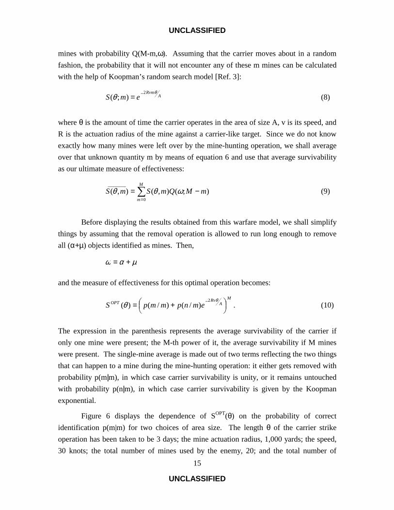
where θ is the amount of time the carrier operates in the area of size A, v is its speed, and R is the actuation radius of the mine against a carrier-like target. Since we do not know exactly how many mines were left over by the mine-hunting operation, we shall average over that unknown quantity m by means of equation 6 and use that average survivability as our ultimate measure of effectiveness:
=
−=M
mmMQmSmS
0
________
);(),(),( ωθθ (9)
Before displaying the results obtained from this warfare model, we shall simplify things by assuming that the removal operation is allowed to run long enough to remove all (α+µ) objects identified as mines. Then,
µαω +=
and the measure of effectiveness for this optimal operation becomes:
MA
RvOPT emnpmmpS
+= − θ
θ2
)/()/()( . (10)
The expression in the parenthesis represents the average survivability of the carrier if only one mine were present; the M-th power of it, the average survivability if M mines were present. The single-mine average is made out of two terms reflecting the two things that can happen to a mine during the mine-hunting operation: it either gets removed with probability p(m|m), in which case carrier survivability is unity, or it remains untouched with probability p(n|m), in which case carrier survivability is given by the Koopman exponential.
Figure 6 displays the dependence of SOPT(θ) on the probability of correct identification p(m|m) for two choices of area size. The length θ of the carrier strike operation has been taken to be 3 days; the mine actuation radius, 1,000 yards; the speed, 30 knots; the total number of mines used by the enemy, 20; and the total number of

UNCLASSIFIED
UNCLASSIFIED
16
NMBOs, 80. As can be seen from the figure, carrier survivability depends strongly on the identification probability and, as the area becomes smaller, this dependence becomes increasingly critical.
PROBABILITY OF CORRECT IDENTIFICATION
0 0.2 0.4 0.6 0.8 1.0
0.2
0.4
0.6
0.8
1.0C
ARR
IER
SU
RVI
VAB
ILIT
Y AREA SIZE
10000
2400
PROBABILITY OF CORRECT IDENTIFICATION
0 0.2 0.4 0.6 0.8 1.0
0.2
0.4
0.6
0.8
1.0C
ARR
IER
SU
RVI
VAB
ILIT
Y AREA SIZE
10000
2400
PROBABILITY OF CORRECT IDENTIFICATION
0 0.2 0.4 0.6 0.8 1.0
0.2
0.4
0.6
0.8
1.0C
ARR
IER
SU
RVI
VAB
ILIT
Y AREA SIZE
10000
2400
PROBABILITY OF CORRECT IDENTIFICATION
0 0.2 0.4 0.6 0.8 1.0
0.2
0.4
0.6
0.8
1.0C
ARR
IER
SU
RVI
VAB
ILIT
Y AREA SIZE
10000
2400
10000
2400
Figure 6. Carrier Survivability
Consequently, ascertaining the value of p(m|m) becomes an important problem. Traditionally, its value, like that of many other infrastructure parameters, is taken from Fleet empirical data. Given the purpose of our methodology, however, such procedure would not be acceptable. In fact, it is precisely this kind of habit whereby numbers are made to appear where functions should be used that is responsible for the traditional separation between structure and infrastructure issues. In what follows, we shall therefore attempt to evaluate the correct identification probability needed in the warfare model explicitly in terms of the infrastructure activities that produce it.
c. The Proficiency Model
The proficiency of the operator who performs the identification function depends on at least three factors: his natural ability for the job at hand, the quality of his original training, and the amount of experience he has gained by repeatedly executing the function since initial qualification. The first factor measures the quality of the Navy’s recruiting activity. The second factor measures the quality of the training school the operator attended upon entering the Navy. The third factor depends in turn on the operator’s seniority and the fraction of that time spent on exercising his skills. Seniority measures

UNCLASSIFIED
UNCLASSIFIED
17
the quality of all those infrastructure activities that contribute to the operator’s desire to stay in the Navy, while the fraction of time spent in exercising measures the quality of the Navy’s continuing education activities. In what follows, we shall try to describe the dependence of operator proficiency on all of these factors but will not try to extend that description to include a modeling of the infrastructure activities that underlie these factors.
To that end, let us assume that the operator emerges from training school with proficiency )( 0sϕ , where s0 measures the operator’s seniority at graduation time, and
consider the change in proficiency that occurs in the interval of time between s and (s+ds). There are clearly two ways in which proficiency can change in ds: it can increase because the operator is learning while engaged in exercising his skills, and it can decrease because the operator forgets those skills while occupied with activities unrelated to his ability to discriminate mines from NMBOs:
forgettinglearning dsdf
dsdf
dsd
−−
=
ϕϕϕ )1( (11a)
The first term represents the increase in proficiency resulting from the amount of exercising done in ds and is proportional to the probability f that the operator is currently employing his skills; the second term represents the decrease in proficiency that obtains in ds when the operator is not exercising his skills and is proportional to the probability (1-f) that the operator is currently otherwise occupied.
The two rates of change that appear in equation 11a above will, of course, depend on the specific skill under consideration, the current level at which that skill is mastered, and the specific succession of training opportunities available to the operator during his career in the Navy. Considerable research has already been done on these matters over the last century [Ref. 4] but, unfortunately, we cannot directly borrow from that research here because extant work is focused almost exclusively on improving the training process, whereas we need to focus here on the tradeoff process between structure and infrastructure instead.
Absent a model that would serve our purposes, we shall, by way of illustration, develop our own. Specifically, we shall make the simple assumption that both rates of change will be proportional to the operator’s proficiency at seniority s; this assumption merely expresses the everyday experience that people learn faster and forget faster the
UNCLASSIFIED
UNCLASSIFIED
18
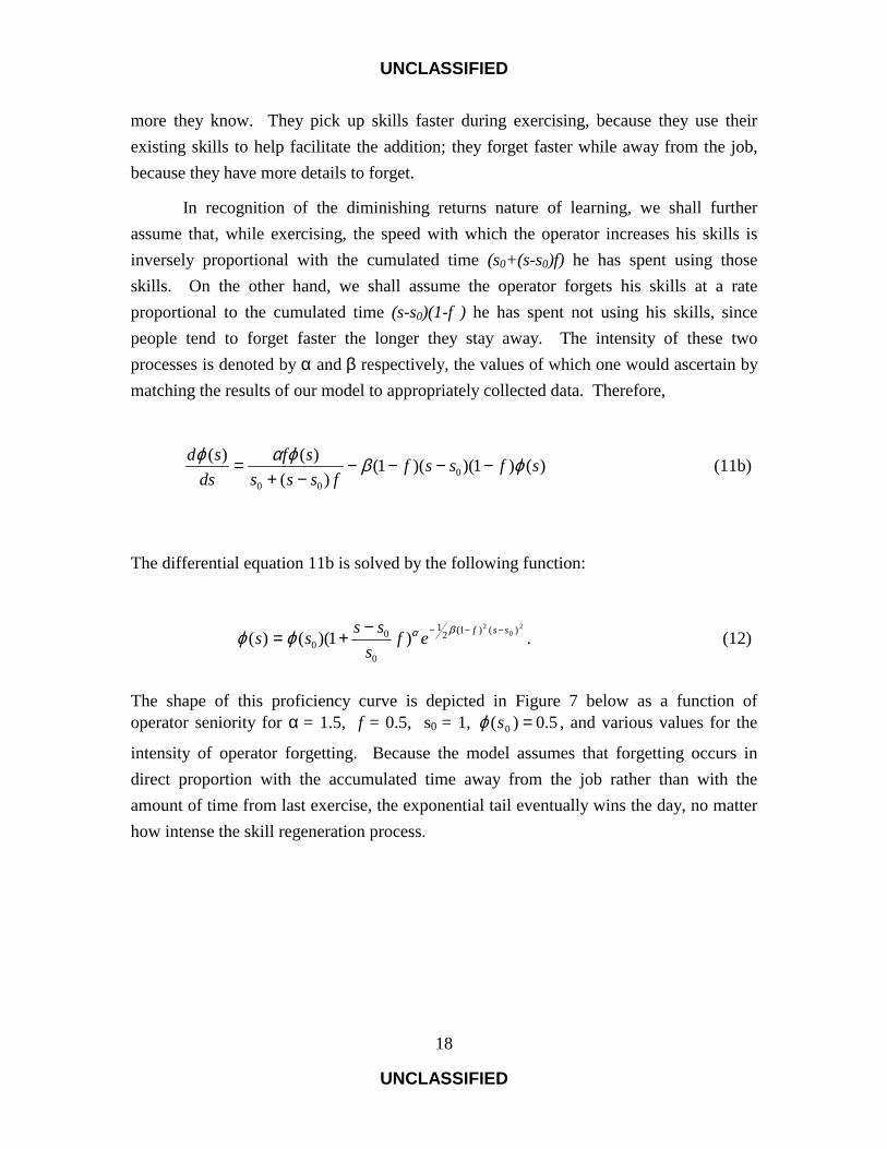
more they know. They pick up skills faster during exercising, because they use their existing skills to help facilitate the addition; they forget faster while away from the job, because they have more details to forget.
In recognition of the diminishing returns nature of learning, we shall further assume that, while exercising, the speed with which the operator increases his skills is inversely proportional with the cumulated time (s0+(s-s0)f) he has spent using those skills. On the other hand, we shall assume the operator forgets his skills at a rate proportional to the cumulated time (s-s0)(1-f ) he has spent not using his skills, since people tend to forget faster the longer they stay away. The intensity of these two processes is denoted by α and β respectively, the values of which one would ascertain by matching the results of our model to appropriately collected data. Therefore,
)()1)()(1()(
)()(0
00
sfssffsss
sfds
sd ϕβϕαϕ −−−−−+
= (11b)
The differential equation 11b is solved by the following function:
2
02 )()1(2
1
0
00 )1)(()( ssfef
sssss −−−−+= βαϕϕ . (12)
The shape of this proficiency curve is depicted in Figure 7 below as a function of operator seniority for α = 1.5, f = 0.5, s0 = 1, 5.0)( 0 =sϕ , and various values for the
intensity of operator forgetting. Because the model assumes that forgetting occurs in direct proportion with the accumulated time away from the job rather than with the amount of time from last exercise, the exponential tail eventually wins the day, no matter how intense the skill regeneration process.

UNCLASSIFIED
UNCLASSIFIED
19
OPERATOR SENIORITY (YEARS IN THE NAVY)
0 4 8 12 16 20
1.0
2.0
3.0
4.0
4.5
0.5
1.5
2.5
3.5
PRO
FIC
IEN
CY
RATE OF FORGETTING
0.05
0.10
0.25
OPERATOR SENIORITY (YEARS IN THE NAVY)
0 4 8 12 16 20
1.0
2.0
3.0
4.0
4.5
0.5
1.5
2.5
3.5
PRO
FIC
IEN
CY
RATE OF FORGETTING
0.05
0.10
0.25
Figure 7. The Proficiency Model
It is interesting to note, that if forgetting is ignored by setting β=0, the proficiency formula in equation 12 reduces to the familiar learning curve so often employed in estimating the cost of successive items in a factory production line [Ref. 5]. Indeed, if we measure production line proficiency in terms of the cost of each successive item, and identify the total time spent in exercising worker skills with the number of items produced, we get
αnCnC )0()( =
This result both verifies equation 12 with all the data supporting the learning curve and provides theoretical foundation for that largely empirical curve.
Clearly, other models based on different assumptions about the character of the instantaneous forgetting and regeneration processes are possible and, perhaps, even needed. Particularly attractive would be a model that evaluated the conditional proficiency as a function of seniority, given a particular history of exercising, and then deconditionalized that proficiency by using the marginal probability that those histories have actually materialized. However, the ability to connect infrastructure parameters, such as proficiency, to warfare capability can be demonstrated just as well with this simpler model as with a more realistic one. Since, after all, the main purpose of this

UNCLASSIFIED
UNCLASSIFIED
20
paper is to show that, and how, such connections can be made, we lose little by restricting our treatment of the problem to the simple model displayed in Figure 7. What remains important is not whether the specific form of the terms in equation 11 will survive further research but rather the fact that the proficiency process can be modeled as suggested here through a differential equation.
d. The Retention Model
In the previous section, we have derived proficiency as a function of seniority. Since we cannot control the seniority of the operators we employ in a given warfare area, it would make sense to average proficiency over the seniority distribution of operators performing the identification function. This distribution could be obtained from empirical data. However, because the data tend to be year-specific in a way that is not truly relevant to our point, we shall derive instead a simple model of that distribution, which quite closely follows typical Navy data.
Let ρ be the constant retention rate for the operator category at hand, and let us assume that each event occurs quite independently of all others. Then, the probability that there are n operators left in the Navy out of those who joined it s years ago is given by:
)/)1(,...,)2(,)1(Pr())0(Pr())(Pr( 01210,..., 110
nsnnnsn sn s
−∗∗∗∗∗ =−=====
−
νννννννν
(13)
where the summation is over all values of ν, subject to the condition that
nns −=+++ − 0121 .... ννν .
and where the “starred” symbols represent the random variables whose values are to be equal to the corresponding symbols without a star. This equation reflects the simple observation that in order to have n operators of seniority s, one must have started with n0
operators entering the Navy s years ago, an event of probability Pr(n*(0) = n0), and then lost ν1 operators the first year, ν2 the second year, and so on until the sum of all loses amounts to (n0-n). We shall now assume that the accession probability is Poisson with parameter γ and that the yearly departure process is binomial with parameter (1-ρ). One can then show that the desired probability is also Poisson, but with parameter γρs:

UNCLASSIFIED
UNCLASSIFIED
21
s
en
nsnns
γργρ −∗ ==!)())(Pr( . (14)
The probability that there are ns operators of seniority s in the Navy today is given by the fraction of operators in today’s population that have seniority s,
=
=fs
sii
ss
n
nf
0
averaged over the Poisson distribution in equation 14. If the sum in the denominator, which runs up to the maximum seniority sf, fluctuates little over the distribution in equation 14, we can take it out from under the averaging operation at its average value and have:
==
==ff s
si
i
s
s
si
i
s
sf
00
_
ρ
ρ
γρ
γρ (15)
so that the probability distribution over seniority is independent of the accession rate γ in this simple model.
It shall prove convenient to replace discrete time with a continuous variable s. Then the denominator in equation 15 becomes:
ρρρρρ
ln
0
00
sss
s
ss
i
iff
ds −= =
in which case the probability distribution over seniority s is given by:
0
ln)(____
ss
s
fsf
ρρρρ
−= (16)
This model representation of the seniority distribution, although quite simple, is not totally unrealistic. As shown in Figure 8, the model curve with 8.0=ρ fits rather
well the 1998 and 1999 data [Ref. 6] for sonar operators in the midrange, overestimates for low seniority, and underestimates somewhat for high seniority. This latter is

UNCLASSIFIED
UNCLASSIFIED
22
undoubtedly the result of the natural tendency enlisted personnel have of staying in for the 20-year retirement package, a fact clearly not included in our model.
OPERATOR SENIORITY IN YEARS
0 5 10 15 20
PRO
BAB
ILIT
Y
0.05
0.10
0.15
0.20
0.25
0.30
1998 Data
1999 Data
Model
OPERATOR SENIORITY IN YEARS
0 5 10 15 20
PRO
BAB
ILIT
Y
0.05
0.10
0.15
0.20
0.25
0.30
1998 Data
1999 Data
Model
Figure 8. The Retention Model
Combining the proficiency model at equation 12 with the retention model at equation 16, we can finally write down the average operator proficiency as:
20
2
00
)()1(21
0
00
_)1(
)(ln)( ssf
s
sss
s
efs
ssdss
f
f
−−−−+
−=
βα
ρρρρϕϕ (17)
e. Connecting Infrastructure to Warfare
We are now ready to deliver on the promise made at the beginning of this section and display the explicit connection between infrastructure parameters, such as proficiency at time of graduation, learning and forgetting rates, retention rate, and fraction of the year that operators are engaged in using their skills, on the one hand, with the measure of operational effectiveness described by carrier survivability on the other. To do so, we need only identify the proficiency ϕ with the probability of correct
UNCLASSIFIED
UNCLASSIFIED
23
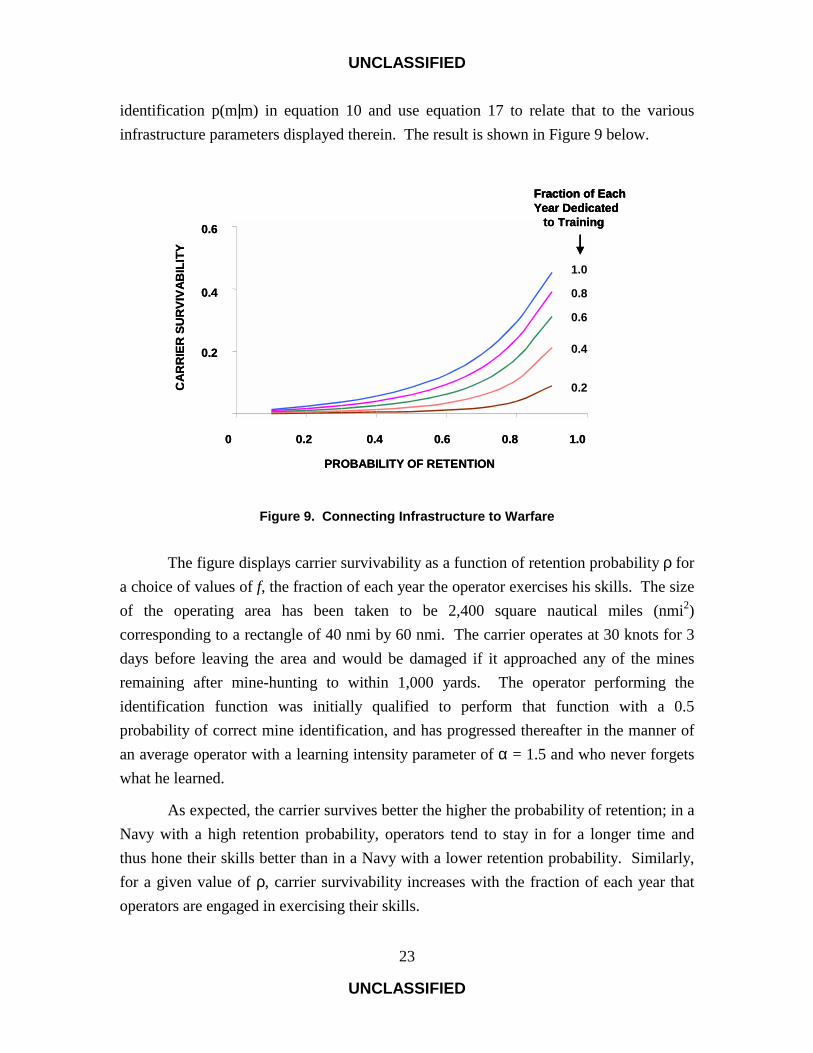
identification p(m|m) in equation 10 and use equation 17 to relate that to the various infrastructure parameters displayed therein. The result is shown in Figure 9 below.
0 0.2 0.4 0.6 0.8 1.0
0.2
0.4
0.6
PROBABILITY OF RETENTION
CAR
RIE
R S
UR
VIVA
BIL
ITY
Fraction of EachYear Dedicated
to Training
0.2
0.4
0.6
0.8
1.0
0 0.2 0.4 0.6 0.8 1.0
0.2
0.4
0.6
PROBABILITY OF RETENTION
CAR
RIE
R S
UR
VIVA
BIL
ITY
Fraction of EachYear Dedicated
to Training
Fraction of EachYear Dedicated
to Training
0.2
0.4
0.6
0.8
1.0
Figure 9. Connecting Infrastructure to Warfare
The figure displays carrier survivability as a function of retention probability ρ for a choice of values of f, the fraction of each year the operator exercises his skills. The size of the operating area has been taken to be 2,400 square nautical miles (nmi2) corresponding to a rectangle of 40 nmi by 60 nmi. The carrier operates at 30 knots for 3 days before leaving the area and would be damaged if it approached any of the mines remaining after mine-hunting to within 1,000 yards. The operator performing the identification function was initially qualified to perform that function with a 0.5 probability of correct mine identification, and has progressed thereafter in the manner of an average operator with a learning intensity parameter of α = 1.5 and who never forgets what he learned.
As expected, the carrier survives better the higher the probability of retention; in a Navy with a high retention probability, operators tend to stay in for a longer time and thus hone their skills better than in a Navy with a lower retention probability. Similarly, for a given value of ρ, carrier survivability increases with the fraction of each year that operators are engaged in exercising their skills.
UNCLASSIFIED
UNCLASSIFIED
24
The infrastructure parameters that determine carrier survivability depend in turn on the infrastructure activities that produce operators with those characteristics. Thus, a Navy with an extensive quality of life program will exhibit a high retention probability; and similarly, a Navy that takes the time to frequently provide realistic training will produce a large value of f. Both of these activities will directly contribute to a higher carrier survivability, as will the maintenance of a high-quality training school able to produce students who will start their careers with a high probability of correct mine identification p(m|m). Unfortunately, since our illustrative model does not capture the structure of these activities, it cannot shed any light on their relative cost-effectiveness and will therefore not allow us to consider tradeoffs between them. The next illustrative example, however, will.
2. Area Clearance ASW Operations
a. Operational Setting
The organic MCM example considered in Section C.1 showed us that the methodology championed here can be meaningfully implemented. The second example will show that, once implemented, it could also help decision makers trade between equal cost structure and infrastructure investments by illuminating their relative contribution to warfare capability. This second example will therefore start with a real decision issue the Navy faces today.
The decision concerns the desirability of building a shallow-water ASW training facility on each coast for the purpose of improving the Fleet’s ability to perform littoral operations. Some believe that building such facilities would significantly increase warfare capability and would do so without undue expenditure of funds. Others believe that the same benefits can be had by acquiring a few more ASW platforms to provide for increased realistic training opportunities. Underlying this debate is the assumption that what ails our littoral ASW capability is not equipment performance but operator proficiency. Since no quantitative modeling is available to connect proficiency to warfare capability, the debate is waged at a subjective level, and victory would go to those who carry the political power, not necessarily to those who are right.
In what follows, we show that our methodology could bring light to this debate. To that end, we choose to embed the decision issue into a typical ASW problem, that of providing precursor area clearance to carrier strike operations. This operation is

UNCLASSIFIED
UNCLASSIFIED
25
performed by surface ships sweeping the prospective operating area for enemy submarines that may be lying in wait for the carrier battle group and is depicted in Figure 10 below.
AREA OF CARRIER
OPERATION
Median Detection Range
AREA OF CARRIEROPERATION
Median Detection Range
Figure 10. Generic Precursor Area Clearance Operation
As shown in the figure, a number of ASW surface ships, each with its characteristic median detection range, search the operating area. By the definition of the median detection range W, any enemy submarine that enters the circle of radius W surrounding an ASW ship is detected with certainty, but any submarine outside this circle remains undetected. As the surface ship moves back and forth, the circle of radius W sweeps out the section of operating area that has been assigned to it and thus, in due time, the ASW force sweeps out the entire operating area. Any submarine that has been detected is then subjected to repeated attacks until the ship succeeds in sinking the submarine or the submarine escapes the encounter alive.
After the operation is allowed to proceed for a time τ, the ASW force withdraws, and the carrier battle group moves in to begin performing its strike mission with the hope that it will not have to worry any longer about enemy submarines. In reality, of course, no ASW operation ever succeeds completely, and some of the submarines may remain in the area ready to attack the aircraft carriers. Since the battle group commander would like to minimize the chance of this happening, a natural measure of effectiveness for the precursor operation is the probability that the carrier will not be attacked by submarines during the execution of its mission.

UNCLASSIFIED
UNCLASSIFIED
26
b. The Warfare Model
This measure of effectiveness can be evaluated by creating a quantitative model of the activities described above. The simplest such model is provided by Koopman’s random search model. Assuming that only one enemy submarine was in the area to begin with and that no others enter the area after the clearance operation has been completed, the Koopman model provides the following expression for the probability that the one enemy submarine will be killed during a precursor operation lasting τ days:
ANWvpk
eWPτ2
1)( −−= (18)
where A is the area of the carrier operating box, v is the speed of the ASW ship relative to that of the enemy submarine, N is the number of such ships, W is the median detection range of the sonar employed aboard ship, and pk is the probability that the ship will kill the submarine given that it has detected it. The median detection range W, in turn, is strongly affected by the sonarman’s ability to tell signal from noise
40)(
10)(RDDIANSL
RDW−+−
= . (19)
where the recognition differential RD is defined as the smallest amount of signal the operator can pick out of the surrounding noise.
This latter equation, called the sonar equation [Ref. 7], describes the performance of a noise-limited, active sonar as a function of the target’s source level SL, the prevailing ambient noise AN, the array directivity index DI, and the operator recognition differential RD, if the sound propagation through the water is described by a spherical spreading law. Given the very short detection ranges typical of modern sonar against quiet diesel submarines, this assumption should be quite accurate.
In practice, standard values for RD are inserted in the sonar equation, values whose provenance is uniformly obscure. By contrast, because it is operator proficiency that really interests us here, we have been careful to explicitly display the dependence on recognition differential and refrained from replacing it by numerical values. Instead, we shall use the proficiency model developed in the previous section. Specifically, we take the proficiency ϕ to be the recognition differential; equation 17 will then provide the
recognition differential as a function of the retention rate ρ, the learning rate α, the forgetting rate β, and the training frequency f:

UNCLASSIFIED
UNCLASSIFIED
27
20
2
00
)()1(21
0
00
___
)1()(
ln)( ssfs
sss
s
efs
ssdssRDRD
f
f
−−−−+
−=
βα
ρρρρ (20)
Replacing equation 20 into equation 19, we obtain the desired connection between ASW capability and infrastructure parameters displayed in Figure 11.
NUMBER OF SHIP-DAYS DEDICATED TO ASW
0 1 2 3 4 5 6
0.2
0.4
0.6
0.8
1.0
CAR
RIE
R S
UR
VIVA
BIL
ITY
FRACTION OF YEARDEDICATED TO ASW
TRAINING
0.2
0.8
NUMBER OF SHIP-DAYS DEDICATED TO ASW
0 1 2 3 4 5 6
0.2
0.4
0.6
0.8
1.0
0.2
0.4
0.6
0.8
1.0
CAR
RIE
R S
UR
VIVA
BIL
ITY
FRACTION OF YEARDEDICATED TO ASW
TRAINING
0.2
0.8
Figure 11. Effectiveness of Precursor ASW Operations
As shown in the figure, carrier survivability is a function of both the number Nτ of ship-days that constitutes the ASW effort dedicated to the precursor operation, and on the amount of training provided to the sonar operator. This fact, however, is not of primary importance for us at this point in the argument; after all, the possibility of connecting warfare to the infrastructure activities that contribute to the production of whatever structure elements are employed in the execution of the mission under consideration has already been demonstrated in the previous section. What is of importance here is to demonstrate the ability of our methodology to aid the decision maker in the performance of his task. How that’s done is the subject of the next section.

UNCLASSIFIED
UNCLASSIFIED
28
c. The Tradeoff Analysis
As already mentioned, the decision to be made concerns the desirability of investing in training for shallow-water ASW as against investing in increasing the ASW effort. It is apparent that the effectiveness model described above is well suited for dealing with this question. Indeed, all we must to do is display the results in Figure 11, not in terms of carrier survivability as a function of Nτ and f, but in terms of equi-effectiveness curves in the universe spanned by those two parameters.
PROBABILITY THAT CARRIER
IS NOT ATTACKED
FRACTION OF THE YEAR OPERATOR GETS REALISTIC TRAINING
0 0.1 0.2 0.3 0.4 0.5
1
23
4
5
6
0.10.20.30.40.5
0.6
0.7
SHIP
-DA
YS
DED
ICA
TED
TO
ASW
PROBABILITY THAT CARRIER IS NOT ATTACKED
FRACTION OF THE YEAR OPERATOR GETS REALISTIC TRAINING
0 0.1 0.2 0.3 0.4 0.5
1
23
4
5
6
1
23
4
5
6
0.10.20.30.40.5
0.6
0.7
SHIP
-DA
YS
DED
ICA
TED
TO
ASW
Figure 12. The Tradeoff Space
The result is displayed in Figure 12 above. All combinations of Nτ and f that trace out a given curve in this space produce the same probability that the carrier is not attacked. The star might represent a reasonable assessment of the current situation; its location in the plane indicates that, for the situation described here, current survivability probably amounts to no more than 0.3, fully justifying the Navy‘s concern with shallow-water ASW capability that we hypothesized here.
There are at least two different ways of improving this capability: either increase f or increase Nτ. The first option corresponds to the development of the shallow-water ASW training centers mentioned at the beginning of this section. The second option represents the position taken by those that oppose the building of these facilities. The

UNCLASSIFIED
UNCLASSIFIED
29
cost associated with the first option is approximately $100 million per facility. With that kind of money, the Navy could not buy new ships and would, therefore, have to increase Nτ by buying additional ship-time from the existing pool of ASW ships. This latter, however, is a relatively cheap commodity, and one could buy a lot of it with the price of one training facility. The situation is depicted in Figure 13, which displays the two options discussed here.
AVERAGE PROBABILITY THAT CARRIER IS NOT ATTACKED
FRACTION OF THE YEAR OPERATOR GETS REALISTIC TRAINING
0 0.1 0.2 0.3 0.4 0.5
1
23
4
5
6
0.10.20.30.40.5
0.6
0.7
SHIP
-DAY
S D
EDIC
ATED
TO
ASW
Shallow Water ASWTraining Range
Investment
AVERAGE PROBABILITY THAT CARRIER IS NOT ATTACKED
FRACTION OF THE YEAR OPERATOR GETS REALISTIC TRAINING
0 0.1 0.2 0.3 0.4 0.5
1
23
4
5
6
0.10.20.30.40.5
0.6
0.7
SHIP
-DAY
S D
EDIC
ATED
TO
ASW
Shallow Water ASWTraining Range
Investment
Figure 13. Investment Options
We do not really know that building shallow-water training centers would increase f from 0.05 to 0.25 as indicated in the figure, but given the disparity in the cost of the two options, that is hardly important. What maters is the fact, apparent in the figure, that investing in the training center is bound to improve ASW effectiveness over the current value more than the same investment in buying operating time. The reason for this is that the equi-effectiveness curves bunch up around the location of the current capability point indicated by the star, and extending the vertical arrow upward tends to produce little, if any, change in ASW effectiveness regardless of how far we extend the arrow. On the other hand, extending the horizontal arrow rightward far beyond the f = 0.25 point would similarly produce very little change in effectiveness. Therefore, the

UNCLASSIFIED
UNCLASSIFIED
30
next dollar should be invested in ASW training, at least until the fraction of time spent in realistic training reaches 0.25; afterwards, the Navy should invest its ASW money in buying sufficient ASW effort to increase the amount it can dedicate to this mission.
One could argue that increasing each year the fraction dedicated to training does not necessarily require the building of these facilities. Instead, one may simply have sailors spend more time in exercises or in front of computer simulators. However, exercises are expensive and, therefore, hard to come by, while trainers are only simulations, not the real thing; getting an instrumented range such as that available in a training center appears to be the right way to go.
D. THE WAY AHEAD
We have reached the end of our argument. Along the way, we have developed a methodology able to quantitatively connect the quality of infrastructure activities to the Navy’s warfare capability. The major advantage of this methodology is that it would help the Navy trade infrastructure investments for investments in naval structure without having to worry about the possibility that warfare capability would thereby be lost. The disadvantage is that it requires a lot more work, analytic and experimental, than the subjective alternatives employed today.
Lest the disadvantages strangle the methodology, let us hasten to remember that no analytic methodology has ever come fast and cheap. The development of warfare models in which infrastructure is ignored has itself been long in coming; in fact, their development has taken most of the last half of the 20th century and has cost a considerable amount of money. Surely, if the Navy has been patient and generous enough to reach the sophistication evident in our current warfare modeling, it cannot fail to demonstrate the same qualities now that the shortage of funds has made it necessary to develop new tools to handle the infrastructure problem.
There is much to be done in achieving that goal, but there seems to be light at the end of the tunnel. The preliminary proficiency model developed in this paper stands as a beacon showing the way. While important, this is not enough. There are at least two more analytic hurdles to overcome. One would be to try and extend the sailor proficiency model described here into a model designed to capture the behavior of well-organized groups of sailors forming the crews of a naval platform. There is good reason to believe that the behavior of such crews is significantly different from the simple sum of their

UNCLASSIFIED
UNCLASSIFIED
31
components, much like the defensive capability of a carrier is more robust than the simple sum of its defensive layers.
The second hurdle is the need to explicitly model infrastructure activities with the goal of evaluating the change in the quality of the people and objects produced corresponding to a given investment in that activity. Until now, infrastructure models were used to help manage the activities involved, not to measure the quality of their output in a manner fit for use in warfare modeling. On this point, our paper has not helped much beyond describing how one would connect such models, if one had them, to trading investments. We would hope, however, that the opportunity to do so will present itself soon.
Until then, it would be useful to improve upon the models presented here. As a minimum, one would want to explore the possibility of adding real histories to the proficiency model and, perhaps, explore various other, more realistic, ways of representing the learning and forgetting processes. Similarly, one might want to incorporate a quantitative model of the operator proficiency at graduation. Generally, schools generate graduates with a Gaussian distribution of skills. All one needs to do is to translate the relative grades employed today with an absolute scale related to the parameter that best measures the student’s ability to perform the job to which he is going. For instance, instead of the grades operators receive upon graduation from the school training them to tell mines from NMBOs, one might want to measure the number of false alarms each graduate produces when confronted with the standard operational set of circumstances he will encounter on the job.

UNCLASSIFIED
UNCLASSIFIED
32
REFERENCES
1. Philip M. Morse & Herman Feshbach, Methods of Theoretical Physics, McGraw-Hill, 1953.
2. William Feller, An Introduction to Probability Theory and Its Applications, John Wiley & Sons, Inc., 1968.
3. B. O. Koopman, Search and Screening, Operational Evaluation Group, 1946.
4. Mark A. Sabol & Robert A. Wisher, “Retention and Reacquisition of Military Skills,” Military Operations Research, Vol. 6, Nr. 1, 2001.
5. J. W. Noah & R. W. Smith, “Cost-Quantity Calculator,” The RAND Corporation, Memorandum RM-2786-PR, 1962.
6. Defense Manpower Data Center (www.dmdc.osd.mil/).
7. Robert J. Urick, Principles of Underwater Sound, McGraw-Hill, 1967.

UNCLASSIFIED
UNCLASSIFIED
Appendix A DISTRIBUTION LIST FOR IDA PAPER P-3605


UNCLASSIFIED
UNCLASSIFIED
A-1
Appendix A DISTRIBUTION LIST FOR IDA PAPER P-3605
Department of Defense No. of copies Office of the Secretary of Defense Under Secretary of Defense (Personnel and Readiness) Pentagon, Room 3E764 Washington, DC. 20301 1 Office of the Secretary of Defense Acquisition, Technology & Logistics Naval Warfare Division Pentagon, Room 3D1048 Washington, DC. 20301 Attn: Dr. Paris Genalis 1 Mr. George Leineweber 1 Office of the Secretary of Defense Assistant Secretary of Defense (Force Management Policy) Pentagon, Room 3E784 Washington, DC. 20301 1 Office of the Secretary of Defense Director (Program Analysis & Evaluation) Pentagon, Room 3E836 Washington, DC. 20301 1 Joint Chiefs of Staff Director of Manpower Personnel (J-1) Pentagon, Room 1E948 Washington, DC. 20318 1

UNCLASSIFIED
UNCLASSIFIED
A-2
Joint Chiefs of Staff (Cont.) No. of copies Director for Force Structure, Resources And Assessment (J-8) Pentagon Washington, DC. 20318 1 Department of the Navy Under Secretary of the Navy, Pentagon, Room 4E732 Washington, DC. 20350 1 Assistant Secretary of the Navy (Manpower & Reserve Affairs), Pentagon, Room 4E788 Washington, DC. 20350 1 Deputy Assistant Secretary of the Navy (Manpower) Pentagon, Room 4E789 Washington, DC. 20350 Attn: Mrs. Bonnie Morehouse 1 Assistant Secretary of the Navy (Research, Development & Acquisition) Pentagon, Room 4E741 Washington, DC. 20350 1 Deputy Assistant Secretary of the Navy (Mine/Undersea Warfare) Pentagon, Room 5C738 Washington, DC. 20350 1 Deputy Chief of Naval Operations (Manpower & Personnel) N1 Pentagon, Room 2072 Washington, DC. 20350 1 Deputy Chief of Naval Operations (Manpower & Personnel) Director Total Force Programming Manpower & IRM Division, N12 Pentagon, Room 2827 Washington, DC. 20350 1

UNCLASSIFIED
UNCLASSIFIED
A-3
Department of the Navy (Cont.) No. of copies Deputy Chief of Naval Operations (Naval Warfare) N7 Pentagon, Room 4E536 Washington, DC. 20350 1 Manpower Training Requirements Branch, N759 Pentagon, Room 4A720 Washington, DC. 20350 1 Deputy Chief of Naval Operations (Naval Warfare), Director Naval Education and Training, N79 Pentagon, Room 4E542 Washington, DC. 20350 1 Deputy Chief of Naval Operations Surface Warfare Division, N76 Pentagon, Room 4E552 Washington, DC. 20350 1 Deputy Chief of Naval Operations (Resources, Warfare Requirements, Assessments, N8 Pentagon, Room 4E620 Washington, DC. 20350 1 Deputy Chief of Naval Operations (Resources, Warfare Requirements, Assessments), Assessment Division N81 Pentagon, Room 4A531 Washington, DC. 20350 1 Attn: CDR Matt Peters, Room 4A4307 1 Department of the Air Force Assistant Secretary (Manpower, Reserve Affairs, Installations & Environment) SAF/MI Pentagon, Room 4E1020 Washington, DC. 20330 1 Deputy Chief of Staff Personnel Pentagon, Room 4E194 Washington, DC. 20330 1

UNCLASSIFIED
UNCLASSIFIED
A-4
Department of the Air Force (Cont.) No. of copies Deputy Chief of Staff (Plans & Programs) AF/XP Pentagon, Room 5E124 Washington, DC. 20330 1 Department of the Army Assistant Secretary of the Army (Manpower & Reserve Affairs) Pentagon, Room 2E594 Washington, DC. 20310 1 Deputy Chief of Staff for Personnel Pentagon, Room 2E736 Washington, DC. 20310 1 Deputy Chief of Staff Operation & Plans (DAMO-ZA) Pentagon, Room 3E636 Washington, DC. 20310 1 Other Organizations Defense Technical Information Center 8725 John H. Kingman Road STE 0944 Fort Belvoir, VA 22060-6218 2 Institute for Defense Analyses 1801 North Beauregard Street Alexandria, VA 22311-1772 15 Total Distribution 44

REPORT DOCUMENTATION PAGE Form Approved OMB No. 0704-0188
Public reporting burden for this collection of information is estimated to average 1 hour per response, including the time for reviewing instructions, searching existing data sources, gathering and maintaining the data needed, and completing and reviewing the collection of information. Send comments regarding this burden estimate or any other aspect of this collection of information, including suggestions for reducing this burden, to Washington Headquarters Services, Directorate for Information Operations and Reports, 1215 Jefferson Davis Highway, suite 1204, Arlington, VA 22202-4302, and to the Office of Management and Budget, Paperwork Reduction Project (0704-0188), Washington, DC 20503. 1. AGENCY USE ONLY (Leave blank)
2. REPORT DATE
March 2001 3. REPORT TYPE AND DATES COVERED
Final 4. TITLE AND SUBTITLE
Gauging the Military Value of Naval Infrastructure
5. FUNDING NUMBERS
DASW-01-98-C-0067
6. AUTHOR(S)
Alfred I. Kaufman, Edward Zdnakiewicz
Task No. AB-1-1680
7. PERFORMING ORGANIZATION NAME(S) AND ADDRESS(ES)
Institute for Defense Analyses 1801 N. Beauregard Street Alexandria, VA 22311-1772
8. PERFORMING ORGANIZATION REPORT NUMBER
IDA Paper P-3605
9. SPONSORING/MONITORING AGENCY NAME(S) AND ADDRESS(ES)
Office of the Under Secretary of Defense FFRDC Programs (Acquisition, Technology, and Logistics) 2001 N. Beauregrad Street Naval Warfare Division, Alexandria, VA 22311-1772 Pentagon, Room 3D 1048 Washington, DC 20301 Attn: Mr. George Leineweber Assessment Division, Office of the Deputy Chief of Naval Operations (Resources, Warfare Requirements, and Assessments) The Naval Annex, Room 4319 Arlington, VA 22202 Attn: Mr. Richard Robins (N813)
10. SPONSORING/MONITORING AGENCY REPORT NUMBER
11. SUPPLEMENTARY NOTES
12a. DISTRIBUTION/AVAILABILITY STATEMENT
Approved for public release; distribution unlimited.
12b. DISTRIBUTION CODE
13. ABSTRACT (Maximum 200 words)
This paper proposes a methodology for relating investments in naval infrastructure programs to investment programs in naval structure and illustrates the utility of such a methodology in trading infrastructure for structure by applying the methodology to organic mine countermeasure and shallow water antisubmarine operations.
15. NUMBER OF PAGES
45 14. SUBJECT TERMS
naval infrastructure; naval structure; human proficiency; recruitment; retention; training; mine countermeasures; shallow-water antisubmarine warfare
16. PRICE CODE
17. SECURITY CLASSIFICATION OF REPORT
UNCLASSIFIED
18. SECURITY CLASSIFICATION OF THIS PAGE
UNCLASSIFIED
19. SECURITY CLASSIFICATION OF ABSTRACT
UNCLASSIFIED
20. LIMIT OF ABSTRACT
Unlimited
NSN7540-01-280-5500 Standard Form 298 (Rev. 2-89) Prescribed by ANSI Std. Z39-18 298-102