Embed Size (px)
Citation preview

Coning is a term used to describe the mechanism underlying theupward movement of water and/or the down movement of gas into theperforations of a producing well. Coning can seriously impact the wellproductivity and influence the degree of depletion and the overall recov-ery efficiency of the oil reservoirs. The specific problems of water andgas coning are listed below.
• Costly added water and gas handling• Gas production from the original or secondary gas cap reduces pressure
without obtaining the displacement effects associated with gas drive• Reduced efficiency of the depletion mechanism• The water is often corrosive and its disposal costly• The afflicted well may be abandoned early• Loss of the total field overall recovery
Delaying the encroachment and production of gas and water are essen-tially the controlling factors in maximizing the field’s ultimate oil recov-ery. Since coning can have an important influence on operations, recov-ery, and economics, it is the objective of this chapter to provide thetheoretical analysis of coning and outline many of the practical solutionsfor calculating water and gas coning behavior.
583
C H A P T E R 9
GAS AND WATER CONING
© 2010 Elsevier Inc. All rights reserved.Doi: 10.1016/C2009-0-30429-8
CONING
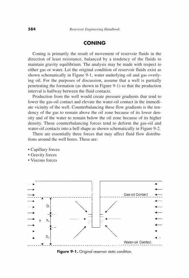
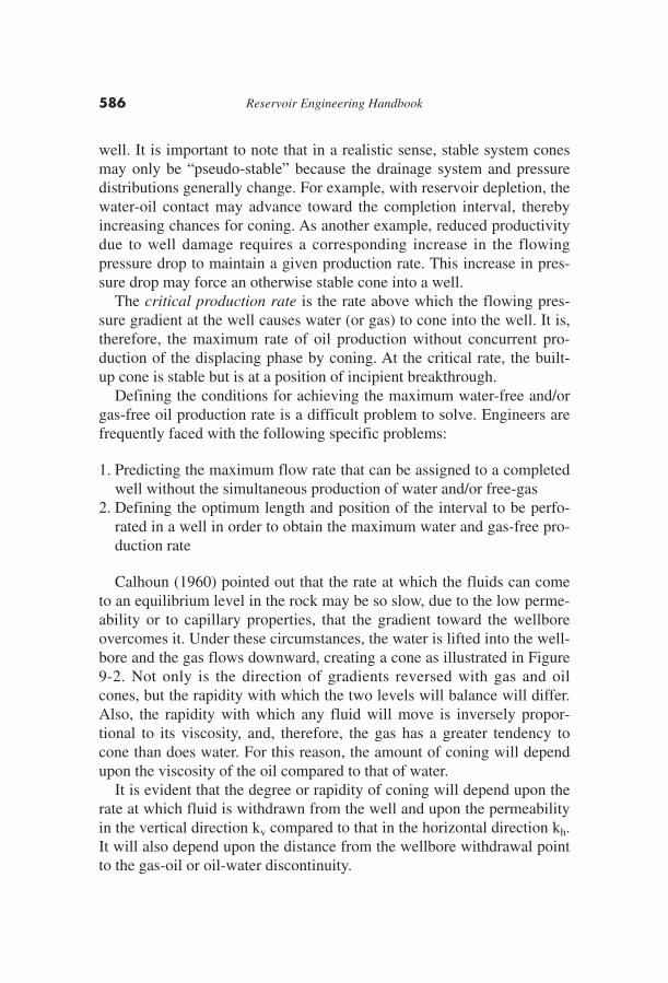
Coning is primarily the result of movement of reservoir fluids in thedirection of least resistance, balanced by a tendency of the fluids tomaintain gravity equilibrium. The analysis may be made with respect toeither gas or water. Let the original condition of reservoir fluids exist asshown schematically in Figure 9-1, water underlying oil and gas overly-ing oil. For the purposes of discussion, assume that a well is partiallypenetrating the formation (as shown in Figure 9-1) so that the productioninterval is halfway between the fluid contacts.
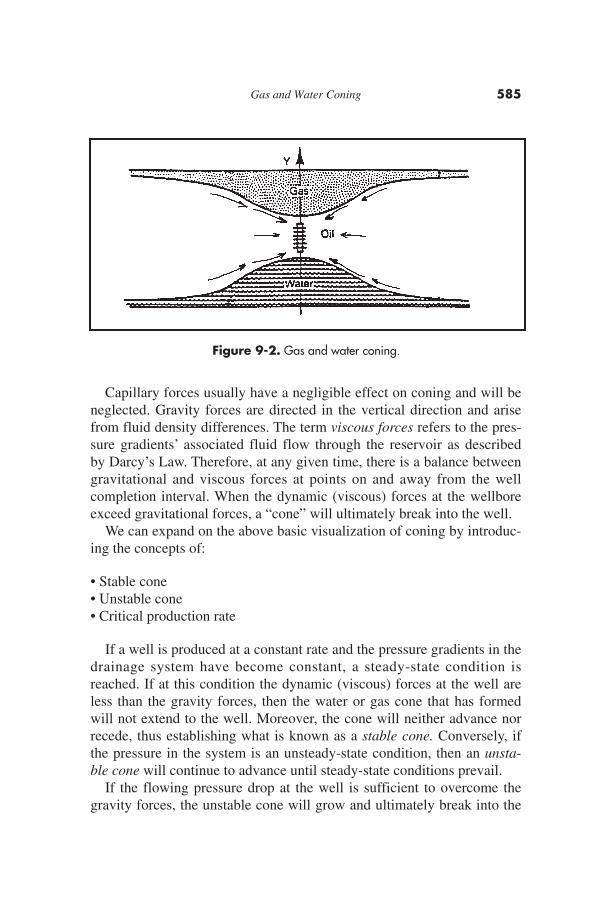
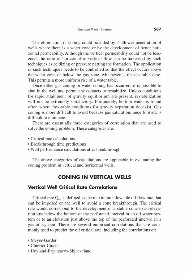
Production from the well would create pressure gradients that tend tolower the gas-oil contact and elevate the water-oil contact in the immedi-ate vicinity of the well. Counterbalancing these flow gradients is the ten-dency of the gas to remain above the oil zone because of its lower den-sity and of the water to remain below the oil zone because of its higherdensity. These counterbalancing forces tend to deform the gas-oil andwater-oil contacts into a bell shape as shown schematically in Figure 9-2.
There are essentially three forces that may affect fluid flow distribu-tions around the well bores. These are:
• Capillary forces• Gravity forces• Viscous forces
584 Reservoir Engineering Handbook
Figure 9-1. Original reservoir static condition.
Capillary forces usually have a negligible effect on coning and will beneglected. Gravity forces are directed in the vertical direction and arisefrom fluid density differences. The term viscous forces refers to the pres-sure gradients’ associated fluid flow through the reservoir as describedby Darcy’s Law. Therefore, at any given time, there is a balance betweengravitational and viscous forces at points on and away from the wellcompletion interval. When the dynamic (viscous) forces at the wellboreexceed gravitational forces, a “cone” will ultimately break into the well.
We can expand on the above basic visualization of coning by introduc-ing the concepts of:
• Stable cone• Unstable cone• Critical production rate
If a well is produced at a constant rate and the pressure gradients in thedrainage system have become constant, a steady-state condition isreached. If at this condition the dynamic (viscous) forces at the well areless than the gravity forces, then the water or gas cone that has formedwill not extend to the well. Moreover, the cone will neither advance norrecede, thus establishing what is known as a stable cone. Conversely, ifthe pressure in the system is an unsteady-state condition, then an unsta-ble cone will continue to advance until steady-state conditions prevail.
If the flowing pressure drop at the well is sufficient to overcome thegravity forces, the unstable cone will grow and ultimately break into the
Gas and Water Coning 585
Figure 9-2. Gas and water coning.
well. It is important to note that in a realistic sense, stable system conesmay only be “pseudo-stable” because the drainage system and pressuredistributions generally change. For example, with reservoir depletion, thewater-oil contact may advance toward the completion interval, therebyincreasing chances for coning. As another example, reduced productivitydue to well damage requires a corresponding increase in the flowingpressure drop to maintain a given production rate. This increase in pres-sure drop may force an otherwise stable cone into a well.
The critical production rate is the rate above which the flowing pres-sure gradient at the well causes water (or gas) to cone into the well. It is,therefore, the maximum rate of oil production without concurrent pro-duction of the displacing phase by coning. At the critical rate, the built-up cone is stable but is at a position of incipient breakthrough.
Defining the conditions for achieving the maximum water-free and/orgas-free oil production rate is a difficult problem to solve. Engineers arefrequently faced with the following specific problems:
1. Predicting the maximum flow rate that can be assigned to a completedwell without the simultaneous production of water and/or free-gas
2. Defining the optimum length and position of the interval to be perfo-rated in a well in order to obtain the maximum water and gas-free pro-duction rate
Calhoun (1960) pointed out that the rate at which the fluids can cometo an equilibrium level in the rock may be so slow, due to the low perme-ability or to capillary properties, that the gradient toward the wellboreovercomes it. Under these circumstances, the water is lifted into the well-bore and the gas flows downward, creating a cone as illustrated in Figure9-2. Not only is the direction of gradients reversed with gas and oilcones, but the rapidity with which the two levels will balance will differ.Also, the rapidity with which any fluid will move is inversely propor-tional to its viscosity, and, therefore, the gas has a greater tendency tocone than does water. For this reason, the amount of coning will dependupon the viscosity of the oil compared to that of water.
It is evident that the degree or rapidity of coning will depend upon therate at which fluid is withdrawn from the well and upon the permeabilityin the vertical direction kv compared to that in the horizontal direction kh.It will also depend upon the distance from the wellbore withdrawal pointto the gas-oil or oil-water discontinuity.
586 Reservoir Engineering Handbook
The elimination of coning could be aided by shallower penetration ofwells where there is a water zone or by the development of better hori-zontal permeability. Although the vertical permeability could not be less-ened, the ratio of horizontal to vertical flow can be increased by suchtechniques as acidizing or pressure parting the formation. The applicationof such techniques needs to be controlled so that the effect occurs abovethe water zone or below the gas zone, whichever is the desirable case.This permits a more uniform rise of a water table.
Once either gas coning or water coning has occurred, it is possible toshut in the well and permit the contacts to restabilize. Unless conditionsfor rapid attainment of gravity equilibrium are present, restabilizationwill not be extremely satisfactory. Fortunately, bottom water is foundoften where favorable conditions for gravity separation do exist. Gasconing is more difficult to avoid because gas saturation, once formed, isdifficult to eliminate.
There are essentially three categories of correlation that are used tosolve the coning problem. These categories are:
• Critical rate calculations• Breakthrough time predictions• Well performance calculations after breakthrough
The above categories of calculations are applicable in evaluating theconing problem in vertical and horizontal wells.
CONING IN VERTICAL WELLS
Vertical Well Critical Rate Correlations
Critical rate Qoc is defined as the maximum allowable oil flow rate thatcan be imposed on the well to avoid a cone breakthrough. The criticalrate would correspond to the development of a stable cone to an eleva-tion just below the bottom of the perforated interval in an oil-water sys-tem or to an elevation just above the top of the perforated interval in agas-oil system. There are several empirical correlations that are com-monly used to predict the oil critical rate, including the correlations of:
• Meyer-Garder• Chierici-Ciucci• Hoyland-Papatzacos-Skjaeveland
Gas and Water Coning 587
• Chaney et al.• Chaperson• Schols
The practical applications of these correlations in predicting the criti-cal oil flow rate are presented over the following pages.
The Meyer-Garder Correlation
Meyer and Garder (1954) suggest that coning development is a resultof the radial flow of the oil and associated pressure sink around the well-bore. In their derivations, Meyer and Garder assume a homogeneous sys-tem with a uniform permeability throughout the reservoir, i.e., kh = kv . Itshould be pointed out that the ratio kh/kv is the most critical term in eval-uating and solving the coning problem. They developed three separatecorrelations for determining the critical oil flow rate:
• Gas coning• Water coning• Combined gas and water coning
Gas coning
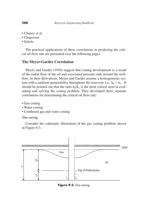
Consider the schematic illustration of the gas coning problem shownin Figure 9-3.
588 Reservoir Engineering Handbook
Figure 9-3. Gas coning.
Meyer and Garder correlated the critical oil rate required to achieve astable gas cone with the following well penetration and fluid parameters:
• Difference in the oil and gas density• Depth Dt from the original gas-oil contact to the top of the perforations• The oil column thickness h
The well perforated interval hp, in a gas-oil system, is essentiallydefined as
hp = h − Dt
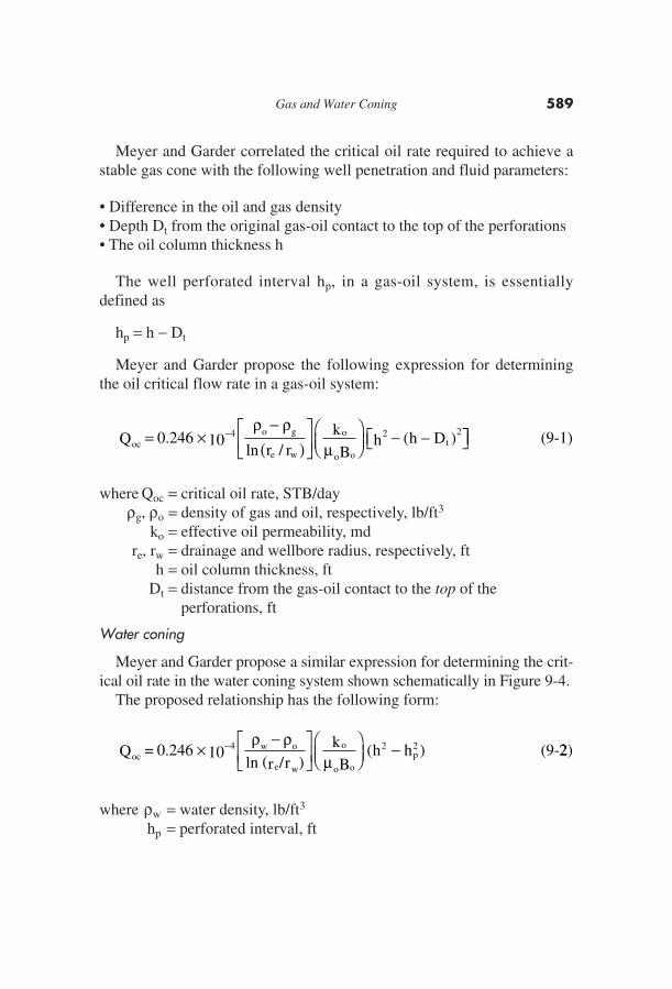
Meyer and Garder propose the following expression for determiningthe oil critical flow rate in a gas-oil system:
where Qoc = critical oil rate, STB/dayρg, ρo = density of gas and oil, respectively, lb/ft3
ko = effective oil permeability, mdre, rw = drainage and wellbore radius, respectively, ft
h = oil column thickness, ftDt = distance from the gas-oil contact to the top of the
perforations, ft
Water coning
Meyer and Garder propose a similar expression for determining the crit-ical oil rate in the water coning system shown schematically in Figure 9-4.
The proposed relationship has the following form:
where ρw = water density, lb/ft3
hp = perforated interval, ft
oc4 w o
e w
o
o opQ = 0.246 10
(r /r )k
B h h×
−⎡⎣⎢
⎤⎦⎥⎛⎝⎜
⎞⎠⎟
−− ρ ρμln
( )2 2 (9-22)
oc4 o g
e w
o
o o
2tQ 0.246 10
r rk
Bh h D= ×
−( )
⎡⎣⎢
⎤⎦⎥⎛⎝⎜
⎞⎠⎟
− −⎡⎣−
ρ ρμln /
( )2⎤⎤⎦ (9-1)
Gas and Water Coning 589
Simultaneous gas and water coning
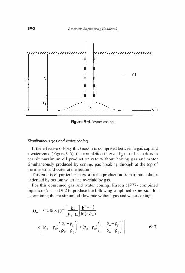
If the effective oil-pay thickness h is comprised between a gas cap anda water zone (Figure 9-5), the completion interval hp must be such as topermit maximum oil-production rate without having gas and watersimultaneously produced by coning, gas breaking through at the top ofthe interval and water at the bottom.
This case is of particular interest in the production from a thin columnunderlaid by bottom water and overlaid by gas.
For this combined gas and water coning, Pirson (1977) combinedEquations 9-1 and 9-2 to produce the following simplified expression fordetermining the maximum oil flow rate without gas and water coning:
oc4 o
o o
2p
e w
w o
o g
w
Q = 0.246 10k
B
h h
r r
( )
× ⎡⎣⎢
⎤⎦⎥
−( )
× −−
−
μ
ρ ρρ ρ
2
2
ln /
ρρ ρρ ρ
ρ ρρ ρ−
⎛⎝⎜
⎞⎠⎟
+ − −−−
⎛⎝⎜
⎞⎠⎟
⎡
⎣⎢⎢
⎤
⎦⎥⎥g
o g
o g
w g
( ) 1
2
(9-3)
590 Reservoir Engineering Handbook
Figure 9-4. Water coning.
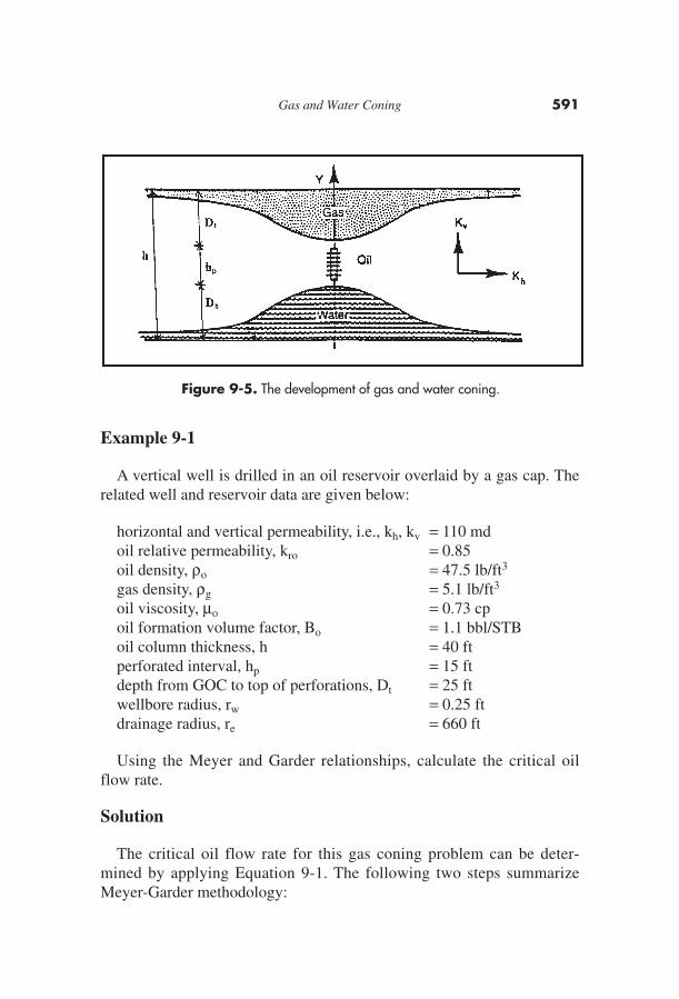
Example 9-1
A vertical well is drilled in an oil reservoir overlaid by a gas cap. Therelated well and reservoir data are given below:
horizontal and vertical permeability, i.e., kh, kv = 110 mdoil relative permeability, kro = 0.85oil density, ρo = 47.5 lb/ft3
gas density, ρg = 5.1 lb/ft3
oil viscosity, μo = 0.73 cpoil formation volume factor, Bo = 1.1 bbl/STBoil column thickness, h = 40 ftperforated interval, hp = 15 ftdepth from GOC to top of perforations, Dt = 25 ftwellbore radius, rw = 0.25 ftdrainage radius, re = 660 ft
Using the Meyer and Garder relationships, calculate the critical oilflow rate.
Solution
The critical oil flow rate for this gas coning problem can be deter-mined by applying Equation 9-1. The following two steps summarizeMeyer-Garder methodology:
Gas and Water Coning 591
Figure 9-5. The development of gas and water coning.
Step 1. Calculate effective oil permeability ko:
ko = kro k = (0.85) (110) = 93.5 md
Step 2. Solve for Qoc by applying Equation 9-1:
Example 9-2
Resolve Example 9-1 assuming that the oil zone is underlaid by bot-tom water. The water density is given as 63.76 lb/ft3. The well comple-tion interval is 15 feet as measured from the top of the formation (no gascap) to the bottom of the perforations.
Solution
The critical oil flow rate for this water coning problem can be estimatedby applying Equation 9-2. The equation is designed to determine the criti-cal rate at which the water cone “touches” the bottom of the well to give
The above two examples signify the effect of the fluid density differ-ences on critical oil flow rate.
Example 9-3
A vertical well is drilled in an oil reservoir that is overlaid by a gas capand underlaid by bottom water. Figure 9-6 shows an illustration of thesimultaneous gas and water coning.
oc2 2
oc
Q = 0.24663.76 47.5
l (660 / 0.25)93.5
(0.73)(1.1)40 15
Q = 8.13 STB/day
× −⎡⎣⎢
⎤⎦⎥
⎛⎝⎜
⎞⎠⎟
−−10 4 ( )n
[ ]
oc2 2Q = 0.246
47.5 5.1l (660/0.25)
93.5(0.73)(1.1)
40 (40 25)
= 21.20 STB/day
× − − −−10 4
n[ ]
592 Reservoir Engineering Handbook
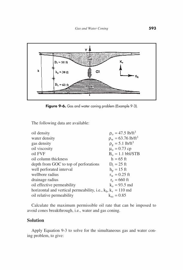
The following data are available:
oil density ρo = 47.5 lb/ft3
water density ρw = 63.76 lb/ft3
gas density ρg = 5.1 lb/ft3
oil viscosity μo = 0.73 cpoil FVF Bo = 1.1 bbl/STBoil column thickness h = 65 ftdepth from GOC to top of perforations Dt = 25 ftwell perforated interval hp = 15 ftwellbore radius rw = 0.25 ftdrainage radius re = 660 ftoil effective permeability ko = 93.5 mdhorizontal and vertical permeability, i.e., kh, kv = 110 mdoil relative permeability kro = 0.85
Calculate the maximum permissible oil rate that can be imposed toavoid cones breakthrough, i.e., water and gas coning.
Solution
Apply Equation 9-3 to solve for the simultaneous gas and water con-ing problem, to give:
Gas and Water Coning 593
Figure 9-6. Gas and water coning problem (Example 9-3).
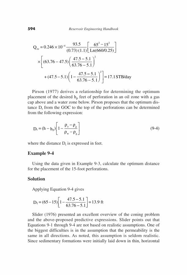
Pirson (1977) derives a relationship for determining the optimumplacement of the desired hp feet of perforation in an oil zone with a gascap above and a water zone below. Pirson proposes that the optimum dis-tance Dt from the GOC to the top of the perforations can be determinedfrom the following expression:
where the distance Dt is expressed in feet.
Example 9-4
Using the data given in Example 9-3, calculate the optimum distancefor the placement of the 15-foot perforations.
Solution
Applying Equation 9-4 gives
Slider (1976) presented an excellent overview of the coning problemand the above-proposed predictive expressions. Slider points out thatEquations 9-1 through 9-4 are not based on realistic assumptions. One ofthe biggest difficulties is in the assumption that the permeability is thesame in all directions. As noted, this assumption is seldom realistic.Since sedimentary formations were initially laid down in thin, horizontal
tD = (65 15) 147.5 5.1
63.76 5.1= 13.9 ft− − −
−⎡⎣⎢
⎤⎦⎥
t po g
w g
D = (h h ) 1− −−−
⎡
⎣⎢
⎤
⎦⎥
ρ ρρ ρ
(9-4)
oc
2 2
Q = 0.24693.5
(0.73) (1.1)65 15(660/0.25)
(63
× −⎡⎣⎢
⎤⎦⎥
×
−10 4
Ln
..76 47.5)
+ (47.5 5.1) 147.5 2
− −−
⎛⎝⎜
⎞⎠⎟
⎡
⎣⎢
− −
47 5 5 1
63 76 5 1
2. .
. .
−−−
⎛⎝⎜
⎞⎠⎟
⎤
⎦⎥ =5.1
63.76 5. 17.1 STB/day
1
594 Reservoir Engineering Handbook
sheets, it is natural for the formation permeability to vary from one sheetto another vertically.
Therefore, there is generally quite a difference between the permeabil-ity measured in a vertical direction and the permeability measured in ahorizontal direction. Furthermore, the permeability in the horizontaldirection is normally considerably greater than the permeability in thevertical direction. This also seems logical when we recognize that verythin, even microscopic sheets of impermeable material, such as shale,may have been periodically deposited. These permeability barriers have agreat effect on the vertical flow and have very little effect on the horizon-tal flow, which would be parallel to the plane of the sheets.
The Chierici-Ciucci Approach
Chierici and Ciucci (1964) used a potentiometric model to predict theconing behavior in vertical oil wells. The results of their work are pre-sented in dimensionless graphs that take into account the vertical andhorizontal permeability. The diagrams can be used for solving the follow-ing two types of problems:
a. Given the reservoir and fluid properties, as well as the position of andlength of the perforated interval, determine the maximum oil produc-tion rate without water and/or gas coning.
b. Given the reservoir and fluids characteristics only, determine the opti-mum position of the perforated interval.
The authors introduced four dimensionless parameters that can be deter-mined from a graphical correlation to determine the critical flow rates.The proposed four dimensionless parameters are shown in Figure 9-7 anddefined as follows:
Effective dimensionless radius rDe:
The first dimensionless parameter that the authors used to correlateresults of potentiometric model is called the effective dimensionlessradius and is defined by:
rr
h
k
kDe
e h
v
= (9-5)
Gas and Water Coning 595
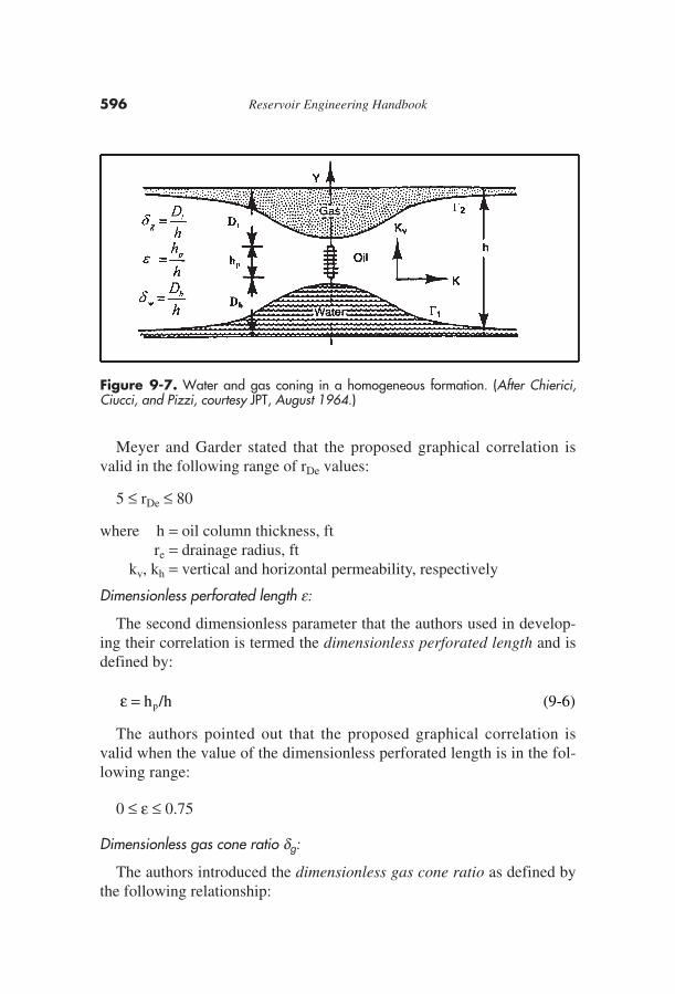
Meyer and Garder stated that the proposed graphical correlation isvalid in the following range of rDe values:
5 ≤ rDe ≤ 80
where h = oil column thickness, ftre = drainage radius, ft
kv, kh = vertical and horizontal permeability, respectively
Dimensionless perforated length e:
The second dimensionless parameter that the authors used in develop-ing their correlation is termed the dimensionless perforated length and isdefined by:
The authors pointed out that the proposed graphical correlation isvalid when the value of the dimensionless perforated length is in the fol-lowing range:
0 ≤ ε ≤ 0.75
Dimensionless gas cone ratio dg:
The authors introduced the dimensionless gas cone ratio as defined bythe following relationship:
ε = h hp/ (9-6)
596 Reservoir Engineering Handbook
Figure 9-7. Water and gas coning in a homogeneous formation. (After Chierici,Ciucci, and Pizzi, courtesy JPT, August 1964.)
with
0.070 ≤ δg ≤ 0.9
where Dt is the distance from the original GOC to the top of perfora-tions, ft.
Dimensionless water cone ratio dw:
The last dimensionless parameter that Chierici et al. proposed indeveloping their correlation is called the dimensionless water cone ratioand is defined by:
with
0.07 ≤ δw ≤ 0.9
where Db = distance from the original WOC to the bottom of theperforations, ft
Chierici and coauthors proposed that the oil-water and gas-oil contactsare stable only if the oil production rate of the well is not higher than thefollowing rates:
where Qow = critical oil flow rate in oil-water system, STB/dayQog = critical oil flow rate in gas-oil system, STB/day
ρo, ρw, ρg = densities in lb/ft3
ψw = water dimensionless functionψg = gas dimensionless functionkh = horizontal permeability, md
og
2o g
o o
ro h g De gQ = 0.492h ( )
B (k k ) (r , , )×
−−10 4
ρ ρμ
ε δΨ (9-10)
ow
2w o
o o
ro h w De wQ = 0.492 h ( )
B(k k ) (r , , )×
−−10 4 ρ ρμ
ψ ε δ (9-9)
w b= D /hδ (9-8)
g t= D /hδ (9-7)
Gas and Water Coning 597
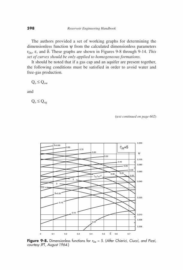
The authors provided a set of working graphs for determining thedimensionless function ψ from the calculated dimensionless parametersrDe, ε, and δ. These graphs are shown in Figures 9-8 through 9-14. Thisset of curves should be only applied to homogeneous formations.
It should be noted that if a gas cap and an aquifer are present together,the following conditions must be satisfied in order to avoid water andfree-gas production.
Qo ≤ Qow
and
Qo ≤ Qog
598 Reservoir Engineering Handbook
0.006
0.008
0.010
0.020
0.040
0.060
0.080
0.200
0.800.70
0.60
0.50
0.40
0.35
0.30
0.25
0.100
0 0.1 0.2 0.3 0.4 0.5 0.6 0.7
0.07
0.10
0.15
4
3
2
0.250.50
ψ
0=0.90
0=0.20
ρog ρwo=1
DE=5
ε
Figure 9-8. Dimensionless functions for rDe = 5. (After Chierici, Ciucci, and Pizzi,courtesy JPT, August 1964.)
(text continued on page 602)
0.006
0.008
0.010
0.020
0.040
0.060
0.080
0.200
0.800.70
0.60
0.50
0.40
0.35
0.30
0.25
0.100
0 0.1 0.2 0.3 0.4 0.5 0.6 0.7
0.07
0.10
0.15
4
3
2
0.250.50 ρog
ψ0=0.90 DE=10
ρog ρwo=1
0=0.20
ε
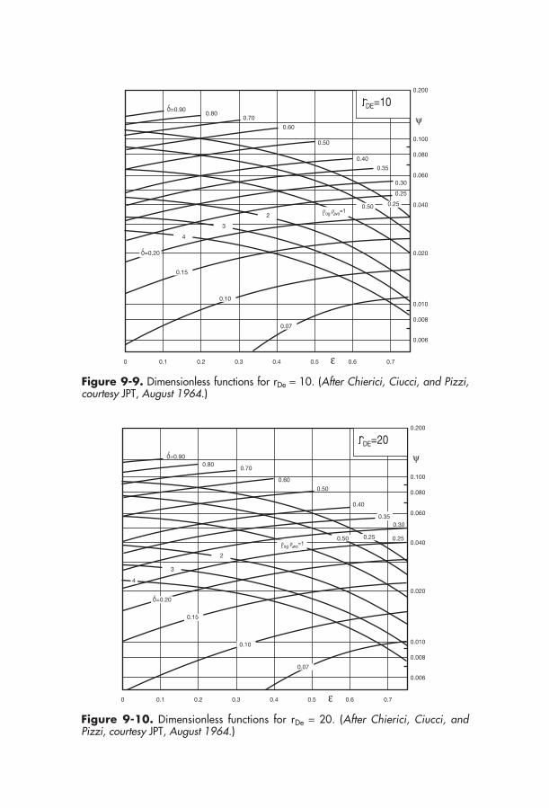
Figure 9-9. Dimensionless functions for rDe = 10. (After Chierici, Ciucci, and Pizzi,courtesy JPT, August 1964.)
0.006
0.008
0.010
0.020
0.040
0.060
0.080
0.200
0.800.70
0.60
0.50
0.40
0.30
0.25
0.100
0 0.1 0.2 0.3 0.4 0.5 0.6 0.7
0.07
0.10
0.15
4
3
2
0.250.50
ψ
0.35
0=0.90
0=0.20
ρog ρwo=1
DE=20
ε
Figure 9-10. Dimensionless functions for rDe = 20. (After Chierici, Ciucci, andPizzi, courtesy JPT, August 1964.)
600 Reservoir Engineering Handbook
0.006
0.008
0.010
0.020
0.040
0.060
0.080
0.200
0.80 0.70
0.60
0.50
0.40
0.30
0.25
0.100
0 0.1 0.2 0.3 0.4 0.5 0.6 0.7
0.07
0.10
0.15
4
3
2
0.250.50
ψ
0.35
0=0.90
0=0.20
ρog ρwo=1
DE=30
ε
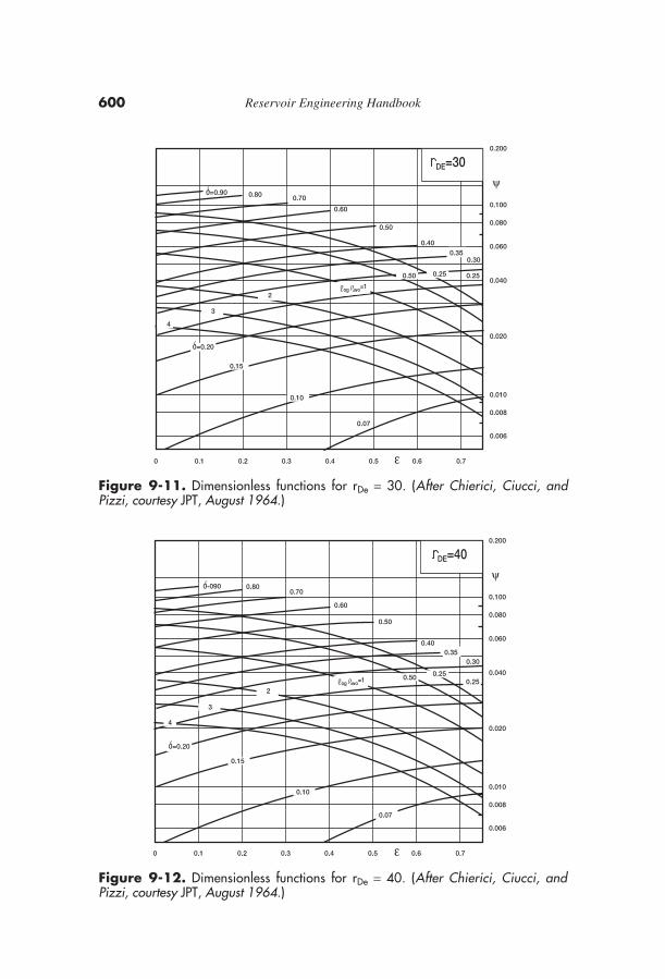
Figure 9-11. Dimensionless functions for rDe = 30. (After Chierici, Ciucci, andPizzi, courtesy JPT, August 1964.)
0.006
0.008
0.010
0.020
0.040
0.060
0.080
0.200
0.800.70
0.60
0.50
0.40
0.30
0.100
0 0.1 0.2 0.3 0.4 0.5 0.6 0.7
0.07
0.10
0.15
4
3
2
0.250.50
ψ
0.35
0.25
0-090
0=0.20
ρog ρwo=1
DE=40
ε
Figure 9-12. Dimensionless functions for rDe = 40. (After Chierici, Ciucci, andPizzi, courtesy JPT, August 1964.)
Gas and Water Coning 601
0.006
0.008
0.010
0.020
0.040
0.060
0.080
0.200
0.700.60
0.50
0.40
0.30
0.100
0 0.1 0.2 0.3 0.4 0.5 0.6 0.7
0.07
0.10
0.15
4
3
2
0.250.50
ψ
0.35
0.25
0.800=0.90
0=0.20
ρog ρwo=1
DE=60
ε
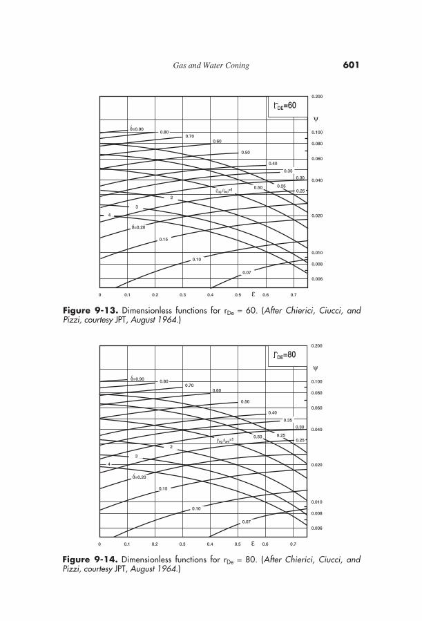
Figure 9-13. Dimensionless functions for rDe = 60. (After Chierici, Ciucci, andPizzi, courtesy JPT, August 1964.)
0.006
0.008
0.010
0.020
0.040
0.060
0.080
0.200
0.700.60
0.50
0.40
0.30
0.100
0 0.1 0.2 0.3 0.4 0.5 0.6 0.7
0.07
0.10
0.15
4
3
2
0.250.50
ψ
0.35
0.25
0.800=0.90
0=0.20
ρog ρwo=1
DE=80
ε
Figure 9-14. Dimensionless functions for rDe = 80. (After Chierici, Ciucci, andPizzi, courtesy JPT, August 1964.)
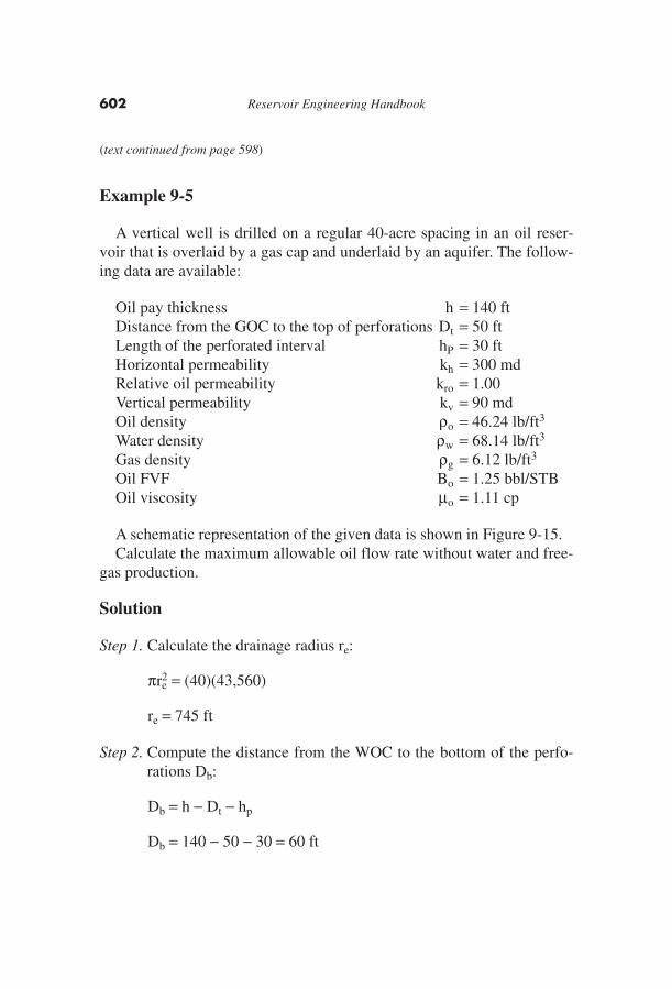
Example 9-5
A vertical well is drilled on a regular 40-acre spacing in an oil reser-voir that is overlaid by a gas cap and underlaid by an aquifer. The follow-ing data are available:
Oil pay thickness h = 140 ftDistance from the GOC to the top of perforations Dt = 50 ftLength of the perforated interval hP = 30 ftHorizontal permeability kh = 300 mdRelative oil permeability kro = 1.00Vertical permeability kv = 90 mdOil density ρo = 46.24 lb/ft3
Water density ρw = 68.14 lb/ft3
Gas density ρg = 6.12 lb/ft3
Oil FVF Bo = 1.25 bbl/STBOil viscosity μo = 1.11 cp
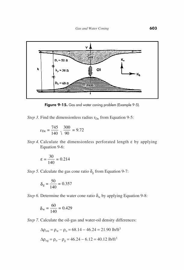
A schematic representation of the given data is shown in Figure 9-15.Calculate the maximum allowable oil flow rate without water and free-
gas production.
Solution
Step 1. Calculate the drainage radius re:
πre2 = (40)(43,560)
re = 745 ft
Step 2. Compute the distance from the WOC to the bottom of the perfo-rations Db:
Db = h − Dt − hp
Db = 140 − 50 − 30 = 60 ft
602 Reservoir Engineering Handbook
(text continued from page 598)
Step 3. Find the dimensionless radius rDe from Equation 9-5:
Step 4. Calculate the dimensionless perforated length ε by applyingEquation 9-6:
Step 5. Calculate the gas cone ratio δg from Equation 9-7:
Step 6. Determine the water cone ratio δw by applying Equation 9-8:
Step 7. Calculate the oil-gas and water-oil density differences:
Δρow = ρw − ρo = 68.14 − 46.24 = 21.90 lb/ft3
Δρog = ρo − ρg = 46.24 − 6.12 = 40.12 lb/ft3
w =60
140= 0.429δ
g =50
140= 0.357δ
ε =30
140= 0.214
Der =745140
30090
= 9.72
Gas and Water Coning 603
Figure 9-15. Gas and water coning problem (Example 9-5).
Step 8. Find the density differences ratio:
Step 9. From Figure 9-10, which corresponds to rDe = 10; approximatethe dimensionless functions ψg and ψw:
for ε = 0.214 and δg = 0.357 to give ψg = 0.051
and
for ε = 0.214 and δw = 0.429 to give ψw = 0.065
Step 10. Estimate the oil critical rate by applying Equations 9-9 and 9-10:
These calculations show that the water coning is the limiting conditionfor the oil flow rate. The maximum oil rate without water or free-gas pro-duction is, therefore, 297 STB/day.
Chierici and Ciucci (1964) proposed a methodology for determiningthe optimum completion interval in coning problems. The method isbasically based on the “trial and error” approach.
For a given dimensionless radius rDe and knowing GOC, WOC, andfluids density, the specific steps of the proposed methodology are sum-marized below:
Step 1. Assume the length of the perforated interval hp.
Step 2. Calculate the dimensionless perforated length ε = hp/h.
Step 3. Select the appropriate family of curves that corresponds to rDe,interpolate if necessary, and enter the working charts with ε onthe x-axis and move vertically to the calculated ratio Δρog/Δρow.Estimate the corresponding δ and ψ. Designate these two dimen-
ow
2
og
2
Q = 0.492140 (21.90)
(1.25) (1.11)(1) (300) STB day
Q = 0.492140 (40.12)
(1.25) (1.11) (1) (300) 0.051 = 426 STB/day
× =
×
−
−
10 0 065 97
10
4
4
[ ] . /
[ ]
2
Δ Δog ow/ =40.1221.90
= 1.83ρ ρ
604 Reservoir Engineering Handbook
sionless parameters as the optimum gas cone ratio δg,opt and opti-mum dimensionless function ψopt.
Step 4. Calculate the distance from GOC to the top of the perforation,
Dt = (h) (δg,opt)
Step 5. Calculate the distance from the WOC to the bottom of the perfo-ration, hw,
Db = h − Dt − hp
Step 6. Using the optimum dimensionless function ψopt in Equation 9-9,calculate the maximum allowable oil flow rate Qow.
Step 7. Repeat Steps 1 through 6.
Step 8. The calculated values of Qow at different assumed perforated inter-vals should be compared with those obtained from flow-rate equa-tions, e.g., Darcy’s equation, using the maximum drawdown pres-sure.
Example 9-6
Example 9-5 indicates that a vertical well is drilled in an oil reservoirthat is overlaid by a gas cap and underlaid by an aquifer. Assuming thatthe pay thickness h is 200 feet and the rock and fluid properties are iden-tical to those given in Example 9-5, calculate length and position of theperforated interval.
Solution
Step 1. Using the available data, calculate
r745
200
300
90= 6.8
and
/ = 40.12 / 21.90
De
og wo
=
Δ Δρ ρ == 1.83
Gas and Water Coning 605
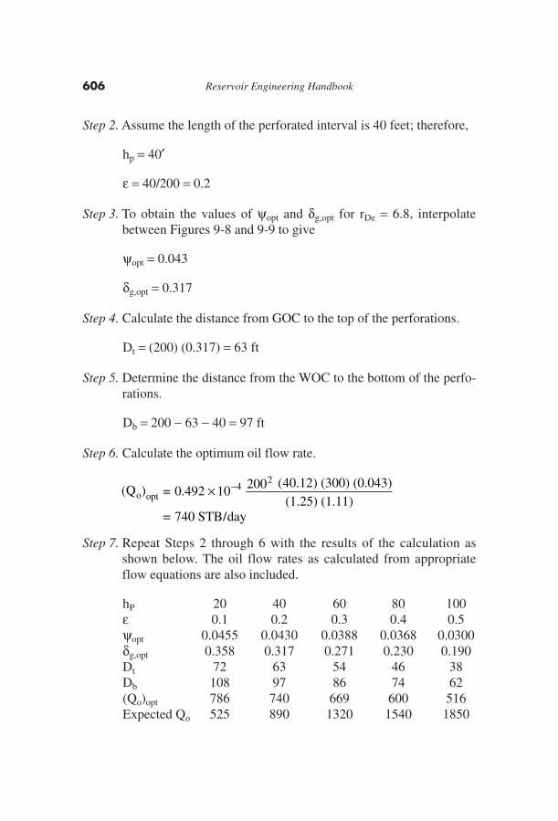
Step 2. Assume the length of the perforated interval is 40 feet; therefore,
hp = 40′
ε = 40/200 = 0.2
Step 3. To obtain the values of ψopt and δg,opt for rDe = 6.8, interpolatebetween Figures 9-8 and 9-9 to give
ψopt = 0.043
δg,opt = 0.317
Step 4. Calculate the distance from GOC to the top of the perforations.
Dt = (200) (0.317) = 63 ft
Step 5. Determine the distance from the WOC to the bottom of the perfo-rations.
Db = 200 − 63 − 40 = 97 ft
Step 6. Calculate the optimum oil flow rate.
Step 7. Repeat Steps 2 through 6 with the results of the calculation asshown below. The oil flow rates as calculated from appropriateflow equations are also included.
hP 20 40 60 80 100ε 0.1 0.2 0.3 0.4 0.5ψopt 0.0455 0.0430 0.0388 0.0368 0.0300δg,opt 0.358 0.317 0.271 0.230 0.190Dt 72 63 54 46 38Db 108 97 86 74 62(Qo)opt 786 740 669 600 516Expected Qo 525 890 1320 1540 1850
opto
2(Q ) = 0.492 200 ( ) (300) (0.043)
(1.25) (1.11)= 740 STB/day
× −1040 124 .
606 Reservoir Engineering Handbook
The maximum oil production rate that can be obtained from thiswell without coning breakthrough is 740 STB/day. This indicatesthat the optimum distance from the GOC to the top of the perfora-tions is 63 ft and the optimum distance from the WOC to the bot-tom of the perforations is 97 ft. The total length of the perforatedinterval is 200 − 63 − 97 = 40 ft.
The Hoyland-Papatzacos-Skjaeveland Methods
Hoyland, Papatzacos, and Skjaeveland (1989) presented two methodsfor predicting critical oil rate for bottom water coning in anisotropic,homogeneous formations with the well completed from the top of theformation. The first method is an analytical solution, and the second is anumerical solution to the coning problem. A brief description of themethods and their applications are presented below.
The Analytical Solution Method
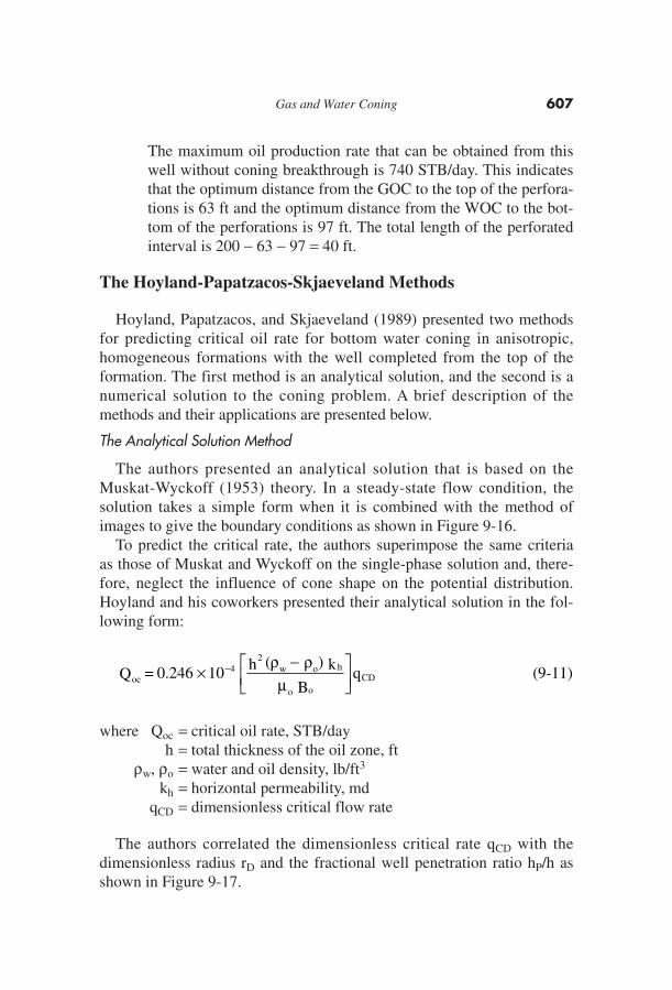
The authors presented an analytical solution that is based on theMuskat-Wyckoff (1953) theory. In a steady-state flow condition, thesolution takes a simple form when it is combined with the method ofimages to give the boundary conditions as shown in Figure 9-16.
To predict the critical rate, the authors superimpose the same criteriaas those of Muskat and Wyckoff on the single-phase solution and, there-fore, neglect the influence of cone shape on the potential distribution.Hoyland and his coworkers presented their analytical solution in the fol-lowing form:
where Qoc = critical oil rate, STB/dayh = total thickness of the oil zone, ft
ρw, ρo = water and oil density, lb/ft3
kh = horizontal permeability, mdqCD = dimensionless critical flow rate
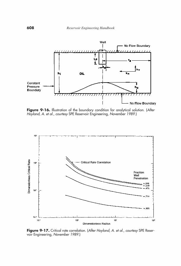
The authors correlated the dimensionless critical rate qCD with thedimensionless radius rD and the fractional well penetration ratio hP/h asshown in Figure 9-17.
oc
2w o h
o oCDQ = 0.246 h ( ) k
Bq×
−⎡⎣⎢
⎤⎦⎥
−10 4 ρ ρμ
(9-11)
Gas and Water Coning 607
608 Reservoir Engineering Handbook
Figure 9-16. Illustration of the boundary condition for analytical solution. (AfterHoyland, A. et al., courtesy SPE Reservoir Engineering, November 1989.)
Figure 9-17. Critical rate correlation. (After Hoyland, A. et al., courtesy SPE Reser-voir Engineering, November 1989.)

where re = drainage radius, ftkv = vertical permeability, mdkh = horizontal permeability, md
The Numerical Solution Method
Based on a large number of simulation runs with more than 50 criticalrate values, the authors used a regression analysis routine to develop thefollowing relationships:
• For isotropic reservoirs with kh = kv, the following expression is pro-posed:
• For anisotropic reservoirs, the authors correlated the dimensionless crit-ical rate with the dimensionless radius rD and five different fractionalwell penetrations. The correlation is presented in a graphical form asshown in Figure 9-18.
The authors illustrated their methodology through the following example.
Example 9-7
Given the following data, determine the oil critical rate:
Density differences (water/oil), lbm/ft3 = 17.4Oil FVF, RB/STB = 1.376Oil viscosity, cp = 0.8257Horizontal permeability, md = 1000Vertical permeability, md = 640Total oil thickness, ft = 200Perforated thickness, ft = 50External radius, ft = 500
oco w o
o o
P
2.238
Q = 0.924 k ( )
B1
h
h
h l
×−
− ⎛⎝ )⎡
⎣⎢⎤⎦⎥
×
−10 42 1 325
ρ ρμ
.
[ n (r )e1.99]− (9-13)
De v
hr = r
hk
k(9-12)
Gas and Water Coning 609
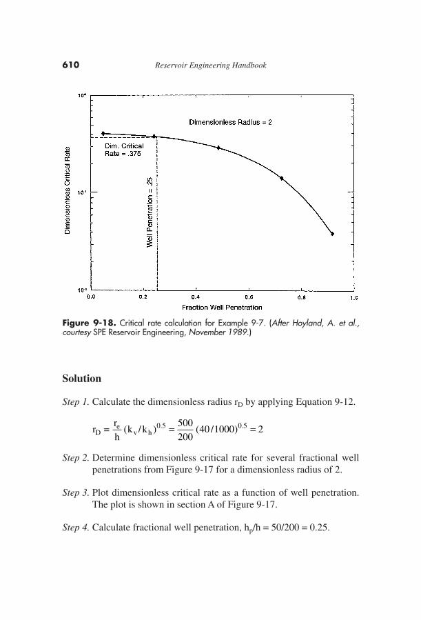
Solution
Step 1. Calculate the dimensionless radius rD by applying Equation 9-12.
Step 2. Determine dimensionless critical rate for several fractional wellpenetrations from Figure 9-17 for a dimensionless radius of 2.
Step 3. Plot dimensionless critical rate as a function of well penetration.The plot is shown in section A of Figure 9-17.
Step 4. Calculate fractional well penetration, hp/h = 50/200 = 0.25.
r =rh
k kDe
v h( / ) ( / ). .0 5 0 5500200
40 1000 2= =
610 Reservoir Engineering Handbook
Figure 9-18. Critical rate calculation for Example 9-7. (After Hoyland, A. et al.,courtesy SPE Reservoir Engineering, November 1989.)
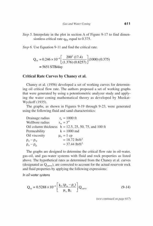
Step 5. Interpolate in the plot in section A of Figure 9-17 to find dimen-sionless critical rate qDc equal to 0.375.
Step 6. Use Equation 9-11 and find the critical rate.
Critical Rate Curves by Chaney et al.
Chaney et al. (1956) developed a set of working curves for determin-ing oil critical flow rate. The authors proposed a set of working graphsthat were generated by using a potentiometric analyzer study and apply-ing the water coning mathematical theory as developed by Muskat-Wyckoff (1935).
The graphs, as shown in Figures 9-19 through 9-23, were generatedusing the following fluid and sand characteristics:
Drainage radius re = 1000 ftWellbore radius rw = 3″Oil column thickness h = 12.5, 25, 50, 75, and 100 ftPermeability k = 1000 mdOil viscosity μo = 1 cpρo − ρw = 18.72 lb/ft3
ρo − ρg = 37.44 lb/ft3
The graphs are designed to determine the critical flow rate in oil-water,gas-oil, and gas-water systems with fluid and rock properties as listedabove. The hypothetical rates as determined from the Chaney et al. curves(designated as Qcurve), are corrected to account for the actual reservoir rockand fluid properties by applying the following expressions:
In oil-water systems
oco w o
o ocurveQ = 0.5288 k ( )
BQ×
−⎡⎣⎢
⎤⎦⎥
−10 4 ρ ρμ
(9-14)
Q =oc 0 246 10200 17 4
1 376 0 82571000 0 3754
2
.( . )
( . ) ( . )( ) ( . )× ⎡
⎣⎢⎤⎦⎥
−
== 5651STB day/
Gas and Water Coning 611
(text continued on page 617)
612 Reservoir Engineering Handbook
0.1
1.0
0.2
0.4
0.6
0.8
1.0
2.0
4.0
6.0
8.0
10.0
20.0
40.0
60.0
80.0
100.0
2.5 5.0 7.5 10.0 12.5
abcd
e
E
D C
B A
Distance from Top Perforation to Topof Sand or Gas-Oil Contact–In Feet
Critical Production Rates–Reservoir bbl/day
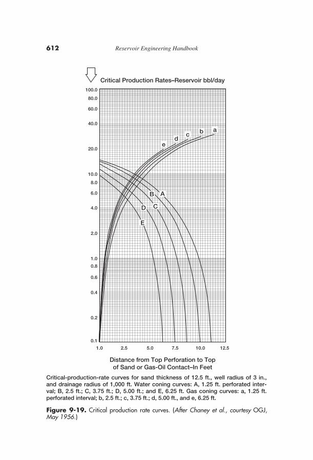
Figure 9-19. Critical production rate curves. (After Chaney et al., courtesy OGJ,May 1956.)
Critical-production-rate curves for sand thickness of 12.5 ft., well radius of 3 in.,and drainage radius of 1,000 ft. Water coning curves: A, 1.25 ft. perforated inter-val; B, 2.5 ft.; C, 3.75 ft.; D, 5.00 ft.; and E, 6.25 ft. Gas coning curves: a, 1.25 ft.perforated interval; b, 2.5 ft.; c, 3.75 ft.; d, 5.00 ft., and e, 6.25 ft.
Gas and Water Coning 613
0.1
0
0.2
0.4
0.6
0.81.0
2.0
4.0
6.0
8.010
20
40
60
80100
200
400
600
8001000
5 10 15 20 25
abcde
E
D C
B A
Distance from Top Perforation to Topof Sand or Gas-Oil Contact–In Feet
Critical Production Rates–Reservoir bbl/day
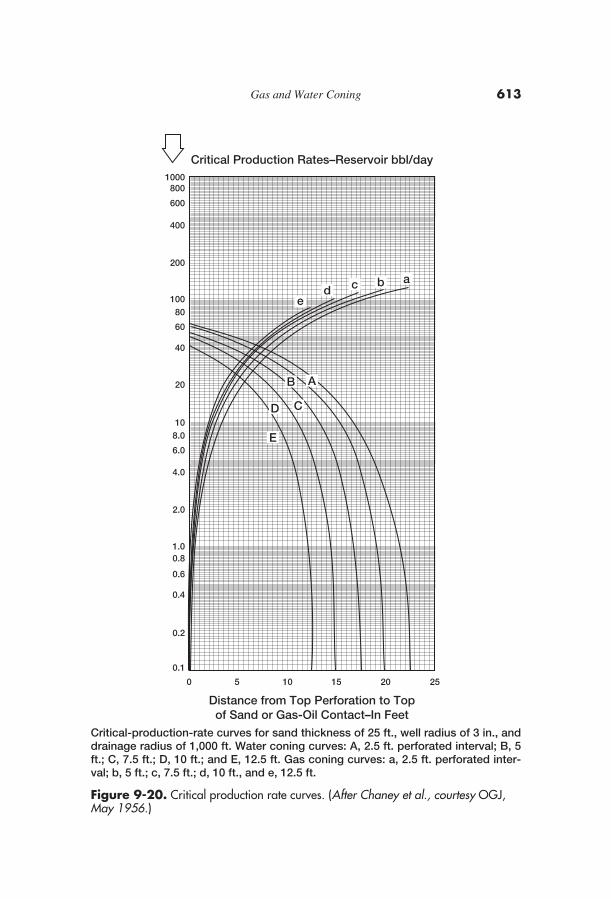
Figure 9-20. Critical production rate curves. (After Chaney et al., courtesy OGJ,May 1956.)
Critical-production-rate curves for sand thickness of 25 ft., well radius of 3 in., anddrainage radius of 1,000 ft. Water coning curves: A, 2.5 ft. perforated interval; B, 5ft.; C, 7.5 ft.; D, 10 ft.; and E, 12.5 ft. Gas coning curves: a, 2.5 ft. perforated inter-val; b, 5 ft.; c, 7.5 ft.; d, 10 ft., and e, 12.5 ft.

614 Reservoir Engineering Handbook
0.1
0
0.2
0.4
0.6
0.81.0
2.0
4.0
6.0
8.010
20
40
60
80100
200
400
600
8001000
10 20 30 40 50
abcd
e
E D
C B
A
Distance from Top Perforation to Topof Sand or Gas-Oil Contact–In Feet
Critical Production Rates–Reservoir bbl/day
Figure 9-21. Critical production rate curves. (After Chaney et al., courtesy OGJ,May 1956.)
Critical-production-rate curves for sand thickness of 50 ft., well radius of 3 in., anddrainage radius of 1,000 ft. Water coning curves: A, 5 ft. perforated interval; B, 10ft.; C, 15 ft.; D, 20 ft.; and E, 25 ft. Gas coning curves: a, 5 ft. perforated interval; b,10 ft.; c, 15 ft.; d, 20 ft., and e, 25 ft.
Gas and Water Coning 615
1.0
0
2.0
4.0
6.0
8.010
20
40
60
80100
200
400
600
8001000
2000
4000
6000
800010000
15 30 45 60 75
abcde
E D
C B
A
Distance fom Top Perforation to Topof Sand or Gas-Oil Contact–In Feet
Critical Production Rates–Reservoir bbl/day
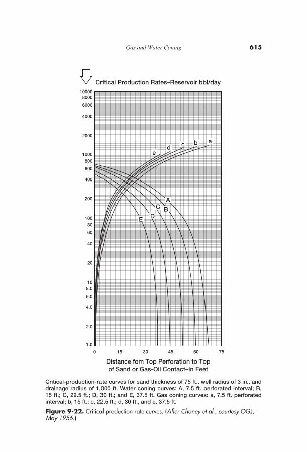
Figure 9-22. Critical production rate curves. (After Chaney et al., courtesy OGJ,May 1956.)
Critical-production-rate curves for sand thickness of 75 ft., well radius of 3 in., anddrainage radius of 1,000 ft. Water coning curves: A, 7.5 ft. perforated interval; B,15 ft.; C, 22.5 ft.; D, 30 ft.; and E, 37.5 ft. Gas coning curves: a, 7.5 ft. perforatedinterval; b, 15 ft.; c, 22.5 ft.; d, 30 ft., and e, 37.5 ft.

616 Reservoir Engineering Handbook
1.0
0
2.0
4.0
6.0
8.010
20
40
60
80100
200
400
600
8001000
2000
4000
6000
800010000
20 40 60 80 100
abcde
E
D C
B A
Distance from Top Perforation to Topof Sand or Gas-Oil Contact–In Feet
Critical Production Rates–Reservoir bbl/day
Figure 9-23. Critical production rate curves. (After Chaney et al., courtesy OGJ,May 1956.)
Critical-production-rate curves for sand thickness of 100 ft., well radius of 3 in.,and drainage radius of 1,000 ft. Water coning curves: A, 10 ft. perforated interval;B, 20 ft.; C, 30 ft.; D, 40 ft.; and E, 50 ft. Gas coning curves: a, 10 ft. perforatedinterval; b, 20 ft.; c, 30 ft.; d, 40 ft., and e, 50 ft.
where ρo = oil density, lb/ft3
ρw = water density, lb/ft3
Qoc = critical oil flow rate, STB/dayko = effective oil permeability, md
In gas-water systems
where ρg = gas density, lb/ft3
ρw = water density, lb/ft3
Qgc = critical gas flow rate, Mscf/dayβg = gas FVF, bbl/Mscfkg = effective gas permeability, md
In gas-oil systems
Example 9-8
In an oil-water system, the following fluid and sand data are available:
h = 50′ hp = 15′ρo = 47.5 lb/ft3 ρw = 63.76 lb/ft3
μo = 0.73 cp Bo = 1.1 bbl/STBrw = 3″ re = 1000′ko = 93.5 md
Calculate the oil critical rate.
Solution
Step 1. Distance from the top of the perforations to top of the sand = 0′
oc
o o g
o ocurveQ = 0.2676
k ( )
BQ×
−⎡⎣⎢
⎤⎦⎥
−10 4ρ ρ
μ(9-16)
gc
g w g
g gcurveQ = 0.5288
k ( )
BQ×
−⎡
⎣⎢
⎤
⎦⎥−10 4
ρ ρμ
(9-15)
Gas and Water Coning 617
(text continued from page 611)
Step 2. Using Figure 9-20, for h = 50, enter the graph with 0′ and movevertically to curve C to give:
Qcurve = 270 bbl/day
Step 3. Calculate critical oil rate from Equation 9-14.
The above method can be used through the trial-and-error procedure tooptimize the location of the perforated interval in two-cone systems. Itshould be pointed out that Chaney’s method was developed for a homo-geneous, isotropic reservoir with kv = kh.
Chaperson’s Method
Chaperson (1986) proposed a simple relationship to estimate the criti-cal rate of a vertical well in an anisotropic formation (kv ≠ kh). The rela-tionship accounts for the distance between the production well andboundary. The proposed correlation has the following form:
where Qoc = critical oil rate, STB/daykh = horizontal permeability, md
Δρ = ρw − ρo, density difference, lb/ft3
h = oil column thickness, fthp = perforated interval, ft
Joshi (1991) correlated the coefficient q*c with the parameter α″ as
q*c = 0.7311 + (1.943/α″) (9-18)
′′ = ( )α r h k ke v h/ / ( )9 19-
och
2p
o ocQ = 0.0783 k (h h )
B[ ] q×
−−10 9 174
μρΔ * ( )-
ocQ = 0.528893.5 (63.76 47.5)
(1.1) (0.73)270 = 27 STB/day× −⎡
⎣⎢
⎤
⎦⎥
−10 4
618 Reservoir Engineering Handbook
Example 9-9
The following data are available on an oil-water system:
h = 50′ re = 1000′ μo = 0.73 cpBo = 1.1 bbl/STB ρw = 63.76 lb/ft3 kh = 100 mdρo = 47.5 lb/ft3 kv = 10 md hP = 15′
Calculate the critical rate.
Solution
Step 1. Calculate α″ from Equation 9-19.
Step 2. Solve for q*c by applying Equation 9-18.
q*c = 0.7311 + (1.943/6.324) = 1.0383
Step 3. Solve for the critical oil rate Qoc by using Equation 9-17.
Schols’ Method
Schols (1972) developed an empirical equation based on resultsobtained from numerical simulator and laboratory experiments. His criti-cal rate equation has the following form:
ocw o o
2p2
o o
e
Q = 0.0783( ) k (h h )
u B
0.432 +3.142
l (
×− −⎡
⎣⎢⎤⎦⎥
×
−10 4 ρ ρ
n rr /r )(h/r )
w
0.14e
⎡⎣⎢
⎤⎦⎥
(9-20)
oc
2
oc
Q = 0.0783(100) (50 15)
(0.73) (1.1)[63.76 47.5] (1.0383)
Q = 20.16 STB/day
× − −−10 4
′′α = (1000/50) 10 /100 = 6.324
Gas and Water Coning 619
where ko = effective oil permeability, mdrw = wellbore radius, fthp = perforated interval, ftρ = density, lb/ft3
Schols’ equation is only valid for isotropic formation, i.e., kh = kv.
Example 9-10
In an oil-water system, the following fluid and rock data are available:
h = 50′ hp = 15′ ρo = 47.5 lb/ft3 ρw = 63.76 lb/ft3
μo = 0.73 cp Bo = 1.1 bbl/STB re = 1000′ rw = 0.25′ko = k = 93.5 md
Calculate the critical oil flow rate.
Solution
Applying Equation 9-20 gives
BREAKTHROUGH TIME IN VERTICAL WELLS
Critical flow rate calculations frequently show low rates that, for eco-nomic reasons, cannot be imposed on production wells. Therefore, if awell produces above its critical rate, the cone will break through after agiven time period. This time is called time to breakthrough tBT. Two ofthe most widely used correlations are documented below.
The Sobocinski-Cornelius Method
Sobocinski and Cornelius (1965) developed a correlation for predict-ing water breakthrough time based on laboratory data and modelingresults. The authors correlated the breakthrough time with two dimen-
oc
2 2
.14
oc
Q = 0.0783(63.76 47.5) (93.5) (50 15 )
(0.73) (1.1)
0.432 +3.142
l (1000 /.25)(50/1000 )
Q = 18 STB/day
× − −⎡
⎣⎢
⎤
⎦⎥
× ⎡⎣⎢
⎤⎦⎥
−10 4
0
n
620 Reservoir Engineering Handbook
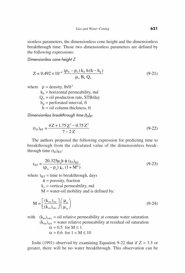
sionless parameters, the dimensionless cone height and the dimensionlessbreakthrough time. Those two dimensionless parameters are defined bythe following expressions:
Dimensionless cone height Z
where ρ = density, lb/ft3
kh = horizontal permeability, mdQo = oil production rate, STB/dayhp = perforated interval, fth = oil column thickness, ft
Dimensionless breakthrough time (tD)BT
The authors proposed the following expression for predicting time tobreakthrough from the calculated value of the dimensionless break-through time (tD)BT:
where tBT = time to breakthrough, daysφ = porosity, fraction
kv = vertical permeability, mdM = water-oil mobility and is defined by:
with (kro)swc = oil relative permeability at connate water saturation(krw)sor = water relative permeability at residual oil saturation
α = 0.5 for M ≤ 1α = 0.6 for 1 < M ≤ 10
Joshi (1991) observed by examining Equation 9-22 that if Z = 3.5 orgreater, there will be no water breakthrough. This observation can be
M =k
krw sor
ro swc
o
w
( )
( )⎡⎣⎢
⎤⎦⎥
⎛⎝⎜
⎞⎠⎟
μμ
(9-24)
t =20,325 h (t )
( ) k (1 + M )BT
o D BT
w o v
μ φρ ρ α−
(9-23)
( )t =4 Z 1.75 Z 0.75 Z
7 2 ZD BT
2+ −−
3
(9-22)
Z = 0.492k h h h
B Qw o h p
o o o
×− −−10 4 ( ) ( )ρ ρ
μ(9-21)
Gas and Water Coning 621
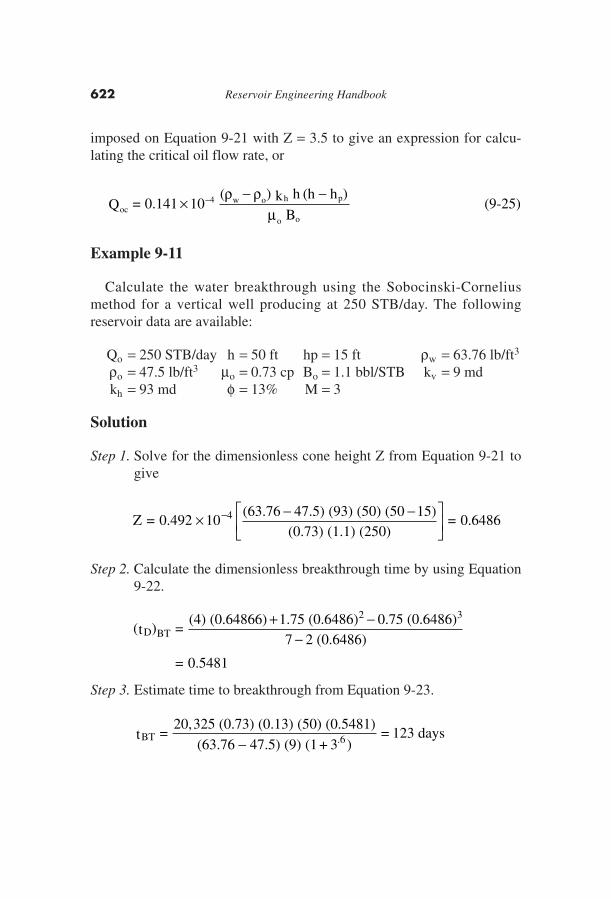
imposed on Equation 9-21 with Z = 3.5 to give an expression for calcu-lating the critical oil flow rate, or
Example 9-11
Calculate the water breakthrough using the Sobocinski-Corneliusmethod for a vertical well producing at 250 STB/day. The followingreservoir data are available:
Qo = 250 STB/day h = 50 ft hp = 15 ft ρw = 63.76 lb/ft3
ρo = 47.5 lb/ft3 μo = 0.73 cp Bo = 1.1 bbl/STB kv = 9 mdkh = 93 md φ = 13% M = 3
Solution
Step 1. Solve for the dimensionless cone height Z from Equation 9-21 togive
Step 2. Calculate the dimensionless breakthrough time by using Equation9-22.
Step 3. Estimate time to breakthrough from Equation 9-23.
BTt =20,325 (0.73) (0.13) (50) (0.5481)
(63.76 47.5) (9) (1 + )= 123 days
− 3 6.
BTD
2 3(t ) =
(4) (0.64866) 1.75 (0.6486) 0.75 (0.6486)7 2 (0.6486)
= 0.5481
+ −−
Z = 0.492(63.76 47.5) (93) (50) (50 15)
(0.73) (1.1) (250)= 0.6486× − −⎡
⎣⎢
⎤
⎦⎥
−10 4
ocw o h p
o o
Q = 0.141( ) k h (h h )
B×
− −−10 4 ρ ρμ
(9-25)
622 Reservoir Engineering Handbook

Example 9-12
Using the data given in Example 9-11, approximate the critical oilflow rate by using Equation 9-25.
Solution
The Bournazel-Jeanson Method
Based on experimental data, Bournazel and Jeanson (1971) developeda methodology that uses the same dimensionless groups proposed in theSobocinski-Cornelius method. The procedure of calculating the time tobreakthrough is given below.
Step 1. Calculate the dimensionless core height Z from Equation 9-21.
Step 2. Calculate the dimensionless breakthrough time by applying thefollowing expression:
Step 3. Solve for the time to breakthrough tBT by substituting the above-cal-culated dimensionless breakthrough time into Equation 9-23, i.e.,
As pointed out by Joshi (1991), Equation 9-26 indicates that nobreakthrough occurs if Z ≥ 4.286. Imposing this value on Equa-tion 9-21 gives a relationship for determining Qoc.
oc4 w o h p
o o
Q = 0.1148 10k h h h
B×
− −− ( ) ( )ρ ρμ
(9-27)
BTo D BT
w o vt =
20,325 h (t )
( ) k (1+ M )
μ φρ ρ α−
BTD(t ) =Z
3 0.7 Z−(9-26)
ocQ = 0.141(63.76 47.5) (93) (50) (50 15)
(0.73) (1.1)= 46.3 STB/day
× − −−10 4
Gas and Water Coning 623
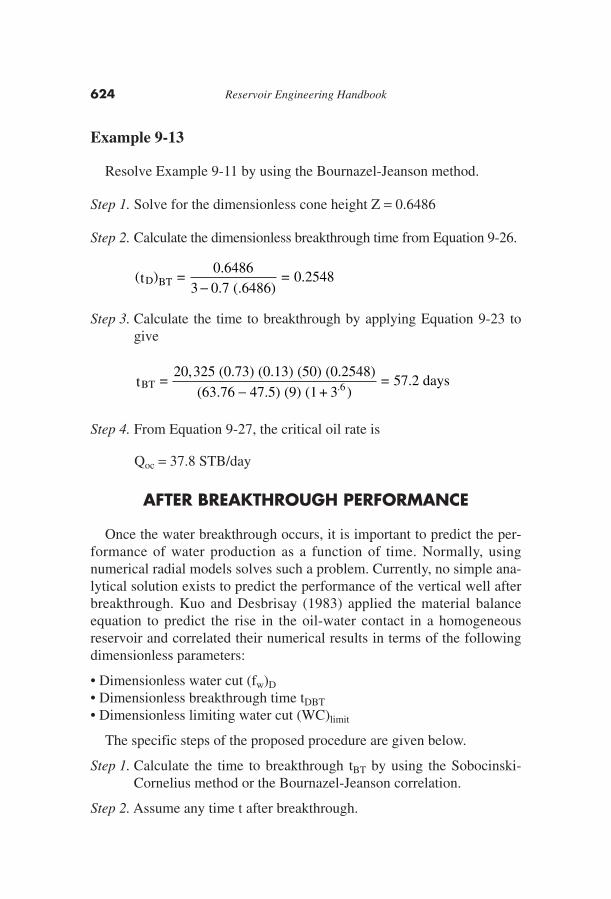
Example 9-13
Resolve Example 9-11 by using the Bournazel-Jeanson method.
Step 1. Solve for the dimensionless cone height Z = 0.6486
Step 2. Calculate the dimensionless breakthrough time from Equation 9-26.
Step 3. Calculate the time to breakthrough by applying Equation 9-23 togive
Step 4. From Equation 9-27, the critical oil rate is
Qoc = 37.8 STB/day
AFTER BREAKTHROUGH PERFORMANCE
Once the water breakthrough occurs, it is important to predict the per-formance of water production as a function of time. Normally, usingnumerical radial models solves such a problem. Currently, no simple ana-lytical solution exists to predict the performance of the vertical well afterbreakthrough. Kuo and Desbrisay (1983) applied the material balanceequation to predict the rise in the oil-water contact in a homogeneousreservoir and correlated their numerical results in terms of the followingdimensionless parameters:
• Dimensionless water cut (fw)D
• Dimensionless breakthrough time tDBT
• Dimensionless limiting water cut (WC)limit
The specific steps of the proposed procedure are given below.
Step 1. Calculate the time to breakthrough tBT by using the Sobocinski-Cornelius method or the Bournazel-Jeanson correlation.
Step 2. Assume any time t after breakthrough.
BTt =20,325 (0.73) (0.13) (50) (0.2548)
(63.76 47.5) (9) (1 + )= 57.2 days
− 3 6.
BTD(t ) =0.6486
3 0.7 (.6486)= 0.2548
−
624 Reservoir Engineering Handbook
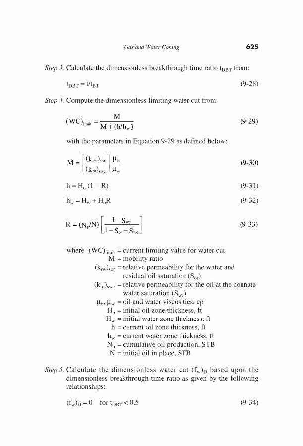
Step 3. Calculate the dimensionless breakthrough time ratio tDBT from:
tDBT = t/tBT (9-28)
Step 4. Compute the dimensionless limiting water cut from:
with the parameters in Equation 9-29 as defined below:
h = Ho (1 − R) (9-31)
hw = Hw + HoR (9-32)
where (WC)limit = current limiting value for water cutM = mobility ratio
(krw)sor = relative permeability for the water andresidual oil saturation (Sor)
(kro)swc = relative permeability for the oil at the connatewater saturation (Swc)
μo, μw = oil and water viscosities, cpHo = initial oil zone thickness, ftHw = initial water zone thickness, ft
h = current oil zone thickness, fthw = current water zone thickness, ftNp = cumulative oil production, STBN = initial oil in place, STB
Step 5. Calculate the dimensionless water cut (fw)D based upon thedimensionless breakthrough time ratio as given by the followingrelationships:
(fw)D = 0 for tDBT < 0.5 (9-34)
R = (N /N)1 S
1 S Sp
wc
or wc
−− −
⎡⎣⎢
⎤⎦⎥
(9-33)
M =(k )
(k )sorrw
swcro
o
w
⎡⎣⎢
⎤⎦⎥
μμ
(9-30)
WCM
M h hw
( ) =+ ( )limit (9-29)
/
Gas and Water Coning 625
(fw)D = 0.29 + 0.94 log (tDBT) for 0.5 ≤ tDBT ≤ 5.7 (9-35)
(fw)D = 1.0 for tDBT > 5.7 (9-36)
Step 6. Calculate the actual water cut fw from the expression:
fw = (fw)D (WC)limit (9-37)
Step 7. Calculate water and oil flow rate by using the following expres-sions:
Qw = (fw) QT (9-38)
Qo = QT − Qw (9-39)
where Qw, Qo, QT are the water, oil, and total flow rates,respectively.
It should be pointed out that as oil is recovered, the oil-water contactwill rise and the limiting value for water cut will change. It also shouldbe noted the limiting water cut value (WC)limit lags behind one time stepwhen calculating future water cut.
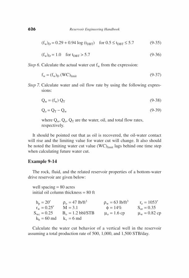
Example 9-14
The rock, fluid, and the related reservoir properties of a bottom-waterdrive reservoir are given below:
well spacing = 80 acresinitial oil column thickness = 80 ft
hp = 20′ ρo = 47 lb/ft3 ρw = 63 lb/ft3 re = 1053′rw = 0.25′ M = 3.1 φ = 14% Sor = 0.35
Swc = 0.25 Bo = 1.2 bbl/STB μo = 1.6 cp μw = 0.82 cpkh = 60 md kv = 6 md
Calculate the water cut behavior of a vertical well in the reservoirassuming a total production rate of 500, 1,000, and 1,500 STB/day.
626 Reservoir Engineering Handbook
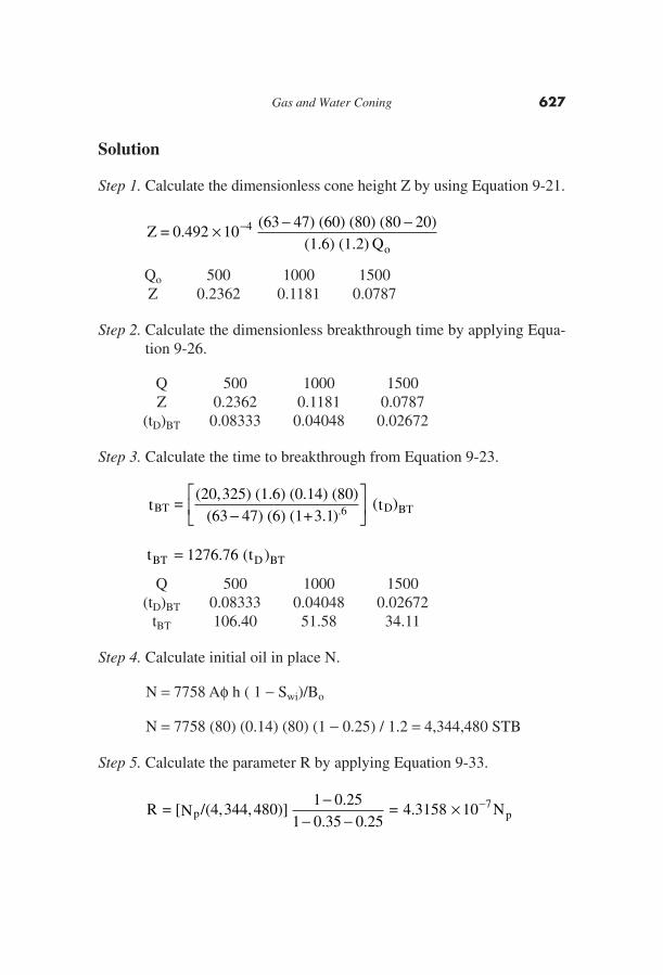
Solution
Step 1. Calculate the dimensionless cone height Z by using Equation 9-21.
Qo 500 1000 1500Z 0.2362 0.1181 0.0787
Step 2. Calculate the dimensionless breakthrough time by applying Equa-tion 9-26.
Q 500 1000 1500Z 0.2362 0.1181 0.0787
(tD)BT 0.08333 0.04048 0.02672
Step 3. Calculate the time to breakthrough from Equation 9-23.
Q 500 1000 1500(tD)BT 0.08333 0.04048 0.02672
tBT 106.40 51.58 34.11
Step 4. Calculate initial oil in place N.
N = 7758 Aφ h ( 1 − Swi)/Bo
N = 7758 (80) (0.14) (80) (1 − 0.25) / 1.2 = 4,344,480 STB
Step 5. Calculate the parameter R by applying Equation 9-33.
R = [N /(4,344,480)]1 0.25
1 0.35 0.25= 4.3158 Np p
−− −
× −10 7
BT .6 BTD
BT D BT
t =(20,325) (1.6) (0.14) (80)
(63 47) (6) (1+3.1) (t )
t t
−⎡
⎣⎢
⎤
⎦⎥
= 1276 76. ( )
Z = 0.492(63 47) (60) (80) (80 20)
(1.6) (1.2) Qo
× − −−10 4
Gas and Water Coning 627
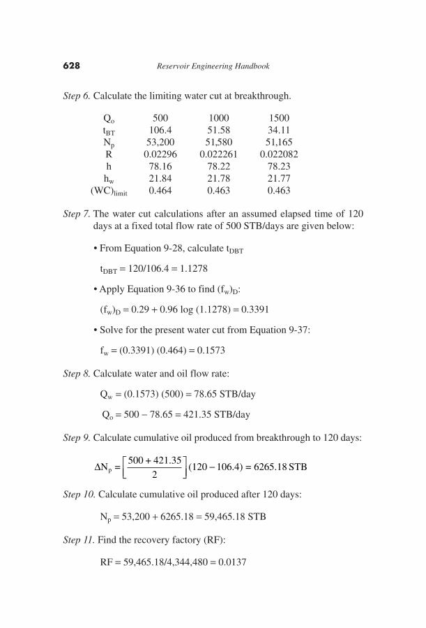
Step 6. Calculate the limiting water cut at breakthrough.
Qo 500 1000 1500tBT 106.4 51.58 34.11Np 53,200 51,580 51,165R 0.02296 0.022261 0.022082h 78.16 78.22 78.23
hw 21.84 21.78 21.77(WC)limit 0.464 0.463 0.463
Step 7. The water cut calculations after an assumed elapsed time of 120days at a fixed total flow rate of 500 STB/days are given below:
• From Equation 9-28, calculate tDBT
tDBT = 120/106.4 = 1.1278
• Apply Equation 9-36 to find (fw)D:
(fw)D = 0.29 + 0.96 log (1.1278) = 0.3391
• Solve for the present water cut from Equation 9-37:
fw = (0.3391) (0.464) = 0.1573
Step 8. Calculate water and oil flow rate:
Qw = (0.1573) (500) = 78.65 STB/day
Qo = 500 − 78.65 = 421.35 STB/day
Step 9. Calculate cumulative oil produced from breakthrough to 120 days:
Step 10. Calculate cumulative oil produced after 120 days:
Np = 53,200 + 6265.18 = 59,465.18 STB
Step 11. Find the recovery factory (RF):
RF = 59,465.18/4,344,480 = 0.0137
ΔN =500 + 421.35
2 (120 106.4) = 6265.18 STBp
⎡⎣⎢
⎤⎦⎥
−
628 Reservoir Engineering Handbook
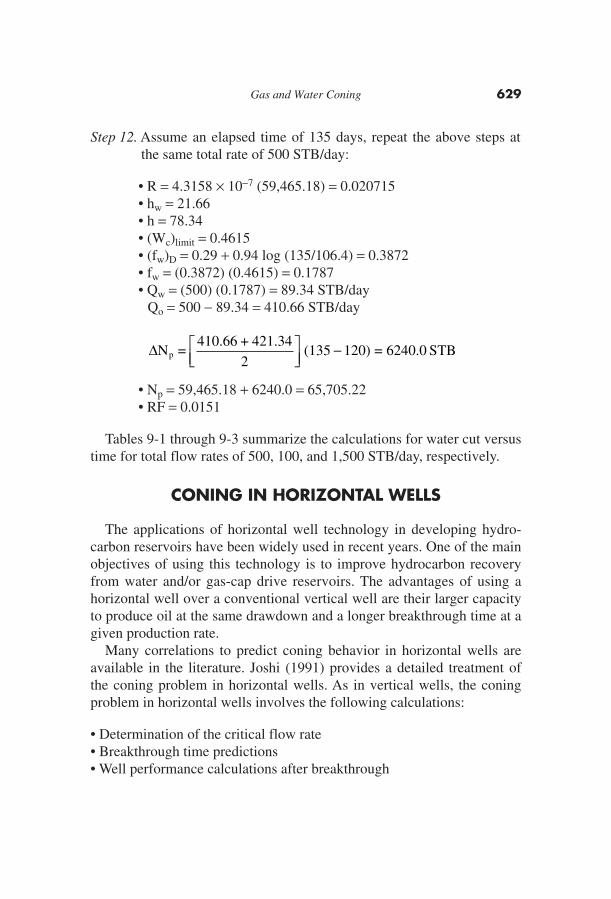
Step 12. Assume an elapsed time of 135 days, repeat the above steps atthe same total rate of 500 STB/day:
• R = 4.3158 × 10⁻⁷ (59,465.18) = 0.020715• hw = 21.66• h = 78.34• (Wc)limit = 0.4615• (fw)D = 0.29 + 0.94 log (135/106.4) = 0.3872• fw = (0.3872) (0.4615) = 0.1787• Qw = (500) (0.1787) = 89.34 STB/day
Qo = 500 − 89.34 = 410.66 STB/day
• Np = 59,465.18 + 6240.0 = 65,705.22• RF = 0.0151
Tables 9-1 through 9-3 summarize the calculations for water cut versustime for total flow rates of 500, 100, and 1,500 STB/day, respectively.
CONING IN HORIZONTAL WELLS
The applications of horizontal well technology in developing hydro-carbon reservoirs have been widely used in recent years. One of the mainobjectives of using this technology is to improve hydrocarbon recoveryfrom water and/or gas-cap drive reservoirs. The advantages of using ahorizontal well over a conventional vertical well are their larger capacityto produce oil at the same drawdown and a longer breakthrough time at agiven production rate.
Many correlations to predict coning behavior in horizontal wells areavailable in the literature. Joshi (1991) provides a detailed treatment ofthe coning problem in horizontal wells. As in vertical wells, the coningproblem in horizontal wells involves the following calculations:
• Determination of the critical flow rate• Breakthrough time predictions• Well performance calculations after breakthrough
ΔN =410.66 + 421.34
2(135 120) = 6240.0 STBp
⎡⎣⎢
⎤⎦⎥
−
Gas and Water Coning 629
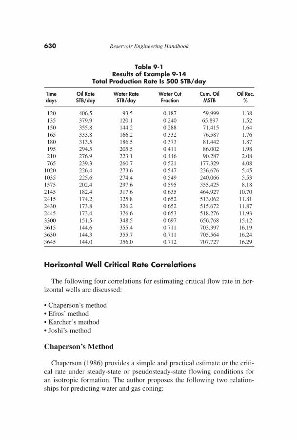
Table 9-1Results of Example 9-14
Total Production Rate Is 500 STB/day
Time Oil Rate Water Rate Water Cut Cum. Oil Oil Rec.days STB/day STB/day Fraction MSTB %
120 406.5 93.5 0.187 59.999 1.38135 379.9 120.1 0.240 65.897 1.52150 355.8 144.2 0.288 71.415 1.64165 333.8 166.2 0.332 76.587 1.76180 313.5 186.5 0.373 81.442 1.87195 294.5 205.5 0.411 86.002 1.98210 276.9 223.1 0.446 90.287 2.08765 239.3 260.7 0.521 177.329 4.08
1020 226.4 273.6 0.547 236.676 5.451035 225.6 274.4 0.549 240.066 5.531575 202.4 297.6 0.595 355.425 8.182145 182.4 317.6 0.635 464.927 10.702415 174.2 325.8 0.652 513.062 11.812430 173.8 326.2 0.652 515.672 11.872445 173.4 326.6 0.653 518.276 11.933300 151.5 348.5 0.697 656.768 15.123615 144.6 355.4 0.711 703.397 16.193630 144.3 355.7 0.711 705.564 16.243645 144.0 356.0 0.712 707.727 16.29
Horizontal Well Critical Rate Correlations
The following four correlations for estimating critical flow rate in hor-izontal wells are discussed:
• Chaperson’s method• Efros’ method• Karcher’s method• Joshi’s method
Chaperson’s Method
Chaperson (1986) provides a simple and practical estimate or the criti-cal rate under steady-state or pseudosteady-state flowing conditions foran isotropic formation. The author proposes the following two relation-ships for predicting water and gas coning:
630 Reservoir Engineering Handbook
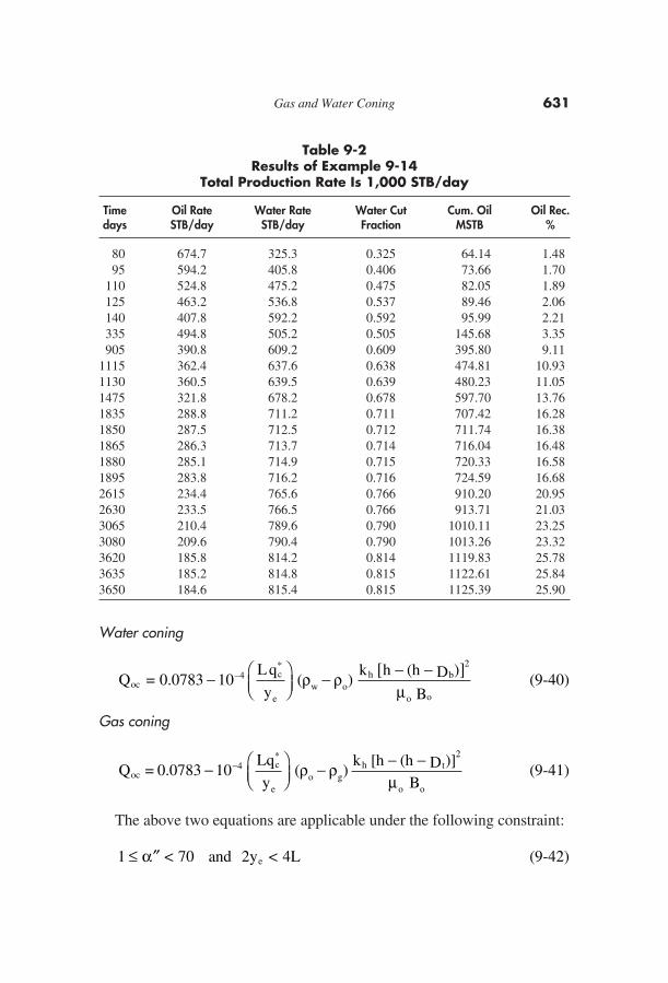
Table 9-2Results of Example 9-14
Total Production Rate Is 1,000 STB/day
Time Oil Rate Water Rate Water Cut Cum. Oil Oil Rec.days STB/day STB/day Fraction MSTB %
80 674.7 325.3 0.325 64.14 1.4895 594.2 405.8 0.406 73.66 1.70
110 524.8 475.2 0.475 82.05 1.89125 463.2 536.8 0.537 89.46 2.06140 407.8 592.2 0.592 95.99 2.21335 494.8 505.2 0.505 145.68 3.35905 390.8 609.2 0.609 395.80 9.11
1115 362.4 637.6 0.638 474.81 10.931130 360.5 639.5 0.639 480.23 11.051475 321.8 678.2 0.678 597.70 13.761835 288.8 711.2 0.711 707.42 16.281850 287.5 712.5 0.712 711.74 16.381865 286.3 713.7 0.714 716.04 16.481880 285.1 714.9 0.715 720.33 16.581895 283.8 716.2 0.716 724.59 16.682615 234.4 765.6 0.766 910.20 20.952630 233.5 766.5 0.766 913.71 21.033065 210.4 789.6 0.790 1010.11 23.253080 209.6 790.4 0.790 1013.26 23.323620 185.8 814.2 0.814 1119.83 25.783635 185.2 814.8 0.815 1122.61 25.843650 184.6 815.4 0.815 1125.39 25.90
Water coning
Gas coning
The above two equations are applicable under the following constraint:
1 < 70 and 2y < 4L (9-42)e≤ ″α
Q = 0.0783Lq
y( )
k [h (h D )]
Boc
c
eo g
2h t
o o
− ⎛⎝⎜
⎞⎠⎟
− − −−10 4*
ρ ρμ
(9-41)
Q = 0.0783Lq
y( )
k h (h D )
Boc
c
ew o
2h b
o o
− ⎛⎝⎜
⎞⎠⎟
− − −[ ]−10 4*
ρ ρμ
(9-40)
Gas and Water Coning 631
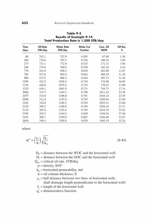
Table 9-3Results of Example 9-14
Total Production Rate Is 1,500 STB/day
Time Oil Rate Water Rate Water Cut Cum. Oil Oil Rec.days STB/day STB/day Fraction MSTB %
80 742.1 757.9 0.505 67.98 1.56260 734.6 765.4 0.510 160.34 3.69275 727.1 772.9 0.515 171.31 3.94290 719.6 780.4 0.520 182.16 4.19770 541.8 958.2 0.639 481.00 11.07785 537.6 962.4 0.642 489.10 11.26800 533.5 966.5 0.644 497.13 11.44
1295 423.5 1076.5 0.718 732.08 16.851310 420.8 1079.2 0.719 738.42 17.001325 418.1 1081.9 0.721 744.71 17.142060 315.7 1184.3 0.790 1011.42 23.282075 314.0 1186.0 0.791 1016.14 23.392090 312.4 1187.6 0.792 1020.84 23.502105 310.8 1189.2 0.793 1025.51 23.602120 309.2 1190.8 0.794 1030.16 23.712135 307.6 1192.4 0.795 1034.79 23.822705 255.5 1244.5 0.830 1194.54 27.503545 200.1 1299.9 0.867 1384.48 31.873650 194.4 1305.6 0.870 1405.19 32.34
where
Db = distance between the WOC and the horizontal wellDt = distance between the GOC and the horizontal well
Qoc = critical oil rate, STB/dayρ = density, lb/ft3
kh = horizontal permeability, mdh = oil column thickness, ft
ye = half distance between two lines of horizontal wells(half drainage length perpendicular to the horizontal well)
L = length of the horizontal wellq*
c = dimensionless function
′′ = ⎛⎝ )α y
h
k
ke v
h
(9-43)
632 Reservoir Engineering Handbook
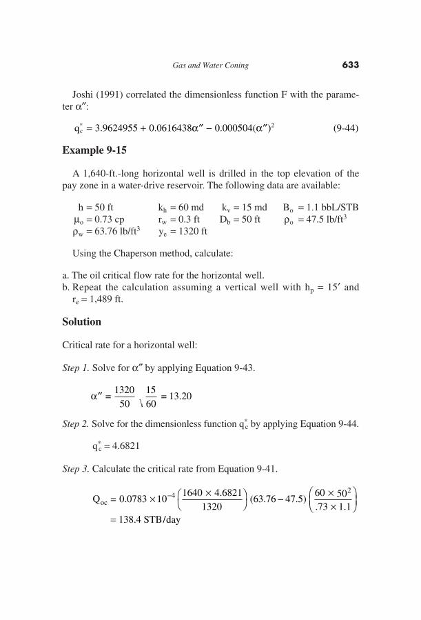
Joshi (1991) correlated the dimensionless function F with the parame-ter α″:
Example 9-15
A 1,640-ft.-long horizontal well is drilled in the top elevation of thepay zone in a water-drive reservoir. The following data are available:
h = 50 ft kh = 60 md kv = 15 md Bo = 1.1 bbL/STBμo = 0.73 cp rw = 0.3 ft Db = 50 ft ρo = 47.5 lb/ft3
ρw = 63.76 lb/ft3 ye = 1320 ft
Using the Chaperson method, calculate:
a. The oil critical flow rate for the horizontal well.b. Repeat the calculation assuming a vertical well with hp = 15′ and
re = 1,489 ft.
Solution
Critical rate for a horizontal well:
Step 1. Solve for α″ by applying Equation 9-43.
Step 2. Solve for the dimensionless function q*c by applying Equation 9-44.
q*c = 4.6821
Step 3. Calculate the critical rate from Equation 9-41.
oc
2Q = 0.0783
1640 4.68211320
(63.76 47.5)60 50.73 1.1
138.4 STB/day
× ×⎛⎝
⎞⎠ − ×
×⎛⎝⎜
⎞⎠⎟
=
−10 4
′′α =1320
501560
= 13.20
qc* . . . ( )= + ′′ − ′′3 9624955 0 0616438 0 000504 2α α (9-44)
Gas and Water Coning 633
Critical rate for a vertical well:
Step 1. Solve for α″ by using Equation 9-19.
α″ = 14.89
Step 2. Solve for q*c by applying Equation 9-18.
q*c = 0.8616
Step 3. Calculate the critical rate for the vertical well from Equation 9-17.
The ratio of the two critical oil rates is
This rate ratio clearly shows the critical rate improvement in the caseof the horizontal well over that of the vertical well.
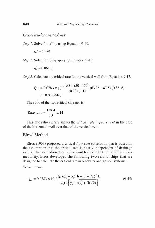
Efros’ Method
Efros (1963) proposed a critical flow rate correlation that is based onthe assumption that the critical rate is nearly independent of drainageradius. The correlation does not account for the effect of the vertical per-meability. Efros developed the following two relationships that aredesigned to calculate the critical rate in oil-water and gas-oil systems:
Water coning
och w o b
o o e e2
Q = 0.0783 k ( ) h (h D ) L
B y + y + (h )×
− − −⎡⎣
⎤−10
3
42
2
ρ ρ
μ
[ ]
/ ⎦⎦(9-45)
Rate ratio =138.4
1014≅
oc4
2Q = 0.0783 10
60 (50 15)(0.73) (1.1)
(63.76 47.5) (0.8616)
= 10 STB/day
× × − −−
634 Reservoir Engineering Handbook
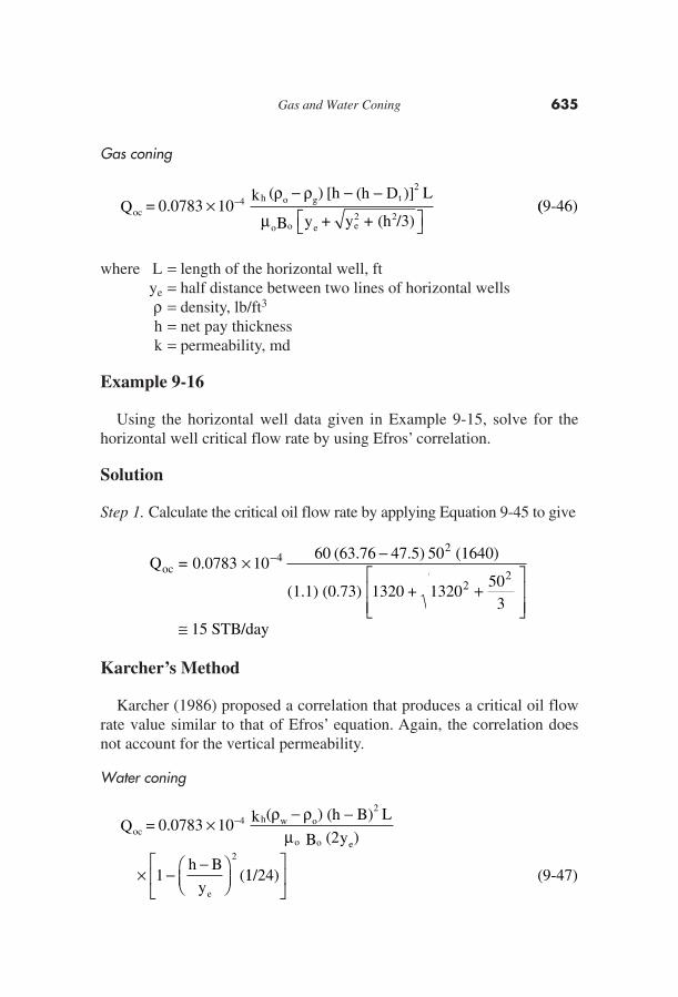
Gas coning
where L = length of the horizontal well, ftye = half distance between two lines of horizontal wellsρ = density, lb/ft3
h = net pay thicknessk = permeability, md
Example 9-16
Using the horizontal well data given in Example 9-15, solve for thehorizontal well critical flow rate by using Efros’ correlation.
Solution
Step 1. Calculate the critical oil flow rate by applying Equation 9-45 to give
Karcher’s Method
Karcher (1986) proposed a correlation that produces a critical oil flowrate value similar to that of Efros’ equation. Again, the correlation doesnot account for the vertical permeability.
Water coning
och w o
2
o o e2
e
Q = 0.0783 k ( ) (h B) L
B (2y )
1h B
y (
×− −
× −−⎛
⎝⎜⎞⎠⎟
−10 4 ρ ρμ
11/24)⎡
⎣⎢
⎤
⎦⎥ (9-47)
ocQ = 0.078360 (63.76 47.5) (1640)
(1.1) (0.73) 1320 +
15 STB/day
× −
+⎡
⎣⎢⎢
⎤
⎦⎥⎥
≅
−1050
132050
3
42
22
oc
h o g2
t
o o e e
Q = 0.0783k ( ) [h (h D )] L
B y + y + (h /3)×
− − −⎡⎣ ⎤⎦
−10 4
2 2
ρ ρ
μ((9-46)
Gas and Water Coning 635
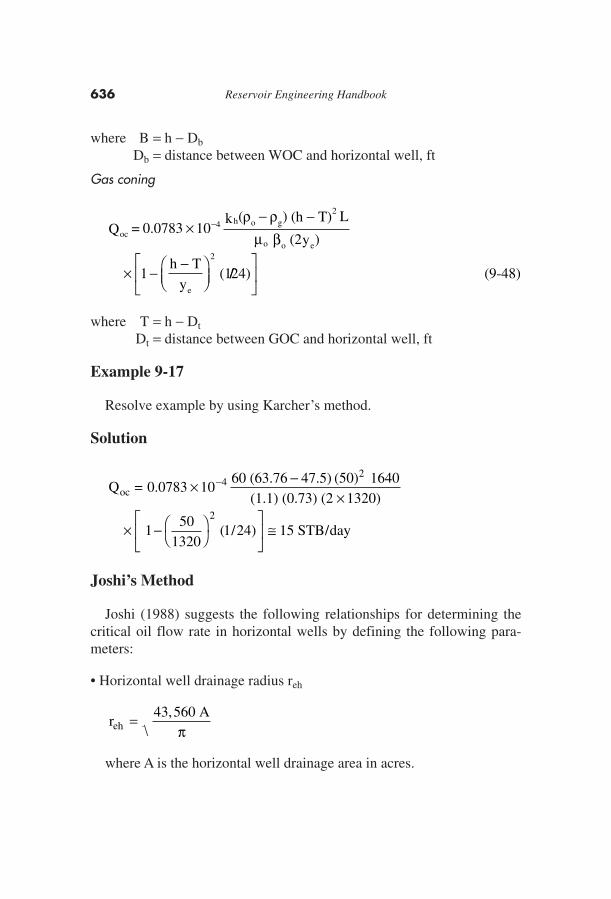
where B = h − Db
Db = distance between WOC and horizontal well, ft
Gas coning
where T = h − Dt
Dt = distance between GOC and horizontal well, ft
Example 9-17
Resolve example by using Karcher’s method.
Solution
Joshi’s Method
Joshi (1988) suggests the following relationships for determining thecritical oil flow rate in horizontal wells by defining the following para-meters:
• Horizontal well drainage radius reh
where A is the horizontal well drainage area in acres.
r43,560 A
eh =π
oc
2
2
Q = 0.078360 (63.76 47.5) (50) 1640
(1.1) (0.73) (2 1320)
150
1320(1/24) 15 STB/day
× −×
× − ⎛⎝
⎞⎠
⎡
⎣⎢
⎤
⎦⎥ ≅
−10 4
oc
h o g2
o o e2
e
Q = 0.0783k ( ) (h T) L
(2y )
1h T
y(1
×− −
× −−⎛
⎝⎜⎞⎠⎟
−10 4ρ ρ
μ β
//24)⎡
⎣⎢
⎤
⎦⎥ (9-48)
636 Reservoir Engineering Handbook
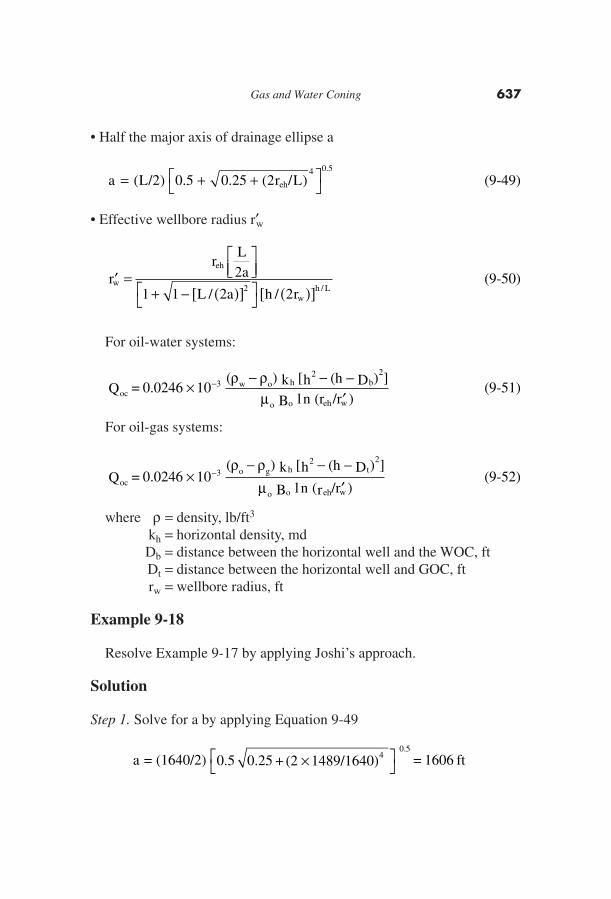
• Half the major axis of drainage ellipse a
• Effective wellbore radius r′w
For oil-water systems:
For oil-gas systems:
where ρ = density, lb/ft3
kh = horizontal density, mdDb = distance between the horizontal well and the WOC, ftDt = distance between the horizontal well and GOC, ftrw = wellbore radius, ft
Example 9-18
Resolve Example 9-17 by applying Joshi’s approach.
Solution
Step 1. Solve for a by applying Equation 9-49
a = (1640/2) 0.5 0.25 + (2 1489/1640) = 1606 ft0.5
4×⎡⎣
⎤⎦
oco g h
2 2t
o o eh w
Q = 0.0246( ) k h (h D )
B l (r /r )×
− − −′
−10 3ρ ρ
μ[ ]
n(9-52)
ocw o h
2 2b
o o eh w
Q = 0.0246( ) k h (h D )
B l (r /r )×
− − −′
−10 3 ρ ρμ
[ ]
n(9-51)
′ =⎡⎣⎢
⎤⎦⎥
+ − ( )[ ]⎡⎣
⎤⎦ ( )[ ]
rr
La
L a h rw
eh
wh L
2
1 1 2 22/ / /(9-50)
a L r Leh= + +⎡⎣
⎤⎦( / ) . . ( / )
.
2 0 5 0 25 24 0 5
(9-49)
Gas and Water Coning 637
Step 2. Calculate r′w from Equation 9-50.
Step 3. Estimate the critical flow rate from Equation 9-51.
HORIZONTAL WELL BREAKTHROUGH TIME
Several authors have proposed mathematical expressions for determin-ing the time to breakthrough in horizontal wells. The following twomethodologies are presented in the following sections:
• The Ozkan-Raghavan method• Papatzacos’ method
The Ozkan-Raghavan Method
Ozkan and Raghavan (1988) proposed a theoretical correlation for cal-culating time to breakthrough in a bottom-water-drive reservoir. Theauthors introduced the following dimensionless parameters:
zWD = dimensionless vertical distance = Db/h (9-54)
where L = well length, ftDb = distance between WOC and horizontal wellH = formation thickness, ftkv = vertical permeability, mdkh = horizontal permeability, md
Ozkan and Raghavan expressed the water breakthrough time by thefollowing equation:
L L h k kD v h= = ( )[ ]dimensionless well length (9-53)/ /2
oc
2 2
Q = 0.0246(63.76 47.5) (60) 50 (50 50)
(0.73) (1.1) l (1489 / 357)= 52 STB/day
× − − −−10 3 [ ]n
′
⎡
⎣⎢
⎤
⎦⎥
+ − ×[ ]⎡⎣⎢
⎤⎦⎥
×r =
1489
1 1 1640 / (2 1606) 50/(2 0.3)= 357 ftw
2 50/1640
16402 1606( )
[ ]
638 Reservoir Engineering Handbook
with the parameter fd as defined by:
fd = φ (1 − Swc − Sor) (9-56)
where tBT = time to breakthrough, dayskv = vertical permeability, mdkh = horizontal permeability, mdφ = porosity, fraction
Swc = connate water saturation, fractionSor = residual oil saturation, fractionQo = oil flow rate, STB/dayEs = sweep efficiency, dimensionless
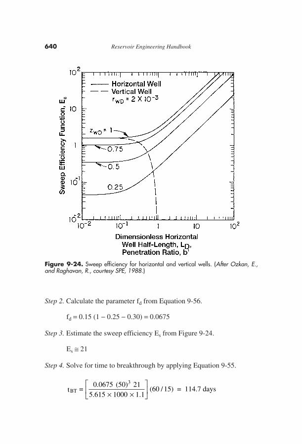
Ozkan and Raghavan graphically correlated the sweep efficiency withthe dimensionless well length LD and dimensionless vertical distanceZWD as shown in Figure 9-24.
Example 9-19
A 1,640-foot-long horizontal well is drilled in a bottom-water-drivereservoir. The following data are available:
h = 50 ft kh = 60 md kv = 15 md Bo = 1.1 bbl/STBμo = 0.73 cp rw = 0.3 ft ρo = 47.5 lb/ft3 ρw = 63.76 lb/ft3
zWD = 1 φ = 15% Swc = 0.25 Sor = 0.3
The well is producing at 1,000 STB/day. Calculate time to break-through.
Solution
Step 1. Solve for LD by using Equation 9-53.
DL = 15 / 60 = 8.216402 50( )
⎡
⎣⎢
⎤
⎦⎥
BTd
3s
o oh vt =
f h E5.615 Q B
(k /k )⎡⎣⎢
⎤⎦⎥
(9-55)
Gas and Water Coning 639
Step 2. Calculate the parameter fd from Equation 9-56.
fd = 0.15 (1 − 0.25 − 0.30) = 0.0675
Step 3. Estimate the sweep efficiency Es from Figure 9-24.
Es ≅ 21
Step 4. Solve for time to breakthrough by applying Equation 9-55.
BT
3
t =0.0675 (50) 21
5.615 1000 1.1(60 / 15) = 114.7 days
× ×⎡
⎣⎢
⎤
⎦⎥
640 Reservoir Engineering Handbook
Figure 9-24. Sweep efficiency for horizontal and vertical wells. (After Ozkan, E.,and Raghavan, R., courtesy SPE, 1988.)
Papatzacos’ Method
Papatzacos et al. (1989) proposed a methodology that is based onsemianalytical solutions for time development of a gas or water cone andsimultaneous gas and water cones in an anisotropic, infinite reservoirwith a horizontal well placed in the oil column.
Water coning
Step 1. Calculate the dimensionless rate qD from the following expression:
where ρ = density, lb/ft3
kv = vertical permeability, mdkh = horizontal permeability, mdh = oil zone thickness, ftL = length of horizontal well
Step 2. Solve for the dimensionless breakthrough time tDBT by applyingthe following relationship:
Step 3. Estimate the time to the water breakthrough tBT by using thewater and oil densities in the following expression:
where tBT = time to water breakthrough as expressed in daysρo = oil density, lb/ft3
ρw = water density, lb/ft3
Gas coning
Step 1. Calculate the dimensionless flow rate qD.
D o o o o g v hq = 20,333.66 B Q / Lh ( ) k kμ ρ ρ−⎡⎣ ⎤⎦ (9-60)
th t
kBT
o DBT
v w o
=−
22 758 528, .
( )
φμρ ρ
(9-59)
DBT DD
D
t = 1 (3q 1) 3q
3q 1− −
−⎡⎣⎢
⎤⎦⎥
ln (9-58)
D o o o w o v hq = 20,333.66 B Q / L h ( ) k kμ ρ ρ−⎡⎣ ⎤⎦ (9-57)
Gas and Water Coning 641
Step 2. Solve for tDBT by applying Equation 9-58.
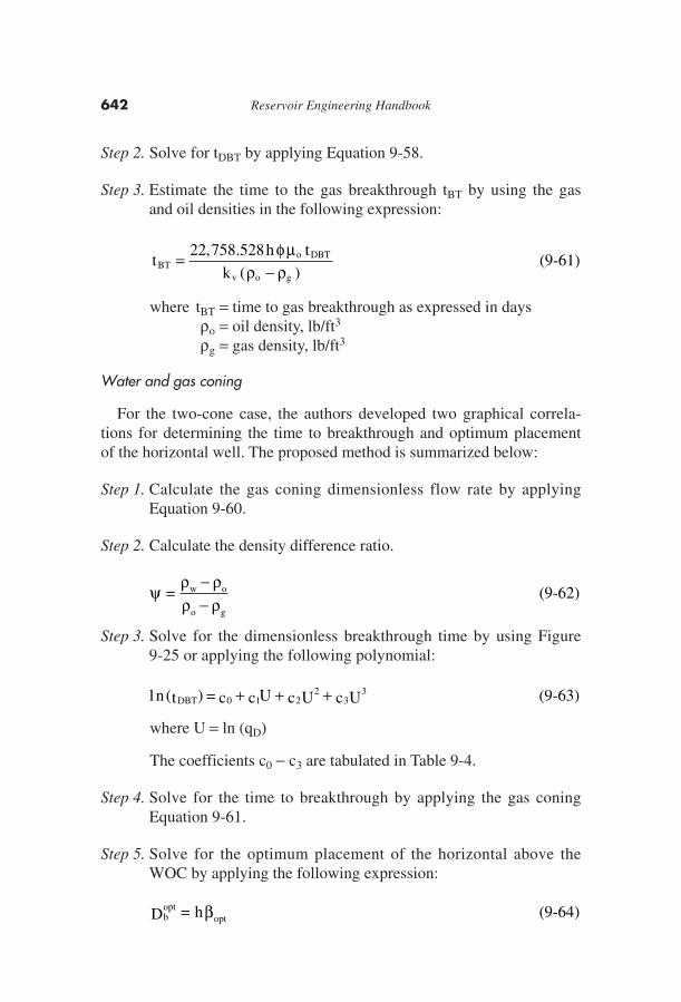
Step 3. Estimate the time to the gas breakthrough tBT by using the gasand oil densities in the following expression:
where tBT = time to gas breakthrough as expressed in daysρo = oil density, lb/ft3
ρg = gas density, lb/ft3
Water and gas coning
For the two-cone case, the authors developed two graphical correla-tions for determining the time to breakthrough and optimum placementof the horizontal well. The proposed method is summarized below:
Step 1. Calculate the gas coning dimensionless flow rate by applyingEquation 9-60.
Step 2. Calculate the density difference ratio.
Step 3. Solve for the dimensionless breakthrough time by using Figure9-25 or applying the following polynomial:
where U = ln (qD)
The coefficients c0 − c3 are tabulated in Table 9-4.
Step 4. Solve for the time to breakthrough by applying the gas coningEquation 9-61.
Step 5. Solve for the optimum placement of the horizontal above theWOC by applying the following expression:
bopt
optD = hβ (9-64)
l (t ) = c c U c U c UDBT 0 1 22
33n + + + (9-63)
ψρ ρρ ρ
= w o
o g
−−
(9-62)
th t
kBT
o DBT
v o g
=−
22 758 528, .
( )
φμρ ρ
(9-61)
642 Reservoir Engineering Handbook
where Dbopt = optimum distance above the WOC, fth = oil thickness, ft
βopt = optimum fractional well placement
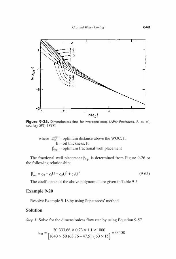
The fractional well placement βopt is determined from Figure 9-26 orthe following relationship:
The coefficients of the above polynomial are given in Table 9-5.
Example 9-20
Resolve Example 9-18 by using Papatzacos’ method.
Solution
Step 1. Solve for the dimensionless flow rate by using Equation 9-57.
Dq =20,333.66 0.73 1.1 1000
1640 50 (63.76 47.5) 60 15= 0.408
× × ×× − ×[ ]
opt 0 1 22
33= c c U c U c Uβ + + + (9-65)
Gas and Water Coning 643
Figure 9-25. Dimensionless time for two-cone case. (After Paptzacos, P. et. al.,courtesy SPE, 1989.)
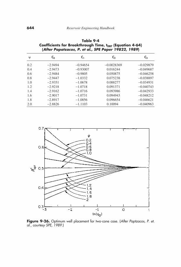
Table 9-4Coefficients for Breakthrough Time, tDBT (Equation 4-64)
(After Papatzacos, P. et al., SPE Paper 19822, 1989)
ψ C0 C1 C2 C3
0.2 −2.9494 −0.94654 −0.0028369 −0.0298790.4 −2.9473 −0.93007 0.016244 −0.0496870.6 −2.9484 −0.9805 0.050875 −0.0462580.8 −2.9447 −1.0332 0.075238 −0.0388971.0 −2.9351 −1.0678 0.088277 −0.0349311.2 −2.9218 −1.0718 0.091371 −0.0407431.4 −2.9162 −1.0716 0.093986 −0.0429331.6 −2.9017 −1.0731 0.094943 −0.0482121.8 −2.8917 −1.0856 0.096654 −0.0466212.0 −2.8826 −1.1103 0.10094 −0.040963
644 Reservoir Engineering Handbook
Figure 9-26. Optimum well placement for two-cone case. (After Paptzacos, P. et.al., courtesy SPE, 1989.)
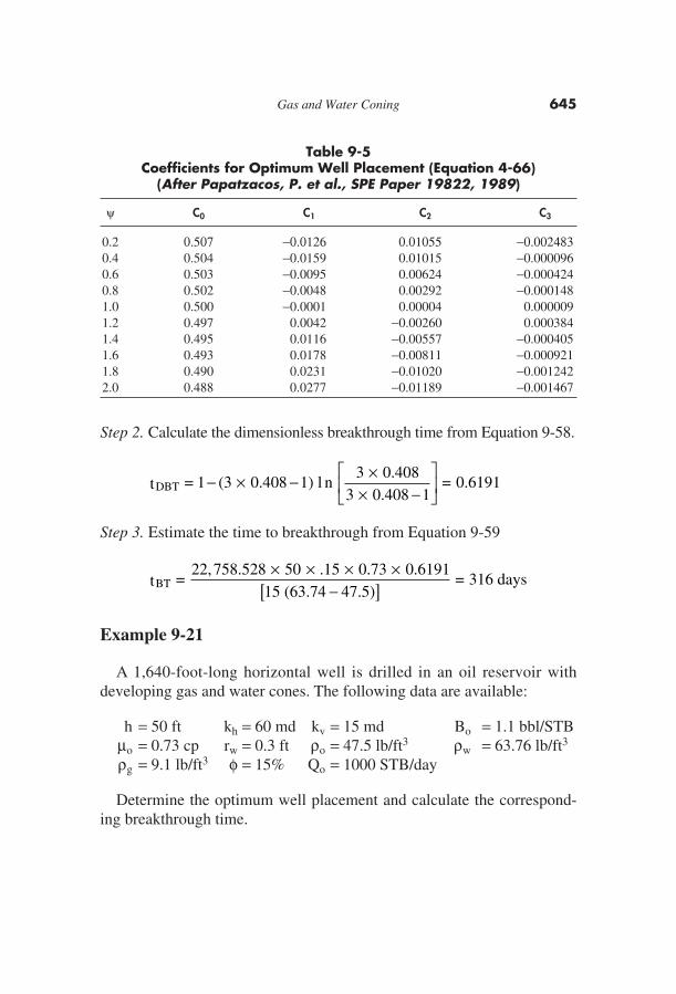
Table 9-5Coefficients for Optimum Well Placement (Equation 4-66)
(After Papatzacos, P. et al., SPE Paper 19822, 1989)
ψ C0 C1 C2 C3
0.2 0.507 −0.0126 0.01055 −0.0024830.4 0.504 −0.0159 0.01015 −0.0000960.6 0.503 −0.0095 0.00624 −0.0004240.8 0.502 −0.0048 0.00292 −0.0001481.0 0.500 −0.0001 0.00004 0.0000091.2 0.497 0.0042 −0.00260 0.0003841.4 0.495 0.0116 −0.00557 −0.0004051.6 0.493 0.0178 −0.00811 −0.0009211.8 0.490 0.0231 −0.01020 −0.0012422.0 0.488 0.0277 −0.01189 −0.001467
Step 2. Calculate the dimensionless breakthrough time from Equation 9-58.
Step 3. Estimate the time to breakthrough from Equation 9-59
Example 9-21
A 1,640-foot-long horizontal well is drilled in an oil reservoir withdeveloping gas and water cones. The following data are available:
h = 50 ft kh = 60 md kv = 15 md Bo = 1.1 bbl/STBμo = 0.73 cp rw = 0.3 ft ρo = 47.5 lb/ft3 ρw = 63.76 lb/ft3
ρg = 9.1 lb/ft3 φ = 15% Qo = 1000 STB/day
Determine the optimum well placement and calculate the correspond-ing breakthrough time.
BTt =22,758.528 50 .15 0.73 0.6191
15 (63.74 47.5)= 316 days
× × × ×−[ ]
DBTt = 1 (3 0.408 1) l3 0.408
3 0.408 1= 0.6191− × − ×
× −⎡
⎣⎢
⎤
⎦⎥n
Gas and Water Coning 645
Solution
Step 1. Calculate the dimensionless flow rate from Equation 9-60.
Step 2. Calculate the density difference ratio from Equation 9-62.
Step 3. Read the fraction well placement βopt from Figure 9-26 by usingthe calculated values of ψ and qD to give:
Bopt ≅ 0.565
Step 4. Calculate the optimum well placement above the WOC fromEquation 9-64.
Dbopt = (0.565) (50) = 28.25 ft
Step 5. From Figure 9-25, for qD = 0.1728 and ψ = 0.4234, find thedimensionless breakthrough time tDBT:
Ln (tDBT) = −.8 (from Figure 9-25)tDBT = 0.449
Step 6. Estimate the time to breakthrough by applying Equation 9-61.
tBT = 22,758.528 × 50 × 0.15 × 0.73 × 0.449/[15 (47.3 − 9.1)]= 97.71 days
PROBLEMS
1. In an oil-water system, the following fluid and rock data are available:
h = 60′ hp = 25′ ρo = 47.5 lb/ft3 ρw = 63.76 lb/ft3
μo = 0.85 cp Bo = 1.2 bbl/STB re = 660 rw = 0.25′ko = k = 90.0 md
ψ =63.76 47.5
47.5 9.1= 0.4234
−−
Dq =20,333.66 0.73 1.1 1000
1640 50 (47.5 9.1) 60 15= 0.1728
× × ×× − ×[ ]
646 Reservoir Engineering Handbook
Calculate the critical oil flow rate, by using the following methods:
• Meyer-Garder• Chierici-Ciucci• Hoyland-Papatzacos-Skjaeveland• Chaney • Chaperson• Schols
2. Given:
Qo = 400 STB/day h = 60 ft hp = 25 ft ρw = 63.76 lb/ft3
ρo = 47.5 lb/ft3 μo = 0.85 cp Bo = 1.2 bbl/STBkv = 9 md kh = 90 md φ = 15% M = 3.5
Calculate the water breakthrough time by using the:
a. Sobocinski-Cornelius methodb. Bournazel-Jeanson correlation
3. The rock, fluid, and the related reservoir properties of a bottom-waterdrive reservoir are given below:
well spacing = 80 acresinitial oil column thickness = 100 ft
hp = 40′ ρo = 48 lb/ft3 ρw = 63 lb/ft3 re = 660′rw = 0.25′ M = 3.0 φ = 14% Sor = 0.25
Swc = 0.25 Bo = 1.2 bbl/STB μo = 2.6 cp μw = 1.00 cpkh = 80 md kv = 16 md
Calculate the water-cut behavior of a vertical well in the reservoirassuming a total production rate of 500, 1,000, and 1,500 STB/day.
4. A 2,000-ft-long horizontal well is drilled in the top elevation of thepay zone in a water-drive reservoir. The following data are available:
h = 50 ft kh = 80 md kv = 25 md Bo = 1.2 bbl/STBμo = 2.70 cp rw = 0.3 ft Db = 50 ft ρo = 48.5 lb/ft3
ρw = 62.50 lb/ft3 ye = 1320 ft
Gas and Water Coning 647
Calculate the critical flow rate by using:
a. Chaperson’s methodb. Efros’ correlationc. Karcher’s equationd. Joshi’s method
5. A 2,000-foot-long horizontal well is producing at 1,500 STB/day. Thefollowing data are available:
h = 60 ft kh = 80 md kv = 15 md Bo = 1.2 bbl/STBμo = 2.70 cp rw = 0.3 ft ρo = 47.5 lb/ft3 ρw = 63.76 lb/ft3
zwD = 1 φ = 15% Swc = 0.25 Sor = 0.25
Calculate the time to breakthrough by using the:
a. Ozkan-Raghavan methodb. Papatzacos’ method
REFERENCES
1. Bournazel, C., and Jeanson, B., “Fast Water Coning Evaluation,” SPE Paper3628 presented at the SPE 46th Annual Fall Meeting, New Orleans, Oct.3–6, 1971.
2. Calhoun, John, Fundamentals of Reservoir Engineering. Norman, OK: TheUniversity of Oklahoma Press, 1960.
3. Chaney, P. E. et al., “How to Perforate Your Well to Prevent Water and GasConing,” OGJ, May 1956, p. 108.
4. Chaperson, I., “Theoretical Study of Coning Toward Horizontal and VerticalWells in Anisotrophic Formations: Subcritical and Critical Rates,” SPE Paper15377, SPE 61st Annual Fall Meeting, New Orleans, LA, Oct. 5–8, 1986.
5. Chierici, G. L., Ciucci, G. M., and Pizzi, G., “A Systematic Study of Gasand Water Coning by Potentiometric Models,” JPT, Aug. 1964, p. 923.
6. Efros, D. A., “Study of Multiphase Flows in Porous Media” (in Russian),Gastoptexizdat, Leningrad, 1963.
7. Hoyland, L. A., Papatzacos, P., and Skjaeveland, S. M., “Critical Rate for WaterConing: Correlation and Analytical Solution,” SPERE, Nov. 1989, p. 495.
648 Reservoir Engineering Handbook
8. Joshi, S. D., “Augmentation of Well Productivity Using Slant and HorizontalWells,” J. of Petroleum Technology, June 1988, pp. 729–739.
9. Joshi, S., Horizontal Well Technology. Tulsa, OK: Pennwell PublishingCompany, 1991.
10. Karcher, B., Giger, F., and Combe, J., “Some Practical Formulas to PredictHorizontal Well Behavior,” SPE Paper 15430, presented at the SPE 61stAnnual Conference, New Orleans, Oct. 5–8, 1986.
11. Kuo, C. T., and Desbrisay, C. L., “A Simplified Method for Water ConingPredictions,” SPE Paper 12067, presented at the Annual SPE Technical Con-ference, San Francisco, Oct. 5–8, 1983.
12. Meyer, H. I., and Garder, A. O., “Mechanics of Two Immiscible Fluids inPorous Media,” J. Applied Phys., Nov. 1954, No. 11, p. 25.
13. Muskat, M., and Wyckoff, R. D., “An Approximate Theory of Water Coningin Oil Production,” Trans. AIME, 1953, pp. 114, 144.
14. Ozkan, E., and Raghavan, R., “Performance of Horizontal Wells Subject toBottom Water Drive,” SPE Paper 18545, presented at the SPE EasternRegional Meeting, Charleston, West Virginia, Nov. 2–4, 1988.
15. Papatzacos, P., Herring, T. U., Martinsen, R., and Skjaeveland, S. M., “ConeBreakthrough Time for Horizontal Wells,” SPE Paper 19822, presented atthe 64th SPE Annual Conference and Exhibition, San Antonio, TX, Oct.8–11, 1989.
16. Pirson, S. J., Oil Reservoir Engineering. Huntington, NY: Robert E. KriegerPublishing Company, 1977.
17. Schols, R. S., “An Empirical Formula for the Critical Oil Production Rate,”Erdoel Erdgas, A., January 1972, Vol. 88, No. 1, pp. 6–11.
18. Slider, H. C., Practical Petroleum Reservoir Engineering Methods. Tulsa,OK: Petroleum Publishing Company, 1976.
19. Sobocinski, D. P., and Cornelius, A. J., “A Correlation for Predicting WaterConing Time,” JPT, May 1965, pp. 594–600.
Gas and Water Coning 649


![pogc.irpogc.ir/Portals/0/maghalat/890901.12.pdf · [7] Russell T.Johns, Larry W.Lake, Rafy Z.Ansari.: "Pridiction of Capillary Fluid Interfaces During Gas or Water Coning in Vertical](https://img.dokumen.tips/doc/110x75/5e0e4ce11f3b21605b15bd20/pogc-7-russell-tjohns-larry-wlake-rafy-zansari-pridiction-of-capillary.jpg)