Embed Size (px)
Citation preview

FEDERAL RESERVE BANK OF DALLAS
EMPLOYER MATCHING AND 401(K)PARTICIPATION: EVIDENCE FROM THE
HEALTH AND RETIREMENT STUDY
Gary V. Engelhardtand
Anil Kumar
Research DepartmentWorking Paper 0601
FEDERAL RESERVE BANK OF DALLAS

Employer Matching and 401(k) Participation:
Evidence from the Health and Retirement Study
Gary V. Engelhardt* Department of Economics and Center for Policy Research
Syracuse University Syracuse, NY 13244
Anil Kumar Research Department
Federal Reserve Bank of Dallas Dallas, TX 75201
Abstract
Employer matching of employee 401(k) contributions can provide a powerful incentive to save for retirement and is a key component in pension-plan design in the United States. Using detailed administrative contribution, earnings, and pension-plan data from the Health and Retirement Study, this analysis formulates a life-cycle-consistent discrete choice regression model of 401(k) participation and estimates the determinants of participation accounting for non-linearities in the household budget set induced by matching. The estimates indicate that an increase in the match rate by 25 cents per dollar of employee contribution raises 401(k) participation by 3.75 to 6 percentage points, and the estimated elasticity of participation with respect to matching ranges from 0.02-0.07. The estimated elasticity of intertemporal substitution is 0.74-0.83. Overall, the analysis reveals that matching is a rather poor instrument with which to raise retirement saving. *Corresponding author. Engelhardt is Associate Professor, Department of Economics, and Senior Research Associate, Center for Policy Research, Syracuse University. Kumar is an economist in the Research Department at the Federal Reserve Bank of Dallas. All research with the restricted-access data from the Health and Retirement Study was performed under agreement in the Center for Policy Research at Syracuse University and the Federal Reserve Bank of Dallas. We thank Dan Black, David Card, Chris Cunningham, Bill Gale, Erik Hurst, Annamaria Lusardi, Brigitte Madrian, Costas Meghir, John Moran, Susann Rohwedder and seminar participants at Syracuse University, University of Chicago, University of Missouri, University of Virginia, Dutch Central Bank, Econometric Society World Congress and Federal Reserve Bank of Dallas for helpful discussions and comments. We are especially grateful to Bob Peticolas and Helena Stolyarova for their efforts in helping us understand the HRS employer-provided pension plan data. The research reported herein was supported (in part) by a grant from the TIAA-CREF Institute and (in part) by the Center for Retirement Research at Boston College pursuant to a grant from the U.S. Social Security Administration funded as part of the Retirement Research Consortium. Various portions of the underlying data construction were funded by the Center for Policy Research at Syracuse University, the Economics Program, National Science Foundation, under Grant No. SES-0078845, National Institute on Aging, under Grant No. 1 R03 AG19895-01, and the U.S. Department of Labor. The opinions and conclusions are solely those of the authors and should not be construed as representing the opinions or policy of the Social Security Administration, or the Federal Reserve Bank of Dallas or the Federal Reserve System , or any agency of the Federal Government, or the Center for Retirement Research at Boston College, TIAA-CREF, the United States Department of Labor, National Science Foundation, National Institute on Aging, or Syracuse University. All errors are our own.

2
I. Introduction
As 401(k)s have come to dominate the private pension landscape in the United
States, researchers and policy makers have given increased attention to the impact of plan
characteristics on retirement-saving decisions.1 One important characteristic is whether
and to what extent the employer matches employee contributions. A typical match might
be 50 cents for each dollar of contribution, up to a maximum percentage of pay, say, 6
percent. Although much of the discussion by the popular press and policy makers
presumes employer matching raises saving, there is actually strikingly little consensus
among researchers. Some studies have found that increases in the match rate raise 401(k)
saving (Papke and Poterba, 1995; Clark and Schieber, 1998; VanDerhei and Copeland,
2001; and Choi, Laibson, Madrian, and Metrick, 2002). Others have found that it is not
the match rate per se that matters, but whether the firm offers a match at all (Even and
Macpherson, 1996; Bassett, Fleming, and Rodrigues, 1998; Papke, 1995; Kusko, Poterba,
and Wilcox, 1998). That is, providing a match raises 401(k) saving, but an increase in
the level of the match rate (conditional on providing a match) does not. Finally, still
other studies (Employee Benefit Research Institute, 1994; Andrews, 1992; Munnell,
Sunden, and Taylor, 1998; and GAO, 1997) have suggested that, conditional on being
eligible for a match, an increase in the match rate lowers 401(k) contributions, which,
when interpreted in the context of a simple two-period model of saving, suggests that the
income effect dominates the substitution effect from the higher rate of return matching
1 This includes work on automatic enrollment (Madrian and Shea, 2001; Choi, Laibson, Madrian, and Metrick, 2002, 2004), investment in company stock (Poterba, 2003; Brown, Liang, and Weisbenner, 2004; Mitchell and Utkus, 2002), portfolio choice and trading in 401(k) plans (Benartzi and Thaler, 2001; Agnew, Balduzzi, and Sunden, 2003).

3
provides.2 Overall, this ambiguity has emerged as an important empirical puzzle in the
literature on saving behavior (Bernheim, 2003).
A central shortcoming in this literature has been the failure to exploit the fact that
employer matching, based either on multiple-match-rate schedules or caps on the
generosity of the match, results in a non-linear household budget set. As has been long
recognized in the study of taxation on labor supply, reduced-form estimates of behavioral
elasticities are biased and inconsistent unless the non-linearity is accounted for explicitly
(Hausman, 1985; Moffitt, 1990; Blundell and MaCurdy, 1999). Indeed, the presence of
budget-set kinks may reconcile some of the findings of previous studies: for example, the
provision of a match may raise 401(k) saving if the substitution effect dominates, but
variation in match rates may not matter if employees are bunched at kinks.
Unlike previous studies, this paper includes a detailed theoretical framework that
models the budget set defined by employer matching and federal tax treatment as twice
continuously differentiable and then uses the first-order conditions from the consumer’s
optimization to derive a life-cycle-consistent discrete choice regression model of 401(k)
participation. As an alternative to the maximum-likelihood piecewise-linear-budget-set
estimation summarized in Hausman (1985)—and the recent, related non-parametric
extensions by Blomquist and Newey (2002)—and the maximum likelihood
differentiable-budget-constraint methodology of MaCurdy, Green, and Paarsch (1990),
this paper employs instrumental-variable techniques that linearize the budget set at the
observed outcome to calculate the price and virtual-income terms and then instruments to
correct for endogeneity, which also has a long history, but a recent example of which is
2 Throughout the paper, “401(k) saving” and “401(k) contributions” are used synonymously as per period flows. In a multi-period model, this would suggest the income effect dominates the substitution and wealth effects (Summers, 1981).

4
Ziliak and Kniesner (1999). To calculate budget-set slopes and virtual income in a
neighborhood around kink points, kernel regression is used to smooth the budget set non-
parametrically.
Empirically, the paper makes four additional contributions. First, to circumvent
difficulties with measurement error in 401(k) contributions and matching incentives that
have plagued previous studies, administrative data from three sources are used:
contributions from W-2 earnings records provided by the Social Security Administration
(SSA) and Internal Revenue Service (IRS); detailed matching formulas from pension
Summary Plan Descriptions (SPD) provided by the employers of Health and Retirement
Study (HRS) respondents; and, a combination of Social-Security-covered-earnings
histories for 1951-1991 and W-2 earnings for 1980-1991, pension SPDs, and pension-
benefit calculators to construct public and private pension entitlements and accruals. The
sample consists of 1,042 individuals in 1991 eligible for 401(k) plans in the HRS.
Second, the analysis includes a calculation of the dollar amount of unused employer
matching contributions due to workers’ failure to contribute at least until the point at
which the employer match is exhausted. Most of this occurs because of non-
participation. For non-participants, the unclaimed employer match represented 3.7
percent of pay. However, even participants left “money on the table” equal to 1 percent
of pay in unclaimed employer match. Based on measures of liquidity constraints used by
others in the literature, reduced-form evidence is not inconsistent with the presence of
liquidity constraints as a potential explanation for this phenomenon. Third, unlike
previous pension studies that have used the employer-provided SPDs in the HRS, which
are available only for a non-random sub-sample of HRS respondents, the estimation

5
corrects for potential sample selection using a set of plausible exclusion restrictions
derived from Internal Revenue Service (IRS) Form 5500 administrative pension-plan
filings. The exclusions have substantial predictive power for determining who is in the
analysis sample. There is statistically significant evidence of selection, and the economic
impact of the selection on the estimates indicates substantial bias. Finally, the variation
in matching incentives is used to estimate a key parameter in public and
macroeconomics, the elasticity of intertemporal substitution, for which there is a large
range of estimates in the previous literature, but econometrically has been identified
poorly because of the lack of independent variation in rates of return. In particular,
employer matching provides large, plausibly exogenous variation in the effective rate of
return that can be used for identification.
The estimates from the life-cycle-consistent discrete choice regression
specifications indicate that the estimated marginal effect of an increase in the employer
match rate by 25 cents per dollar of employee contribution raises 401(k) participation by
3.75 to 6 percentage points. When the estimates are expressed in terms of elasticities, the
results suggest that the impact of the match rate on 401(k) participation is quite inelastic:
the estimated elasticity of 401(k) participation with respect to the match rate ranges from
0.02-0.07. Finally, the estimated elasticity of intertemporal substitution is 0.74-0.83,
comparable to estimates by Attanasio and Weber (1995) and Vissing-Jorgensen (2002),
smaller than those of Gruber (2006), and substantially larger than those by Hall (1988)
and Dynan (1993).
Overall, because of this very inelastic response, the analysis reveals that for
employers and policy makers interested in promoting retirement saving by older workers

6
through greater 401(k) participation, matching is a rather poor policy instrument.
Roughly speaking, the estimated marginal effects in this paper suggest that an increase in
the employer match rate of $1 per $1 of employee contribution would be needed to
achieve the same increase in participation as the implementation of automatic enrollment,
based on the estimates in Madrian and Shea (2001) and Choi, Laibson, Madrian, and
Metrick (2002, 2004). The analysis also suggests that government matching of
voluntary contributions to any type of Social Security personal account would be
relatively ineffective in promoting personal-account contributions (Engelhardt and
Kumar, 2005).
The paper is organized as follows. Section II lays out the theoretical model that
directly motivates the empirical analysis. Section III lays out the econometric framework
and construction of the key variables. Sections IV and V describe the data. Section VI
describes the empirical analysis of the relationship between matching and measures of
liquidity constraints. Section VII discusses the estimation and identification. Section
VIII presents the estimation results. There is a brief conclusion.
II. Theoretical Framework
Previous studies have had two important shortcomings. First, they have not
couched their analyses in formal models of intertemporal choice, even though saving
involves the substitution of resources across time. This means that previous estimates
cannot be interpreted as estimates of life-cycle-consistent determinants of 401(k) saving
necessarily, because the empirical specifications may not have been consistent with
underlying utility maximization. So, while the existing literature has provided quite

7
informative descriptive analyses, it has said little about how 401(k) saving may respond
to prospective changes in employer matching or what the optimal match rate should be to
achieve a saving target. Second, with the exception of Choi, Laibson, Madrian, and
Metrick (2002), Mitchell, Utkus, and Yang (2005), and VanDerhei and Copeland (2001),
previous studies have failed to exploit the fact that multiple-match-rate schedules and
caps on matching induce kinks in the budget set.
By specifying a detailed theoretical framework, this paper represents a stark
departure from the previous literature. In an effort to shorten the exposition, the model is
presented in full in Appendix A and briefly summarized here. It has nine key features:
1) Intratemporal direct utility, );,( zlCU , is derived from leisure, l , with an
associated price, lp , consumption of a composite good, C , with an associated
price, cp , and a vector of demographics, z , and is intratemporally weakly
separable and intertemporally additively separable. 2) The consumer faces a per period probability of survival of ρ , with period T
being the known maximum length of life, and with probability ρ−1 , the
consumer dies and receives the terminal payoff )( TWΦ , the utility of bequests,
which is a function of total wealth, TW .
3) The lifetime is composed of two parts: from period N to Τ , the consumer is retired and no hours of labor are supplied to the market, so leisure equals the time
endowment, and from period 0 to 1-N , the consumer works; the timing of
retirement in period N is endogenous.
4) Total wealth is accumulated in seven forms when working: IRAs, 401(k)s, non-401(k) defined-contribution (DC) pension plans, defined-benefit (DB) pension plans, Social Security, housing equity, and taxable wealth.
5) Retirement-account wealth, defined as the sum of IRA, 401(k), and non-401(k)
DC assets, and taxable wealth can be invested in risky stocks, with stochastic
return sr , and riskless bonds, and, in addition to the optimal asset allocation decision across the different forms of wealth, there is an optimal asset location decision, whereby the consumer must decide which assets to hold in taxable and tax-deferred forms.

8
6) The model specifies in detail non-linearities in the budget set induced by employer matching, the tax treatment of 401(k) and IRA contributions, respectively, IRA withdrawals, including the tax penalty for early withdrawals and minimum-distribution requirements, and the interrelationship between employer matching, 401(k) plan characteristics, and the price of leisure.
7) There are four liquidity constraints: a) non-401(k)-DC, DB and Social Security
wealth are assumed illiquid until retirement and cannot be used as collateral (in accordance with federal law); b) there are constraints on the housing loan-to-value ratio for homeowners which limits the amount of mortgage debt that can be held; c) 401(k) wealth is assumed illiquid until retirement; and d) there is a cash-on-hand constraint, such that total per period full expenditure (also referred to as “full
income” in the two-stage budgeting literature), y , must be less than or equal to
total net cash on hand, where the latter is defined as beginning-of-period liquid taxable wealth and other income on hand, plus the market value of the leisure endowment, less the tax liability, plus any IRA wealth made liquid through a withdrawal, less any tax-deferred saving in the form of contributions to the 401(k) and IRA.
8) In each period t , there are minimum- and maximum-contribution constraints on 401(k)s and IRAs (with multipliers in square brackets), respectively,
0≥VOLtQ , [ 0
tη ] (1)
VOLt
VOLt LQ ≤ , [ L
tη ] (2)
0≥IRAtQ , [ 0
tυ ] (3)
and IRAt
IRAt LQ ≤ , [ L
tυ ] (4)
where VOLQ denotes 401(k) contributions, IRACQ denotes IRA contributions, and VOLL and IRAL are the upper limits on 401(k) and IRA contributions, respectively. IRAL is governed by federal law and depends on marital status and pension
coverage; VOLL is governed by the employer’s plan, but may not exceed the federal statutory maximum.
9) Each period when working, the consumer chooses consumption, leisure, voluntary
401(k) contributions, VOLQ , IRA contributions, IRACQ , IRA withdrawals, the
housing loan-to-value ratio, and the shares of retirement-account and taxable wealth held in risky stocks, respectively. Each period when retired, the consumer chooses consumption, IRA contributions, IRA withdrawals, the housing loan-to-value ratio, and receives eligible pension and Social Security benefits.

9
To summarize, the only forms of “active” saving when working are through
contributions to 401(k), IRA, or taxable assets; adjustments can be made to the mortgage-
debt position as well. However, the primary technology for smoothing resources across
periods when working is through taxable-asset saving, because 401(k) saving is illiquid;
IRA contributions are not necessarily illiquid because of the availability of withdrawals,
but IRA withdrawals may incur a tax penalty; traditional pensions and Social Security are
illiquid; and the extent of mortgage borrowing is limited. This means that the consumer’s
optimization does not imply automatically that all active saving be allocated first to the
tax-preferred asset with the highest net return, because, in the face of uncertainty, the
consumer must balance the desire for a high return with the need for liquidity.
III. First-Order Conditions
As explained in the data section below, consumption and hours are not fully
observed in the HRS, so that, from the perspective of the empirical analysis, it is
desirable to work with the indirect, rather than the direct, utility function. Specifically,
let );,( zp yV be the intratemporal indirect utility function. It takes as arguments the
vector of prices of leisure and consumption, p , full income, y , and the vector of
demographics, z . Following Browning, Deaton, and Irish (1985), let )(* Ttt WV be the
sum of current and future expected utility based on total wealth in period t . The
individual makes all decisions at the beginning of the period, based on the information
set, tΩ , after which, sr is realized, E is the expectations operator conditional on the
information set, and β is the discount rate.

10
The optimization is expressed in terms of two-stage budgeting.3 In the first-
stage, the individual chooses full income, dis-saving through IRA withdrawals, the
mortgage-debt position, and the portfolio allocations to stock of retirement-account and
taxable wealth, and must allocate total “active” saving to three asset categories401(k),
IRA, and taxable wealthto maximize the expected present discounted value of lifetime
indirect utility. In the second stage, optimal full income in each period is allocated
statically between the goods that enter direct utility: consumption and leisure.
The first-order conditions when working for 401(k) contributions, IRA
contributions, and full income can be expressed as
)),1(1(
])1([))]1(1()1([1
*
1401
0
IRAttlyItt
Tt
WtT
tW
tIRAt
tl
yIt
TAt
Vk
tQ
RAttt
Lt
QT
QTRMRE
ζµ
βρβρζηη
−−−
Φ−+⋅−−−+=−++
V (5)
),1(])1([)]1([1
*
1
0tIttT
tW
tTt
WttIt
TAt
RAttt
Lt TTRRE ζµβρβρζυυ −−
Φ−+⋅−−=−++
V (6)
and
tTt
WtT
tW
tTAtttty REyV µβρβρ +
Φ−+=++
])1([);,(1
*
1
Vzp , (7)
respectively. Note that subscripts indicate a partial derivative (other than t , which
denotes time): for example, IT is simply the marginal tax rate; V
QkM 401 is the marginal
employer match rate for an additional dollar of 401(k) contribution; ζ is the fraction of
IRA contributions that is federally tax-deductible; ly
ζ is the change in the fraction of an
IRA contribution that is deductible for an additional dollar of adjusted gross income
3 The necessary condition for two-stage budgeting is that utility be weakly separable (Gorman, 1959). The model assumes strongly intertemporally and weakly intratemporally separable preferences, so that a two-stage budgeting interpretation is valid.

11
(AGI); yV is the marginal utility of full income; tµ is Kuhn-Tucker multiplier on the
cash-on-hand constraint; and RAR and TAR are the weighted average returns on
retirement-account and taxable wealth, respectively.
Even though the typical employer match yields a net return far exceeding that on
other assets, so that it would appear obvious that the individual always would want to
make the maximum possible contribution to the 401(k), equation (5) indicates the role of
liquidity in the 401(k) contribution decision. In particular, there are two ways for this
equation to be satisfied when contributions are less than the plan maximum even when
the match and tax rates are positive, 0401 >V
QkM and 0>IT , respectively, and these occur
when the liquidity constraint binds, 0>µ : (a) the corner solution of no 401(k) saving,
for which the Kuhn-Tucker multipliers on the 401(k) contribution constraints in (1) and
(2) are 00 >η and 0=Lη , respectively; and (b) an interior solution, for which 00 =η
and 0=Lη (i.e., the contribution is positive, but not at the plan maximum), and the
multiplier on the liquidity constraint is large enough that the second term just equals the
first term on the right-hand side of (5). A particularly important example of this latter
case is when the contribution is less than the match cap and the employee leaves “money
on the table” by not contributing up until the point the match is exhausted. Therefore,
even in the presence of an employer match, binding liquidity constraints can explain why
401(k) participation can be less than 100 percent, contributions can be less than the plan
maximum, and employees rationally can leave money on the table. This implication of
the model is examined in Section VII below, in which reduced-form specifications are
estimated to see whether variables used by others in the literature to measure liquidity
constraints can explain who fails to contribute at least until the match is exhausted.

12
IV. Econometric Specification
The major difficulty with the use of (5) as a direct basis for estimating the impact
of employer matching on 401(k) participation is that most of elements on the right-hand
side are not fully observed in survey data: who is liquidity constrained, µ ; expectations,
E; the sum of future expected utility, *V ; bequest motives, Φ ; and the discount rate, β ,
for example. To overcome this, define the following tax/match prices, tItIRAt Tp ζ−≡ 1 ,
Vk
tQ
mt Mp 4011+≡ , and )1(1401 IRA
tt
ly
Itk
t QTp ζ−−≡ , and then combine (5)-(7) to solve out
for the unobserved elements to yield
tmtttytt pyVp υη ∆+⋅∆=∆ );,( zp , (8)
where 0t
Ltt ηηη −≡∆ , 0
tLtt υυυ −≡∆ , and kIRAm pppp 401−≡∆ .4
Equation (8) motivates the functional form for estimation. In particular,
following Blundell, Browning, and Meghir (1994), let the indirect utility function take
the following Box-Cox form
Ψ⋅
−
=)](ln[
)(1
)();,(
p
zpzp
b
a
y
yVλ
λ
, (9)
where when 0=λ ,
)](ln[
)](ln[)ln()();,(
p
pzzp
b
ayyV
−⋅Ψ= , (10)
which is a member of the class of the PIGLOG indirect utility functions (Muellbauer,
1976), that has been used extensively in the literature on consumption. The factor Ψ is a
4 These three prices are not for goods that enter the intratemporal direct utility function and, therefore, are not in the price vector p that is an argument in the indirect utility function.

13
utility scaling factor that is a function of the exogenous demographic characteristics. In
(9), b is homogeneous of degree zero and modeled as a Cobb-Douglas price aggregator
∏=k
kkpbγ
)(p , (11)
across the k goods that enter the direct utility function, where 0=∑k
kγ . Because there
are only two goods that enter direct utility, leisure )1( =k and consumption )2( =k ,
respectively, this implies 12 γγ −= , so that (11) can be re-written as
kbγω=)(p , (12)
where cl pp /≡ω is the real relative price of leisure. In addition, a is homogeneous of
degree one and defined as
221 )][ln()ln()](ln[)](ln[ ωωω aaaa +==p . (14)
The marginal indirect utility of full income, yV , is
λλ −−
Ψ= )(
)](ln[
)( 1p
p
zay
bVy . (15)
The scaling factor Ψ is modeled as
∑=Ψm
mimi z ,)( ψz , (16)
where z is an 1×m vector that includes a constant. The second term on the right-hand
side of (8) is zero when IRA saving is at an interior solution, positive when constrained
by the upper IRA limit, and negative when at the lower IRA limit (of zero). Finally, let
)( 0DDp
IRALm −≡κ , (17)

14
where IRA
LD is a dummy variable that is one if IRA contributions, which are measured in
the HRS, are at the upper limit and zero otherwise, and 0D is a dummy variable that is
one if IRA contributions are zero and zero otherwise.
Because, as will be illustrated in the discussion of the descriptive statistics, there
is a very small percentage of workers in the sample whose contributions equal the 401(k)
plan maximum, we consider just the participation decision in the empirical analysis, so
that η∆ collapses to 0η− , and (8), (15), (16), and (17) combine to yield the following
discrete choice econometric model
jitijtijt
m ijt
ijt
ijtijt
ijt
mimijt ua
y
y
pzδ +++
∆=− ∑ αxκδ
ωωη
λ
2,10
)()ln( (18)
and
,0 0 if 0
0 0 if 1
0*
0*
<−⇔==
=−⇔>=
ijtVOLijt
VOLijt
ijtVOLijt
VOLijt
QD
QD
η
η (19)
where 11 / γψδ mm ≡ , i and j index individuals and 401(k) plans, respectively, and u is
the error term. If an increase in the employer match raises participation, then the null
hypothesis 0215141312110 ======= δδδδδδδ should be rejected, and the
estimated marginal effect and elasticity of participation to the match rate should be
positive.
In the empirical analysis, z includes a constant, the worker’s education (in years),
age, and dummy variables for whether the worker was married, white, and female,
respectively. These demographic characteristics enter parsimoniously and allow the
impact of employer matching to be heterogeneous across demographic groups. The last
term on the right-hand side of (18) includes x , a vector that contains a constant and

15
exogenous employer and employment characteristics. These are additional factors,
explained in section VIII below, that fall outside of the scope of the theoretical
framework, but may affect contributions. In the baseline specifications, x is limited to a
constant; additional specifications allow the employer and employment characteristics to
enter x .
V. Data
Previous research primarily has used nationally representative, individual-level
survey data, such as the Current Population Studies (CPS) and Surveys of Consumer
Finances (SCF), which are plagued by two important sources of measurement error.
First, even though the researcher must know the entire match schedule for a plan to
account for the individual’s full opportunity set, as well as whether the match is
discretionary or through profit-sharing, the typical survey respondent has great difficulty
in accurately conveying even relatively simple pension provisions to interviewers, no less
detailed matching schedules.5 Second, self-reported contribution data also suffer from
substantial reporting error. In addition, as the theoretical framework showed, the data
required to model saving are quite extensive: contributions, components of household
(including spousal) income, assets, debts, demographics, marginal tax rates, spousal
pension coverage, and expected entitlements from Social Security and traditional
pensions, which require lifetime and job earnings histories, respectively. Previous studies
have not had all of these data.
5 See Mitchell (1988), Starr-McCluer and Sunden (1999), Johnson, Sambamoorthi, and Crystal (2000), Gustman and Steinmeier (1999), Rohwedder (2003a, 2003b), and Engelhardt (2001) for evidence on measurement error in pension data.

16
In this paper, these problems are overcome by using remarkably detailed data
from the first wave of the HRS, a nationally representative random sample of 51-61 year
olds and their spouses (regardless of age). The first wave asked detailed questions about
wealth (including IRA and taxable assets), demographics, and spousal characteristics in
1992. The survey also asked detailed questions about household income, tax
information, and IRA contributions, but, as is true in many household surveys, these
questions were for the previous calendar year, 1991. So, for the purposes of the empirical
analysis, periods t and 1+t refer to 1991 and 1992, respectively.
Questions on employment were asked for the job (if any) held at the time of the
interview, as well as previous jobs. A unique feature of these data is that the HRS used
the job rosters from the household interviews and collected Summary Plan Descriptions
(SPDs), which are legal descriptions of pensions written in plain English, from employers
of HRS respondents for all current and previous jobs in which the respondent was
covered by a pension. These descriptions help to sidestep the problems with
measurement error outlined above, and, instead, measure the exact incentives to
contribute by using the employer matching formulas given in the SPD.6 Specifically, the
job in which the respondent was employed in 1991 was identified and then SPDs
associated with that job that had dates of adoption after 1991 were excluded. In addition,
the date of last amendment and dates for changes in plan provisions indicated in the text
of the SPD were used to exclude plans that were in existence in 1991 but whose features
changed between 1991 and the time the SPD was collected.
6 The data appendix explains why self-reported pension information was not used and some other data limitations in the HRS.

17
The HRS also asked in the first wave the respondents’ permission to link their
survey responses to administrative earnings data from SSA and IRS. These
administrative data include Social Security covered-earnings histories from 1951-1991
and W-2 earnings records for jobs held from 1980-1991, and were made available for use
under a restricted-access confidential data agreement. They are the basis for two critical
measures in the analysis dataset. First, the W-2 data provide administrative data on
earnings and 401(k) contributions for 1991. Unlike the contributions data used in
previous studies, these data are not subject to measurement error, as they are the
employer’s official report to the government on annual earnings and elective deferrals.
Second, when combined, the W-2 earnings histories, Social Security covered-earnings
histories and self-reported earnings histories, allowed for the construction of complete
earnings histories from 1951-1991 for each member of our sample. When used with
Social Security and pension-benefit calculators, which are described in Appendix A,
these data allowed for the calculation of the public and private pension wealth, accruals
and changes in accruals, for 1991 and 1992, respectively.
Overall, when all of the sources are combined, the data are a comprehensive
description of the household’s financial situation and exact pension incentives in 1991
and 1992 to estimate the parameters in the empirical specification in (51)-(52) and a
significantly richer data source than previous studies. Specifically, the sample consists
of 1,042 HRS individuals eligible to contribute to a 401(k) in 1991.
VI. Descriptive Statistics

18
Many plans limit the amount of the match. These caps are usually expressed as a
percent of pay in the SPD, but also can be a percent of contributions, and even a fixed-
dollar amount. Table 1 shows the distribution of matching caps in the analysis sample,
expressed as a percent of annual pay. About 19 percent of these plans had caps on
employer matching that were less than four percent of pay. The median cap was 6
percent of pay, but 15 percent of plans had higher caps. Plans also vary according to the
match rate. Table 2 shows the distribution of “first-dollar” match rates in the analysis
sample. Columns 1 and 2 indicate that these match rates were clustered at 25, 50, and
100 percent, where the median match rate was 50 percent. However, 27 percent of the
plans offered matches of 100 percent, and three plans offered match rates of 200 percent.
Descriptive statistics for selected variables used in the empirical analysis are
shown in Table 3. Column 1 shows sample means for the full sample, with the standard
deviation in parentheses, and the median in square brackets. Overall, the sample consists
of mostly white, married individuals in their mid-50s, with some college education and
relatively few children at home. Only 56.4 percent of the sample actively participated
(defined as having made a positive contribution) in 1991. The sample mean 401(k)
contribution in calendar year 1991 was $1,377, but among contributors, the average
contribution was $2,446 (shown in column 4). Only 3 percent of the sample made the
maximum contribution. A comparison of contributions between those without and with
employer matching in columns 2 and 3, respectively, indicates that individuals with
matching contributed just over $400 more on average than those without matching (i.e.,
$1,640-$1,232=$408). The difference in the median contributions between these two
groups was $800.

19
A comparison of columns 2 and 3 in Table 3 also indicates that plans with
employer matching differ along other dimensions that may make saving attractive. For
example, if there is an employer match, the individual is much more likely to be able to
borrow against the plan balance, direct the investment of plan balances, less likely to
have another traditional pension plan, more likely to have the plan annual contribution
limit lower than the federal limit, and more likely to be allowed to make after-tax
contributions to the plan.
VII. Explaining Unused Employer Matching Contributions
Because the typical employer match yields a return far exceeding that on
alternative investments, 401(k) participation would be predicted to be 100 percent if all
individuals were fully informed, financially rational, with access to perfect capital
markets and no transactions costs. In addition, at a minimum, all participants would be
predicted to maximize total compensation and contribute up to the point at which the
employer match was exhausted and then engage in a set of borrowing and lending
arrangements to achieve the desired level of consumption and leisure.7 Yet in Table 3,
401(k) participation is 56.4 percent among all sample individuals, and only 54 percent
among those offered a match. This suggests that individuals left “money on the table” by
not capturing the total potential employer match.
Column 1 of Table 4 shows the total potential employer match in the sample for
individuals eligible for a match. The mean potential match was $1,249, or 3.8 percent of
annual pay. The average employer match that went unused because contributions were
7 A similar argument would imply that all individuals would be predicted to contribute up to the plan limit, and engage in a set of borrowing and lending arrangements to achieve the desired consumption and leisure, and thus exploit the tax arbitrage from deferral to minimize the lifetime tax liability.

20
not made up to the level of the match cap was $550, or 1.9 percent of pay. Naturally,
non-participants accounted for most of this, with the unused match equal to 3.7 percent of
pay (column 3). Even more striking, though, is that among participants the average
unused employer match represented 1 percent of pay (column 2).8
As described in the theoretical framework, one possible explanation for this is that
individuals were liquidity constrained. To explore this, ad hoc reduced-form models
were estimated measuring whether and to what extent the 401(k) contribution was less
than the cap on the employer match as a function of a set of explanatory variables that
measure (to varying degrees) the ability to borrow, which have been used by others in the
previous literature on liquidity constraints, but none of which measure such constraints
definitively: demographics (white, age, married, and years of education); dummy
variables for whether the household has no capital income; has access to borrowing
against home equity through a home equity line of credit, conditional on being a home
owner; has experienced financial distress in the past due to unanticipated medical
expenses and unemployment, respectively; and has access to informal private support
from friends and family if under financial distress.9
The results are shown in Table 5 for the sub-sample of individuals offered a
match. Sub-sample means are shown in column 1. Column 2 shows estimates from a
probit model in which the dependent variable is one if the individual contributed below
8 Choi et al. (2005) and Mitchell, Utkus, and Yang (2005) have similar findings using various sets of company data. 9 This section of the paper includes the results of ad hoc reduced-form models of the impact of liquidity constraints on “money on the table” only to provide some evidence in support of (or at least not inconsistent with) the mechanism in the theoretical framework that would explain individuals’ failure to fully exploit the employer matching and tax-deferral in 401(k)s—namely, liquidity constraints. In particular, measures of liquidity constraints used by others in the literature are used here simply for comparative purposes. There are at least two other explanations for the presence of unused employer matching contributions, imperfect information and present-biased preferences, both of which we discuss in the appendix.

21
the employer match cap (including a zero contribution) and zero otherwise. Individuals
who were more educated or with a home equity line of credit were statistically
significantly less likely to have contributed below that match cap, whereas those
individuals who had financial distress from unanticipated medical expenses or no capital
income were statistically significantly more likely to have contributed below that match
cap. Columns 3 and 4 show estimates for Tobit models of the dollar amount and the
percentage of pay of the unused employer match, respectively, and the results are
qualitatively similar. These results are not inconsistent with the theoretical result that
constrained borrowing is a plausible explanation for why workers fail to capture the total
potential employer match.
VIII. Estimation and Identification
The estimation employs an instrumental-variable technique that linearizes the
budget set at the observed outcome to calculate the price and virtual income terms and
then instrument to correct for endogeneity. In particular, for all observed 401(k)-
contribution outcomes in the dataset, the tax and match prices, IRAp , m
p , and kp
401 , the
net wage, ω , and full income, y , must be calculated in order to construct )ln(/ ωyp∆
and κ in (18). Because budget-set slopes are not defined at kink points, a variant of the
method of MaCurdy, Green, and Paarsch (1990) was used to calculate IRAp , m
p , and
kp
401 for each individual in the sample. Specifically, the matching formulas in the
SPDs, tax-rate information from NBER’s TAXSIM calculator, and detailed household
financial and demographic characteristics were used to lay out the budget set in detail,
then the kinks in the budget set were smoothed non-parametrically using kernel

22
regression of the implicit (negative) tax rate from the employer matching and tax subsidy
to contributions on AGI over the federal legally allowable range of 401(k) contributions
of 0 to $9500 using a second-order Gaussian kernel, 2/2
)2/1()( zezK
−= π , with
bandwidth chosen by Silverman’s rule of thumb, 5/1/9.0 nmh = , where
)349.1/,varmin( xx iqrm = and iqrx is the inter-quartile range.10 This regression was
done on an individual-by-individual basis, so that the smoothing is individual-budget-set
specific, and the estimates allow for budget-set slopes to be measured for those
individuals located at kink points.
Full income, y , can be expressed as
itIRAWit
IRACit
VOLit
oit
lit
TAitit TQQQyLwAy −+−−++∆≡ , (20)
and includes the market value of the leisure endowment. Under two-stage budgeting, the
capital income and net (dis-)saving terms embodied in A∆ are sufficient statistics for the
past and the expectations of future variables (Blundell and Macurdy, 1999). Because of
the non-linear structure of matching and marginal tax rates, the tax and match prices,
IRAp , m
p , and kp
401 , change depending upon the budget-set segment (either because the
marginal match rate or tax rate changes), and, hence, the taxes-paid measure, T , which,
in turn, incorporates the dollar amount of the implicit tax liability from the employer-
matching and tax subsidies, will change depending upon the budget-set segment as well.
Therefore, full income is actually measured as “virtual” full income, vy , according to the
respective budget segment, where vT denotes the associated implicit tax liability, which
10 See Appendix A for details.

23
is calculated by numerically integrating the estimated kernel-smoothed implicit tax
function described above.
Unfortunately, the explanatory variables in (18) have components based on choice
variables. Therefore, the instrument set, Z , includes the vector of demographics, z , and
three additional variables, FCitZ 1− , IRAzmz pp ⋅ , and kzp 401 : the first is a dummy variable if
the household was in poor financial condition in 1990, and the second and the third are
based on “first-dollar” match and marginal tax rates for a synthetic taxpayer in 1989.
There are two primary sources of variation in the instruments. First, mzp varies by plan,
j . That is, it is assumed that the variation in matching schedules across plans is
exogenous. Second, IRAzp and kzp401 vary across synthetic individuals because the tax
function is non-linear in income and marital status. Appendix B gives a detailed
description of the construction of the instruments and discusses the sources of
identification in detail.
A final issue is that the sample is likely non-random because it is based on
individuals for whom the HRS was able to obtain an employer-provided SPD for the
401(k) plan. Although previous pension studies using the HRS employer-provided SPDs
have not corrected for selection because of the lack of plausible exclusion restrictions,
two exclusion restrictions based on IRS Form 5500 data were used to estimate the model
using a number of methods to correct for selection. The first exclusion is the incidence of
pension-plan outsourcing by Census region, employment-size category, one-digit SIC
code, and union status (union plan vs. non-union plan) cell in 1992, where outsourcing
means the plan was administered by an entity other than the employer. The intuition is
that the HRS is less likely to obtain an SPD from the employer if (on average in its cell)

24
plan administration is outsourced, because more than one contact is needed (first the
employer, then the plan administrator) to receive the SPD. The second exclusion is the
incidence of pension-plan consolidation due to mergers and acquisitions by cell from
1988-1992. The intuition is that the HRS is less likely either to obtain an SPD from the
employer or match it to the employee if (on average in its cell) there has been a lot of
plan consolidation, because plan names and detail are often changed upon consolidation.
Finally, two other variables based on HRS data were used as exclusions in the selection
equations: dummies for whether the individual left the job because the business closed or
was laid off, respectively. These help to measure whether the employer possibly was in
financial difficulty at severance, which, if that resulted in a business failure, would have
made it more difficult for the HRS to have obtained an SPD. The construction of the
exclusions and the selection equation are discussed in detail in Appendix B.
IX. Estimation Results
The parameters in (18) are estimated in the baseline specification, in which the
vector x in is limited to a constant, by maximum likelihood, where ),0(~ 2σNu , under
the parameter restriction that 0=λ . As shown in (10), this implies a PIGLOG indirect
utility function, which has been used extensively in the consumption literature. From a
practical perspective, this parameter restriction is useful, because when 0=λ , the
regression index in (18) becomes linear in parameters 2,δ1δ , and α , which simplifies
computations substantially.11
11 Appendix C provides estimates from ad hoc reduced-form models similar to those used in the previous literature for those readers who wish to compare the results in Table 6 with previous methods.

25
Panel A of Table 6 presents parameter estimates with standard errors in
parentheses.12 Panel B lists the set of additional explanatory variables in the models.
Column 1 shows the parameter estimates for the baseline specification without
instrumenting. The marginal effect for a one unit change in the match rate represents an
increase of one dollar of match per dollar of employee contribution and is shown in Panel
C. The estimated marginal effect of an increase in the match rate by one dollar is an
increase in participation of 0.0091 or nine-tenths of a percentage point, which is
economically extremely small and statistically different than zero, based on the p-value
for the test of the null hypothesis of no impact of employer matching shown in panel A.
The estimated marginal effect for virtual full income is negative, consistent with
consumption and leisure as normal goods, statistically significantly different than zero,
but, again, the economic magnitude of the income elasticity is very small.
Column 2 gives the instrumental-variable estimates. In panel B, an increase in the
match rate of one dollar increases contributions by an estimated 27 percentage points and
is statistically different than zero. This estimate is substantially larger than the one in
column 1 without instrumenting, which indicates substantial downward bias in the
estimated match effect from endogeneity. In column 2, the income effect is negative and
indicates that an increase of one unit in virtual full income, which represents an increase
of $100,000, results in an estimated reduction in the probability of participation of eight
percentage points. The income effect, as well as the impact of the net wage and the
marginal tax rate, are all significant at less than the 0.0001 level of significance for all of
the specifications in Table 6.
12 The standard errors account for the presence of the estimated selection-correction and the use of instrumental variables.

26
To get a better sense of the economic magnitude of these marginal effects, Panel
D shows the estimated elasticity of participation with respect to the employer match rate,
evaluated at the sample means. In column 2, the estimated elasticity is 0.07: if the
employer match were raised from twenty-five to fifty cents (i.e., doubled), participation
would rise by seven percent (not percentage points).13 Thus, 401(k) participation
appears to be quite inelastic with respect to the employer match. The estimated income
elasticity is 10.0− ; the estimated net wage elasticity is 04.0− ; and the estimated
elasticity with respect to the marginal tax rate is 0.04, so that 401(k) participation also is
very inelastic with respect to the tax price.
Panel A also shows the parameter estimates on the exclusion restrictions in the
selection model.14 The p-value for the test of the null hypothesis that the exclusions
jointly do not explain who has a matched SPD, though not shown in the table, is less than
0.01, which indicates the exclusions have predictive power for who is in the sample. In
particular, greater plan outsourcing, consolidation, business closure and layoffs
significantly decrease the likelihood of having a matched SPD. The parameter estimate
on the selection term in the participation equation is negative, and, based on the
associated standard error, the null hypothesis of no selection bias can be rejected at the 3
percent level of significance. This is evidence of selection: high savers are less likely to
have an employer-provided SPD in the HRS, consistent with the reduced-form analysis
of Gustman and Steinmeier (1999). To gauge whether this selection is economically
important, column 3 shows the IV results without selection correction. The estimated
participation elasticity with respect to the match rate in Panel E is now 0.195, which is
13 The estimated elasticities are very similar when based on individual characteristics. 14 Parameter estimates for the full selection model are available upon request.

27
more than double the selection-corrected elasticity of 0.07 in column 2. This indicates
that the bias from estimating the determinants of 401(k) participation on the selected
sample of the respondents in the HRS who have matched SPDs has a substantial effect on
the economic magnitude of the employer match estimates.
Robustness Checks and Extensions
There are two practical concerns in the estimation that fall outside of the scope of
the theoretical framework. First, firms may offer employer matching contributions as a
way to try to avoid failing federal pension non-discrimination rules because they have
low-saving employees (McGill, et al., 1996). This would tend to bias downward the
estimated match elasticity. Second, firms that match may adopt other plan features to
stimulate employee saving (e.g., allow for borrowing against plan balances, self-directed
investment, offer after-tax saving options, offer retirement seminars, etc.) or offer
different fringe benefit packages that might affect saving behavior than firms that do not
match. This would tend to bias upward the estimated match elasticity.
The reduced-form relationship between employer match rates and these factors
using the HRS data was examined in a companion paper, Engelhardt and Kumar (2004a).
As described there, the non-discrimination rules are set up so that employers with a
greater proportion of workers with earnings large enough to be deemed “highly-
compensated employees” under federal law face greater pressure to meet non-
discrimination rules if they offer a 401(k). In particular, a variable that measured the
share of workers with earnings above the federal threshold for the definition of a “highly-
compensated” employee under federal non-discrimination regulations in the respondent’s

28
Census-region-by-employment-size-category-by-one-digit-SIC-code-by-union-status cell
in 1989 was constructed from the March CPS. This measure was then weighted by the
difference in combined federal and state marginal tax rates on earnings for the median
highly- and non-highly-compensated workers in the cell to reflect the value a highly-
compensated worker would put on a dollar of tax-deferred salary through a 401(k)
relative to that for a non-highly-compensated worker. This tax-difference-weighted share
was used as a measure of the non-discrimination “pressure” faced by the typical
employer in the respondent’s cell in a reduced-form model of the determinants of match
rates in the HRS data.
The estimation results in Engelhardt and Kumar (2004a) showed that the measure
of pressure and other plan characteristics were highly significant. For example, the
greater the pressure (tax-difference-weighted share) the more likely the respondent’s plan
offered a match and the higher the match rate. Also, plans that allowed borrowing, self-
directed investment, had other traditional features, had limits less than the federal limit,
and after-tax saving options had significantly higher first-dollar employer match rates, as
was suggested in the comparison of unconditional means in Table 3 of the current
paper.15
With this in mind, two groups of additional explanatory variables were included
in the vector x in (18) for the specification in Table 6: 1) fringe benefits offered: dummy
variables for whether the firm offered long-term disability and group term life insurance,
respectively, as well as the number of health insurance plans, number of retiree health
15 Another potential concern is that high-saving individuals, such as those with long horizons, might sort to firms that offer employer matching contributions (Ippolito, 1997). This would tend to bias upward the estimated elasticity of voluntary contributions to matching. However, the estimation results in Engelhardt and Kumar (2004a) showed no correlation of the employer match rate with measures of the demographics and horizon and offered no support for endogenous sorting.

29
insurance plans, weeks paid vacation, and days of sick pay; 2) other plan characteristics:
dummy variables for whether the 401(k) allowed borrowing, hardship withdrawals, self-
directed investment, had an after-tax saving option, a 401(k) contribution limit less than
the federal limit, respectively, whether the firm offered other traditional pensions, and the
measure of non-discrimination “pressure” described above.
Column 4 Table 6 shows the estimation results for this specification. In
particular, in panel B, the estimated marginal effect of a one-dollar increase in the match
rate is an increase in participation of 0.09, or nine percentage points. The estimated
match rate elasticity, Panel E, is 0.02, compared to 0.07 in column 2, so that the addition
of the fringe benefit and other plan characteristics has an important impact on the results.
The estimated marginal effects for income, net wage, and the marginal tax rate also
decline relative to those in the baseline specifications in column 2.
In column 5, a third set of explanatory variables was added to x in (18): 3)
additional employment characteristics: dummy variables for both the worker and spouse
for whether the firm offered a retirement seminar, discussed retirement with co-workers,
whether responsible for the pay and promotion of others, the number of supervisees,
spousal pension coverage, as well as controls for firm size, Census division, and union
status. These additional employment characteristics were interacted with the fringe
benefit and plan characteristics described above to allow a more flexible functional form
for xα in (18). The estimated marginal effects for the match rate, income, net wage,
and marginal tax rate are shown in column 5, respectively, are similar to those in the
baseline specifications in columns 2 and 4, respectively. The estimated elasticity of
participation to the match rate rises to 0.05 in Panel E.

30
Finally, to allow for a significantly more flexible functional form for xα in (18),
in column 6, occupation dummies were added; the fringe benefit, plan, and other
employment characteristics were interacted with occupation; and, the other plan
characteristics were interacted with the fringe benefit variables. Hence, the specification
in column 6 is essentially fully interactive in the elements of x . The estimated elasticity
of participation to the match rate rises to 0.06 (column 6, Panel E).
As noted in section III, the demographic characteristics enter (18) parsimoniously,
in a manner that allows the impact of employer matching to be heterogeneous across
demographic groups. Across columns in Table 6, the demographic group for which the
employer match consistently appears to have statistically significant differential effects
on contributions is the relatively highly educated. To highlight any differences in
responsiveness across groups, Table 7 shows the estimated marginal effect and
elasticities for the employer match rate by sex and education group for the richest
specification, shown in column 6 of Table 6. In columns 1 and 2 of Table 7, an increase
in the match rate of one dollar increases participation of males and females by an
estimated 22.6 and 17.5 percentage points, respectively. However, the estimated 95%
confidence intervals around these estimates overlap substantially and these effects are not
statistically different from each other.16 In columns 3-7, the marginal effect rises sharply
by education group. When measured in terms of the elasticities, there is little difference
across education group, primarily because the participation rate that enters the
denominator for the elasticity formula also rises sharply with education, causing the
elasticities to be relatively flat across groups.
16 Given the length of Tables 6-8, the confidence intervals for the marginal effects and elasticities have been omitted for the sake of brevity in exposition, but are available upon request.

31
Estimating the Elasticity of Intertemporal Substitution
One potential drawback of the estimates in Tables 6 is that they were based on the
parameter restriction that 0=λ . Because the elasticity of intertemporal substitution
(EIS) is defined as yyy yVV /)(− , the EIS for the more general Box-Cox utility function in
(9) is )1/(1)( λ−− .17 For the PIGLOG, 0=λ , so that the EIS is implicitly constrained to
1. Although well-known papers by Hall (1988) and Dynan (1993) suggest point
estimates of the EIS for the United States that are close to zero, a more recent literature
finds substantially larger point estimates: Attanasio and Weber (1995), from 6.0 to 7.0 ;
Vissing-Jorgenson (2002), 3.0 to 4.0 for stockholders and 8.0 to 1 for bondholders;
Gruber (2005), from 5.1 to 2.2 . Many of the confidence intervals around these estimates
include 1. This suggests that, in principle, an assumed EIS of 1 might not be a
completely unreasonable assumption.
In practice, to test this assumption, the parameters in (18) were estimated for the
specifications in columns 2 and 4-6 in Table 6 by non-linear maximum likelihood
(NLML), allowing for λ to be unconstrained, as in the Box-Cox formulation of utility in
(9); the associated estimate of λ , the EIS, marginal effects, and participation elasticities
are reported in columns 1-4 of Table 8, respectively. The NLML estimation yielded
estimates of λ that range from 20.0− to 35.0− and are significantly different than zero,
which represents PIGLOG utility, at the 6 percent level of significance or less, depending
upon the specification. Although from a purely statistical point of view, these results
17 Even though the EIS is technically negative in this formulation (Browning, 1985), estimates of the EIS will be presented in absolute value so as to more easily facilitate comparisons for the reader with well-known estimates of the EIS from the consumption Euler-equation literature, where, in the Euler equation, the EIS is expressed as a positive number.
32
reject the PIGLOG, the estimated marginal effects and elasticities of participation with
respect to the match rate differ little between the PIGLOG and the more general Box-Cox
utility functions for the richest specification, shown in column 6 of Table 6 for the
PIGLOG and column 4 of Table 8 for the Box-Cox. For example, the marginal effect of
a $1 increase in the match rate is 0.1977 based on the PIGLOG, while for the more
general Box-Cox, the marginal effect is 0.1499. In addition, the participation elasticity
with respect to the match rate is 0.0561 for the PIGLOG versus 0.0448 for the Box-Cox.
Therefore, in terms of the economic magnitude of the match rate estimates, there is little
difference between the two utility function specifications. Based on the NLML estimates
in Table 8, the implied EIS ranges from 0.74-0.83. This is consistent with the estimates
by Attanasio and Weber (1995) and Vissing-Jorgensen (2002), smaller than those in
Gruber (2006), and substantially larger than those by Hall (1988) and Dynan (1993).
One seeming puzzle that arises from the results in Table 8 is that while the EIS
estimates suggest that older workers are reasonably responsive to changes in the
intertemporal price of full income in their intertemporal allocation decisions, the marginal
effects and participation elasticities suggest these workers are quite unresponsive to the
employer match rate in their 401(k) saving decision. This can be reconciled by noting
that the relevant marginal rate of return governing the intertemporal allocation decision
can be thought of as a weighted average of the marginal returns for each of the
components of full income, where the weights depend on each component’s share of full
income. The sample mean of full income is $150,000, and the federal maximum 401(k)
contribution in 1991 was $9500. Because maximum 401(k) saving only represented
roughly 6 percent of full income (i.e., 063.0150000/9500 = ), the elasticity of 401(k)

33
saving to the 401(k) marginal return (which includes the employer match), would
expected to be about 6 percent of the EIS or less, which would imply a match elasticity of
0.04-0.06 for an EIS of 0.7-1. These are the same order of magnitude as the match
elasticities estimated in Tables 6 and 8, which means the empirical results are internally
coherent.
X. Summary and Implications
Previous studies have produced a puzzling array of estimates of the impact of
employer matching on 401(k) saving. This probably stemmed from the use of less than
ideal data and, more importantly, the failure to incorporate into estimation match-induced
kinks in the budget set. Overall in this analysis, based on the life-cycle consistent
specification derived, the estimated elasticity of 401(k) participation with respect to the
match rate ranged from 0.02-0.07, and, hence, participation was quite inelastic with
respect to employer matching.
There are two potential implications and two obvious limitations of these
findings. First, a number of commonly-advocated reforms to Social Security call for the
introduction of voluntary private accounts, to which individuals could choose to
contribute additional funds toward Social Security. Under some proposals, the federal
government would match those contributions as an incentive. In designing such a
system, it would be instrumental for policy makers to know how individual contributions
would respond to the government match. Clearly, much could be learned in this context
from the experience of employer matching for 401(k)s. This is examined in more detail
in a companion paper (Engelhardt and Kumar, 2005). Second, a number of prominent

34
companies have reduced or eliminated matching contributions recently due to declining
profits. Although it remains to be seen if this is a long-term trend, understanding the
impact of matching is critical to understanding the impact of these changes on retirement
income security for a workforce increasingly dependent on 401(k) plans for retirement.
The fact that the estimated response of contributions to the employer match was quite
inelastic suggests that overall 401(k) activity at these firms might not be greatly affected
by these changes in matching. An important caveat is that focus was on older workers,
for whom the very detailed data for this type of study were available; whether the
estimates apply to younger workers is an open question. Finally, this study has nothing
to say about the broader question of to what extent 401(k) saving constitutes new private
saving, a point of substantial debate in the literature.

35
References
Agnew, Julie, Pierluigi Balduzzi, and Annika Sunden, “Portfolio Choice and Trading in a Large 401(k) Plan,” American Economic Review 93:1 (2003): 193-215. Andrews, Emily S., “The Growth and Distribution of 401(k) Plans,” in Trends in
Pensions 1992, John A. Turner and Daniel J. Beller, eds. (Washington, DC: U.S. Department of Labor) 1992, pp. 149-176. Attanasio, Orazio P., and Guglielmo Weber, “Is Consumption Growth Consistent with Intertemporal Optimization? Evidence from the Consumer Expenditure Survey,” Journal
of Political Economy 103:6 (1995): 1121-1157. Barksy, Robert B., F. Thomas Juster, Miles S. Kimball, and Matthew D. Shapiro, “Preference Parameters and Behavioral Heterogeneity: An Experimental Approach in the Health and Retirement Study,” Quarterly Journal of Economics 112:2 (1998): 537-580. Bassett, William F., Michael J. Fleming, and Anthony P. Rodrigues, “How Workers Use 401(k) Plans: The Participation, Contribution, and Withdrawal Decisions,'” National Tax
Journal 51:2 (1998): 263-289. Bayer, Patrick J., B. Douglas Bernheim, and John Karl Scholz, “The Effects of Financial Education in the Workplace: Evidence from a Survey of Employers,” NBER Working Paper No. 5655, 1996. Benartzi, Shlomo, and Richard H. Thaler, “Naïve Diversification Strategies in Defined Contribution Saving Plans,” American Economic Review 91:1 (2001): 79-98. Benartzi, Shlomo, and Richard H. Thaler, “Save More Tomorrow: Using Behaviorial Economics to Increase Employee Saving,” Journal of Political Economy 112: S1 (2004): S164-S187. Bernheim, B. Douglas, “Taxation and Saving,” in Alan J. Auerbach and Martin Feldstein, eds., Handbook of Public Economics, Volume 3 (Amsterdam: North Holland), 2003, pp. 1173-1249. Bernheim, B. Douglas, and Daniel M. Garrett, “The Effects of Financial Education in the Workplace: Evidence from a Survey of Households,” Journal of Public Economics 87 (2003): 1487-1519. Bernheim, B. Douglas, Daniel M. Garrett, and Dean M. Maki, “Education and Saving: The Long-Term Effects of High School Curriculum Mandates,” Journal of Public
Economics 80 (2001): 435-465. Blomquist, Soren, and Whitney Newey, “Nonparametric Estimation with Nonlinear Budget Sets,” Econometrica 70 (2002): 2455-2480.

36
Blundell, Richard, Martin Browning, and Costas Meghir, “Consumer Demand and the Life-Cycle Allocation of Expenditures,” Review of Economic Studies 61:1 (1994): 57-80. Blundell, Richard, and Thomas MaCurdy, “Labor Supply: A Review of Alternative Approaches,” in Orley Ashenfelter and David Card, eds., Handbook of Labor Economics,
Volume 3A, (Amsterdam: North Holland), 1999, pp. 1559-1695. Blundell, Richard W., and James L. Powell, “Endogeneity in Semiparametric Binary Response Models,” Review of Economic Studies 71:3 (2004a): 655-680. Blundell, Richard, and James L. Powell, “Censored Regression Quantiles with Endogeneous Regressors,” Mimeo., University College London, 2004b. Brown, Jeffrey R., Nellie Liang, and Scott Weisbenner, “401(k) Matching Contributions in Company Stock: Costs and Benefits for Firms and Workers,” NBER Working Paper No. 10419, 2004. Browning, Martin, Angus Deaton, and Margaret Irish, “A Profitable Approach to Labor Supply and Commodity Demands over the Life-Cycle,” Econometrica 55:3 (1985): 503-544. Buchinsky, M., “Changes in the U.S. Wage Structure 1963-1987: Application of Quantile Regression,” Econometrica, 62(2) (1994): 405-459. Burtless, Gary, and Jerry Hausman, “The Effect of Taxation on Labor Supply: Evaluating the Gary Income Maintenance Experiment,” Journal of Political Economy 86 (1978): 1103-1130. Campbell, John Y., and Joao Cocco, “Household Risk Management and Optimal Mortgage Choice,” Quarterly Journal of Economics 118:4 (2003): 1449-1494. Carroll, Christopher D., “The Buffer-Stock Theory of Saving: Some Macroeconomic Evidence,” Brookings Papers on Economic Activity 2 (1992): 61-156. Choi, James J., David Laibson, Brigitte C. Madrian, “Plan Design and 401(k) Savings Outcomes,” National Tax Journal, forthcoming, 2004. Choi, James J., David Laibson, Brigitte C. Madrian, and Andrew Metrick, “Defined Contribution Pensions: Plan Rules, Participant Decisions, and the Path of Least Resistance,” in James M. Poterba, ed., Tax Policy and the Economy, Vol. 16 (Cambridge, MA: MIT Press), 2002. Choi, James J., David Laibson, Brigitte C. Madrian, and Andrew Metrick, “Optimal Defaults,” American Economic Review 93:2 (2003a): 180-185.

37
Choi, James J., David Laibson, Brigitte C. Madrian, and Andrew Metrick, “Passive Decisions and Potent Defaults,” NBER Working Paper No. 9917, 2003b. Choi, James J., David Laibson, Brigitte C. Madrian, and Andrew Metrick, “Optimal Defaults and Active Decisions: Theory and Evidence from 401(k) Saving,” Harvard University Working Paper, 2003c. Choi, James J., David Laibson, Brigitte C. Madrian, and Andrew Metrick, “For Better or Worse: Default Effects and 401(k) Savings Behavior,” in David A. Wise, ed., Perspectives in the Economics of Aging (Chicago: University of Chicago Press), forthcoming, 2004. Clark, Robert L. and Sylvester J. Schieber, “Factors Affecting Participation Rates and Contribution Levels in 401(k) Plans,” in Living with Defined Contribution Pensions:
Remaking Responsibility for Retirement, Olivia S. Mitchell and Sylvester J. Schieber, eds. (Philadelphia: University of Pennsylvania Press), 1998, pp. 69-97. Coile, Courtney, and Jonathan Gruber, “Social Security and Retirement,” NBER Working Paper No. 7830, 2000. Cunningham, Christopher R., and Gary V. Engelhardt, “Federal Tax Policy, Employer Matching, and 401(k) Saving: Evidence from HRS W-2 Records,” National Tax Journal, 55 (2002): 617-645. Dammon, Robert M., Chester S. Spatt, and Harold H. Zhang, “Optimal Consumption and Investment with Capital Gains Taxes,” Review of Financial Studies 14:3 (2001): 583-616. Dammon, Robert M., Chester S. Spatt, and Harold H. Zhang, “Optimal Asset Location and Allocation with Taxable and Tax-Deferred Investing,” Journal of Finance 59:3 (2004): 999-1037. Das, Mitali, Whitney K. Newey, and Francis Vella, “Nonparametric Estimation of Sample Selection Models,” Review of Economic Studies 70:1 (2003): 33-63. Deaton, Angus, “Saving and Liquidity Constraints,” Econometrica 59:5 (1991), 1221-1248. Diamond, Peter, and Botond Koszegi, “Quasi-hyperbolic Discounting and Retirement,” Journal of Public Economics 87 (2003): 1839-1872. Duflo, Esther, and Emmanuel Saez, “Participation and Investment Decisions in a Retirement Plan: The Influence of Colleagues’ Choices,” Journal of Public Economics 85 (2002): 121-148.

38
Duflo, Esther, and Emmanuel Saez, “The Role of Information and Social Interactions in Retirement Plan Decisions,” Quarterly Journal of Economics 118:3 (2003): 815-842. Dynan, Karen E., “How Prudent Are Consumers?” Journal of Political Economy 101:6 (1993): 1104-1113. Elmendorf, Douglas W., “The Effect of Interest-Rate Changes on Household Saving and Consumption: A Survey,” Federal Reserve Board Finance and Economics Discussion Series Paper No. 1996-27, 1996. Employee Benefit Research Institute, Salary Reduction Plans and Individual Saving for
Retirement, Issue Brief No. 155 (Washington, DC: Employee Benefit Research Institute), 1994. Engelhardt, Gary V., “Consumption, Down Payments, and Liquidity Constraints,” Journal of Money, Credit, and Banking, 28:2 (May) 1996: 255-271.
Engelhardt, Gary V., “Have 401(k)s Raised Household Saving? Evidence from the Health and Retirement Study,” Mimeo., Syracuse University, 2001. Engelhardt, Gary V., “Pre-Retirement Lump-Sum Pension Distributions and Retirement Income Security: Evidence from the Health and Retirement Study,” National Tax Journal
55:4 (December) 2002: 665-686. Engelhardt, Gary V., “Reasons for Job Change and the Disposition of Pre-Retirement Lump-Sum Pension Distributions” Economics Letters 81:3 (December) 2003a: 333-339. Engelhardt, Gary V., “Nominal Loss Aversion, Housing Equity Constraints, and Household Mobility: Evidence from the United States,” Journal of Urban Economics 53:1 (January) 2003b: 171-195. Engelhardt, Gary V., “Defined Contribution Pension Plans and the Measurement of Retirement Wealth: Implications for Studies of Pension Knowledge, Saving, and the Timing of Retirement,” Mimeo, Syracuse University, 2004. Engelhardt, Gary V. and Anil Kumar, “Understanding the Impact of Employer Matching on 401(k) Saving,” TIAA-CREF Institute Research Dialogue No. 76, 2003. Engelhardt, Gary V. and Anil Kumar, “Sorting and 401(k) Employer Matching,” Syracuse University Mimeo., 2004a. Engelhardt, Gary V. and Anil Kumar, “Social Security Personal-Account Participation with Government Matching,” Journal of Pension Economics and Finance 4:2 (2005): 155-179.

39
Engen, Eric M., William G. Gale, and John Karl Scholz, “The Illusory Effects of Saving Incentives on Saving,” Journal of Economic Perspectives 10:4 (1996): 113-137. Even, William E., and David A. Macpherson, “Factors Influencing Employee Participation in 401(k) Plans,” Mimeo, Miami University (Ohio), 1996. Feenberg, Daniel, and Elisabeth Coutts, “An Introduction to the TAXSIM Model,” Journal of Policy Analysis and Management 12 (1) (Winter) (1993): 189-194. General Accounting Office, “401(k) Pension Plans: Loan Provisions Enhance Participation But May Affect Income Security for Some,” Report GAO/HEHS-98-5, 1997. Gomes, Francisco, Alexander Michaelides, Valery Polkovnichenko, “Portfolio Choice and Wealth Accumulation with Taxable and Tax-Deferred Accounts,” Mimeo., London Business School, 2004. Gorman, W.M., “Separable Utility and Aggregation,” Econometrica 27:3 (1959): 469-481. Gourinchas, Pierre-Olivier, and Jonathan A. Parker, “Consumption over the Life-Cycle,” Econometrica 70:1 (2002): 47-89. Gruber, Jonathan, “A Tax-Based Estimate of the Elasticity of Intertemporal Substitution,” NBER Working Paper No. 11945, 2006. Gustman, Alan L., and Thomas L. Steinmeier, “What People Don’t Know About Pensions and Social Security: An Analysis Using Linked Data from the Health and Retirement Study,” NBER Working Paper No. 7368, 1999. Gustman, Alan L., Olivia S. Mitchell, Andrew A. Samwick, and Thomas L. Steinmeier, “Pension and Social Security Wealth in the Health and Retirement Study,” in Wealth,
Work, and Health: Innovations in Measurement in the Social Sciences, James Smith and Robert Willis, eds. (Ann Arbor: University of Michigan Press) 1999, pp. 150-208. Hall, Robert, “Intertemporal Substitution in Consumption,” Journal of Political Economy 96 (1988): 339-57. Hausman, Jerry A., “The Econometrics of Nonlinear Budget Sets,” Econometrica (November) 53 (1985), 1255-1282. Honore, Bo E., and Luojia Hu, “Estimation of Cross-Section and Panel Data Censored Regression Models with Endogeneity,” Journal of Econometrics 122:2 (2004): 293-316. Honore, Bo E., and James L. Powell, “Pairwise Difference Estimation of Nonlinear Models,” Princeton University, Mimeo., 2002.

40
Hubbard, R. Glenn, and Jonathan S. Skinner, “Assessing the Effectiveness of Saving Incentives,” Journal of Economic Perspectives 10:4 (1996): 73-90. Ibbotson Associates, “Stocks, Bonds, Bills and Inflation, 2003 Yearbook (Chicago: Ibbotson Associates), 2003. Ippolito, Richard A. Pension Plans and Employee Performance, Chicago: University of Chicago Press, 1997. Jappelli, Tullio, Jorn-Steffen Pischke, and Nicholas S. Souleles, “Testing for Liquidity Constraints in Euler Equations with Complementary Data Sources,” Review of
Economics and Statistics 80:2 (1998): 251-262. Johnson, Richard W., Usha Sambamoorthi, and Stephen Crystal. "Pension Wealth at Midlife: Comparing Self-Reports with Provider Data." Review of Income and Wealth 46(1) (2000): 59-83. Joulfaian, David, and David Richardson, “Who Takes Advantage of Tax-Deferred Savings Programs? Evidence from Federal Income Tax Data,” National Tax Journal 54 (2001): 669-688. Kusko, Andrea, James M. Poterba, and David Wilcox, “Employee Decisions With Respect to 401(k) Plans,” in Living with Defined Contribution Pensions: Remaking
Responsibility for Retirement, Olivia Mitchell and Sylvester Schieber, eds. (Philadelphia: University of Pennsylvania Press) 1998, pp. 98-112. Laibson, David, “Golden Eggs and Hyperbolic Discounting,” Quarterly Journal of
Economics 112 (1997): 443-477. Laibson, David, Andrea Repetto, and J. Tobacman, “Self-Control and Retirement Savings,” Brookings Papers on Economic Activity 1 (1998): 91-196. MaCurdy, Thomas E., David Green, and Harry Paarsch, “Assessing Empirical Approaches for Analyzing Taxes and Labor Supply,” Journal of Human Resources 25 (Summer 1990): 415–90. Madrian, Brigitte C., and Dennis F. Shea, “The Power of Suggestion: Inertia in 401(k) Participation and Savings Behavior,” Quarterly Journal of Economics 116 (2001): 1149-87. McGill, Dan M., Kyle N. Brown, John J. Haley, and Sylvester J. Schieber, Fundamentals
of Private Pensions, Seventh Edition (Philadelphia: University of Pennsylvania Press), 1996.

41
Mitchell, Olivia S., “Worker Knowledge of Pension Provisions,” Journal of Labor
Economics 6 (1988): 21-39. Mitchell, Olivia, Jan Olson, and Thomas Steinmeier, “Construction of the Earnings and Benefits File (EBF) for Use with the Health and Retirement Survey,” HRS/AHEAD Documentation Report No. DR-001, Institute for Social Research, University of Michigan, 1996. Mitchell, Olivia S., and Stephen P. Utkus, “The Role of Company Stock in Defined Contribution Plans,” NBER Working Paper No. 9250, 2002. Moffitt, Robert A., “The Econometrics of Piecewise-Linear Budget Constraints,” Journal
of Business and Economic Statistics 4 (1986): 317-328. Moffitt, Robert A., “The Econometrics of Kinked Budget Constraints,” Journal of
Economic Perspectives 4 (1990): 119-139. Munnell, Alicia H., Annika Sunden, and Catherine Taylor, “What Determines 401(k) Participation and Contributions?” Mimeo., Boston College, 2001. Newey, Whitney K., “Linear Instrumental Variable Estimation of Limited Dependent Variable Models with Endogenous Explanatory Variables,” Journal of Econometrics 32 (1986): 127–141. Newey, Whitney K., “Specification Tests for Distributional Assumptions in the Tobit Model,” Journal of Econometrics 34 (1987a): 125–145. Newey, Whitney K., “Efficient Estimation of Limited Dependent Variable Models with Endogenous Explanatory Variables,” Journal of Econometrics 36 (1987b): 231–250. O’Donoghue, Ted, and Matthew Rabin. “Incentives for Procrastinators.” Quarterly
Journal of Economics 114:3 (1999a): 769-816. O’Donoghue, Ted, and Matthew Rabin. “Doing It Now or Later.” American Economic
Review 89:1 (1999b): 103-124. Papke, Leslie E., “Participation in and Contributions to 401(k) Pension Plans: Evidence from Plan Data,” Journal of Human Resources 30:2 (1995): 311-325. Papke, Leslie E., Poterba, James M, “Survey Evidence on Employer Match Rates and Employee Saving Behavior in 401(k) Plans”, Economics Letters 49, 313-317, 1995.
Poterba, James M., “Employer Stock and 401(k) Plans,” American Economic Review, 93:2 (2003): 398-404.

42
Poterba, James M., Clemens Sialm, and John B. Shoven, “Asset Location for Retirement Savers,” in William G. Gale, John B. Shoven, and Mark J. Warshawsky, eds. Private
Pensions and Public Policies. Washington: Brookings Institution, 2001. Poterba, James M., Steven F. Venti, and David A. Wise, “How Retirement Saving Programs Increase Saving,” Journal of Economic Perspectives 10:4 (1996): 91-112. Rohwedder, Susann, “Empirical Validation of HRS Pension Wealth Measures,” Mimeo., Rand Corporation, (2003a). Rohwedder, Susann, “Measuring Pension Wealth in the HRS: Employer and Self-Reports,” Mimeo., Rand Corporation, 2003b. Shoven, John B., “The Location and Allocation of Assets in Pension and Conventional Savings Accounts,” NBER Working Paper No. 7007, 1999. Shoven, John B., and Clemens Sialm, “Long Run Asset Allocation for Retirement Savings,” Journal of Private Portfolio Management 1 (2) (1998): 13-26.
Shoven, John B., and Clemens Sialm, “Asset Location in Tax-Deferred and Conventional Savings Accounts,” Journal of Public Economics 88 (2003): 23-38. Staiger, Douglas, and James H. Stock, “Instrumental Variables Regression with Weak Instruments,” Econometrica 65:3 (1997): 557-586. Starr-McCluer, Martha, and Annika Sunden, “Workers’ Knowledge of Their Pension Coverage: A Reevaluation,” Mimeo., Federal Reserve Board of Governors, 1999. Summers, Lawrence H., “Capital Taxation and Accumulation in a Life Cycle Model,” American Economic Review 71 (1981): 533-544. U.S. Department of Labor, 1993 Private Pension Plan Bulletin (Washington, DC: U.S. Department of Labor), 1995. U.S. Government Printing Office, 2004 Economic Report of the President (Washington, DC: U.S. Government Printing Office), 2004. Vanderhei, Jack, and Craig Copeland, “A Behavioral Model for Predicting Employee Contributions to 401(k) Plans: Preliminary Results,” North American Actuarial Journal 5:1 (2001): 80-94. Vella, Francis, “Simple Tests for Sample Selection Bias in Censored and Discrete Choice Models,” Journal of Applied Econometrics 7:4 (1992): 412-421. Vissing-Jorgensen, Annette, “Limited Asset Market Participation and the Elasticity of Intertemporal Substitution,” Journal of Political Economy 110:4 (2002): 825-853.

43
Ziliak, James, and Thomas Kniesner, “Estimating Life Cycle Labor Supply Tax Effects,” Journal of Political Economy 107 (April 1999): 326-359.

44
Appendix A
This appendix lays out the theoretical model in more detail. Additional detail can be provided upon request. This appendix is intended to be supplemental and, given its length, not published.
Previous studies have had two important shortcomings. First, they have not
couched their analyses in formal models of intertemporal choice, even though saving involves the substitution of resources across time. This means that previous estimates cannot be interpreted as estimates of life-cycle-consistent determinants of 401(k) saving necessarily, because the empirical specifications may not have been consistent with underlying utility maximization. So, while the existing literature has provided quite informative descriptive analyses, it has said little about how 401(k) saving may respond to prospective changes in employer matching or what the optimal match rate should be to achieve a saving target. Second, with the exception of Choi, Laibson, Madrian, and Metrick (2002) and VanDerhei and Copeland (2001), previous studies have failed to exploit the fact that multiple-match-rate schedules and caps on matching induce kinks in the budget set.18
To illustrate the kink, Figure 1 shows budget sets with and without matching in a simple two-period model of consumption (without borrowing) typically used in
undergraduate textbooks. Let 1C and 2C be consumption in period 1 when working and
period 2 when retired, respectively, and ly1 be first-period gross labor earnings. For
simplicity, assume federal marginal income tax rates, F
1θ , in the first period, and F
2θ , in
the second period, and no labor earnings in the second period. Let SSW be the present
value of traditional Social Security wealth, r be the gross return, and assume that Social Security is not taxed when retired. Assume that the 401(k) is the only form of voluntary
saving, and contributions, VOLQ , measured in dollars from right to left on the horizontal
axis, are matched at a fixed rate, VOLm , up to a cap, matchQ , based on the amount of the
voluntary contributions. The upper limit on voluntary contributions is maxQ . The budget
constraint without matching is abcd . With matching, it is abkhi , and from 0 to matchQ
(reading right to left, beginning at point a ), the slope is
18 Both of these studies examined the impact of match rates and caps on 401(k) participation and contributions, but from rather different perspectives than in this paper. Specifically, Choi, Laibson, Madrian, and Metrick (2002) examined large samples of employee administrative data from two firms, one that introduced a match of 25 percent up to 4 percent of pay and another that held the match rate constant but increased the match cap. Their reduced-form estimates were not inconsistent with a relatively moderate substitution effect and a very small income effect. Copeland and VanDerhei (2001) estimated the impact of match rates and caps using a reduced-form sequential-response regression model for 137 matching formulas and a very large sample of participants, in which a separate equation was estimated for each match rate the participant faced. They, too, found evidence that matching raised participation and contributions. Probably the biggest difference between these studies and the current paper is that the analysis below is based on a life-cycle-consistent empirical specification, constructs the household’s budget set (rather than the employee), and incorporates virtual income into the estimation. A companion paper, Engelhardt and Kumar (2003), provided a further discussion of the previous literature.

45
)1/()1)(1)(1( 12FVF rm θθ −++−− , from matchQ to maxQ , the slope is
)1/()1)(1( 12FF r θθ −+−− , and beyond maxQ , the slope is zero. At the match cap, matchQ ,
there is a kink point, k , at which the match is exhausted. The introduction of the employer match with a cap has differential effects
depending upon the location on the budget set. For low levels of contributions, the budget set rotates outward, and there are opposing income and substitution effects, but for higher levels of contributions, the budget set shifts out in parallel, and there is only an income effect, for which contributions fall with the imposition of the match.
Furthermore, once the match cap is in place, changes in the match rate, Vm , may not
induce changes in contributions if individuals are bunched at the kink point, k , and standard income and substitution effects are not well defined. Instead, income and substitution effects on each budget segment are defined by the slopes given above and the
virtual incomes shown in the figure, 1vy and 2v
y , respectively.
By specifying a detailed theoretical framework, this paper represents a stark departure from the previous literature. There were eight criteria that guided the model detailed below. First, it should incorporate non-linear budget sets explicitly. In particular, the budget sets individuals actually face are substantially more complicated than the ones depicted in Figure 1, because they may have multiple kinks due to variable-rate matches, and there may be multiple kinks because there are multiple marginal tax rates, and contributions are tax-deductible, so that making a contribution may change the marginal tax rate. Surprisingly, none of the previous studies even have accounted for the effect of taxation on 401(k) saving. Second and third, respectively, the model should allow for goods other than consumption, such as leisure, that enter utility—because a change in the match rate may induce intratemporal substitution across goods—and for uncertain lifetimes and bequests, facets that are important to individuals of the ages found in the HRS. Fourth, the model should allow for wealth accumulation in many forms, because 401(k) plan participants can save through means that differ from 401(k)s in terms of tax treatment and liquidity, especially those that have been identified by previous studies as potential channels for 401(k)-saving offsets: taxable and IRA wealth (Poterba, Venti, and Wise, 1996; Hubbard and Skinner, 1996; Engen, Gale, and Scholz, 1996); Social Security, defined-benefit and non-401(k) defined-contribution pensions (Gale, 1998; Engelhardt, 2001); and mortgage debt (Engen and Gale, 1998).19 Fifth, when formulating the household budget constraint, the model should specify in detail the tax treatment of 401(k) and IRA contributions, respectively, IRA withdrawals, and the interrelationship between employer matching, 401(k) plan characteristics, and the price of leisure. This is a critical part of the analysis because the non-linear-budget-set estimation requires that non-linearities be well specified, and it is something that has been omitted from previous reduced-form studies. Sixth, it should allow for an uncertain rate of return and liquidity constraints, two central features of models of consumption in the literature. Seventh, in addition to the optimal asset allocation decision across the different forms of
19 Technically, 401(k)s are defined-contribution plans under federal law, but a distinction will be made throughout this analysis between 401(k)s and all other DC plans, where the latter category will be referred to as “non-401(k)” DC plans and includes plans such as money-purchase, ESOP, target benefit, and profit-sharing plans. The exact type of plan is indicated in the pension plan data used in the analysis.

46
wealth, the model should follow a series of papers, including Shoven (1999), Shoven and Sialm (1998, 2003), Poterba, Sialm, and Shoven, (2001), Dammon, Spatt, and Zhang (2004), and Gomes, Michaelides, and Polkovnichenko (2004), among others, and allow for an optimal asset location decision, whereby the consumer must decide which assets to hold in taxable and tax-deferred forms. Finally, it should be tractable enough to be used directly to formulate an econometric model of 401(k) saving that is consistent with intertemporal optimization.
Formally, intratemporal direct utility, );,( zlCU , is derived from leisure, l , with
an associated price, lp , consumption of a composite good, C , with an associated price, cp , and a vector of demographics, z . Intratemporal utility is weakly separable, and
intertemporal utility is additively separable. The consumer faces a per period probability
of survival of ρ , with period T being the known maximum length of life. With
probability ρ−1 , the consumer dies and receives the terminal payoff )( TWΦ , the utility
of bequests, which is a function of total wealth, TW . The lifetime is composed of two
parts: from period N to Τ , the consumer is retired and no hours of labor are supplied to
the market, so leisure equals the time endowment, lL ; from period 0 to 1-N , the
consumer works, and the timing of retirement in period N is endogenous. Total wealth
is accumulated in seven forms when working: wealth from IRAs, IRAW ; wealth from
401(k)s, kW
401 ; wealth from non-401(k) defined-contribution pension plans, DCW ;
wealth from defined-benefit pension plans, DBW ; Social Security wealth, SS
W ; housing
equity, HW ; and taxable wealth, TA
W . Each period when working, the consumer
chooses consumption, leisure, voluntary 401(k) contributions, VOLQ , IRA contributions, IRACQ , IRA withdrawals, IRAWQ , and the housing loan-to-value ratio, φ , (discussed
below). Each period when retired, the consumer chooses consumption, IRA contributions, IRA withdrawals, the housing loan-to-value ratio, and receives eligible pension and Social Security benefits. Because 401(k) contributions can be made only while employed, the remaining description of the model focuses on the period when working, in the interest of exposition.20
The literature on optimal asset allocation and location to taxable and tax-deferred
accounts has argued that, because capital gains are taxed more lightly than interest income in the United States, the consumer has the incentive to hold relatively heavily taxed bonds in tax-deferred accounts and relatively lightly taxed stocks in taxable accounts.21 The model allows the consumer to choose the optimal allocation of IRA, DC, 401(k), and taxable wealth between stocks and bonds, in addition to the choice variables described above. Specifically, the model follows this literature and collapses IRA, DC, and 401(k) wealth into a single group, called retirement-account wealth,
kDCIRARAWWWW
401++≡ , when formulating the intertemporal budget constraint.
20 Details of the complete model are available upon request. 21 The obvious exception to this result is that tax-exempt municipal bonds should be held in the taxable account.
47
This is done for three reasons. First, IRAs, DC plans, and 401(k)s are all tax-deferred forms of saving, in that contributions are not taxed when made, they allow for inside build-up at the pre-tax rate of return, and qualified withdrawals are taxed as ordinary income at the time of withdrawal, so, in principle, there is little, if any, difference between vehicles.22 Second, federal law allows an employee to roll a DC or 401(k) account balance over to an IRA upon job severance, so, in practice, assets that were once accumulated in an employer-provided pension may appear on the household balance sheet as IRA wealth (Engelhardt, 2002 and 2003a).23 Third, this assumption helps keep the model tractable. Therefore, total wealth is defined as
HSSDBTARATWWWWWW ++++≡ . (A.1)
Let hs be the beginning-of-period share of total wealth in asset type h ,
HSSDBTARAh ,,,,= .
Defined-benefit pension and Social Security wealth evolve, respectively, as
,)1(1T
tDBt
DBt
DBt WsW α+=+ (A.2)
and
.)1(1T
tSSt
SSt
SSt WsW α+=+ (A.3)
For defined benefit plans, the accrual, DBα , is determined by a plan formula that is usually a complicated function of age, earnings, and years of service. The Social
Security accrual, SSα , is determined by benefit formulas in the federal law. The model assumes that DB and Social Security wealth are illiquid until retirement and cannot be used as collateral.24 Following Gomes, Michaelides, and Polkovnichenko (2004), retirement-account
and taxable wealth can be invested either in bonds, with riskless pre-tax return Br , or in stocks, with a risky pre-tax return
11
~1~ −+
++=
π
dgr tSt , (A.4)
where π is the constant inflation rate, d is the constant nominal dividend yield, and g~ is
the stochastic nominal capital gain earned from the beginning of period t to the
beginning of period 1+t .25 Throughout the analysis, a return with a tilde will indicate an
22 There is a clear distinction in the model between deductible and non-deductible IRA contributions. Related to this, note that Roth IRAs were not available in 1991, the calendar year of the empirical analysis below. 23 There is very clear evidence of these rollovers in the HRS data used below. In particular, there are individuals who have IRA wealth that is substantially higher than what they would have accumulated had they made limit contributions since 1981, when IRAs became legally widely available, at plausible rates of return. Theses individuals also self-reported having rolled pension assets over to an IRA. 24 Federal law prevents the use of Social Security or pension assets as collateral for loans, so that the illiquidity of these assets is a standard assumption in the literature. 25 With respect to the empirical analysis described below, the HRS pension data tell whether employer stock was an investment option both for the employee voluntary contributions and the employer match, but only for plans that allowed individual-directed investment. Unfortunately, for plans that did not allow for individual-directed investment, the HRS did not electronically code this information off of the SPDs, so that it is not known whether employee and employer contributions were required to be invested in
48
ex ante uncertain return, whereas one without will indicate either an ex post realization or
a certain return. Let RAR be the weighted-average return on wealth in retirement accounts,
)~1()1)(1( St
RAt
Bt
RAt
RAt rrR +++−≡ ϑϑ , (A.5)
where RAϑ is the share of retirement-account wealth invested in stocks. Then retirement-account wealth evolves as
].[1IRAWt
IRACt
MANt
MANt
VOLt
VOLtt
Tt
RAt
RAt
RAt QQMQMQFWsRW −++++++=+ (A.6)
Some employers mandate 401(k) contributions, shown as MANQ in (A.6), and the
employer may match those mandatory contributions (Cunningham and Engelhardt,
2002). In (A.6), MANM is the employer’s matching contribution in dollars on the
employee’s mandatory contribution, and VOLM is the employer’s matching contribution
in dollars on the employee’s voluntary contribution, VOLQ . The matching functions are
),,( VOLt
lt
VOLt
VOLVOLt yQMM m= (A.7)
and
),,( MANt
lt
MANt
MANMANt yQMM m= , (A.8)
respectively, and are twice continuously differentiable; ly is labor earnings; VOLm and MANm are vectors of plan-specified match rates for voluntary and required contributions,
respectively. In (A.6), F is the employer’s non-matching contribution for the plan.26 The model assumes that DC and 401(k) wealth are illiquid until retirement and cannot be used as collateral, but allows IRA withdrawals when working (discussed below).27
Housing equity is defined as DPWH −≡ . Housing value, P , evolves as
tP
tt PrP )1(1 +=+ , (A.9)
where Pr is the return on housing value. Mortgage debt is PD φ= , where φ is the loan-
to-value (LTV) ratio, and D evolves as
tD
tt DrD )1(1 +=+ , (A.10)
where Dr is the real mortgage-interest rate,
employer stock. Therefore, it is not possible to model and estimate the impact of employer stock on contribution behavior here specifically. Poterba (2003), Brown, Liang, and Weisbenner (2004), and Mitchell and Utkus (2002) have studied various aspects of investment in company stock. 26 These would be contributions the employer makes on a periodic basis, as specified in the SPD, but are not related to any voluntary or mandatory contributions by the employee: for example, those defined as a percentage of pay in a money purchase plan or as a function of some measure of firm performance in a profit-sharing plan. 27 There are 401(k) plans that allow hardship withdrawals and/or borrowing against plan balances when working that provide some liquidity to 401(k) saving. However, even though the SPD for each plan indicates whether, the extent to which, and the terms under which, hardship withdrawals and borrowing can occur, these features were not electronically coded by the HRS. Therefore, liquidity through hardship withdrawals and borrowing could not be incorporated as choice variables directly into the intertemporal budget constraint. Instead, the existence of these liquidity channels, for plans that offer them, are controlled for directly as explanatory variables in the empirical analysis.

49
11
1−
+
+≡
π
DtD
t
nr , (A.11)
and Dn is the nominal mortgage-interest rate. Equations (A.9) and (A.10) can be used to
write housing equity in period 1+t in terms of the LTV:
Tt
Ht
t
tDt
Tt
Ht
t
Pt
Ht WsrWsrW
φ
φ
φ −+−
−+=+
1)1(
1
1)1(1 . (A.12)
In the model, the real mortgage-interest-payment portion on the right-hand side of (A.12),
defined as THD WsrB )1/( φφ −≡ , is required to be paid out of cash on hand and appears
in (14) below, so that the evolution equation for housing equity reduces to
Tt
Ht
t
tP
tHt Ws
rW
φ
φ
−
−+=+
1
)1(1 . (A.13)
Finally, the equation of evolution for taxable wealth is
])([1 ttIRAWt
IRACt
VOLtt
ct
ott
lt
Tt
TAt
TAt
TAt TBQQQCpylLwWsRW −−+−−−+−+=+ ,
(A.14)
where TAR is the return on taxable wealth,
)~1()1)(1( St
TAt
Bt
TAt
TAt rrR +++−≡ ϑϑ , (A.15)
TAϑ is the share of taxable wealth invested in stocks, oy is other income, w is the gross
hourly wage rate, ll ylLw ≡− )( is labor earnings, and B is the real mortgage-interest
payment.28 In (A.14), T is the sum of income and payroll tax liability. It is a twice continuously differentiable function,
)),,min(,;,,( 2/159 IRAWt
Aget
Pt
lt
Ft
Et
Pt
Ft
Tt QDyIfT ⋅= −Lθθθ , (A.16)
of a vector of statutory marginal income tax rates, Fθ , Social Security and Medicare
payroll tax rates, Pθ , and the penalty-tax rate, E
θ , on early, non-qualified IRA
withdrawals, which are defined by IRAWAgeQD ⋅− 2/159 , where 2/159−AgeD is a dummy
variable that is one if the individual is under age 59½ and is zero otherwise.29 Federal taxable income is
tIRACttt
IRAWtt
MANt
VOLt
lt
Ft GQKQQQyI −−++−−= )( ζλ . (A.17)
The term in parentheses within the braces in (A.17) is income for federal tax purposes reported on Form W-2, the term in braces is adjusted gross income (AGI), and the term
G represents the sum of personal exemptions and deductions, and includes deductible
28 Because the mean age in the HRS sample below is 55, and Carroll (1992) and Gourinchas and Parker (2002), among others, have estimated that most lifetime income uncertainty has been resolved by this age, at which point households have transitioned from buffer-stock to life-cycle savers, income uncertainty likely was not central to the households under study and is not included in the model, but would be an important consideration in comparing the empirical results below to those based on a younger sample. However, note that, as stressed by MaCurdy and Blundell (1999), the two-stage budgeting empirical approach adopted below explicitly can handle multiple forms of uncertainty, including, for example, wage uncertainty, and, therefore, in principle, this assumption does not compromise the basic framework underlying the empirical specification. 29 For simplicity in exposition, we have suppressed notation for state income taxes. However, we include them in the empirical analysis below. Engelhardt (2002) discussed lump-sum distributions in detail.

50
nominal mortgage interest for homeowners.30 The term K is taxable capital income and is the sum of taxable interest income from bonds and taxable dividend and realized capital-gain income from stocks.31 The factor λ is the fraction of IRA withdrawals that is federally taxable and depends on age and whether the withdrawal was qualified or not.32 The factor ζ is the fraction of IRA contributions that is federally tax-deductible.
It depends on adjusted gross income (AGI), and itself is a function of 401(k) contributions and IRA withdrawals, because 401(k) contributions are excluded from AGI
and the taxable portion of withdrawals enters AGI.33 PL is a vector of covered-earnings caps for payroll taxes. Equations (A.2), (A.3), (A.6), (A.13), and (A.14) sum to yield the intertemporal
budget constraint that determines TtW 1+ . In addition, there are five other constraints on
behavior. First, following Deaton (1991), there is a liquidity constraint,
0≥TAtW , (A.18)
which means that total per period full expenditure (also referred to as “full income” in the
two-stage budgeting literature), y , defined as
ttttctt BlwCpy ++≡ , (A.19)
must be less than or equal to total net cash on hand, X , defined as beginning-of-period liquid taxable wealth and other income on hand, plus the market value of the leisure endowment, less the tax liability, plus any IRA wealth made liquid through a withdrawal, less any tax-deferred saving:
IRAWt
IRACt
VOLtt
lt
ot
TAtt QQQTLwyWX +−−−++≡ . (A.20)
Let tµ be the associated Kuhn-Tucker multiplier. This formalizes the assumption that
401(k), defined-contribution, defined-benefit pension, and Social Security assets are illiquid prior to retirement. Second, although IRA withdrawals help to loosen the
30 In the model, the housing service flow enters the composite commodity, C, and its rental cost for renters
and the implicit rental cost for homeowners is subsumed into the price index, cp . 31 Dammon, Spatt, and Zhang (2001, 2004) have provided detailed models of consumption and investment, with and without tax-deferred assets, which specified detailed tax treatment of realized and unrealized capital gains. 32 Engelhardt (2002) outlined and examined empirically in the HRS the federal tax treatment of non-qualified pre-retirement withdrawals from 401(k) and IRA plans. Federal law allows penalty-free withdrawals from IRAs at age 59½, at which point IRA assets become liquid; prior to 59½, tax-qualified withdrawals are allowed for a very limited number of reasons, and non-qualified withdrawals are assessed a penalty tax. The HRS surveyed individuals who were 51-61 in 1992, so some in the sample analyzed below are eligible for qualified withdrawals. 33 Prior to the Tax Reform Act of 1986 (TRA86), IRA contributions were fully tax-deductible up to the limit of $2,000 for single individuals and $2,250 for married couples. TRA86 limited the deductibility of contributions. For single individuals, contributions remained fully deductible if adjusted gross income was less than $25,000, were linearly phased out for incomes between $25,000 and $35,000, and not deductible for incomes above $35,000. For married couples, contributions remained fully deductible if adjusted gross income was less than $40,000, were linearly phased out for incomes between $40,000 and $50,000, and not deductible for incomes above $50,000. Therefore, ζ varies according to a non-linear interaction of
income, and marital status.

51
liquidity constraint by increasing total net cash on hand in (A.20), there are the following minimum and maximum constraints on withdrawals, with multipliers in square brackets:
t
IRAtAge
tIRAWt
h
WDQ ⋅≥ − 2/170 , [ 0
tϕ ] (A.21)
IRAt
IRAWt WQ ≤ . [ L
tϕ ] (A.22)
In (A.21), 2/170−AgeD is a dummy variable that is one if the individual is age 70½ or older and is zero otherwise, and h is the individual’s life expectancy. Thus, if under age 70½, the withdrawal must be greater than or equal to zero, and, if age 70½ or older, the withdrawal must satisfy the minimum-distribution requirements under federal law that are a function of life expectancy. Equation (22) states that the withdrawal cannot exceed the beginning-of-period IRA wealth.34 Third, the minimum- and maximum-contribution constraints on 401(k)s and IRAs with multipliers in square brackets, respectively, are
0≥VOLtQ , [ 0
tη ] (A.23)
VOLt
VOLt LQ ≤ , [ L
tη ] (A.24)
0≥IRAtQ , [ 0
tυ ] (A.25)
and IRAt
IRAt LQ ≤ . [ L
tυ ] (A.26)
The terms VOLtL and IRA
tL are the upper limits on 401(k) and IRA contributions,
respectively. IRAtL is governed by federal law and depends on marital status and pension
coverage.35 VOLtL is governed by the employer’s plan, but may not exceed the federal
statutory maximum.36 Fourth, the loan-to-value ratio must lie in the unit interval for homeowners, but there may be a minimum home-equity constraintsuch as a downpayment constraint (Engelhardt, 1996 and 2003b; Campbell and Cocco, 2003)that
further constrains the LTV to be below some exogenous threshold, φ . Formally, these
constraints are
0≥tφ , [ 0tς ] (A.27)
tt φφ ≤ , [ Ltς ] (A.28)
where 1≤φ . Finally, there are constraints on the shares of retirement-account and
taxable assets allocated to stocks:
0≥RAtϑ , [ 0
tϖ ] (A.29)
1≤RAtϑ , [ L
tϖ ] (A.30)
0≥TAtϑ , [ L
tχ ] (A.31)
and
34 Note that the penalty tax on non-qualified withdrawals (e.g., those prior to age 59½) is accounted for in the taxes-paid function in (A.16). 35 These limits apply to the sum of deductible and non-deductible IRA contributions. 36 Leisure is not modeled as bounded by zero and the leisure endowment because 401(k) matching contributions are available only to those who work.
52
1≤TAtϑ . [ L
tχ ] (A.32)
To summarize, the only forms of “active” saving when working are through contributions to 401(k), IRA, or taxable assets; adjustments can be made to the mortgage-debt position as well. However, the primary technology for smoothing resources across periods when working is through taxable-asset saving, because 401(k) saving is illiquid; IRA contributions are not necessarily illiquid because of the availability of withdrawals, but IRA withdrawals may incur a tax penalty; traditional pensions and Social Security are illiquid; and the extent of mortgage borrowing is limited. This means that the consumer’s optimization does not imply automatically that all active saving be allocated first to the tax-preferred asset with the highest net return, because, in the face of uncertainty, the consumer must balance the desire for a high return with the need for liquidity.
Consumption and hours are not fully observed in the HRS, so that, from the perspective of the empirical analysis, it is desirable to work with the indirect, rather than the direct, utility function. Specifically, let );,( zp yV be the intratemporal indirect utility
function. It takes as arguments the vector of prices of leisure and consumption, p , full
income, y , given in (A.19), and the vector of demographics, z . Following Browning,
Deaton, and Irish (1985), let )(* Ttt WV be the sum of current and future expected utility
based on total wealth in period t . The individual makes all decisions at the beginning of
the period, based on the information set, tΩ , after which, sr is realized. E is the
expectations operator conditional on the information set, and β is the discount rate.
Then for any time t , N<t , the dynamic optimization problem can be written as
,)0()1()0()1(
))/((
)()0()(
)0()()0()(
)()]()1()([);,(max)(
00
2/1700
0
00
11*
1
*
−+−+−+−+
⋅−+
−+−+−+
−+−+−+−+
−+Φ−++=
−
+++
TAtt
TAt
Lt
RAtt
RAt
Lt
tIRA
tAget
IRAWtt
IRAWt
IRAt
Lt
IRACtt
IRACt
IRACt
Lt
VOLtt
VOLt
VOLt
Lttttt
Lt
tttT
ttT
ttttttT
tt
hWDQ
QWQQL
QQL
yXWWVEyVW
ϑχϑχϑϖϑϖ
ϕ
ϕυυ
ηηφςφφς
µβρβρzpc
V
(A.33)
where c contains the choice variables: TAt
RAtt
IRAWt
IRACt
VOLtt QQQy ϑϑφ ,,,,,, ; and there is
a two-stage budgeting interpretation.37 In the first-stage, the individual chooses full income, dis-saving through IRA withdrawals, the mortgage-debt position, and the portfolio allocations to stock of retirement-account and taxable wealth, and must allocate total “active” saving to three asset categories401(k), IRA, and taxable wealthto maximize the expected present discounted value of lifetime indirect utility. Note that the choice variable for taxable-asset saving is made redundant by the intertemporal budget constraint and does not appear explicitly in c . In the second stage, optimal full income,
37 The necessary condition for two-stage budgeting is that utility be weakly separable (Gorman, 1959). The model assumes strongly intertemporally and weakly intratemporally separable preferences, so that a two-stage budgeting interpretation is valid. The choices of 401(k) contributions and portfolio shares do not apply when not working, where with regard to the latter it is assumed for simplicity that pension wealth is annuitized at retirement.

53
*y , in each period is allocated statically between the goods that enter direct utility:
consumption and leisure.
The first-order conditions when working for 401(k) contributions, IRA contributions, and full income can be expressed as
)),1(1(
])1([))]1(1()1([1
*
1401
0
IRAttlyItt
Tt
WtT
tW
tIRAt
tl
yIt
TAt
Vk
tQ
RAttt
Lt
QT
QTRMRE
ζµ
βρβρζηη
−−−
Φ−+⋅−−−+=−++
V
(A.34)
),1(])1([)]1([1
*
1
0tIttT
tW
tTt
WttIt
TAt
RAttt
Lt TTRRE ζµβρβρζυυ −−
Φ−+⋅−−=−++
V (A.35)
and
tTt
WtT
tW
tTAtttty REyV µβρβρ +
Φ−+=++
])1([);,(1
*
1
Vzp , (A.36)
respectively. Note that subscripts indicate a partial derivative (other than t , which
denotes time): for example, IT is simply the marginal tax rate; V
QkM 401 is the marginal
employer match rate for an additional dollar of 401(k) contribution; ly
ζ is the change in
the fraction of an IRA contribution that is deductible for an additional dollar of AGI; and
yV is the marginal utility of full income.38
38 The first-order conditions for the other choice variables are available upon request and are not shown here simply in the interest of exposition.

54
Appendix B
This appendix describes the construction of and gives background on the analysis
dataset. Additional detail can be provided upon request. The sample consists of 1,042 individuals from wave 1 of the HRS who were
employed in 1991, eligible for a 401(k), whose employer provided a SPD for the plan, and who had linked administrative W-2 and Social Security earnings data. The restricted-access employer-provided SPDs are distributed as the HRS Wave 1 Pension
Plan Detail Data Set (Gustman, Mitchell, Samwick, and Steinmeier, 1999). This dataset contains plan type, eligibility rules, benefit formulae, employer contribution and matching formulae, early and normal retirement dates, and other information described in the SPD, but not any information for individual employees. The W-2 data are distributed as the HRS Wages and Self-Employment Income in Covered and Non-Covered Jobs
dataset (Mitchell, Olson, and Steinmeier, 1996). The dataset is a cross-section for 1991 because even though there are earnings and deferral data prior to 1991, there are no data on other income and wealth needed to construct full income prior to 1991 in the HRS. Some of the individuals in the sample worked in 1991 but were retired at the time of the first interview in 1992. Exclusion of these individuals had no impact on the estimation results.
There are four types of employer matching: fixed-rate, discretionary, profit-
sharing, and variable-rate matching. Engelhardt and Kumar (2003) discussed these in detail. Because the extent of matching is not always known in advance to employees making deferral decisions in profit-sharing and discretionary plans, these plans were not included in our sample. The SPDs were used to construct the complete schedule of employer matching contributions for each individual in our sample and applied all relevant restrictions on plan eligibility in the SPD, including those due to tenure, hours, earnings, age, and vesting of the employer matching contributions.
Because workers’ budget sets can have multiple kinks and, therefore, multiple points of non-differentiability, from changes in match and marginal tax rates, a smooth, differentiable budget set around all kink points was constructed, following the methodology of MaCurdy, Green, and Paarsch (1990). Specifically, kernel regression of the implicit subsidy from employer matching and tax deductibility on the set of potential contributions from 0 to $9500 (the federal maximum contribution in 1991) by $50 increments was used to smooth the budget set, using the Gaussian kernel,
2/2
)2/1()( zezK
−= π , with bandwidth chosen by Silverman’s rule of thumb, 5/1/9.0 nmh = , where )349.1/,varmin( xx iqrm = and iqrx is the inter-quartile range. A
smooth marginal implicit subsidy function was constructed from the kernel-regression estimates. The respondent-reported income in wave 1 of the HRS referred to behavior in calendar year 1991; hence, A∆ was formed by using taxable wealth in 1992 taken from

55
wave 1, taxable wealth in 1991, which was capitalized from 1991 capital income, a
technique is commonly used in the literature, and TAR constructed from a weighted-average gross return based on returns in Ibbotson (2003). Tax rules from 1991 were used
to construct an IRA phase-out calculator to determine ζ and ly
ζ , and household income,
tax, and demographic data and NBER’s TAXSIM calculator (Feenberg and Coutts, 1993) were used to construct marginal tax rates and taxes paid for each household. The estimated kernel-regression function was numerically integrated to obtain the dollar amount of implicit subsidy for every level of potential 401(k) contribution, which, with full income, was used to construct virtual full income along all portions of the budget sets.
For the private and public pension components in ω in (18), individuals were
divided into cells based on exogenous demographic characteristics and the Social Security covered earnings from 1951-1991 and W-2 earnings records from 1980-1991 were used to calculate earnings histories for a synthetic-cell individual. These synthetic earnings histories were input as follows: 1) into the University of Michigan’s Pension
Estimation Program to calculate defined benefit pension wealth, DBW , accrual, DBα ,
and change in accrual for additional earnings, DBl
yα , for individuals with DB plans; 2)
into the HRS DC/401(k) Calculator (Engelhardt, 2004) developed to calculate for
individuals with defined contribution plans their DC pension wealth, DCW , non-
matching contributions and the effect of additional earnings thereon, F and ly
F ,
respectively; the impact of additional earnings on employer match on voluntary
contributions, VOLl
yM ; required 401(k) contributions and the impact of additional earnings
thereon, MANQ and MANl
yQ , respectively; and, 3) into the Social Security benefit
calculator developed by Coile and Gruber (2000) to calculate Social Security wealth, SS
W , accrual, SSα , and change in accrual for additional earnings, SS
ylα . The effect of
additional earnings on the employer match to voluntary contributions, VOLl
yM , was
calculated assuming a 401(k) contribution of 50 dollars for all individuals (regardless of actual contribution level).
Finally, the sample is likely non-random because it is based on individuals for whom the HRS was able to obtain 1) an employer-provided SPD for the 401(k) plan, and 2) permission from the individual to match SSA covered earnings and IRS W-2 earnings histories. To understand the exclusion restrictions that were developed, it is useful to note the manner in which the HRS obtained the SPDs and administrative earnings data. The HRS asked all respondents who reported being in a (current or past) pension-covered job to provide the name and address of the employer. To maintain respondent confidentiality, the HRS attempted to contact the employer, not about the respondent’s pension(s), but more generally as part of a survey of pension providers in which the HRS requested copies of SPDs for the universe of pensions the employer provided (to all employees). The HRS then “matched” from this universe the appropriate pension(s) to
56
the respondent based on the respondent’s characteristics, e.g., union status, method of pay (hourly, salaried, commission, piece rate), occupation, tenure, etc. The “match” rates were well below 100 percent: 65 percent of those currently working in pension-covered jobs, 66 percent for the last job for those not working, and 35 percent for jobs held five years or longer prior to the current (last) job for those working (not working).
There are a number of important reasons for the failure to match an SPD to the
respondent. First, the respondent may not have given correct employer name and address. Second, the HRS may have failed to receive the SPD because the employer may have refused to comply with the pension provider survey, the employer could not be located at the address given, or the employer went out of business or merged with another company and no longer existed under the name given by the respondent. Third, the employer may have submitted an SPD, but the HRS was unable to match the SPD to the respondent based on the plan detail and the respondent’s characteristics. This is less likely for union and public sector workers, who are easy to identify and whose plans are easy to obtain, and more likely for workers whose employers had undergone mergers and acquisitions with subsequent plan modifications.
The exclusion restrictions were constructed as follows. First, Form 5500 data for 1988-1992 from the Department of Labor, Employee Benefit Security Administration, on the universe of pension plans with 100 or more participants and a 5 percent random sample of plans with less than 100 participants were obtained. Second, plans were divided into cells defined by Census region, employment size category, one-digit SIC code, year, and union status (union plan vs. non-union plan). The first exclusion is the incidence of pension plan outsourcing by cell in 1992, where outsourcing means the plan was administered by an entity other than the employer (weighted using sampling weights provided by DOL). The intuition here is that the HRS was less likely to have obtained an SPD from the employer if (on average in its cell) plan administration was outsourced, because more than one contact was needed (first the employer, then the plan administrator) to have received the SPD. (It may well have been that plans that were outsourced were better administered and, therefore, employers that outsourced were more likely to have returned the pension provider survey. However, this was likely more than offset because the SPD request was significantly less likely to have been fulfilled when multiple entities needed to be contacted.) The second exclusion was the incidence of pension plan consolidation due mergers and acquisitions by cell from 1988-1992. The intuition here is that the HRS was less likely either to have obtained an SPD from the employer or to have matched it to the employee if (on average in its cell) there had been a lot of plan consolidation, because plan names and detail were often changed upon consolidation. Two other variables were used as exclusions for pensions on past jobs in our selection equations: dummies for whether the individual left the job because the business closed or was laid off, respectively. These helped to measure whether the employer possibly was in financial difficulty at severance, which, if that resulted in a business failure, would have made it more difficult for the HRS to have obtained an SPD.
There were three important considerations in constructing the instruments. First,
the instruments were drawn from the information set tΩ . Because t is 1991, all

57
information from 1989 and 1990 is in the information set and orthogonal to decisions made in 1991 under rational expectations. Second, because the observed marginal match
and tax rates depend upon 401(k) and IRA contributions, IRAzmz pp ⋅ and kzp 401 are based
on first-dollar measures: the employer match on the first dollar contributed and the marginal tax rate at which the first dollar contributed is deductible (which equals the tax rate on the last dollar of earnings). Third, to minimize dependence on individual-specific income and family size that might be correlated with saving behavior, the first-dollar rates were calculated for a synthetic individual of each marital status assumed to have no capital income, no children, under age 65, and taking the standard deduction—where marital status is assumed exogenous—with synthetic annual labor earnings constructed as follows: individuals were divided into cells based on exogenous demographic
characteristics, and the cell mean gross hourly wage rate, 2−•tw , was multiplied by 2,000
annual hours, H . Let the subscript • denote a synthetic measure and the superscript 0 denote a first-dollar measure, then
)1()1( 02
02
04012 −•−••−•• −⋅+≡⋅ ttI
V
jk
Q
IRAzt
mzj TMpp ζ (B.1)
and
)1(1 0
2
02
4012
IRA
tl
ytI
kzt QTp
−•−•−• −−≡ ζ , (B.2)
where IRAQ was set to one dollar for all individuals.
It is important to note that the tax function for p∆ in the endogenous variable
)ln(/ ωvyp∆ , is based on the tax system in 1991, but the tax function for the instruments
is different because it is based on the tax system in 1989 (indicated by the subscript 2−t in (B.2)-(B.3) above). Figure 2 plots the federal marginal tax rate by real AGI (in 1991 dollars) for a single individual under 65 in 1989 and 1991. For individuals with AGI below $50,000, the functions are essentially the same, but differ for those above this level. Specifically, above this income level in 1989, the marginal tax rate increased from 28 to 33 percent due to the phase-out of the personal exemption. However, the Budget Act of 1990 raised the top marginal tax rate to 31 percent and changed the phase-out of the personal exemption. Therefore, the non-linearity in the instruments’ tax function differs from that for the endogenous regressor due to the tax-law change, which is taken as exogenous to the individual. About 15 percent of the sample is affected by this differential non-linearity in the instruments.

58
Appendix C
To compare the non-linear budget set approach with that from the previous
literature, this appendix gives the estimation results from a series of ad hoc reduced-form specifications similar in spirit to those in the literature, using the same estimators as used in the literature, but with the HRS data. Selected parameter estimates are shown in Appendix Table C-1 below. Standard errors are in parentheses.
Table C-1. Selected Parameter Estimates from Specifications Similar to Previous Literature, Standard Errors in Parentheses
(1) (2) (3) (4) Estimator and Dependent Variable
Explanatory Variables
Probit
Dummy if
Contributed
OLS
Contribution
OLS
Contribution
One-Limit Tobit
Contribution
Dummy if Plan Offers a Match
0.284 (0.175)
595.4 (209.7)
549.4 (206.9)
865.7 (331.7)
First-Dollar Match Rate
0.220 (0.228)
-255.2 (271.2)
-170.3 (266.3)
-42.6 (427.2)
Dummy if Female
0.316 (0.112)
389.1 (121.2)
304.7 (135.6)
639.3 (224.9)
Dummy if White
0.262 (0.107)
302.1 (133.2)
275.6 (131.2)
617.1 (223.2)
Education (Years)
0.043 (0.018)
105.8 (22.4)
89.4 (22.5)
147.6 (38.2)
Earnings Entered as
Quartic Linear Quartic Quartic
Match Rate 0.037 -0.042 -0.028 -0.005 Elasticity (0.043) (0.045) (0.044) (0.003)
2R --- 0.31 0.34 ---
Note: This table shows selected parameter estimates for ad hoc reduced-form models similar to those in the previous literature, estimated with the sample of 1042 individuals described in the text. Standard errors in parentheses. In columns 1, 3, and 4, earnings were entered as a quartic function and in column 2 linearly. Additional explanatory variables in the specifications included a quartic in age, married, number of children, spouse’s education, a quartic in spouse’s age, and a constant. For the Probit equation in column (1) and the Tobit equation in column (4) bootstrapped standard errors reported for the match rate elasticity.
Column 1 shows a probit specification for the decision to contribute to the 401(k) plan in 1991. In columns 2-4, the dependent variable is the dollar amount of contributions. Contributions are modeled as a function of earnings, demographics, a

59
dummy for whether the firm matches contributions and the marginal match rate in column 2. Column 3 expands the specification to include quartic functions in age and earnings. Column 4 presents one-limit Tobit estimates. Like previous studies, all specifications in the table indicate that the presence of a match raises contributions. However, conditional on offering a match, the point estimates suggest that increases in the match rate may increase or decrease contributions, but none of these effects are statistically significant. The estimated elasticity of contributions with respect to the match rate (conditional on having been offered a match) is shown in the last row of the table for each specification, with standard errors in parentheses.

Table 1. Cap on Matching Contributions, as a Percentage of Pay, for
Plans that Offer Employer Matching in the Analysis Sample
Cap on Employer Matching
Contributions as a Percentage of Pay
(1)
Number of Plans
(2)
Percent of Plans
(3)
Number of Individuals
(4)
Percent of Individuals
Less than 2% 7 3.3 10 2.7 2 11 5.3 12 3.2
2.5 1 0.5 1 0.3 3 19 9.1 24 6.5
3.75 1 0.5 4 1.0 4 23 11.0 40 10.8 5 17 8.1 53 14.2
5.5 1 0.5 1 0.3 5.7 1 0.5 1 0.3 6 56 26.8 109 29.3
Greater than 6% 32 15.3 57 15.3 No Cap 41 19.6 60 16.1
Total 209 100.0 372 100.0
Note: Authors’ calculations from the HRS restricted-access pension plan data for the 209 plans associated with the 372 of the 1,042 HRS individuals in the analysis sample in plans with matching provisions.

61
Table 2. Distribution of First-Dollar Match Rates as a Percentage of Contributions
(1)
First-Dollar Match Rate (%)
(2)
Number of Plans
(3)
Percent of Plans
(4)
Number of Individuals
(5)
Percent of Individuals
0 to 24 9 4.3 11 3.0 25 23 15.3 43 11.6
26 to 49 5 2.4 9 2.4 50 90 43.1 143 38.4
51 to 99 22 8.1 34 12.4 100 57 27.2 116 31.2 200 3 1.4 4 1.1
Total 209 100.0 372 100.0
Note: Authors’ calculations from the HRS restricted-access pension plan data for the 209 plans associated with the 372 of the 1,042 HRS individuals in the analysis sample in plans with matching provisions.

62
Table 3. Sample Means of Selected Variables in the Empirical Analysis Sample,
Standard Deviations in Parentheses, Medians in Square Brackets
Variable
(1)
Full Sample
(2)
Subsample without Matches
(3)
Subsample with Matches
(4)
Subsample with Positive
Contributions
(5)
Subsample with Zero
Contributions
401(k) Contributions (in 1991 dollars)
1377 (1920) [500]
1232 (1895) [100]
1640 (1938) [900]
2446 (1982) [1892]
0 (0) [0]
Match Rate (in percent) 23
(37) [0]
0 (0) [0]
65 (32) [50]
28 (38) [0]
17 (33) [0]
After-Tax Wage (in 1991 dollars per hour)
10.04 (5.55) [8.92]
10.09 (5.56) [9.12]
9.96 (5.54) [8.51]
10.91 (5.96) [9.66]
8.91 (4.75) [8.23]
Age (years) 54.9
(5.2) [55.0]
54.9 (5.1) [55.0]
54.8 (5.4)
[55.0]
54.7 (5.0)
[55.0]
55.1 (5.5)
[55.0] Education (years) 13.3
(2.7) [13.0]
13.5 (2.7) [13.0]
13.0 (2.6)
[12.0]
13.8 (2.5)
[14.0]
12.7 (2.7)
[12.0] Percent Female 47 47 47 48 45 Percent White 82 81 85 86 78 Number of Dependents 0.70
(0.93) [0.0]
0.68 (0.93) [0.0]
0.75 (0.94) [0.0]
0.71 (0.95) [0.0]
0.70 (0.91) [0.0]
Percent Married 80 79 82 81 79 Spouse’s Education (Years)
10.6 (5.5) [12.0]
10.6 (5.7) [12.0]
10.6 (5.2)
[12.0]
11.0 (5.5)
[12.0]
10.1 (5.5)
[12.0] Percent with Plans that Allow Borrowing
36 19 68 42 29
Percent with Plans that Allow Hardship Withdrawals
4 4 5 6 2

Variable
(1)
Full Sample
(2)
Subsample without Matches
(3)
Subsample with Matches
(4)
Subsample with Positive Contributions
(5)
Subsample with Zero
Contributions
Percent with Plans that Allow Self-Directed Investment
63 46 92 66 58
Percent with Other Pensions at the Firm
47 53 34 45 48
Percent with Plan Limit less than Federal Limit
80 73 92 76 85
Percent with Plan that Allows After-Tax Saving
23 9 47 26 18
Percent that had Employer-Sponsored Retirement Seminar
23 23 23 25 20
Percent with a Spouse who has a Pension
39 39 38 42 35
Percent in a Union 34 39 27 28 43 Number of Observations 1042 670 372 588 454
Note: Authors’ calculations based on the sample of 1042 HRS individuals working in 1991 with matched employer-provided pension plan data and W-2 data, excluding those in plans with discretionary and profit-sharing-based employer matching provisions, as described in the text.

64
Table 4. Mean Potential and Unused Employer Matching Contributions for the Sub-sample of Individuals Eligible for Employer Matching Contributions,
Standard Deviations in Parentheses, Medians in Square Brackets
Variable
(1)
Overall
(2)
Sub-sample with Positive
Contributions
(3)
Sub-sample with Zero
Contributions
Potential Employer Matching Contributions in 1991 dollars
1249 (1409) [939]
1362 (1153) [1068]
1021 (1804) [714]
Potential Employer Matching Contributions as a Percentage of Pay
3.8 (4.1) [3.0]
3.9 (2.8) [3.5]
3.8 (5.8) [3.0]
Unused Employer Matching Contributions in 1991 dollars
550 (1243) [205]
319 (741)
[0]
1013 (1798) [710]
Unused Employer Matching Contributions as a Percentage of Pay
1.9 (4.0) [1.0]
1.0 (2.0) [0]
3.7 (5.9) [3.0]
Note: Authors’ calculations based on the sub-sample of 372 HRS individuals working in 1991 eligible for employer matching contributions.

65
Table 5. Selected Parameter Estimates of the Effect of Liquidity Constraints on the Extent that Contributions are Less than the Cap, Standard Errors in Parentheses
(1) (2) (3) (4) Estimator and Dependent Variable
Explanatory Variables
Sample Mean
Probit
Dummy if Contribution
Below the Cap
Tobit
Dollar Amount that Contribution is Below the Cap
Tobit
Amount Contribution is Below the Cap as a
Percent of Pay
Dummy if Has a Home 0.19 -0.524 -649.4 -0.014 Equity Line of Credit (0.198) (171.3) (0.004) Dummy if Financial 0.11 0.725 81.1 0.004 Distress Due to (0.291) (202.4) (0.004) Unexpected Medical Expenses Dummy if Financial 0.06 -0.569 -733.8 -0.017 Distress Due to (0.366) (360.8) (0.014) Unemployment Dummy if No Capital 0.23 0.552 220.1 0.009 Income (0.180) (136.0) (0.003) Education (years) 12.97 -0.077 -41.4 -0.002 (0.036) (26.5) (0.001) Note: This table shows selected parameter estimates from ad hoc reduced-form selection-corrected specifications of the impact of selected variables that proxy for the ability to borrow on whether and to what extent employer matching contributions go unused on the sub-sample of 372 individuals in 401(k) plans that offer employer matching. Standard errors are in parentheses. The fraction of individuals with contributions below the cap is 0.54. The average dollar amount that the contribution is below the cap is $953, which, for average pay of $33,377, represented 3 percent of pay. The specifications also control for age, dummy variables if married, white, home owner, and can rely on private income transfers under financial distress, as well as a constant. The selection equations for the specifications used the same exclusion restrictions as in Table 7 and explained in the text.
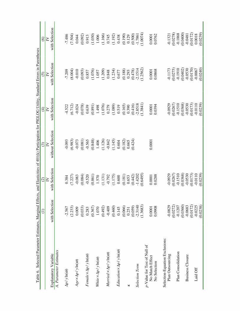
Tab
le 6
. S
elec
ted
Par
amet
er E
stim
ates
, M
argin
al E
ffec
ts,
and
Ela
stic
itie
s o
f 4
01
(k)
Par
tici
pat
ion f
or
PIG
LO
G U
tili
ty,
Sta
nd
ard
Err
ors
in P
aren
thes
es
(1
) (2
) (3
) (4
) (5
) (6
)
Exp
lanat
ory
Var
iab
le
w
ith S
elec
tio
n
IV
wit
h S
elec
tio
n
IV
wit
ho
ut
Sel
ecti
on
IV
wit
h S
elec
tio
n
IV
wit
h S
elec
tio
n
IV
wit
h S
elec
tio
n
A.
Pa
ram
eter
Est
ima
tes
)ln
(/
ωy
p∆
-2
.56
7
0.3
84
-0
.09
3
-4.5
22
-7
.20
9
-7.4
86
(2
.233
) (7
.227
) (6
.983
) (6
.712
) (8
.004
) (7
.504
)
)ln
(/
ωy
pA
ge
∆×
0
.00
9
-0.0
83
-0
.07
3
-0.0
24
-0
.01
0
0.0
44
(0
.033
) (0
.084
) (0
.081
) (0
.078
) (0
.093
) (0
.092
)
)ln
(/
ωy
pF
ema
le∆
×
0.2
83
-0
.52
0
-0.5
65
0
.63
9
0.8
57
0
.91
3
(0
.367
) (0
.861
) (0
.848
) (0
.891
) (1
.076
) (1
.030
)
)ln
(/
ωy
pW
hit
e∆
×
1.0
70
1
.57
0
1.4
06
1
.49
8
1.0
57
1
.00
6
(0
.492
) (1
.131
) (1
.126
) (1
.076
) (1
.209
) (1
.166
)
)ln
(/
ωy
pM
arr
ied
∆×
-0
.40
9
-0.7
92
-0
.84
2
0.2
79
0
.84
8
0.7
45
(0
.460
) (1
.175
) (1
.145
) (1
.089
) (1
.234
) (1
.192
)
)ln
(/
ωy
pE
du
cati
on
∆×
0
.14
5
0.6
00
0
.60
4
0.5
19
0
.67
7
0.4
38
(0
.066
) (0
.181
) (0
.182
) (0
.165
) (0
.188
) (0
.190
)
κ
0.2
51
0
.65
3
0.6
65
0
.39
0
0.2
93
0
.12
9
(0
.059
) (0
.442
) (0
.424
) (0
.416
) (0
.478
) (0
.500
) S
elec
tio
n T
erm
-2
.31
40
(1
.368
3)
-1.4
20
2
(0.6
49
5)
-2
.85
18
(1
.384
1)
-2.1
51
4
(1.2
56
2)
-1.7
86
1
(1.0
07
4)
p-V
alue
for
Tes
t o
f N
ull
of
N
o M
atch
Eff
ect
0.0
001
0
.00
01
0
.00
01
0
.00
01
0
.00
01
0
.00
01
No
Sel
ecti
on
0.0
908
0
.02
88
0.0
394
0
.08
68
0
.07
62
Sel
ecti
on
-Eq
uat
ion E
xcl
usi
on
s:
Pla
n O
uts
ourc
ing
-0.0
82
9
-0.0
92
9
-0
.09
29
-0
.11
73
-0
.13
21
(0.0
27
2)
(0.0
26
7)
(0
.026
7)
(0.0
27
5)
(0.0
27
8)
Pla
n C
onso
lid
atio
n
-0.1
20
7
-0.1
51
0
-0
.15
10
-0
.19
10
-0
.18
68
(0.0
36
0)
(0.0
36
8)
(0
.036
8)
(0.0
40
2)
(0.0
40
0)
Busi
nes
s C
losu
re
-0.0
68
3
-0.0
53
0
-0
.05
30
-0
.05
30
-0
.04
81
(0.0
17
2)
(0.0
17
3)
(0
.017
3)
(0.0
17
0)
(0.0
17
2)
Lai
d O
ff
-0.0
22
5
-0.0
11
0
-0
.01
10
-0
.00
67
0
.00
18
(0.0
23
8)
(0.0
23
9)
(0
.023
9)
(0.0
24
0)
(0.0
23
9)

67
(1
) (2
) (3
) (4
) (5
) (6
) B
. A
dd
itio
na
l C
on
tro
ls
F
rin
ge
Ben
efit
, an
d P
lan
Char
acte
rist
ics?
N
o
No
N
o
Yes
Y
es
Yes
Inte
ract
ion o
f fi
rm s
ize
wit
h F
ringe
Ben
efit
s an
d P
lan c
har
acte
rist
ics
No
N
o
No
N
o
Yes
Y
es
Occ
up
atio
n a
nd
Inte
ract
ion
s o
f O
ccup
atio
n w
ith D
emo
gra
ph
ics,
F
rin
ge
Ben
efit
s, P
lan C
har
acte
rist
ics,
an
d O
ther
Em
plo
ym
ent
Char
acte
rist
ics?
No
N
o
No
N
o
No
Y
es
C.
Ma
rgin
al
Eff
ect
on
Pro
ba
bil
ity
of
Pa
rtic
ipa
tio
n w
ith
Res
pec
t to
M
atch
Rat
e
(ad
dit
ional
$1
per
$1 c
ontr
ibute
d)
0.0
091
0
.26
95
0
.47
24
0
.09
44
0
.18
33
0
.19
97
V
irtu
al F
ull
Inco
me
(a
dd
itio
nal
$1
00,0
00
) -0
.00
27
-0
.08
07
-0
.02
83
-0
.05
49
-0
.05
98
-0.1
41
6
Net
Wag
e (a
dd
itio
nal
$1
per
ho
ur)
-0
.00
01
-0
.00
26
-0
.00
46
-0
.00
09
-0
.00
18
-0
.00
19
M
argin
al T
ax R
ate
(incr
ease
of
10
per
centa
ge
po
ints
) 0
.00
05
0
.01
58
0
.02
78
0
.00
56
0
.01
08
0
.01
17
Pre
dic
ted
Pro
bab
ilit
y o
f P
arti
cip
atio
n
0.9
7
0.8
6
0.5
7
0.9
4
0.8
8
0.8
1
D
. P
art
icip
ati
on
Ela
stic
ity
wit
h R
esp
ect
to
M
atch
Rat
e 0
.00
46
0
.07
11
0
.19
50
0
.02
28
0
.04
73
0
.05
61
Full
Inco
me
-0.0
03
2
-0.1
03
9
-0.2
84
9
-0.0
33
3
-0.0
69
1
-0.0
81
9

68
(1
) (2
) (3
) (4
) (5
) (6
)
Net
Wag
e -0
.00
12
-0
.04
11
-0
.11
26
-0
.01
32
-0
.02
73
-0
.03
24
Mar
gin
al T
ax R
ate
0.0
013
0
.04
34
0
.11
89
0
.01
39
0
.02
88
0
.03
42
No
te:
Co
lum
ns
1-6
of
Pan
el A
of
this
tab
le p
rese
nt
par
amet
er e
stim
ates
of
(18
) in
the
tex
t.
Fo
r al
l co
lum
ns,
the
sam
ple
co
nsi
sts
of
1,0
42
ind
ivid
ual
s.
All
the
colu
mn
s ex
cep
t th
e fi
rst
assu
me
pri
ces,
net
wag
e, a
nd
vir
tual
inco
me
are
end
ogen
ous.
Co
lum
ns
2 a
nd
4-6
pre
sent
sele
ctio
n-c
orr
ecte
d e
stim
ates
usi
ng t
he
excl
usi
on r
estr
icti
on
s d
iscu
ssed
in t
he
text
and
the
app
end
ix.
The
par
amet
er e
stim
ates
fo
r th
e se
lect
ion t
erm
in t
he
par
tici
pat
ion e
quat
ion a
re s
ho
wn i
n P
anel
A.
Pan
el A
als
o p
rese
nts
p
aram
eter
est
imat
es f
or
the
excl
usi
on r
estr
icti
ons
fro
m t
he
sele
ctio
n e
quat
ion
s. T
he
esti
mat
es i
n c
olu
mn 3
are
no
t se
lect
ion c
orr
ecte
d.
Pan
el B
pre
sents
the
add
itio
nal
co
ntr
ols
incl
ud
ed.
Mar
gin
al e
ffec
ts e
val
uat
ed a
t th
e m
ean o
f th
e re
gre
sso
rs a
re s
ho
wn i
n p
anel
C.
Pan
el D
pre
sents
est
imat
es o
f el
asti
citi
es o
f 4
01
(k)
par
tici
pat
ion
bas
ed o
n t
he
par
amet
er e
stim
ates
in p
anel
A,
eval
uat
ed a
t th
e sa
mp
le m
ean
s.

69
Tab
le 7
. E
stim
ated
Mar
gin
al E
ffec
ts a
nd
Ela
stic
itie
s fo
r P
IGL
OG
Uti
lity
by D
emo
gra
ph
ic G
roup
s
(1
) (2
) (3
) (4
) (5
) (6
) (7
)
Mea
sure
Mal
e
Fem
ale
Hig
h S
cho
ol
Dro
po
ut
Hig
h S
cho
ol
Dip
lom
a S
om
e C
oll
ege
Co
lleg
e D
egre
e G
rad
uat
e S
cho
ol
Par
tici
pat
ion M
argin
al E
ffec
t
0.2
259
0.1
750
0
.06
70
0
.17
25
0
.21
77
0
.25
32
0
.26
33
fr
om
the
Mat
ch R
ate
P
arti
cip
atio
n E
last
icit
y w
ith
Res
pec
t to
the
Mat
ch R
ate
0.0
490
0.0
188
0
.04
84
0
.06
10
0
.07
10
0
.07
38
0
.04
90
No
te:
This
tab
le s
ho
ws
esti
mat
ed m
argin
al e
ffec
ts a
nd
ela
stic
itie
s o
f co
ntr
ibuti
on
s w
ith r
esp
ect
to t
he
emp
loyer
mat
ch r
ate
by s
ex a
nd
ed
uca
tio
n g
roup
bas
ed o
n t
he
par
amet
er e
stim
ates
fro
m t
he
rich
est
spec
ific
atio
n,
sho
wn i
n c
olu
mn 6
of
Tab
le 6
, ev
aluat
ed a
t th
e sa
mp
le
mea
ns.

70
Tab
le 8
. S
elec
ted
Par
amet
er E
stim
ates
, M
argin
al E
ffec
ts,
and
E
last
icit
ies
fro
m B
ox-C
ox U
tili
ty F
unct
ion,
C
orr
ecti
ng f
or
Sel
ecti
on a
nd
End
ogen
eity
, S
tand
ard
Err
ors
in P
aren
thes
es
Mea
sure
(1
) (2
) (3
) (4
)
A.
Pa
ram
eter
Est
ima
tes
λ
-0.1
97
0
(0.0
94
5)
-0.3
10
8
(0.1
50
3)
-0.2
53
4
(0.1
33
4)
-0.3
53
4
(0.1
85
9)
S
elec
tio
n T
erm
-0
.63
34
(0
.277
7)
-0.6
33
2
(0.2
70
4)
-0.4
82
0
(0.2
90
1)
-0.4
03
0
(0.2
80
5)
p-V
alue
for
Tes
t o
f N
ull
of
N
o M
atch
Eff
ect
0.0
001
0
.00
01
0
.00
01
0
.00
01
No
Sel
ecti
on
0.0
228
0
.01
94
0
.09
70
0
.15
12
Ela
stic
ity
of
Inte
rtem
po
ral
Sub
stit
uti
on
0
.83
44
0
.76
29
0
.79
78
0
.73
86
B.
Ad
dit
iona
l C
on
tro
ls
F
rin
ge
Ben
efit
and
Pla
n C
har
acte
rist
ics?
N
o
Yes
Y
es
Yes
Inte
ract
ion o
f F
irm
Siz
e w
ith F
rin
ge
Ben
efit
s an
d P
lan C
har
acte
rist
ics?
N
o
No
Y
es
Yes
Occ
up
atio
n a
nd
Inte
ract
ion
s o
f O
ccup
atio
n w
ith D
emo
gra
ph
ics,
Fri
nge
Ben
efit
s, P
lan C
har
acte
rist
ics,
and
Oth
er E
mp
loym
ent
Char
acte
rist
ics?
N
o
No
N
o
Yes
C
. M
arg
ina
l E
ffec
t o
n t
he
Pro
ba
bil
ity
of
Pa
rtic
ipa
tio
n w
ith
Res
pec
t to
th
e
Mat
ch R
ate
0.0
706
0
.08
85
0
.11
50
0
.14
99
Full
Inco
me
-0.0
10
6
-0.0
07
4
-0.0
12
5
-0.0
08
1
N
et W
age
-0.0
00
3
-0.0
00
2
-0.0
00
3
-0.0
00
2
M
argin
al T
ax R
ate
0.0
287
0
.01
82
0
.03
07
0
.01
97
Pre
dic
ted
Pro
bab
ilit
y o
f P
arti
cip
atio
n
0.9
4
0.8
6
0.8
5
0.7
7

71
Mea
sure
(1
) (2
) (3
) (4
)
D.
Pa
rtic
ipa
tio
n E
last
icit
y w
ith
Res
pec
t to
th
e
Mat
ch R
ate
0.0
170
0
.02
33
0
.03
06
0
.04
48
Full
Inco
me
-0.0
16
6
-0.0
12
8
-0.0
21
8
-0.0
15
6
N
et W
age
-0.0
06
5
-0.0
05
0
-0.0
08
5
-0.0
06
1
M
argin
al T
ax R
ate
0.0
150
0
.01
17
0
.01
99
0
.01
41
No
te:
Co
lum
ns
1-4
of
Pan
el A
of
this
tab
le p
rese
nt
sele
cted
par
amet
er e
stim
ates
fro
m (
18
) in
the
text
allo
win
g λ
to
var
y u
sing n
on
-lin
ear
max
imu
m l
ikel
iho
od
.
Fo
r al
l co
lum
ns,
the
sam
ple
co
nsi
sts
of
1,0
42
ind
ivid
ual
s.
All
the
colu
mn
s as
sum
e p
rice
s, n
et w
age,
and
vir
tual
inco
me
are
end
ogen
ous,
and
co
rrec
t fo
r en
do
gen
eity
usi
ng t
he
sam
e in
stru
men
tal
var
iab
les
as u
sed
in t
he
linea
r m
axim
um
lik
elih
oo
d e
stim
atio
n i
n T
able
6.
All
co
lum
ns
corr
ect
for
po
ssib
le n
on-r
and
om
se
lect
ion
in
to t
he
sam
ple
usi
ng t
he
sam
e ex
clusi
on
s as
in T
able
6.
The
esti
mat
es o
f th
e el
asti
city
of
inte
rtem
po
ral
sub
stit
uti
on
sho
wn
ab
ove
are
actu
ally
neg
ativ
e b
ut
are
exp
ress
ed i
n a
bso
lute
val
ue
to f
acil
itat
e co
mp
aris
on
to
tho
se f
rom
the
con
sum
pti
on E
ule
r-eq
uat
ion l
iter
ature
. P
anel
B p
rese
nts
the
add
itio
nal
co
ntr
ols
in
clud
ed.
Mar
gin
al e
ffec
ts e
val
uat
ed a
t th
e m
ean o
f th
e re
gre
sso
rs a
re s
ho
wn i
n p
anel
C.
Pan
el D
pre
sents
est
imat
es o
f el
asti
citi
es o
f 4
01
(k)
par
tici
pat
ion b
ased
o
n t
he
par
amet
er e
stim
ates
in p
anel
A,
eval
uat
ed a
t th
e sa
mp
le m
ean
s.

F
igu
re 1
2C
f
h
)1
/()
1)(
1(sl
ope
12
FF
rθ
θ−
+−
−=
i
k
c
d
)1
/()
1)(
1)(
1(sl
ope
12
FV
OL
Fr
mθ
θ−
++
−−
=
vy
2
vy 1
b
SS
FW
r)
1)(
1(2
+−
θ
a
max
Q
ma
tch
Q
1
C
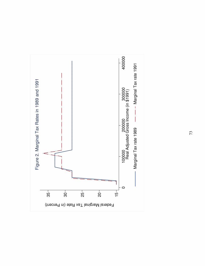
73
15
20
25
30
35
Federal Marginal Tax Rate (in Percent)
010
00
00
20
00
00
30
00
00
40
00
00
Re
al A
dju
ste
d G
ross Inco
me
(in
$19
91
)
Ma
rgin
al T
ax r
ate
198
9M
arg
ina
l Tax r
ate
199
1
Fig
ure
2.
Ma
rgin
al T
ax R
ate
s in
19
89
an
d 1
99
1