Gamma: C++ Generic Synthesis Library

Tutorial

Version 0.9.5

April 5, 2012

Author: Lance Putname-mail: putnam.lance@gmail.com

Contents

1 Gamma Overview 21.1 Generic Types . . . . . . . . . . . . . . . . . . . . . . . . . . . . . . . . . . . . . . . . . . . . . . 21.2 Generators and Filters . . . . . . . . . . . . . . . . . . . . . . . . . . . . . . . . . . . . . . . . . 21.3 Domain Synchronization . . . . . . . . . . . . . . . . . . . . . . . . . . . . . . . . . . . . . . . . 2

2 Obtaining and Building 32.1 Linux Compilation . . . . . . . . . . . . . . . . . . . . . . . . . . . . . . . . . . . . . . . . . . . 32.2 Mac OSX Compilation . . . . . . . . . . . . . . . . . . . . . . . . . . . . . . . . . . . . . . . . . 42.3 Windows Compilation . . . . . . . . . . . . . . . . . . . . . . . . . . . . . . . . . . . . . . . . . 42.4 Building With Make . . . . . . . . . . . . . . . . . . . . . . . . . . . . . . . . . . . . . . . . . . 4

3 Gamma Objects 43.1 Generators . . . . . . . . . . . . . . . . . . . . . . . . . . . . . . . . . . . . . . . . . . . . . . . . 43.2 Filters . . . . . . . . . . . . . . . . . . . . . . . . . . . . . . . . . . . . . . . . . . . . . . . . . . . 93.3 Spectral Processing . . . . . . . . . . . . . . . . . . . . . . . . . . . . . . . . . . . . . . . . . . . 123.4 Effects . . . . . . . . . . . . . . . . . . . . . . . . . . . . . . . . . . . . . . . . . . . . . . . . . . . 133.5 I/O . . . . . . . . . . . . . . . . . . . . . . . . . . . . . . . . . . . . . . . . . . . . . . . . . . . . 143.6 Event Scheduling . . . . . . . . . . . . . . . . . . . . . . . . . . . . . . . . . . . . . . . . . . . . 17

4 Related Work 194.1 Other C++ Synthesis Libraries . . . . . . . . . . . . . . . . . . . . . . . . . . . . . . . . . . . . . 194.2 Readings . . . . . . . . . . . . . . . . . . . . . . . . . . . . . . . . . . . . . . . . . . . . . . . . . 20

1

1 Gamma Overview

Gamma is a cross-platform, C++ library for doing generic synthesis and filtering of numerical data. Itcontains numerous mathematical functions related to synthesis together with an assortment of sequencegenerators and filters for signal processing. It is oriented towards real-time sound and graphics rendering,but is equally useful for non-real-time tasks.

1.1 Generic Types

Gamma objects are templated on their value type allowing them to be used with any arithmetic data types,such as scalars, vectors, and complex numbers. Processing algorithms are designed as much as possibleto be data type and domain independent. This allows a common set of functions and objects to be usedfor a variety of modalities, such as sound or graphics, and in arbitrary domains, such as time, space, orfrequency. Algorithms are type generic which means they can process any type of data that has the appro-priate mathematical operators defined (typically +, -, *, and /). The following illustrates how a variety ofsequence generators can be constructed from a generic recursive multiplication class, RMul:

RMul<float > rMul(0.99); // decaying envelope

RMul<Vec3<> > rMul(Vec3<>(0.9,0.8,0.7)); // 3 decaying envelopes

RMul<Complex<> > rMul(Polar<>(1.00, M_2PI/8)); // complex sinusoid

RMul<Complex<> > rMul(Polar<>(0.99, M_2PI/8)); // complex exponential

1.2 Generators and Filters

Processing objects are typically either a generator or a filter and can be either domain observers or not.Objects adopt a standard processing operator interface similar to functional syntax. Generators return theirnext value with the () operator and filters return their next value with the (T) operator, where T is a valuetype.

gen::RAdd rAdd(1, 0); // recursively add 1 starting at 0

for(int i=0; i<4; ++i) cout << rAdd(); // prints "1 2 3 4"

fil::Delay1 delay1(0); // 1 element delay starting with 0

for(int i=1; i<5; ++i) cout << delay1(i); // prints "0 1 2 3"

1.3 Domain Synchronization

A sampling domain is a discretely-spaced independent variable along which a function is evaluated. InGamma, domains are abstracted through an observer design pattern into a Sync subject and a Synced

observer. The Sync holds a sampling rate/interval amount and notifies its attached Synceds wheneverit changes value. The following example shows how we can create an audio sample rate subject with anobserver:

2

struct MySynced : public Synced {

// This is called whenever the sampling domain changes

// ’dr’ is the new SPU divided by the old SPU

void onResync(double dr);

};

Sync sync;

sync.spu(44100); // set samples/unit (in our case 44,100 samples/sec)

MySynced synced;

synced.spu(); // returns 1 (the default)

sync << synced; // make ’synced’ an observer of ’sync’

synced.spu(); // returns 44,100

sync.spu(8000); // change the sample rate, calls onResync of ’synced’

synced.spu(); // returns 8000

2 Obtaining and Building

The Gamma source code can be downloaded from http://mat.ucsb.edu/gamma/. This is where to get themost recent stable releases. To obtain a more current, but possibly (and most likely) unstable version, youcan check out the source anonymously through SVN via

svn co https://svn.mat.ucsb.edu/svn/gamma/trunk gamma

The simplest way to build the library is to use GNU Make. Instructions for setting up each platformwith Make follow. Further instructions can be found in the README file in the root directory.

2.1 Linux Compilation

The simplest way to build the library is to use GNU Make (see section 2.4 below). Use either Synaptic orapt-get to install the most recent developer versions of libsndfile and PortAudio (v19). If using apt-get,you will do something like

sudo apt-get update

sudo apt-get install portaudio19-dev libsndfile1-dev

Gamma has also been tested to work with Puredyne, a Linux live CD distribution that convenientlybundles with it the important media-related libraries. Unfortunately, it does not come with g++ installed,so you have to install it manually on boot-up:

sudo apt-get update

sudo apt-get install g++-4.4

3

2.2 Mac OSX Compilation

You can build the library using either GNU Make or Xcode. If you are using Make, see section 2.4 below. Touse Xcode, you will need to install the developer tools from Apple. You can get them for free (after registra-tion) from http://developer.apple.com/. The Xcode project is located at project/xcode/gamma.xcodeproj.

2.3 Windows Compilation

There is currently no provided Visual Studio project. Visual Studio Express can be downloaded for freefrom Microsoft. It will be necessary to link to libsndfile and PortAudio v19. Alternatively, you can useCygwin or MinGW which provide a Linux-like environment natively from within Windows. They canbe used to build the Gamma sources using their provided version of GNU Make. These methods have notbeen thoroughly tested, so you can contribute to Gamma if you inform the author of your working solution.

2.4 Building With Make

If you had to install Make, test that it is working by opening a terminal and typing ’make –version’. Beforerunning Make, ensure that the correct build options are set in the file Makefile.config. These can beset directly in Makefile.config or passed in as options to Make as OPTION=value. If you are usingLinux/Puredyne, you will also need to uncomment the line USING_PUREDYNE = 1. To build the Gammalibrary, run make and hope for the best.

3 Gamma Objects

3.1 Generators

Generators produce a continuous stream of samples such as a periodic function or a continuous curve.They are function objects in that they store some internal state and act just like a mathematical function, bothsyntactically and semantically. Given some generator, g, we can command it to generate its next sampleby calling g(). Note that this call looks and acts just like a nullary mathematical function, that is, g is thefunction and g() evaluates the function returning its output. It differs from a function, however, in thatit may return a different value each time it is called. Since generators are also objects, many also haveparameters to control their output. The following code example shows a typical use case of a generator,Gen, setting its parameters and generating samples.

Gen g; // define a new generator

g.freq(100); // set its frequency parameter

g.phase(0.25); // set its phase parameter

float v;

v = g(); // generate first sample

v = g(); // generate second sample

Since generators simply return a sample when evaluated, one can form algebraic expressions with themusing standard C++ operators. The next example shows how two oscillators can be summed together and

4

then multiplied by an envelope.

Osc osc1, osc2; // define two oscillators

Env env; // define an envelope

float v;

v = (osc1() + osc2()) * env(); // generate first sample

v = (osc1() + osc2()) * env(); // generate second sample

Oscillators

[generator/(oscAccum, oscSweep, oscLFO1, oscLFO2, oscOsc, oscImpulse)]Oscillators produce a periodic waveform with adjustable phase and frequency. They typically have

freq() and phase() methods for setting their frequency and phase.Accum accumulates an internal fixed-point phase at a specified frequency. Requiring only a single fixed-

point addition per iteration, it is the fastest generator. It can be used as a timer or as the input to a wave-shaping table or function. Sweep is an Accum that cycles linearly through the interval [0, 1) at a specifiedfrequency.

Sine is the “go to” sine wave oscillator. It produces a high-quality sine wave using a polynomialapproximation.

LFO (low-frequency oscillator) produces various piece-wise polynomial waveforms derived from thephase of an Accum. Since the waveforms are not band-limited, they should only be used as low-frequencymodulation sources. Figure 1 shows the static waveforms that can be produced.

(a) imp (b) down (c) up

(d) sqr (e) tri (f) para

(g) cos (h) even3 (i) even5

Figure 1: LFO static waveforms (two cycles shown)

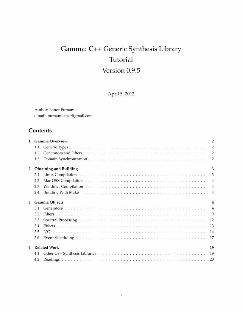
Figure 2 shows the dynamic waveforms whose shape can be changed smoothly with the mod parameter.

5

(a) pulse (mod u 0) (b) pulse (mod = 1/4) (c) pulse (mod = 2/4) (d) pulse (mod = 3/4)

(e) stair (mod = 0/8) (f) stair (mod = 1/8) (g) stair (mod = 2/8) (h) stair (mod = 3/8)

(i) up2 (mod = 0/4) (j) up2 (mod = 1/4) (k) up2 (mod = 2/4) (l) up2 (mod = 3/4)

(m) line2 (mod = 0/4) (n) line2 (mod = 1/4) (o) line2 (mod = 2/4) (p) line2 (mod = 3/4)

Figure 2: LFO dynamic waveforms (two cycles shown)

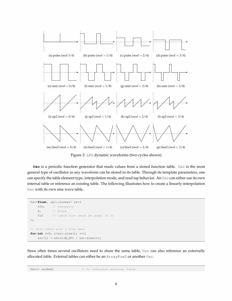
Osc is a periodic function generator that reads values from a stored function table. Osc is the mostgeneral type of oscillator as any waveform can be stored in its table. Through its template parameters, onecan specify the table element type, interpolation mode, and read tap behavior. An Osc can either use its owninternal table or reference an existing table. The following illustrates how to create a linearly-interpolationOsc with its own sine wave table.

Osc<float, ipl::Linear> src(

100, // frequency

0, // phase

512 // table size (must be power of 2)

);

// fill table with a sine wave

for(int i=0; i<src.size(); ++i)

src[i] = sin(i*M_2PI / src.size());

Since often times several oscillators need to share the same table, Osc can also reference an externallyallocated table. External tables can either be an ArrayPow2 or another Osc.

Osc<> oscRef; // to reference external table

6

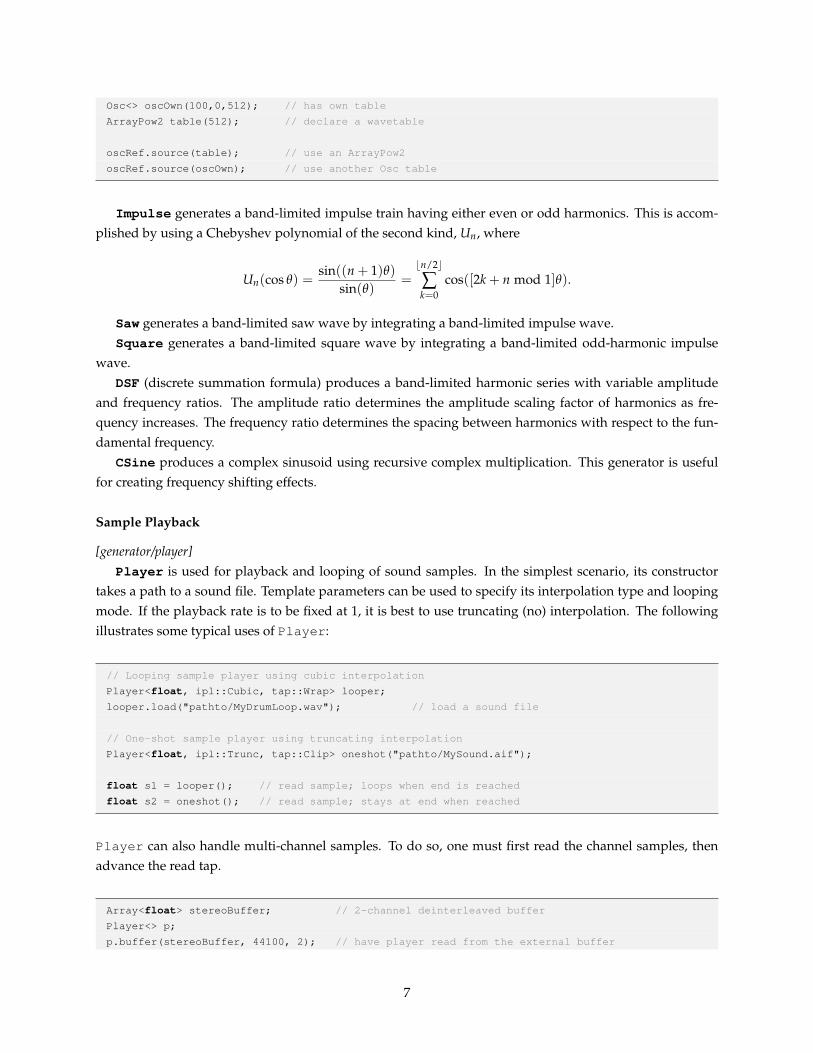
Osc<> oscOwn(100,0,512); // has own table

ArrayPow2 table(512); // declare a wavetable

oscRef.source(table); // use an ArrayPow2

oscRef.source(oscOwn); // use another Osc table

Impulse generates a band-limited impulse train having either even or odd harmonics. This is accom-plished by using a Chebyshev polynomial of the second kind, Un, where

Un(cos θ) =sin((n + 1)θ)

sin(θ)=bn/2c

∑k=0

cos([2k + n mod 1]θ).

Saw generates a band-limited saw wave by integrating a band-limited impulse wave.Square generates a band-limited square wave by integrating a band-limited odd-harmonic impulse

wave.DSF (discrete summation formula) produces a band-limited harmonic series with variable amplitude

and frequency ratios. The amplitude ratio determines the amplitude scaling factor of harmonics as fre-quency increases. The frequency ratio determines the spacing between harmonics with respect to the fun-damental frequency.

CSine produces a complex sinusoid using recursive complex multiplication. This generator is usefulfor creating frequency shifting effects.

Sample Playback

[generator/player]Player is used for playback and looping of sound samples. In the simplest scenario, its constructor

takes a path to a sound file. Template parameters can be used to specify its interpolation type and loopingmode. If the playback rate is to be fixed at 1, it is best to use truncating (no) interpolation. The followingillustrates some typical uses of Player:

// Looping sample player using cubic interpolation

Player<float, ipl::Cubic, tap::Wrap> looper;

looper.load("pathto/MyDrumLoop.wav"); // load a sound file

// One-shot sample player using truncating interpolation

Player<float, ipl::Trunc, tap::Clip> oneshot("pathto/MySound.aif");

float s1 = looper(); // read sample; loops when end is reached

float s2 = oneshot(); // read sample; stays at end when reached

Player can also handle multi-channel samples. To do so, one must first read the channel samples, thenadvance the read tap.

Array<float> stereoBuffer; // 2-channel deinterleaved buffer

Player<> p;

p.buffer(stereoBuffer, 44100, 2); // have player read from the external buffer

7

float s1 = p.read(0); // read left channel sample

float s2 = p.read(1); // read right channel sample

p.advance(); // advance read tap

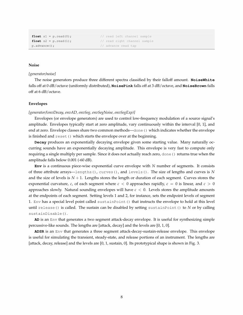
Noise

[generator/noise]The noise generators produce three different spectra classified by their falloff amount. NoiseWhite

falls off at 0 dB/octave (uniformly distributed), NoisePink falls off at 3 dB/octave, and NoiseBrown fallsoff at 6 dB/octave.

Envelopes

[generator/(envDecay, envAD, envSeg, envSegNoise, envSegExp)]Envelopes (or envelope generators) are used to control low-frequency modulation of a source signal’s

amplitude. Envelopes typically start at zero amplitude, vary continuously within the interval [0, 1], andend at zero. Envelope classes share two common methods—done() which indicates whether the envelopeis finished and reset() which starts the envelope over at the beginning.

Decay produces an exponentially decaying envelope given some starting value. Many naturally oc-curring sounds have an exponentially decaying amplitude. This envelope is very fast to compute onlyrequiring a single multiply per sample. Since it does not actually reach zero, done() returns true when theamplitude falls below 0.001 (-60 dB).

Env is a continuous piece-wise exponential curve envelope with N number of segments. It consistsof three attribute arrays—lengths(), curves(), and levels(). The size of lengths and curves is Nand the size of levels is N + 1. Lengths stores the length or duration of each segment. Curves stores theexponential curvature, c, of each segment where c < 0 approaches rapidly, c = 0 is linear, and c > 0approaches slowly. Natural sounding envelopes will have c < 0. Levels stores the amplitude amountsat the endpoints of each segment. Setting levels 1 and 2, for instance, sets the endpoint levels of segment1. Env has a special level point called sustainPoint() that instructs the envelope to hold at this leveluntil release() is called. The sustain can be disabled by setting sustainPoint() to N or by callingsustainDisable().

AD is an Env that generates a two segment attack-decay envelope. It is useful for synthesizing simplepercussive-like sounds. The lengths are [attack, decay] and the levels are [0, 1, 0].

ADSR is an Env that generates a three segment attack-decay-sustain-release envelope. This envelopeis useful for simulating the transient, steady-state, and release portions of an instrument. The lengths are[attack, decay, release] and the levels are [0, 1, sustain, 0]. Its prototypical shape is shown in Fig. 3.

8

A Dt

R

amp

S

Figure 3: An ADSR prototypical envelope shape.

Seg generates an envelope by interpolating between a sequence of breakpoints. A Seg can be used todownsample another generator, such as a noise generator, to produce a more slowly varying curve. Thefollowing example shows how to create a noise signal made of line segments (AKA band-limited noise):

Seg<float, iplSeq::Linear> seg(1.); // linear segment with length of 1

NoiseWhite<> noise; // white (uniform) noise generator

float s = seg(noise); // generate next linear-piecewise white noise

SegExp is like Seg but generates an exponential curve between breakpoints.

3.2 Filters

[filter/freqResponses]A filter applies a particular transformation to a stream of input samples to produce a new stream of

output samples. Filters behave identically to the generators discussed above (3.1) with one important dif-ference—they act like unary functions rather than nullary functions. The following example shows howthe output of a generator is filtered.

Gen g; // define a generator

Filter f; // define a filter

float v;

v = g(); // generate first sample

v = f(v); // filter first sample

v = f(g()); // generate and filter second sample

FIR

An FIR (finite impulse response) filter produces new values from a linear combination of its previous inputs.It is relatively easy to construct FIR filters with a linear-phase response by using symmetrical coefficients.Linear-phase responses have the desirable characteristic of not distorting the phase of the input signal.The disadvantage of FIR filters is that very high orders are required to obtain steep frequency responses.

9

Because of this, it often becomes necessary to implement FIRs using an FFT.MovingAvg is a moving average filter that outputs the average of its previous N input values. It acts

as a low-pass filter and does very well at preserving the shape of the input signal (due to its linear-phaseresponse). It is quite unique amongst FIRs in that it can be implemented with computational complexityO(1), independent of its order. Plots of its frequency response magnitude are shown in Fig. 4.

Figure 4: MovingAvg frequency response magnitudes for orders N = 1, 3, 10 (left to right).

Notch is a two-zero notch filter with linear-phase. The notch center frequency, fc, can be controlled, butits bandwidth cannot. Plots of its frequency response magnitude are shown in Fig. 5. As can be seen, whenfc < fs/4, the filter has a high-pass characteristic and when fc > fs/4, it has a low-pass characteristic.

Figure 5: Notch frequency response magnitudes for orders fc =18 fs, 1

4 fs, 38 fs (left to right).

IIR

[filter/(onePole, biquad, blockDC)]An IIR (infinite impulse response) filter produces new values from a linear combination of its previous

inputs and outputs. IIRs can produce steep “ringing” frequency responses much more efficiently than FIRs.Their main disadvantage is that they have a non-linear phase response which can smear sharp transients inthe input signal if one is not careful. Also, higher-order filters are generally not numerically stable so onetypically needs to cascade several first- or second-order filters in series.

OnePole is a single pole filter that is useful for smoothing and integrating signals. The cut-off frequencyis the frequency at which the magnitude spectrum is -3 dB. Some plots of its frequency response magnitudeare shown in Fig. 6.

Figure 6: OnePole frequency response magnitudes for fc = 0.22 fs, 0.11 fs, 0.05 fs (left to right).

Biquad is a general-purpose second-order IIR filter. It conveniently provides resonant filter designsthat can operate in low-pass, high-pass, band-pass, band-reject, or all-pass modes. The resonance amountcontrols the “presence” or steepness of the filter at its center frequency. For the low- and high-pass varieties,resonance is proportional to the amount of ringing at the center frequency. A resonance setting of 1 resultsin a maximally-flat pass band without ringing, i.e. a Butterworth filter. For the band-pass and -reject vari-eties, resonance is inversely proportional to the band-width of the filter. For the all-pass variety, resonancecontrols the locality of the phase distortion at the center frequency.

10

BlockDC is used for eliminating DC bias from signals. Sometimes very low frequency componentswill sneak into a signal, i.e., from positive feedback loops, which can create unwanted distortion due toclipping on the DAC. A BlockDC can be put at the end of the signal chain to eliminate these low-frequencycomponents without coloring the rest of the signal.

Allpass1 is a first-order all-pass filter. Allpass1 acts like a single-sample delay, however, the delayfor each frequency component can be a fractional amount less than 1. The phase is shifted from 0 to 180degrees going from DC to Nyquist. The center frequency is the frequency where the phase is shifted by 90degrees. It is easy to construct 1-pole/1-zero low- and high-pass filters by adding or subtracting, respec-tively, the output of Allpass1 from the input. The low- and high-pass filters are very similar to 1-polefilters, but have a sharper fall-off as the magnitude goes to zero at Nyquist and DC, respectively. The high-pass filter can act as a DC blocker (identical to BlockDC) at low cutoff. For convenience, these filters areimplemented as the methods low() and high().

Allpass2 is a second-order all-pass filter. Allpass2 creates a frequency-dependent phase transi-tion from 0 to 360 degrees going from DC to Nyquist. The center frequency is the frequency where thephase is shifted by 180 degrees. It is easy to construct band-pass and -reject filters by adding or subtracting,respectively, the output of Allpass2 from the input.

Delay Lines

[filter/(delay, comb), effects/flanger]A delay line keeps a history of its previous inputs and/or outputs. Delay lines are very similar to FIR

and IIR filters, except they typically have a history several orders of magnitude higher, like 1000 samples.Delay is an all-pass filter whose only effect is to delay its input. Delays are starting points for build-

ing many different effects including vibrato, pitch-shifting, and reverberation. The delay time can be var-ied dynamically as there are several interpolation modes possible— ipl::Linear, ipl::Cubic, andipl::AllPass. If the delay time is not to be varied, then it is best to use either the ipl::Trunc oripl::AllPass modes as they will not color the magnitude spectrum. Delay has a write() methodto place a sample at the beginning of the delay-line and a read() method that returns samples in thedelay-line at specified delay amounts.

Delay<> delay(1., 0.1); // delay with max delay of 1 sec and delay of 0.1 sec

float s = ... // an input sample

float d;

d = delay(); // read delayed sample, d

delay(s); // write new sample, s, to delay

d = delay(s); // shorthand of the above

d = delay(); // feed scaled output back into input

delay(s + d*0.5); //

Comb is a special kind of delay line that operates more like an IIR filter. Comb filters are typical startingpoints for creating flanging, chorusing, echo, and reverberation effects. Feedforward creates notches in thespectrum while feedback creates resonant peaks. If the feedforward and feedback amounts are the same

11

magnitude, but opposite in sign, then an all-pass comb filter results. The delay time can be varied in asmooth way as with Delay.

Hilbert transform

[filter/HilbertFilter]Hilbert produces a complex-valued (analytic) signal from a real signal. Complex signals are required

to implement single-side band modulation effects. A frequency shift is accomplished by multiplying acomplex-valued signal (produced from a Hilbert filter) by a complex sinusoid whose frequency determinesthe amount of frequency shift.

3.3 Spectral Processing

Discrete Fourier Transform

[spectral/(RFFT, CFFT)]There are two classes for performing the discrete Fourier transform, RFFT for real-to-complex trans-

forms and CFFT for complex-to-complex transforms. The DFT can be any size, however, it will performbest when the size is a product of small primes (e.g., powers of two). Transforms occur in-place meaningthat the input and output sequences of the transform use the same memory. Single- and double-precisionfloating point are supported. For RFFT, the imaginary components at DC and Nyquist are zero and thusare not included in the output after a forward transform.

The following example demonstrates how to perform a forward and inverse transform using RFFT.

RFFT<float> dft(N);

float samples[N]; // real time/position samples

dft.forward(samples); // perform forward transform to complex frequency domain

samples[0]; // DC real component

samples[1]; // 1st harmonic real component

samples[2]; // 1st harmonic imaginary component

samples[3]; // 2nd harmonic real component

samples[4]; // 2nd harmonic imaginary component

...

samples[N-1]; // Nyquist real component

dft.inverse(samples); // transform back to real time/position domain

The following example demonstrates how to perform a forward and inverse transform using CFFT.

CFFT<float> dft(N);

Complex<float> samples[N]; // complex time/position samples

dft.forward(samples); // perform forward transform to complex frequency domain

samples[0]; // complex harmonic +0

samples[1]; // complex harmonic +1

...

samples[N-2]; // complex harmonic -2

12

samples[N-1]; // complex harmonic -1

dft.inverse(samples); // transform back to complex time/position domain

Short-time Fourier Transform

[spectral/STFT]The short-time Fourier transform uses overlapping windows to obtain better temporal resulotion and

to avoid discontinuities between analysis windows during resynthesis. The STFT object can operate in aspecial stream mode which hides buffering and allows easy insertion into a sample loop.

// Setup

STFT stft(

2048, // window size

2048/4, // hop size

0, // pad size

HANN, // window type: BARTLETT, BLACKMAN, BLACKMAN_HARRIS,

// HAMMING, HANN, WELCH, RECTANGLE

COMPLEX // format of frequency samples

);

// time-domain loop

{

float s = src();

// stream in samples until we have enough for a DFT

if(stft(s)){

// frequency domain loop

for(int k=0; k<stft.numBins(); ++k){

stft.bin(k); // the kth frequency sample

}

}

// stream out sample from overlap add resynthesis

s = stft();

}

3.4 Effects

Chorus

Chorus emulates multiple voices “singing” in unison (as in a choir) from a single source. Chorusing isuseful for thickening up otherwise dry and monotonous sounds. Chorus operates by mixing its input withthe input sent through two frequency modulated comb filters in parallel.

13

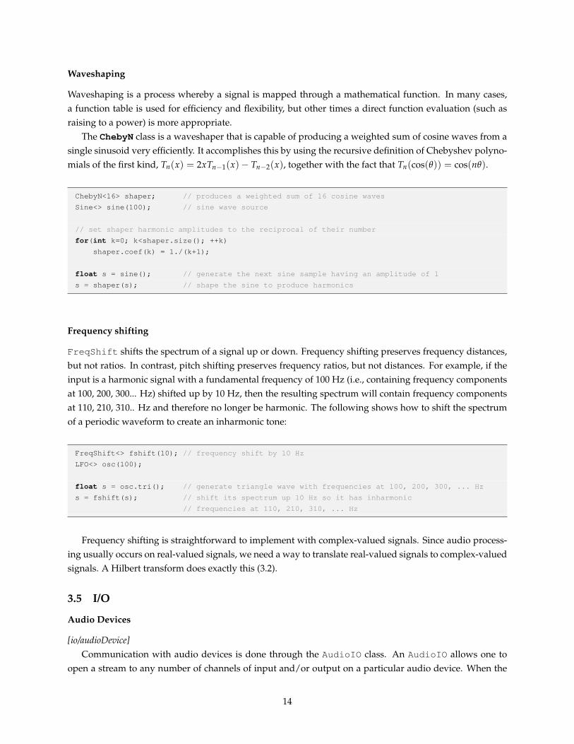
Waveshaping

Waveshaping is a process whereby a signal is mapped through a mathematical function. In many cases,a function table is used for efficiency and flexibility, but other times a direct function evaluation (such asraising to a power) is more appropriate.

The ChebyN class is a waveshaper that is capable of producing a weighted sum of cosine waves from asingle sinusoid very efficiently. It accomplishes this by using the recursive definition of Chebyshev polyno-mials of the first kind, Tn(x) = 2xTn−1(x)− Tn−2(x), together with the fact that Tn(cos(θ)) = cos(nθ).

ChebyN<16> shaper; // produces a weighted sum of 16 cosine waves

Sine<> sine(100); // sine wave source

// set shaper harmonic amplitudes to the reciprocal of their number

for(int k=0; k<shaper.size(); ++k)

shaper.coef(k) = 1./(k+1);

float s = sine(); // generate the next sine sample having an amplitude of 1

s = shaper(s); // shape the sine to produce harmonics

Frequency shifting

FreqShift shifts the spectrum of a signal up or down. Frequency shifting preserves frequency distances,but not ratios. In contrast, pitch shifting preserves frequency ratios, but not distances. For example, if theinput is a harmonic signal with a fundamental frequency of 100 Hz (i.e., containing frequency componentsat 100, 200, 300... Hz) shifted up by 10 Hz, then the resulting spectrum will contain frequency componentsat 110, 210, 310.. Hz and therefore no longer be harmonic. The following shows how to shift the spectrumof a periodic waveform to create an inharmonic tone:

FreqShift<> fshift(10); // frequency shift by 10 Hz

LFO<> osc(100);

float s = osc.tri(); // generate triangle wave with frequencies at 100, 200, 300, ... Hz

s = fshift(s); // shift its spectrum up 10 Hz so it has inharmonic

// frequencies at 110, 210, 310, ... Hz

Frequency shifting is straightforward to implement with complex-valued signals. Since audio process-ing usually occurs on real-valued signals, we need a way to translate real-valued signals to complex-valuedsignals. A Hilbert transform does exactly this (3.2).

3.5 I/O

Audio Devices

[io/audioDevice]Communication with audio devices is done through the AudioIO class. An AudioIO allows one to

open a stream to any number of channels of input and/or output on a particular audio device. When the

14

AudioIO is started, it will call a user supplied callback function at regular intervals. The rate at whichthe callback function is executed is the sample rate divided by the block size (both user specified). In thecallback, it is up to the user to read samples from the input buffer(s) and/or write samples to the outputbuffer(s). The argument to the callback function is a reference to an AudioIOData object which holds ontothe i/o buffers, user data, and other relevant information about the audio stream. Audio buffers are in anon-interleaved format so that samples within each channel are tightly packed.

The following code example illustrates how to open an audio stream to the default device and define acallback to process audio input.

#include "Gamma/AudioIO.h"

struct MyStuff{};

void audioCB(AudioIOData& io){

MyStuff& stuff = io.user<MyStuff>();

while(io()){

float inSample1 = io.in(0);

float inSample2 = io.in(1);

io.out(0) = -inSample1;

io.out(1) = -inSample2;

}

}

int main(){

MyStuff stuff;

AudioIO audioIO(

128, // block size

44100, // sample rate (Hz)

audioCB, // user-defined callback

&stuff, // user data

2, // input channels to open

2 // output

);

audioIO.start();

}

Sound Files

[io/soundFile]The SoundFile object is used to read/write various kinds of uncompressed sound file formats, such

as WAV, AIFF, AU, and FLAC. A sound file is usually comprised of a header describing the format (samplerate, amplitude resolution, compression algorithm), length (in samples), and number of channels of the datafollowed by a sequence of samples comprising the waveform of the sound. The data is most commonlystored in an interleaved format meaning that the samples iterate fastest over the channels, then over time.For example, an interleaved stereo sound would be stored as L1, R1, L2, R2, ..., LN , RN where Ln and Rn arethe left and right channel samples, respectively, at time n and N is the length of the sound. The following

15

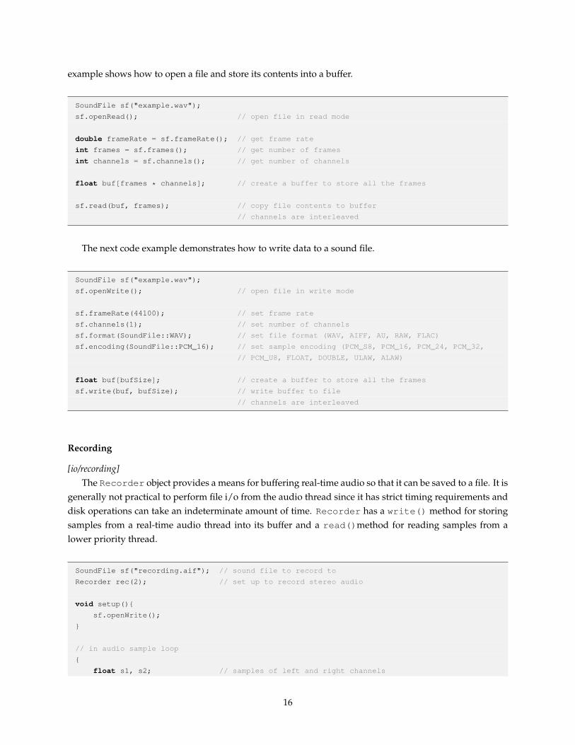
example shows how to open a file and store its contents into a buffer.

SoundFile sf("example.wav");

sf.openRead(); // open file in read mode

double frameRate = sf.frameRate(); // get frame rate

int frames = sf.frames(); // get number of frames

int channels = sf.channels(); // get number of channels

float buf[frames * channels]; // create a buffer to store all the frames

sf.read(buf, frames); // copy file contents to buffer

// channels are interleaved

The next code example demonstrates how to write data to a sound file.

SoundFile sf("example.wav");

sf.openWrite(); // open file in write mode

sf.frameRate(44100); // set frame rate

sf.channels(1); // set number of channels

sf.format(SoundFile::WAV); // set file format (WAV, AIFF, AU, RAW, FLAC)

sf.encoding(SoundFile::PCM_16); // set sample encoding (PCM_S8, PCM_16, PCM_24, PCM_32,

// PCM_U8, FLOAT, DOUBLE, ULAW, ALAW)

float buf[bufSize]; // create a buffer to store all the frames

sf.write(buf, bufSize); // write buffer to file

// channels are interleaved

Recording

[io/recording]The Recorder object provides a means for buffering real-time audio so that it can be saved to a file. It is

generally not practical to perform file i/o from the audio thread since it has strict timing requirements anddisk operations can take an indeterminate amount of time. Recorder has a write() method for storingsamples from a real-time audio thread into its buffer and a read()method for reading samples from alower priority thread.

SoundFile sf("recording.aif"); // sound file to record to

Recorder rec(2); // set up to record stereo audio

void setup(){

sf.openWrite();

}

// in audio sample loop

{

float s1, s2; // samples of left and right channels

16

... // generate samples

rec.write(s1, s2); // write stereo frame into buffer

}

// called periodically from non-audio thread

{

float * buf; // this will point to the read samples

int n = rec.read(buf); // copy samples from ring to read buffer

sf.write(buf, n); // write samples to the sound file

}

3.6 Event Scheduling

Gamma contains a very simple, yet flexible mechanism for scheduling and controlling processes withinthe audio thread from a separate lower-priority thread. The scheduling can be used to create synthesisgraphs, playback note lists, and do algorithmic composition in real-time. The two main components areScheduler and Process. Scheduler places new events into an order-of-execution tree of Processesthat are run from the audio thread. A Process is a user-defined audio processing unit which is typicallyeither a synth or an effect. To illustrate how these two components are used together, we will walkthroughhow to construct a very common synthesis network—a number of synthesizer voices running through aneffects chain. In our example, we will have a group voices with two voices, voice1 and voice2, anda group effects with two effects, chorus and reverb. We will use an order-of-execution tree that callsthe voices first and then runs their sum through the two effects in series. The tree is shown in Fig. 7. Theposition of each box is related to its child/sibling relationships in the tree and the solid arrows show theorder of execution. The tree is executed in a depth-first fashion so that children are visited first then siblings,if any, starting at the root node. When the end of a sibling chain is reached, we go back up the child chainuntil another sibling is found. When we make it back up the the root, then the trace is complete.

voice1 voice2

root

voices effects

chorus echo

child

sibling

Figure 7: Order-of-execution tree for a voice/effect synthesis network.

The code to set up and run the network is:

Scheduler s; // define a new scheduler

Process& effects = s.add<Process>(); // add effects group

Process& voices = s.add<Process>(); // add voices group

s.add<Echo>(effects); // add echo to effects

s.add<Chorus>(effects); // add chorus to effects

17

s.add<Voice>(voices).freq(220).dt(1); // add first voice to voices, starts after 1 second

s.add<Voice>(voices).freq(329.6); // add second voice to voices

s.start(); // start scheduler

AudioIO io(256, 44100., s.audioCB, &s); // define audio i/o

Sync::master().spu(io.fps()); // set sample rate

io.start(); // start audio i/o

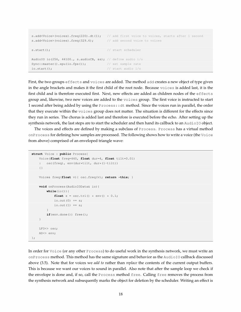
First, the two groups effects and voices are added. The method add creates a new object of type givenin the angle brackets and makes it the first child of the root node. Because voices is added last, it is thefirst child and is therefore executed first. Next, new effects are added as children nodes of the effectsgroup and, likewise, two new voices are added to the voices group. The first voice is instructed to start1 second after being added by using the Process::dt method. Since the voices run in parallel, the orderthat they execute within the voices group does not matter. The situation is different for the effects sincethey run in series. The chorus is added last and therefore is executed before the echo. After setting up thesynthesis network, the last steps are to start the scheduler and then hand its callback to an AudioIO object.

The voices and effects are defined by making a subclass of Process. Process has a virtual methodonProcess for defining how samples are processed. The following shows how to write a voice (the Voicefrom above) comprised of an enveloped triangle wave:

struct Voice : public Process{

Voice(float freq=440, float dur=4, float tilt=0.01)

: osc(freq), env(dur*tilt, dur*(1-tilt))

{}

Voice& freq(float v){ osc.freq(v); return *this; }

void onProcess(AudioIOData& io){

while(io()){

float s = osc.tri() * env() * 0.1;

io.out(0) += s;

io.out(1) += s;

}

if(env.done()) free();

}

LFO<> osc;

AD<> env;

};

In order for Voice (or any other Process) to do useful work in the synthesis network, we must write anonProcess method. This method has the same signature and behavior as the AudioIO callback discussedabove (3.5). Note that for voices we add to rather than replace the contents of the current output buffers.This is because we want our voices to sound in parallel. Also note that after the sample loop we check ifthe envelope is done and, if so, call the Process method free. Calling free removes the process fromthe synthesis network and subsequently marks the object for deletion by the scheduler. Writing an effect is

18

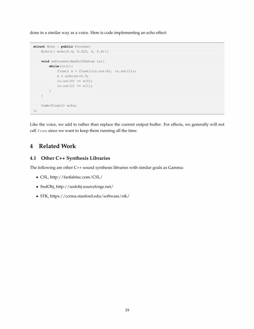
done in a similar way as a voice. Here is code implementing an echo effect:

struct Echo : public Process{

Echo(): echo(0.4, 0.323, 0, 0.8){}

void onProcess(AudioIOData& io){

while(io()){

float2 s = float2(io.out(0), io.out(1));

s = echo(s)*0.5;

io.out(0) += s[0];

io.out(1) += s[1];

}

}

Comb<float2> echo;

};

Like the voice, we add to rather than replace the current output buffer. For effects, we generally will notcall free since we want to keep them running all the time.

4 Related Work

4.1 Other C++ Synthesis Libraries

The following are other C++ sound synthesis libraries with similar goals as Gamma:

• CSL, http://fastlabinc.com/CSL/

• SndObj, http://sndobj.sourceforge.net/

• STK, https://ccrma.stanford.edu/software/stk/

19

Gamma 0.9.5 CSL 5 SndObj 2.6.6 STK 4.3.1

Spectral DFT, STFT DFT DFT, STFT, PV

Scalar proc. Yes No No Yes

Vector proc. No Yes Yes Yes

Graphs No Yes Yes No

Sample type generic typedef float typedef

Extra MIDI, OSC, MIDI, MIDI, SKINIExceptions, Thread Thread,Instrument Socket

Strength genericity spatialization spectral phys. modeling

Missing spatialization pink noise spectral

Dependencies libsndfile, JUCE, liblo FFTWPortAudio

License BSD BSD GPL BSD

Table 1: Sound synthesis library comparison chart

4.2 Readings

1. Mathews, M. (1969). The Technology of Computer Music. The M.I.T. Press, Boston.

2. Oppenheim, A. V. and Schafer, R. W. (1999). Discrete-time Signal Processing. Prentice Hall, NewJersey, second edition.

3. Roads, C. (1996). Computer Music Tutorial. MIT Press.

4. Smith, S. W. (2006). The Scientist and Engineer’s Guide to Digital Signal Processing. California Tech-nical Publishing.

5. Steiglitz, K. (1996). A Digital Signal Processing Primer. Addison-Wesley Publishing Company, Inc.

20