Embed Size (px)
Citation preview

GAIN SCHEDULING CONTROLLER FOR AIRCRAFT
WITH MASS AND INERTIA VARIATION
by
EUNYOUNG KIM
Presented to the Faculty of the Graduate School of
The University of Texas at Arlington in Partial Fulfillment
of the Requirements
for the Degree of
DOCTOR OF PHILOSOPHY
THE UNIVERSITY OF TEXAS AT ARLINGTON
May 2017

Copyright c© by EunYoung Kim 2017
All Rights Reserved

To my parents
who set the example and who made me who I am.

ACKNOWLEDGEMENTS
I would like to thank the University of Texas at Arlington for giving me the
opportunity to develop my research and further my knowledge in the field of Aerospace
Engineering.
I would like to express both my gratitude and admiration to my supervising
professor Dr. Atilla Dogan who took me under his wing and supported me with his
guidance, patience, and insight during the course of my master and doctoral studies.
I am grateful to Dr. Alan Bowling, Dr. Chaoqun Liu, Dr. Kamesh Subbarao,
and Dr. Wen Chan for their interest in my research and for agreeing to serve on my
dissertation defense committee.
I would like to express special thanks to my family and friends who have sup-
ported me emotionally, intellectually, financially in pursuing my dreams.
May 08, 2017
iv
ABSTRACT
GAIN SCHEDULING CONTROLLER FOR AIRCRAFT
WITH MASS AND INERTIA VARIATION
EunYoung Kim, Ph.D.
The University of Texas at Arlington, 2017
Supervising Professor: Atilla Dogan
Robustness is one of the main control design requirements for aircraft control.
Robustness is sought in the stability and performance of closed loop system against
various factors such as disturbance, measurement error, modeling error or un-modeled
dynamics. In aircraft control design, it is common to assume that the mass and inertia
properties of aircraft are constant. Further, aircraft is assumed to have symmetry in
its mass distribution relative to its mid-vertical plane. There are, however, cases
where the aircraft mass changes rapidly, most notably in aerial refueling operation.
The mass change also results in changes in the inertia matrix. An aircraft may
also lose its mass symmetry in the case of, for example, asymmetric fuel loading or
internal fuel transfer between fuel tanks. If a control design is carried out based on
a specific mass and inertia configuration, the stability and performance of the closed
loop system may degrade when the aircraft flies with a different configuration. This
research effort focuses on addressing this issue in aerial refueling and formation flight
by employing gain scheduling based on the aircraft mass and inertia configuration.
The fuel mass in each fuel tank is considered as gain scheduling variables in addition
v

to the ones associated with aircraft dynamics such as airspeed and turn rate. The
first step of this research is to determine the number of nominal flight conditions
to be included in the gain scheduling control design. Eigenvalue and Bode plot
analyses are carried out based on the linearized equations of motion for various flight
conditions, and symmetric and asymmetric fuel mass configurations. To reduce the
number of cases included in the gain scheduling, ”similar” cases are combined. An
LQR-based MIMO (Multi Input Multi Output) integral control is designed for each
nominal flight and mass configuration. An interpolation scheme based on the ”mass
distance” is developed to combine this linear controllers into the gain scheduling
controller. The ”mass distance” is defined as the norm of the differences between the
current fuel tank amounts and those of each nominal mass configuration. This gain
scheduling controller is implemented in aerial refueling simulation for a tailless delta
wing aircraft with thrust vectoring capability. The simulation environment includes
the 6-DOF models of both tanker and receiver, mass and inertial variation of the
receiver aircraft in terms of the fuel mass in each fuel tank, aerodynamic coupling
due to the tanker wake induced nonuniform wind. The controller of the tanker aircraft
is to fly the aircraft at commanded altitude, speed, and turn rate. The gain scheduling
controller of the receiver aircraft is to track the commanded position relative to the
body frame of the tanker aircraft. The receiver controller was tuned in three control
allocation cases: (1) no thrust vectoring; only aerodynamic control effects in use, (2)
both aerodynamic effectors and thrust vectoring in use, and (3) no elevator or rudder
used; only thrust vectoring and aileron in use. The performance of the gain scheduling
controller is evaluated through the aerial refueling maneuver when the receiver moves
between the observation position, point on the side and behind the tanker, and the
refueling position, a point right behind and slightly below the tanker. The simulation
results first of all demonstrates that a linear controller designed based on a nominal
vi

flight condition and mass configuration cannot safely complete the refueling maneuver
when the aircraft has a different mass configuration. The simulation results further
shows that the gain scheduling controller employing mass configuration as additional
scheduling variables can successfully carry out the refueling maneuver with various
symmetric and asymmetric fuel tank configuration.
vii

TABLE OF CONTENTS
ACKNOWLEDGEMENTS . . . . . . . . . . . . . . . . . . . . . . . . . . . . iv
ABSTRACT . . . . . . . . . . . . . . . . . . . . . . . . . . . . . . . . . . . . v
LIST OF ILLUSTRATIONS . . . . . . . . . . . . . . . . . . . . . . . . . . . . x
LIST OF TABLES . . . . . . . . . . . . . . . . . . . . . . . . . . . . . . . . . xiv
Chapter Page
1. INTRODUCTION . . . . . . . . . . . . . . . . . . . . . . . . . . . . . . . 1
1.1 Motivation . . . . . . . . . . . . . . . . . . . . . . . . . . . . . . . . . 1
1.2 Problem Statement . . . . . . . . . . . . . . . . . . . . . . . . . . . . 1
1.3 Literature Review . . . . . . . . . . . . . . . . . . . . . . . . . . . . . 2
1.3.1 Effect of Mass and Inertia Variation on Aircraft Control . . . 2
1.3.2 Gain Scheduling Methods in Aircraft Control . . . . . . . . . 4
1.4 Prior Research . . . . . . . . . . . . . . . . . . . . . . . . . . . . . . 12
1.5 Original Contributions . . . . . . . . . . . . . . . . . . . . . . . . . . 13
1.6 Dissertation Organization . . . . . . . . . . . . . . . . . . . . . . . . 15
2. AIRCRAFT MODELS . . . . . . . . . . . . . . . . . . . . . . . . . . . . . 16
2.1 Tanker Aircraft . . . . . . . . . . . . . . . . . . . . . . . . . . . . . . 16
2.1.1 Aircraft Description . . . . . . . . . . . . . . . . . . . . . . . 16
2.1.2 Equations of Motion . . . . . . . . . . . . . . . . . . . . . . . 17
2.1.3 Engine Model . . . . . . . . . . . . . . . . . . . . . . . . . . . 22
2.2 Receiver Aircraft . . . . . . . . . . . . . . . . . . . . . . . . . . . . . 22
2.2.1 Aircraft Description . . . . . . . . . . . . . . . . . . . . . . . 23
2.2.2 Equations of Motion . . . . . . . . . . . . . . . . . . . . . . . 24
viii

2.2.3 Engine Model . . . . . . . . . . . . . . . . . . . . . . . . . . . 28
2.2.4 Actuator Model . . . . . . . . . . . . . . . . . . . . . . . . . . 28
2.3 Modeling the Vortex and Its Effect . . . . . . . . . . . . . . . . . . . 32
3. CONTROL DESIGN . . . . . . . . . . . . . . . . . . . . . . . . . . . . . . 34
3.1 Tanker Aircraft . . . . . . . . . . . . . . . . . . . . . . . . . . . . . . 34
3.1.1 Requirements . . . . . . . . . . . . . . . . . . . . . . . . . . . 34
3.1.2 Flight Cases Analysis . . . . . . . . . . . . . . . . . . . . . . . 35
3.1.3 Gain Scheduling Controller . . . . . . . . . . . . . . . . . . . . 37
3.2 Receiver Aircraft . . . . . . . . . . . . . . . . . . . . . . . . . . . . . 40
3.2.1 Requirements . . . . . . . . . . . . . . . . . . . . . . . . . . . 41
3.2.2 Nominal Condition Analysis . . . . . . . . . . . . . . . . . . . 42
3.2.3 Linearization . . . . . . . . . . . . . . . . . . . . . . . . . . . 44
3.2.4 Gain Scheduling Based on Flight Conditions . . . . . . . . . . 53
3.2.5 Determining Number of Nominal Conditions . . . . . . . . . . 58
4. MOTIVATION . . . . . . . . . . . . . . . . . . . . . . . . . . . . . . . . . 64
5. GAIN SCHEDULING BASED ON FUEL MASS CONFIGURATION . . . 76
6. SIMULATION RESULTS . . . . . . . . . . . . . . . . . . . . . . . . . . . 80
7. CONCLUSION AND FUTURE WORK . . . . . . . . . . . . . . . . . . . 93
Appendix
A. NOMINAL CONDITIONS OF THE RECEIVER AIRCRAFT . . . . . . . 97
B. EIGENVALUES OF THE RECEIVER AIRCRAFT . . . . . . . . . . . . . 101
C. STRAIGHT LEVEL FLIGHT EIGENVALUES COMPARISON . . . . . . 114
D. TURNING FLIGHT EIGENVALUES COMPARISON . . . . . . . . . . . 119
REFERENCES . . . . . . . . . . . . . . . . . . . . . . . . . . . . . . . . . . . 128
BIOGRAPHICAL STATEMENT . . . . . . . . . . . . . . . . . . . . . . . . . 135
ix
LIST OF ILLUSTRATIONS
Figure Page
2.1 Receiver aircraft with its fuel tanks [26] . . . . . . . . . . . . . . . . . 29
2.2 Initial condition for lumped mass position vector [26] . . . . . . . . . 30
2.3 Two-view diagram of fuel tank 1 [26] . . . . . . . . . . . . . . . . . . 31
2.4 Trailing vortex from the wings and horizontal tail . . . . . . . . . . . 32
3.1 State feedback and integral control structure . . . . . . . . . . . . . . 44
3.2 Loci of the eigenvalues as the amount of fuel changes in tank 2, 3, and
4, and tank 1 is empty in cruise condition . . . . . . . . . . . . . . . . 45
3.3 Zoomed loci of the eigenvalues as the amount of fuel changes in tank
2, 3, and 4, and tank 1 is empty in cruise condition . . . . . . . . . . . 46
3.4 Loci of the eigenvalues as the amount of fuel changes in tanks 1, 3, and
4, and tank 2 is empty in steady turn . . . . . . . . . . . . . . . . . . 46
3.5 Zoomed loci of the eigenvalues as the amount of fuel changes in tanks
1, 3, and 4, and tank 2 is empty in steady turn . . . . . . . . . . . . . 47
3.6 Loci of the eigenvalues as the amount of fuel changes in all tanks in cruise 47
3.7 Zoomed loci of the eigenvalues as the amount of fuel changes in all
tanks in cruise . . . . . . . . . . . . . . . . . . . . . . . . . . . . . . . 48
3.8 Bode plot for case-56 . . . . . . . . . . . . . . . . . . . . . . . . . . . 48
3.9 Bode plot for case-12 . . . . . . . . . . . . . . . . . . . . . . . . . . . 49
3.10 Bode plot for case-64 . . . . . . . . . . . . . . . . . . . . . . . . . . . 49
3.11 Six Nominal Conditions Based on Flight Condition . . . . . . . . . . 54
3.12 Neighboring Nominal Design Conditions . . . . . . . . . . . . . . . . 55
x

3.13 Eigenvalue comparison for case-82 and case-66 . . . . . . . . . . . . . 60
3.14 Eigenvalue comparison for case-93 and case-91 . . . . . . . . . . . . . 61
3.15 Bode plots comparison for case-82 and case-66 . . . . . . . . . . . . . 62
3.16 Bode plots comparison for case-93 and case-91 . . . . . . . . . . . . . 62
4.1 Commanded and actual trajectory when fuel mass configuration is [0
0 0 0] in control design and [0 0 0 0] in simulation (CA-1) . . . . . . . 66
4.2 Control variables when fuel mass configuration is [0 0 0 0] in control
design and [0 0 0 0] in simulation (CA-1) . . . . . . . . . . . . . . . . 66
4.3 Airspeed, sideslip angle and angle of attack when fuel mass configura-
tion is [0 0 0 0] in control design and [0 0 0 0] in simulation (CA-1) . . 67
4.4 Angular velocity and Euler angles when fuel mass configuration is [0 0
0 0] in control design and [0 0 0 0] in simulation (CA-1) . . . . . . . . 67
4.5 Translational and rotational wind components when fuel mass config-
uration is [0 0 0 0] in control design and [0 0 0 0] in simulation (CA-1) 68
4.6 Commanded and actual trajectory when fuel mass configuration is [0
0 0 0] in control design and [1 1 1 1] in simulation (CA-1) . . . . . . . 68
4.7 Control variables when fuel mass configuration is [0 0 0 0] in control
design and [1 1 1 1] in simulation (CA-1) . . . . . . . . . . . . . . . . 69
4.8 Commanded and actual trajectory when fuel mass configuration is [1
1 1 1] in control design and [1 1 1 1] in simulation (CA-2) . . . . . . . 69
4.9 Control variables when fuel mass configuration is [1 1 1 1] in control
design and [1 1 1 1] in simulation (CA-2) . . . . . . . . . . . . . . . . 70
4.10 Commanded and actual trajectory when fuel mass configuration is [1
1 1 1] in control design and [0 0 0 0] in simulation (CA-2) . . . . . . . 70
4.11 Control variables when fuel mass configuration is [1 1 1 1] in control
design and [0 0 0 0] in simulation (CA-2) . . . . . . . . . . . . . . . . 71
xi
4.12 Control variables when fuel mass configuration is [1 1 1 1] in control
design and [0 0.1 0.8 0.1] in simulation (CA-1) . . . . . . . . . . . . . . 71
4.13 Angular velocity and Euler angles when fuel mass configuration is [1 1
1 1] in control design and [0 0.1 0.8 0.1] in simulation (CA-1) . . . . . 72
4.14 Angular velocity and Euler angles when fuel mass configuration is [1
0.1 0.8 0.1] in control design and [1 0.1 0.8 0.1] in simulation (CA-1) . 72
4.15 Commanded and actual trajectory when fuel mass configuration is [1
0.1 0.8 0.1] in control design and [1 1 1 1] in simulation (CA-1) . . . . 73
6.1 Commanded and actual trajectory when fuel mass configuration in
simulation is [0 0 0 0], (CA-1) . . . . . . . . . . . . . . . . . . . . . . . 82
6.2 Control variables when fuel mass configuration in simulation is [0 0 0
0], (CA-1) . . . . . . . . . . . . . . . . . . . . . . . . . . . . . . . . . . 83
6.3 Airspeed, sideslip angle and angle of attack when fuel mass configura-
tion in simulation is [0 0 0 0], (CA-1) . . . . . . . . . . . . . . . . . . . 84
6.4 Angular velocity and Euler angles when fuel mass configuration in
simulation is [0 0 0 0], (CA-1) . . . . . . . . . . . . . . . . . . . . . . . 85
6.5 Control variables when fuel mass configuration in simulation is [0 0 0
0], (CA-2) . . . . . . . . . . . . . . . . . . . . . . . . . . . . . . . . . . 86
6.6 Control variables when fuel mass configuration in simulation is [0 0 0
0], (CA-3) . . . . . . . . . . . . . . . . . . . . . . . . . . . . . . . . . . 86
6.7 Control variables when fuel mass configuration in simulation is [1 1 1
1], (CA-1) . . . . . . . . . . . . . . . . . . . . . . . . . . . . . . . . . . 87
6.8 Angular velocity and Euler angles when fuel mass configuration in
simulation is [1 1 1 1], (CA-1) . . . . . . . . . . . . . . . . . . . . . . . 87
6.9 Control variables when fuel mass configuration in simulation is [1 1 1
1], (CA-2) . . . . . . . . . . . . . . . . . . . . . . . . . . . . . . . . . . 88
xii

6.10 Angular velocity and Euler angles when fuel mass configuration in
simulation is [1 1 1 1], (CA-2) . . . . . . . . . . . . . . . . . . . . . . . 88
6.11 Control variables when fuel mass configuration in simulation is [1 1 1
1], (CA-3) . . . . . . . . . . . . . . . . . . . . . . . . . . . . . . . . . . 89
6.12 Angular velocity and Euler angles when fuel mass configuration in
simulation is [1 1 1 1], (CA-3) . . . . . . . . . . . . . . . . . . . . . . . 89
6.13 Control variables when fuel mass configuration in simulation is [1 0.1
0.8 0.1], (CA-1) . . . . . . . . . . . . . . . . . . . . . . . . . . . . . . . 90
6.14 Airspeed, sideslip angle and angle of attack when fuel mass configura-
tion in simulation is [1 0.1 0.8 0.1], (CA-1) . . . . . . . . . . . . . . . . 90
6.15 Control variables when fuel mass configuration in simulation is [1 0 1
0], (CA-1) . . . . . . . . . . . . . . . . . . . . . . . . . . . . . . . . . . 91
6.16 Airspeed, sideslip angle and angle of attack when fuel mass configura-
tion in simulation is [1 0 1 0], (CA-1) . . . . . . . . . . . . . . . . . . . 91
6.17 Control variables when fuel mass configuration in simulation is [0 1 0
1], (CA-1) . . . . . . . . . . . . . . . . . . . . . . . . . . . . . . . . . . 92
6.18 Airspeed, sideslip angle and angle of attack when fuel mass configura-
tion in simulation is [0 1 0 1], (CA-1) . . . . . . . . . . . . . . . . . . . 92
xiii

LIST OF TABLES
Table Page
2.1 ICE 101 Configuration and Aerodynamic Data [56] . . . . . . . . . . 23
3.1 Flight Cases by Turn rate and Airspeed . . . . . . . . . . . . . . . . . 38
3.2 Nominal Conditions by Four Receiver Fuel Tanks . . . . . . . . . . . 45
3.3 Sixteen Receiver Nominal Conditions . . . . . . . . . . . . . . . . . . 63
4.1 Coordinates of Observation and Refueling Position . . . . . . . . . . . 64
4.2 Control Allocation (CA) . . . . . . . . . . . . . . . . . . . . . . . . . 65
4.3 Flight Condition and Fuel Mass Configurations - Control Allocation
(CA) case is 1. . . . . . . . . . . . . . . . . . . . . . . . . . . . . . . . 65
4.4 Flight Condition and Fuel Mass Configurations - Control Allocation
(CA) case is 1. . . . . . . . . . . . . . . . . . . . . . . . . . . . . . . . 73
4.5 Flight Condition and Fuel Mass Configurations - Control Allocation
(CA) case is 2. . . . . . . . . . . . . . . . . . . . . . . . . . . . . . . . 74
4.6 Flight Condition and Fuel Mass Configurations - Control Allocation
(CA) case is 2. . . . . . . . . . . . . . . . . . . . . . . . . . . . . . . . 74
4.7 Flight Condition and Fuel Mass Configurations - Control Allocation
(CA) case is 1. . . . . . . . . . . . . . . . . . . . . . . . . . . . . . . . 74
6.1 Flight Condition and Fuel Mass Configurations . . . . . . . . . . . . . 81
xiv

CHAPTER 1
INTRODUCTION
1.1 Motivation
Robustness is one of the main control design requirements for aircraft control.
Robustness is sought in the stability and performance of closed loop system against
various factors such as disturbance, measurement error, modeling error or un-modeled
dynamics. In aircraft control design, it is common to assume that the mass and inertia
properties of aircraft are constant. Further, aircraft is assumed to have symmetry in
its mass distribution relative to its mid-vertical plane. There are, however, cases
where the aircraft mass changes rapidly, most notably in aerial refueling operation.
The mass change also results in changes in the inertia matrix. An aircraft may
also lose its mass symmetry in the cases of, for example, asymmetric fuel loading or
internal fuel transfer between fuel tanks. In formation flight when an aircraft flies in
the wake of another aircraft, internal fuel transfer that changes the inertia properties
of the aircraft may be utilized as an alternative trim mechanism. If a control design
is carried out based on a specific mass and inertia configuration, the stability and
performance of the closed loop system may degrade when the aircraft flies with a
different configuration.
1.2 Problem Statement
This research is focused on the aircraft control design when the aircraft mass
and inertia properties change rapidly. In this case, the mass and inertia properties
of aircraft cannot be assumed to be constant. This research is focused on this issue
1

in aerial refueling and formation flight by employing gain scheduling based on the
aircraft mass and inertia configuration. The gain scheduling controller for the receiver
includes mass and inertia variation of the aircraft due to the change in fuel amounts
in all fuel tanks, and covers all possible combinations of fuel levels and fuel tanks.
1.3 Literature Review
1.3.1 Effect of Mass and Inertia Variation on Aircraft Control
Standard control design techniques for aerial vehicles mostly have considered the
aircraft as a rigid body when a dynamic model is developed. In aircraft control design,
it is common to assume that the mass and inertia properties of aircraft are constant.
There are, however, cases where the aircraft mass changes rapidly, most notably in
aerial refueling operation. The mass change also results in changes in the inertia
matrix. As the center of mass of the aerial vehicle changes, caused, for example, by
fuel mass change, the difference between the center of mass and center of pressure due
to the aerodynamics also changes. This affects the control capability of the aircraft.
In prior aerial refueling studies, the mass transfer effect is ignored or treated as
disturbance. However, in actual aerial refueling operation, when the aircraft empty
body mass is compared to the fuel mass, the fuel mass accounts for a significant
fraction and is changed very rapidly over time. Therefore, mass related research needs
to be carefully investigated. In aircraft control design, another assumption is that
aircraft has symmetry in its mass distribution with respect to its mid-vertical plane.
An aircraft may also lose its mass symmetry in the case of, for example, asymmetric
fuel loading or internal fuel transfer between fuel tanks. In formation flight when an
aircraft flies in the wake of another aircraft, internal fuel transfer that changes the
inertia properties of the aircraft may be utilized as an alternate trim mechanism. If
2
a control design is carried out based on a specific mass and inertia configuration, the
stability and performance of the closed loop system may degrade when the aircraft flies
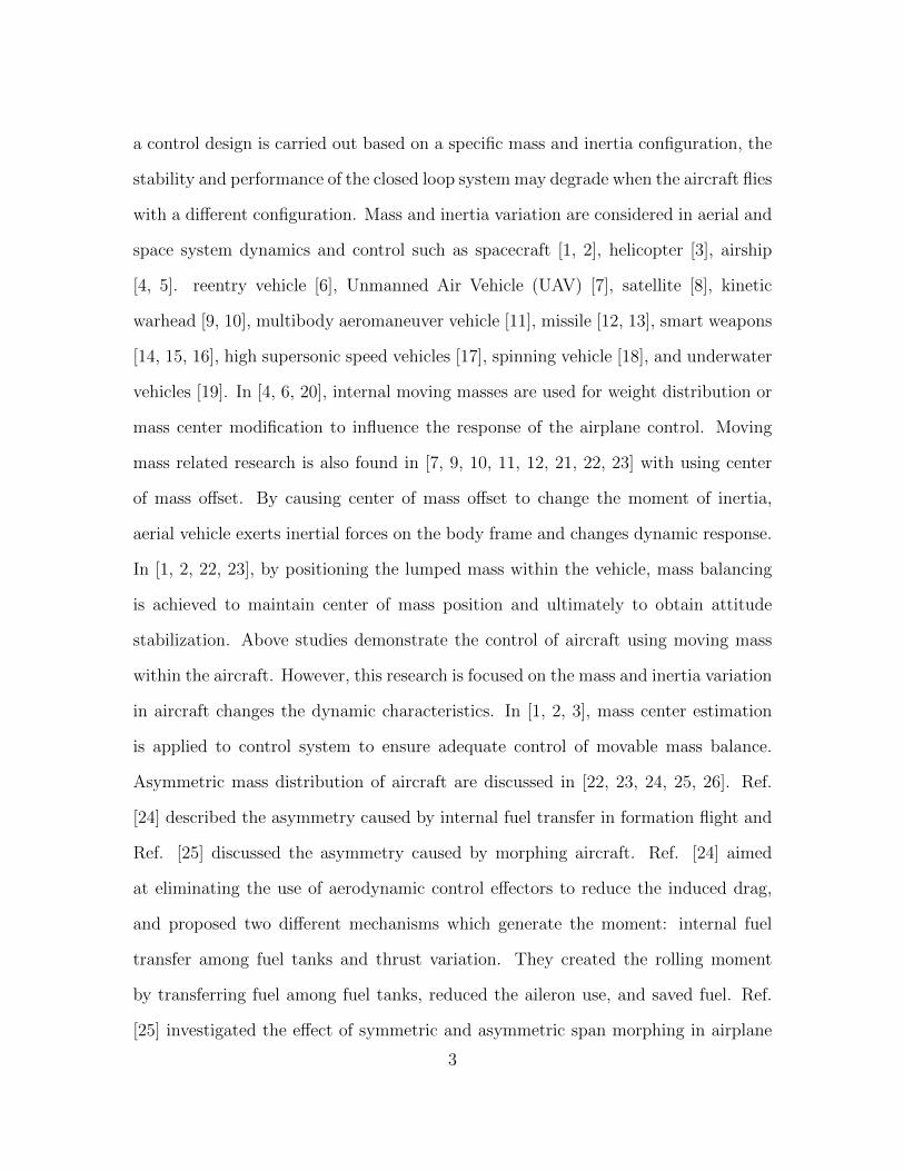
with a different configuration. Mass and inertia variation are considered in aerial and
space system dynamics and control such as spacecraft [1, 2], helicopter [3], airship
[4, 5]. reentry vehicle [6], Unmanned Air Vehicle (UAV) [7], satellite [8], kinetic
warhead [9, 10], multibody aeromaneuver vehicle [11], missile [12, 13], smart weapons
[14, 15, 16], high supersonic speed vehicles [17], spinning vehicle [18], and underwater
vehicles [19]. In [4, 6, 20], internal moving masses are used for weight distribution or
mass center modification to influence the response of the airplane control. Moving
mass related research is also found in [7, 9, 10, 11, 12, 21, 22, 23] with using center
of mass offset. By causing center of mass offset to change the moment of inertia,
aerial vehicle exerts inertial forces on the body frame and changes dynamic response.
In [1, 2, 22, 23], by positioning the lumped mass within the vehicle, mass balancing
is achieved to maintain center of mass position and ultimately to obtain attitude
stabilization. Above studies demonstrate the control of aircraft using moving mass
within the aircraft. However, this research is focused on the mass and inertia variation
in aircraft changes the dynamic characteristics. In [1, 2, 3], mass center estimation
is applied to control system to ensure adequate control of movable mass balance.
Asymmetric mass distribution of aircraft are discussed in [22, 23, 24, 25, 26]. Ref.
[24] described the asymmetry caused by internal fuel transfer in formation flight and
Ref. [25] discussed the asymmetry caused by morphing aircraft. Ref. [24] aimed
at eliminating the use of aerodynamic control effectors to reduce the induced drag,
and proposed two different mechanisms which generate the moment: internal fuel
transfer among fuel tanks and thrust variation. They created the rolling moment
by transferring fuel among fuel tanks, reduced the aileron use, and saved fuel. Ref.
[25] investigated the effect of symmetric and asymmetric span morphing in airplane
3

and tested it in an Unmanned Aerial Vehicle (UAV) for a loitering mission. Ref.
[25] indicated that span morphing leads the aerodynamic and structural change, and
these affect the force, moment, and mass properties of the aircraft. Ref. [25] further
stated that flight dynamics and control are affected significantly by these changes.
1.3.2 Gain Scheduling Methods in Aircraft Control
1.3.2.1 Application of Gain Scheduling in Vehicle Control
Gain scheduling control methods are widely used for controlling nonlinear sys-
tems, especially aerospace vehicles. Some examples include the pitch axis of a missile
[27], business jet aircraft control in a longitudinal flight [28], missile autopilot [29],
large flexible Engineering Test Satellite VIII (ETS-VIII) [30], pitch-axis autopilot of
an air-to-air missile [31], automated surface-to-air missile with dynamics influenced
by Mach number and altitude during the flight [32], NASA’s Orion control system
design for launch abort vehicle [33], F-16 aircraft control with detailed aerodynamic
data [34], attitude motion control of the pitch axis dynamics of the X-33 vehicle during
ascent for velocities greater than Mach 2 [35], longitudinal motion of the F-18 air-
craft [36], autopilot design for a missile pitch-channel control [37], longitudinal flight
of Lockheed P2V-7 [38], and unmanned combat air vehicle (UCAV) model of Lock-
heed Martin’s ICE (Innovative Control Effectors) 101-TV [39]. The modern/classical
applications of gain scheduling are listed in [31] as jet engines, active suspensions,
high-speed drives, missile autopilots, and VSTOL aircraft. Other application areas
in addition to aerospace engineering are reel-winding mechanism [40], two-link flex-
ible manipulator system including both rigid body and lightly damped structural
mode [41], nonlinear continuous stirred tank reactor CSTR) chemical process [42]
and three-level voltage-source inverters (VSI) for high power systems [43].
4

1.3.2.2 Types of Gain Scheduling Control Design Methods
Gain scheduling design technique has no strict theoretical basis. When gain
scheduling technique is used as a nonlinear control method, there are two main ap-
proaches of parameterizing linear models: (i) linearization-based method [42, 39, 44,
45, 33, 46, 37] and (ii) linear parameter-varying (LPV) method [27, 30, 35, 36, 38,
40, 41, 45, 46, 47, 28, 31]. In the linearization-based method, the nonlinear model
is approximated, through linearization, by multiple linear time invariant models at
different operating conditions of choice. In LPV method, the nonlinear model is refor-
mulated as a linear time-varying model [31]. As the first step of linearization-based
method, several operating points need to be selected. Generally, these operating
points are chosen from equilibrium points within the operating domain of the original
nonlinear system. For each operating point, a linear controller is designed, which
may require the linearization of the nonlinear model around each operating point.
Then each linear controller is connected and formed into a single nonlinear controller.
Lawrence and Rugh [45] use a family of linear controllers, each of which is designed
based on the linearized plant at each operating point. One of the main requirements
for gain scheduled controllers is that the linearized closed loop system at an operating
point should have exactly the same properties as the linear controller designed for
that operating point. Ref.[46] shows that this linearization property is retained when
the discrete-equivalence of the gain scheduled controller via stop-invariant or bilinear
transformation techniques is implemented in the sampled-data system implementa-
tion. The classical (static) gains are scheduled with variables which parameterize
the equilibrium points through a series of equilibrium linearizations. The parame-
ters can be control inputs or slowly-varying states. Dynamic gain seheduling uses
fast-varying states. Ref. [39] does the dynamic gain scheduling by applying a trans-
5

formation to the classical gain schedules. In LPV method, the plant dynamics is
reformulated to transform nonlinearities to linear time-varying parameters. These
linear time-varying parameters are used as scheduling variables and scheduling is di-
rectly performed with the varying parameters of the system. For LPV system based
gain scheduling [27, 30, 35, 36, 38, 40, 41, 45, 46, 48, 47, 28, 31], there are different
methods to parameterize linear models. The linear models are represented by time-
varying state-space matrices that are functions of varying parameters [30]. For LPV
systems, the parameter variations is assumed to be independent of the system states.
Ref. [35] applies the same method for quasi-LPV systems where the dependency of
the parameter variation on the system states is ignored. In classical gain scheduling,
it is hard to guarantee the global stability of the closed-loop system over the entire
operating domain. The drawbacks of the classical gain scheduling design is found
in both linearization-based method and LPV method. Saussie et al.[28] indicate the
drawbacks of LPV method. According to them, in LPV technique, the controllers
are directly obtained in a LPV format and this form is formulated as Linear Matrix
Inequalities (LMI) optimization problems. They state that, with large operating do-
main, the LPV method cannot guarantee a global stability of the closed loop system
because it is hard to conduct LMI optimization problem and the results show unrealis-
tic answers. The linearization-based method has limitations such that the closed-loop
stability and performance are assured only around the vicinity of the operating points
and the parameter variation cannot be fast. Doyle III et al.[49] indicates that the tra-
ditional gain scheduling design takes fixed scheduling variables, so past values, time,
and future transitions cannot influence the scheduling variables. When the operating
conditions are changed, fixed variables cause the slow variations. Because of these
limitations of classical gain scheduling techniques, modern gain scheduling design
methods have been developed. Several modern techniques were added to improve the
6

LPV method. When an aircraft experiences rapid dynamic changes, the operating
regions also need to be changed rapidly. However, slow variation condition cannot
contain these operation regions in rapid manners [34]. To overcome this difficulty,
dynamic gain scheduling with fast gain is proposed [39, 42, 49, 45]. Jones et al. [39]
state that fast-varying states are ideal parameters for gain scheduling because aircraft
responses are dominated mostly by fast modes and slow modes tend to be damped out
by the pilot or automatic control system. Fast gain in dynamic gain scheduling copes
with rapid changes throughout the range of operating conditions and overcome the
limitation of slow variables. However, hidden coupling terms may appear and cause
instability when fast-varying gain is used. In classical gain scheduling, the parame-
ter is either a control input or a slowly-varying state. In dynamic gain scheduling,
the fast-varying state is used as a parameter and may introduce unwanted additional
dynamics during the partial derivative process in the linearization. Yang et al.[34]
explain that dynamic gain scheduling is a control approach of scheduling controller
gain with at least one fast-varying state associated with hidden coupling terms and
compensating for nonlinearity during rapid maneuvers.
1.3.2.3 Methods to Determine the Number of Operating Points
The number of operating points for the gain scheduling controller requires a
tradeoff between the needs for covering the whole operating domain and for keep-
ing the number smaller to have a simpler controller. To determine the number of
operating points, in Ref. [33], the variation of mass properties, aerodynamics, and
atmosphere with the current nonlinear controller model are considered using Monte
Carlo analysis, then design points are determined based on initial altitude, time, and
Mach number. In Ref. [37], the Mach number and normal acceleration are chosen as
the scheduling variables. The flight envelop is determined based on the limits of the
7

feasible ranges of the Mach number and normal acceleration. The operating points
are determined by dividing the Mach number range into 16 segments and the normal
acceleration range into 67 segments.
1.3.2.4 Selection of Scheduling Variables
To determine scheduling variable, Yoon et al.[27] used fixed parameters of nor-
malized vertical acceleration and pitch rate,McNamara et al.[33] use Mach number,
altitude and time to schedule parameters, and Fujimori et al.[38] use altitude and
flight velocity as gain scheduling parameters. The gain scheduling parameters are
selected from Mach number and angle of attack in controlling pitch angle of a missile
[28]. Theodoulis and Duc [31] use vertical acceleration and Mach number to con-
trol pitch-axis autopilot of an air-air missile. In ref [36], gain scheduling control law
is applied to dynamic equations of motion of F-18 aircraft, thus Mach number and
altitude variations of the longitudinal flight are used for corresponding to different per-
formance specifications. In [37], constant values of commanded normal acceleration
and mach number are chosen as scheduling variables. Gao and Budman [42] consider
four parameters for scheduling gain in PI controller. Shamma and Athans [48] present
analysis for two types of gain scheduled control for nonlinear plant; scheduling on a
reference trajectory and scheduling on the plant output. Stilwell et al. [46] examine
the gain scheduling controller with sampled-data implementation. These sampled
data is obtained from sample period of the controller input, output, and state. In
Ref. [50], angle of attack, roll rate about the velocity vector, and sideslip are selected
as gain scheduling variables to design flight control system for a model of the ICE (In-
novative Control Effector) fighter aircraft. In Ref. [48] studies effect of the selection
of scheduling variables based on reference trajectory versus plant outputs.
8
1.3.2.5 Linear Control Design Methods Used for Each Operating Point
Linear control design methods used for each operating point are proportional
derivative (PD) controller [28, 44], µ-synthesis-based control law and DVDFB (direct
velocity and displacement feedback) control law [30], linear quadratic regulator (LQR)
approach [33], proportional-integral (PI) controllers [42, 51], linear quadratic regulator
and gain scheduling PI controller [43], and state feedback controller [52]. In Ref. [30]
use µ-synthesis-based control law to treat model variation due to paddle rotation
as structured uncertainty of the satellite system, and DVDFB (direct velocity and
displacement feedback) control law to improve tracking performance. In Ref. [31],
proportional-integral/proportional-type controllers are applied to compute the pitch-
axis autopilot of an air-air missile. In Ref. [32], Linear quadratic Gaussian with loop
transfer recovery (LQG/LTR) gain scheduling controller is applied to design surface-
to-air missile autopilot. In [33], once the simplified linear models at each design point
have been created, the PID gain is tuned by using linear quadratic regulator (LQR)
approach. In ref [42], proportional-integral (PI) controllers are used for nonlinear
chemical processes. Alepuz et al. [43] suggest linear quadratic regulator to control
any state variable of the converter in small and large signal operation. They explain
that modeling error and input saturation are explicitly incorporated into the analysis
with gain scheduling PI controller by reformulating a variable gain. For the linear
control design for each operating point in Ref [37], first order transfer functions are
chosen as controller transfer functions. The coefficients of the transfer functions are
parameterized by the gain scheduling variables. Ref. [39] uses LQR-design method
to determine the state-feedback gain while continuation tailoring is used to determine
feed-forward gain schedule to achieve desired steady state behavior. In Ref. [45], an
output feedback and integral-error controller is designed for each operating point to
9
have zero steady-state error. In Ref. [48], each operating point, a finite-dimensional
compensator is assumed to be designed to stabilize the closed loop system.
1.3.2.6 Methods to Construct the Final Nonlinear Form of Gain Scheduling Con-
troller
This section introduces several methods used to put all the linear controllers
together to construct the final nonlinear form of gain scheduling controller. Since LPV
method does not require interpolation process, these are only for the linearization-
based method. Methods used to put all the linear controllers together to construct
the final nonlinear form of gain scheduling controller, Ref. [33] constructs tables
which are based on scheduling variables, tracking gain table and settling gain table,
and gains are interpolated individually for different flight phases. In Ref. [37], the
linear controller coefficients are designed at the boundaries of the design region, and
determined by the upper and lower values of the gain scheduling variables. For
the flight conditions inside the operating region, a second order polynomial of gain
scheduling variables is used to interpolate the gains of the controller. In Ref. [43], the
linear controllers are designed for each operating points corresponding to each design
interval. The final gain scheduling controller consists of the linear controllers with
a switching scheme, which is based on the boundaries between the design intervals.
In Ref. [44], linear controller designed for each operating point is parameterized in
terms of the scheduling variables. This leads to a gain scheduling controller that does
not require interpolation between operating points. In Ref. [42], linear interpolation
function based on four parameters is used to construct the final nonlinear form of
gain scheduling controller. The values of those parameters are determined through
the optimization method.
10

1.3.2.7 Methods to Analyze Stability and Performance Characteristics of the Closed
Loop System
There are two approaches to guarantee the stability and performance of the
closed loop system. One is using control design method [32, 39]. In this case, control
design process guarantees the stability of the system. In Ref.[32], global robust-
ness and performance of the system is guaranteed under parameter-varying condi-
tions by applying time-varying Kalman filter (TVKF). Another is using simulation
models[43, 45, 33, 37, 32]. Once the control design is completed, the closed-loop
system performance at certain flight conditions within the flight envelope is demon-
strated by simulation. In Ref. [32], two different simulations are carried out. In
static simulations, the scheduling variables, Mach number and altitude, are fixed rep-
resenting a specific operating condition, and the closed loop response is obtained to
evaluate the performance of the gain scheduling controller. This simulation experi-
ment is repeated for various values of Mach number and altitude, representing the
four cornets of the flight envelope. In the dynamic simulations, the closed loop per-
formance is demonstrated while the Mach number and altitude are varying according
to defined functions of time. In Ref. [33], the gains are tested and performance
requirements are evaluated in a non-linear simulation using flight software of Orion
vehicle. In Ref. [37], the gain scheduling controller is implemented in a nonlinear
simulation and various simulation cases within the operating ranges are run to show
the performance of the closed loop system. In Ref. [39], the local stability achieved
through LQR design method is expanded globally by using bifurcation diagrams of
the nonlinear system in the continuation-based design method. In Ref. [43], Matlab
and Simulink simulation results are used to validate controller design. In Ref. [44],
the gain scheduling controller is guaranteed to preserve the closed-loop eigenvalues
11
and the input-output relation locally at each operating point. In Ref. [42], to analyze
stability and performance characteristics of the closed loop system, conditions are set
as linear matrix inequalities (LMIs) for nonlinear processes, and LMI-based tests are
derived to analyze and guarantee the closed-loop stability and performance. Also, by
comparing gain-scheduled PI controllers and linear PI controllers, gain-scheduled PI
controllers show better performance.
1.4 Prior Research
In this research, gain scheduling based on mass variation is developed using the
previously developed dynamic model [26] and control method [53]. The mathemati-
cal model of tanker is formulated relative to the inertial frame and the mathematical
model of receiver is derived relative to the tanker aircraft. The separate dynamic mod-
els of tanker and receiver aircraft are implemented in the simulation of the standard
racetrack maneuver in aerial refueling operation. An integrated simulation environ-
ment is developed to take into account tanker maneuvers, motion of the receiver
relative to the tanker and the aerodynamic coupling due to the trailing wake-vortices
of the tanker. The full 6-DOF nonlinear dynamics of the tanker aircraft is used in
simulation. In the receiver’s equations of motion, mathematical quantities contain
the physical parameters of the receiver aircraft, and its fuel tanks and wind effects.
These equations are used in simulation. Equations of motion for the receiver aircraft
have the properties of time-varying mass and inertia associated with fuel transfer,
and the vortex induced wind effect from the tanker. The equations of motion are
implemented in an integrated simulation environment with feedback controllers for
tanker and receiver aircraft. The feedback controller for the receiver is to fly the re-
ceiver aircraft along a desired trajectory defined relative to the tanker. The controller
for the tanker is to fly the aircraft at the commanded altitude, airspeed, and turn
12
rate. Both controllers are designed with LQR-based MIMO state-feedback and inte-
gral control method. The tanker aircraft model represents KC-135R and the receiver
aircraft model is for a tailless fighter aircraft with innovative control effectors (ICE)
and thrust vectoring capability. Thus, the receiver aircraft has six control variables
(three control effectors, throttle setting and two thrust vectoring angles) while the
tanker has four standard control variables (three control surfaces and throttle set-
ting). Since the receiver has redundant control variables, various control allocation
schemes are investigated for trajectory tracking and station-keeping while the tanker
flies in various racetrack maneuvers with different commanded turn rate. Mass and
inertia variation of the receiver aircraft is modeled by point-masses with varying mass
and positions, representing fuel in each of four fuel tanks. Gain scheduling in both re-
ceiver and tanker controllers are performed with scheduling variables of airspeed and
turn rate based on six nominal cases of two different airspeeds and three turn rates
while the mass/inertia properties are assumed to be fixed in control design [26],[53].
1.5 Original Contributions
This research effort focuses on addressing the issue of mass/inertia variation
in aerial refueling and formation flight by expanding the gain scheduling scheme to
include fuel mass in each fuel tank among the scheduling variables in addition to
airspeed and turn rate. The fuel mass in each fuel tank is considered as state variable
in addition to the standard states associated with aircraft dynamics. All possible
fuel distributions, both symmetric and asymmetric, are considered in trim analyses
of the aircraft in straight level and steady-turn flight conditions at constant altitude
and constant airspeed. The gain scheduling controller design requires the definition
of trim conditions in terms of the fuel amounts in fuel tanks for each set of turn
rate and speed. The three turn rates (zero, right turn, and left turn) and two speed
13

values result in six nominal flight conditions, as done with the tanker aircraft. For the
receiver aircraft, the number of mass/inertia configurations to be included in the set
of trim conditions should be determined. The objective is to keep the number of such
fuel tank configurations small while making sure that they will cover the whole span
of the mass/inertia variation of the receiver aircraft. To reduce the number of cases
included in the gain scheduling, similar cases are combined. In each possible case,
the equations of motion are linearized to obtain the state and control matrices. From
the state and control matrices, various transfer functions are computed. Similarity
of the cases are determined based on the eigenvalue locations of the state matrix
and Bode plots of the transfer functions. An LQR-based MIMO (Multi Input Multi
Output) integral control is designed for each nominal flight and mass configuration.
An interpolation scheme based on the ”mass distance” is developed to combine this
linear controllers into the gain scheduling controller. The ”mass distance” is defined
as the norm of the differences between the current fuel tank amounts and those of
each nominal mass configuration. This gain scheduling controller is implemented
in aerial refueling simulation for a tailless delta wing aircraft with thrust vectoring
capability. The receiver controller was tuned in three control allocation cases: (1)
no thrust vectoring; only aerodynamic control effects in use, (2) both aerodynamic
effectors and thrust vectoring in use, and (3) no elevator or rudder used; only thrust
vectoring and aileron in use. The performance of the gain scheduling controller is
evaluated through the aerial refueling maneuver when the receiver moves between
the observation position, point on the side and behind the tanker, and the refueling
position, a point right behind and slightly below the tanker. The simulation results
first of all demonstrates that the a linear controller designed based on a nominal
flight condition and mass configuration cannot safely complete the refueling maneuver
when the aircraft has a different mass configuration. The simulation results further
14
shows that the gain scheduling controller employing mass configuration as additional
scheduling variables can successfully carry out the refueling maneuver with various
symmetric and asymmetric fuel tank configuration.
1.6 Dissertation Organization
This Dissertation is organized as follows. Chapter 2 presents tanker and re-
ceiver aircraft models which include physical parameters, equations of motion, engine
model, and actuator model. Also tanker aircraft’s vortex model and its effect on
the receiver dynamics will be explained in this section. Chapter 3 presents control
design of receiver and tanker models. Requirements, nominal condition analysis and
gain scheduling controller of both aircraft will be introduced. Determinations of the
nominal conditions to be included in gain scheduling controller for receiver aircraft
using eigenvalues and bode plot analysis will be explained. Chapter 4 demonstrates
that the controller that is designed based on a specific mass configuration may not
work when the aircraft flies with a different mass configuration. Chapter 5 presents
the approach taken to expand the gain scheduling to include the mass configuration
of the aircraft. Chapter 6 shows simulation results. Chapter 7 discusses conclusion
and future work.
15

CHAPTER 2
AIRCRAFT MODELS
2.1 Tanker Aircraft
Evaluation of aerial refueling controllers in simulation needs to include full
dynamic models of tanker and receiver aircraft. Generally, tanker aircraft flies in a
pre-specified racetrack maneuver relative to an inertial frame during the standard
aerial refueling operation. The tanker dynamics equations were developed previously
[26] and a matrix form of the equations is presented in this section.
2.1.1 Aircraft Description
This section explains physical parameters of the tanker aircraft. A Boeing KC-
135 model is used as tanker in this research. KC-135 aircraft has maximum take off
weight 322.500 lbs and normal operating weight of 122.500 lbs [54]. KC-135 aircraft
has aerial refueling boom which is located at the end of the tanker fuselage. The
boom is connected at the tanker fuselage with the boom pivot, and this allows yaw
and pitch motion of the boom relative to the fuselage [54]. The extendable portion of
the boom is fully retracted inside the boom and extends up to 20 ft outside the boom
[54]. At the end of the boom, two control surfaces, called ruddevators, are located.
Each of the ruddevator has a 31 in chord and 61 in span, and it is mounted at a 42
deg dihedral angle with one another [54]. The functions of ruddevator are to allow
the boom operator to move the boom toward the receptacle of receiver aircraft, and
to help mitigate loads on the boom and bending during connected flight [54]. The
boom fairing is of elliptical shape to reduce the drag in the free stream direction.
16
The boom can transfer fuel at the rate of up to 2,900 kg/min [54]. When deflected,
the boom is located downward slope of 32.5 degrees relative to the fuselage reference
plane [55].
2.1.2 Equations of Motion
2.1.2.1 Translational Kinematics
The translational kinematics equation is written in terms of the position vector
of the tanker with respect to an inertial frame. Translational kinematics equation of
the tanker aircraft in matrix form is
rBT = RTBTIRBTWT
VωT + W (2.1)
where rBT is the position of the tanker relative to the inertial frame expressed in the
inertial frame, RBTI is the rotation matrix from the inertial frame to the body frame
of the tanker, RBTWTis the rotation matrix from the tanker wind frame to body
frame of the tanker, and VωT is the velocity of the tanker relative to the surrounding
air expressed in the wind frame of the tanker. Additionally, the vector W is the
representation of the local wind velocity in the inertial frame, expanded as
W =
Wx
Wy
Wx
(2.2)
In addition to the matrix forms, the scalar forms of translational kinematics equations
are
xT =VT[
cos βT cosαT cos θT cosψT + sin βT (− cosφT sinψT + sinφT sin θT cosψT )
+ cos βT sinαT (sinφT sinψT + cosφT sin θT cosψT )]
+Wx (2.3)
17
yT =VT[
cos βT cosαT cos θT sinψT + sin βT (cosφT cosψT + sinφT sin θT cosψT )
+ cos βT sinαT (− sinφT cosψT + cosφT sin θT sinψT )]
+Wy (2.4)
zT =VT[− cos βT cosαT sin θT + sin βT sinφT cos θT + cos βT sinαT cosφT cos θT
]+Wz (2.5)
where (xT , yT , zT ) is the position of the tanker aircraft relative the inertial frame,
(ψT , θT , φT ) is the orientation of the tanker relative to the inertial frame in terms of
the Euler angles, (VT , βT , αT ) are the airspeed, side slip angle and angle-of-attack of
the tanker.
2.1.2.2 Translational Dynamics
Translational dynamics equation of the tanker aircraft in matrix form isVωT
βT
αT
= ET−1S(ωBT)RBTWT
VωT + ET−1S(ωBT)W − ET−1W
+1
mT
ET−1(RBTIMT + RBTWTAT + PT ) (2.6)
where
ET−1 =
cosαT cos βT sin βT sinαT cos βT
− 1VωT
cosαT sin βT1
VωTcos βT − 1
VωTsinαT sin βT
− 1VωT
sinαT sec βT 0 1VωT
cosαT sec βT
(2.7)
VωT is the airspeed, βT is sideslip angle, αT is angle-of-attack, mT is the mass of
the tanker, and S(ωBT) is skew-symmetric matrix formed with representation of ωBT .
The three different forces acting on the tanker aircraft are
MT =
0
0
mTg
AT =
−DT
−ST
−LT
PT =
TT cos δT
0
−TT sin δT
(2.8)
18

where MT is the gravitational force expressed in the inertial frame, AT is the aero-
dynamic force expressed in the wind frame of the tanker, PT is the propulsive force
expressed in the body frame of the tanker, and g is the gravitational acceleration.
Also, DT is the drag, ST is side force, LT is lift, TT is the thrust magnitude, and δT
is the thrust inclination angle of the tanker. The scalar forms of the translational
dynamics are
VT = g [cos θT sin βT sinφT + cos βT (cosφT cos θT sinαT − cosαT sin θT )]
+1
mT
[−DT + TT cos (αT + δT ) cos βT ] (2.9)
βT = −rT cosαT + pT sinαT
+g
VT[− cosφT cos θT sinαT sin βT + cos βT cos θT sinφT + cosαT sin βT sin θT ]
− 1
mT VT[ST + TT cos (αT + δT ) sin βT ] (2.10)
αT = qT − (pT cosαT + rT sinαT ) tan βT
+g sec βTVT
[cosαT cosφT cos θT + sinαT sin θT ]
− sec βTmT VT
[LT + TT sin (αT + δT )] (2.11)
where (pT , qT , rT ) is the angular velocity of the tanker expressed in the tanker’s body
frame. The standard expressions of the aerodynamic forces are
DT =1
2ρV 2
T STCDT , (2.12)
ST =1
2ρV 2
T STCST , (2.13)
LT =1
2ρV 2
T STCLT , (2.14)
19
where ST is the reference area of the tanker and ρ is the ambient air density. Also,
the aerodynamic coefficients are
CDT = CD0 + CDα2 α2T (2.15)
CST = CS0 + CSββT + CSδrδrT (2.16)
CLwing = CL0 + CLααT + CLα2 (αT − αref )2 + CLqcT
2VTqT (2.17)
CLtail = CLδeδeT (2.18)
CLT = CLwing + CLtail (2.19)
where (δaT ,δeT ,δrT ) are the deflections of the control surfaces (aileron, elevator, rudder,
respectively) and cT is the chord length for the tanker.
2.1.2.3 Rotational Kinematics
The rotational kinematics equation of the tanker aircraft in matrix form is
RBTIRBTI = −S(ωBT) (2.20)
where ωBT is the angular velocity vector of the tanker relative to the inertial frame
expressed in its own body frame as
ωBT =
pT
qT
rT
(2.21)
The rotational motion of the tanker aircraft in terms of Euler angles is, in scalar form,
φT = pT + qT sinφT tan θT + r cosφT tan θT (2.22)
θT = qT cosφT − r sinφT (2.23)
ψT = (qT sinφT + rT cosφT ) sec θT (2.24)
where note that both the orientation in terms of (ψT , θT , φT ), and the angular velocity.
(pT , qT , rT ), of the tanker are relative to the inertial frame.
20

2.1.2.4 Rotational Dynamics
The rotational dynamics equation of the tanker aircraft in matrix form is
ωBT = It
−1MBT + It
−1S(ωBT)I
tωBT (2.25)
where It
is the inertia matrix of the tanker aircraft. MBT is the moment of the
external forces around the origin of the tanker’s body frame and expressed in the
body frame of the tanker as
MBT =
LT
MT
NT
(2.26)
where LT is rolling moment, MT is pitching moment, and NT is yawing moment of
the tanker. The scalar forms of the rotational dynamics equations are given as:
pT =1
(IxxIzz − I2xz)
[(Ixx − Iyy + Izz)IxzpT qT + (Iyy − Izz + I2zz − I2
xz)qT rT
+IzzLT + IxzNT ] (2.27)
qT =1
Iyy[(Izz − Ixx)pT rT + (r2
T − p2T )Ixz +MT ] (2.28)
rT =1
(IxxIzz − I2xz)
[(I2xx − IxxIyy + I2
xz)pT qT + (−Ixx + Iyy − Izz)IxzqT rT
+IxzLT + IxxNT ] (2.29)
where I(·)(·) is the moment or product of inertia of the tanker relative to the corre-
sponding axis of the tanker’s body frame. Note that the notation for I(·)(·) is the
same for both tanker and the receiver while their values are obviously different. The
rolling, pitching, and yawing moments of the tanker aircraft is,
LT =1
2ρV 2
ωTST bTCLT (2.30)
MT =1
2ρV 2
ωTST cTCMT
+4ZTTT (2.31)
NT =1
2ρV 2
ωTST bTCNT (2.32)
21

where bT is the wingspan of the tanker aircraft and 4ZT is the moment arms of the
thrust in the tanker’s body frame. The aerodynamic moment coefficients are
CLT = CL0 + CLδaδaT + CLδrδrT + CLββT + CLpbT
2VωTpT + CLr
bT2VωT
rT (2.33)
CMT= CMααT + CMδe
δeT + CMq
cT2VωT
qT (2.34)
CNT = CN0 + CN δaδaT + CN δrδrT + CNββT + CNpbT
2VωTpT + CNr
bT2VωT
rT (2.35)
2.1.3 Engine Model
The thrust generated by the engine (TT ) is
TT = ξT TmaxT (2.36)
where ξT denotes the instantaneous throttle setting and TmaxT is the maximum avail-
able thrust of the tanker and assumed to be constant in this paper. The engine
dynamics is modeled as that of a first order system with time constant τT . Therefore,
we have
ξT =ξT − ξtTτT
, (2.37)
where ξtT is the commanded throttle setting (0≤ ξt ≤ 1).
2.1.3.1 Actuator Model
For the present study, only the actuator saturation are considered. The deflec-
tion range attainable from each control surface is within (-20 deg, 20 deg).
2.2 Receiver Aircraft
In an efficient aerial refueling operation, the receiver aircraft needs to be con-
trolled with respect to the tanker’s position and orientation rather than with respect
to the inertial reference frame. Moreover, the receiver aircraft will be exposed to a
nonuniform wind field during the whole refueling operation when it is in the proximity
22

of the tanker due to the trailing vortices of the tanker. Nonlinear equations of receiver
aircraft were derived [26] with respect to the tanker’s position and orientation. Dur-
ing the aerial refueling operation, receiver aircraft moves to the contact position and
stays relative to the tanker while tanker aircraft executes a pre-specified racetrack
maneuver relative to the inertial frame [26], [53]. Matrix forms of the equations are
given in this section as they are used in the simulation of the closed loop system.
2.2.1 Aircraft Description
This section explains the physical parameters of the receiver aircraft. The
Innovative Control Effector (ICE) unmanned aircraft is used as the receiver aircraft
in this research and being fueled from a KC 135 tanker aircraft. ICE aircraft was
developed under a U.S. Air Force Research Laboratories (AFRL) sponsored program
[50]. It is a tailless, single engine, and supersonic fighter aircraft with a 65 degree
sweep delta wing [50]. It has conventional control effectors such as elevons, symmetric
pitch flaps, and outboard leading-edge flaps, and has innovative control effectors which
are pitch and yaw thrust vectoring, all-moving tips, and spoiler slop deflectors [50]. In
ref. [56], vehicle configuration is depicted using the ICE101. Pitch flap is used for
Table 2.1. ICE 101 Configuration and Aerodynamic Data [56]
Reference Wing (Planform) Area 808.58 sq.ftWing Span 37 ft 6.0 in (450.00 in)
Reference Wing Aspect Ratio 1.74Leading Edge Wing Sweep Angle 65.0 degree
Trailing Edge Sweep Angle 25 degreeBody Length (Centerline Chord) 517.49 in
Reference Wing Mean Aerodynamic Chord 335.33 inFuselage Station of Leading Edge of Wing Mean Aerodynamic Chord 165.67 in
23
pitch axis and elevon is used for roll control. Clam shells, which provide symmetrical
deflection of top and bottom of the wing, are used for yaw control and speed brake
function [56]. Some reference dimensions are given in Table 2.1.
2.2.2 Equations of Motion
2.2.2.1 Translational Kinematics
The translational kinematics equation is written in terms of the position vec-
tor of the receiver aircraft with respect to the tanker body frame. Translational
kinematics equation of the receiver aircraft in matrix form is
ξ = RTBRBT
RBRWRU + RT
BRBTW −RBTI rBT + S(ωBT
)ξ (2.38)
where ξ is the position vector of the receiver relative to the tanker expressed in the
body frame of the tanker, U is the velocity of the receiver relative to the surrounding
air expressed in the wind frame of the receiver (WR-Frame), W is the velocity of the
surrounding air relative to the ground expressed in the body frame of the receiver,
and rBT is the velocity vector of the tanker relative to the inertial frame expressed
in the inertial frame. RBRBTis the rotation matrix from tanker’s body frame (BT -
Frame) to receiver’s body frame (BR-Frame), RBRWRis the rotation matrix from
wind frame of the receiver (WR-Frame) to body frame of the receiver (BR-Frame)
and parameterized by the angle of attack (αR) and sideslip angle (βR) of the receiver,
and RBTI is the rotation matrix from the inertial frame to body frame of the tanker
(BT -Frame).
24
2.2.2.2 Translational Dynamics
Translational dynamics of the receiver in matrix form is
XR = E−1R [S(ωBRBT) + S(RBRBT
ωBT)] (RBRWR
U +W )− E−1R W
+1
(M +m)E−1R
[RBRBT
RBTI (F + m rBT )
− m(RBRWR
U +W −RBRBTVm + RT
BRBTS(ωBT
)ρc) ]
− 1
(M +m)E−1R
k∑j=1
(mj
{ρmj − [S(ωBRBT
) + S(RBRBTωBT
)] ρmj
}+ mj
{ρmj + S(ωBRBT
)[S(ωBRBT
)ρmj − 2ρmj]
+ 2S(RBRBTωBT
)[S(ωBRBT
)ρmj − ρmj]
+[S2(RBRBT
ωBT)− S(RBRBT
ωBT)]ρmj + S(ρmj
)ωBRBT
})(2.39)
where
XR =
[VR βR αR
]T(2.40)
U =
VR
0
0
(2.41)
ER =
cos βR cosαR −VR sin βR cosαR −VR cos βR sinαR
sin βR VR cos βR 0
cos βR sinαR −VR sin βR sinαR VR cos βR cosαR
(2.42)
and ωBRBT is the angular velocity vector of the receiver relative to the tanker repre-
sented in body frame of the receiver, ωBT is the angular velocity vector of the tanker
relative to the inertial frame, S(ωBRBT) is skew symmetric matrix constructed with
representation ωBRBT , M is mass of solid part of the receiver, m is total mass of fuel,
F is total external force acting on the receiver aircraft, Vm is velocity of fuel flow into
the receiver aircraft relative to the tanker, mj is mass of fuel in jth fuel tank of the
25

receiver, and ρmj is the position vector of the center of mass of the fuel mass in the
jth tank expressed in body frame of the receiver (BR-Frame).
2.2.2.3 Rotational Kinematics
The standard rotational kinematics equations are used both in tanker and re-
ceiver aircraft. However, their interpretations are different because angular position
and angular velocity of the receiver aircraft are relative to tanker body frame, an
accelerating and rotating reference frame. The rotational kinematics equations of the
receiver aircraft in matrix form take the form of Poisson’s equation as
RBRBT= S(ωBRBT
)RBRBT(2.43)
where ωBRBT is the representation of the angular velocity vector of the receiver aircraft
relative to the tanker body frame expressed in its own body frame as
ωBRBT =
pRT
qRT
rRT
(2.44)
The scalar form of this matrix equation in terms of Euler angles are
φ = p+ q sinφ tan θ + r cosφ tan θ (2.45)
θ = q cosφ− r sinφ (2.46)
ψ = (q sinφ+ r cosφ) sec θ (2.47)
where note that both the orientation, (ψ, θ, φ), and the angular velocity, (p, q, r), of
the receiver are relative to the tanker.
26

2.2.2.4 Rotational Dynamics Equation
The rotational dynamics equation of the receiver aircraft in matrix form is
ωBRBT = I−1tMBR + I−1
tS(ωBRBT
+ RBRBTωBT
)IM
(ωBRBT + RBRBTωBT )
+ I−1t
k∑j=1
S(ρmj)[mj
(ωTBRBT + ωTBTR
TBRBT
)ρmj (ωBRBT + RBRBT
ωBT )
+mj ρmj + mj ρmj
]+ I−1
t
[k∑j=1
S(ρmj) mj
] {− [S(ωBRBT
) + S(RBRBTωBT
)] (RBRWRU +W )
+ER XR + W}
+ I−1t
[S(ρmj
) mj
](RBRwR
U +W )
− 2 I−1t
k∑j=1
mj
[(ρTmj ρmj
)I3×3 − ρmjρTmj
](ωBRBT + RBRBT
ωBT )
− I−1t
k∑j=1
mj
[(ρTmj ρmj
)I3×3 − ρmjρTmj
](ωBRBT + RBRBT
ωBT )
− S(ωBRBT) RBRBT
ωBT −RBRBTωBT
− It
−1mS(ρR) (RBRBTRBTIrBT + RBRBT
Vm −RBRBTS(ωBT )ρc) (2.48)
where It
is the total inertia matrix of the entire system (receiver and fuel) at a given
time in body frame of the receiver (BR-Frame), always non-singular, and IM
is the
inertia matrix of the receiver, excluding fuel transferred. MBR is the total moment of
the external forces acting on the receiver due to the source of gravity, aerodynamics,
and propulsion about the origin of body frame of the receiver. In Eq. (2.48), only
rBT (the velocity of the tanker relative to the inertial frame) is with respect to the
inertial frame. Other representations are in either body frame of tanker or in body
frame of receiver aircraft. In rotational dynamics, refueling effect is represented by
the concentrated fuel mass and its center of mass location in each fuel tank. In
present work, receiver airplane has four fuel tanks and the effect of fuel flow into each
27

tank is taken into account separately. A center of mass change during refueling is
incorporated in the equation by writing the equation with respect to a point fixed
geometrically in the BR-frame. Similarly, aerodynamic variables such as airspeed,
angle of attack, side-slip angle, and aerodynamic stability derivatives are determined
by the geometric shape of the aircraft, and thus standard definitions can be applied
directly without modification [26].
2.2.3 Engine Model
As in the case of the tanker, the engine model ofthe receiver is also a first order
transfer function with constant maximum thrust, obviously with different maximum
thrust and different time constant.
2.2.4 Actuator Model
For the present study, only the actuator saturation and rate limit effects are
considered for the receiver. The deflection range attainable from the elevon is (-30
deg, 30 deg), from the pitch flap (-30 deg, 30 deg) and from the clamshells (-60 deg,
60 deg). All three control effectors have a rate limit of ±90 deg/sec. Likewise, the
thrust vectoring has a limit of ± 30 deg in both directions and a rate limit of ±30
deg/sec.
2.2.4.1 Fuel Tank Configuration
This section describes how the receiver aircraft’s fuel tanks are incorporated
with mathematical quantities in the equations of motion. Fig. 2.1 depicts the fuel
tanks and control surfaces of ICE aircraft. ICE aircraft has four different fuel tanks
symmetrically located with respect to xz-plane. During fuel transfer in standard aerial
refueling operation, the fuel flown into the receiver is equally distributed among the
28

Figure 2.1. Receiver aircraft with its fuel tanks [26].
four fuel tanks. In the ICE receiver aircraft, 35% of fuel capacity is from the front
tanks, tank 1 and tank 2. 65% of fuel capacity is from the tank 3 and tank 4. The
overall fuel flow rate (m) from the tanker to the receiver aircraft is considered as an
external input. The actual mass contained in the jth fuel tank at any instance of time
is computed by integrating fuel flow rate for jth fuel tank (mj) over time. The fuel
mass amount in the jth fuel tank at any instant of time is formulated as
mj(t) =
∫ t
0
mj(τ)dτ (2.49)
where t is time. In case of any residual fuel remains in the tank before the refueling
started, the residual fuel is considered as part of the receiver aircraft. Therefore, when
the refueling is not yet conducted, mj(0) = 0. The position vector of the fuel mass
concentrated at the jth point is denoted by ρmj
, and expressed in BR-frame. Note
that it is assumed that all fuel tanks are rectangular shape, fuel remains level within
29
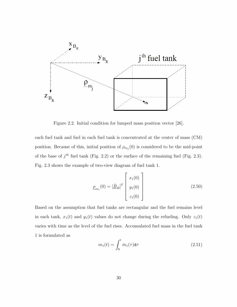
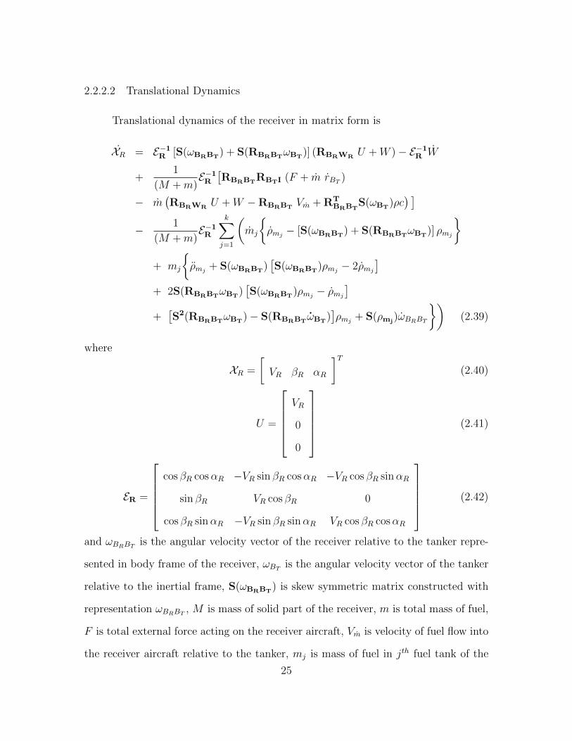
Figure 2.2. Initial condition for lumped mass position vector [26].
each fuel tank and fuel in each fuel tank is concentrated at the center of mass (CM)
position. Because of this, initial position of ρmj(0) is considered to be the mid-point
of the base of jth fuel tank (Fig. 2.2) or the surface of the remaining fuel (Fig. 2.3).
Fig. 2.3 shows the example of two-view diagram of fuel tank 1.
ρm1
(0) = [BR]T
x1(0)
y1(0)
z1(0)
(2.50)
Based on the assumption that fuel tanks are rectangular and the fuel remains level
in each tank, x1(t) and y1(t) values do not change during the refueling. Only z1(t)
varies with time as the level of the fuel rises. Accumulated fuel mass in the fuel tank
1 is formulated as
m1(t) =
∫ t
0
m1(τ)dτ (2.51)
30
Figure 2.3. Two-view diagram of fuel tank 1 [26].
where m1(t) is the fuel flow rate into tank 1. The fuel’s height of the CM from the
base of the fuel tank as fuel is flowing in is calculated as
h1(t) =m1(t)
ρfuela1b1
(2.52)
where a1 is the length, b1 is the breadth of fuel tanks 1, and ρfuel is the density of
the fuel. Time-varying position vector of fuel mass concentrated at the fuel CM in
the fuel tank 1 is
ρm1
(t) = [BR]T
x1(0)
y1(0)
z1(0)− h1(t)2
(2.53)
This time-varying position vector for other fuel tanks are similarly formulated and
the position vectors of all fuel tanks are applied in the receiver’s equations of motion.
31
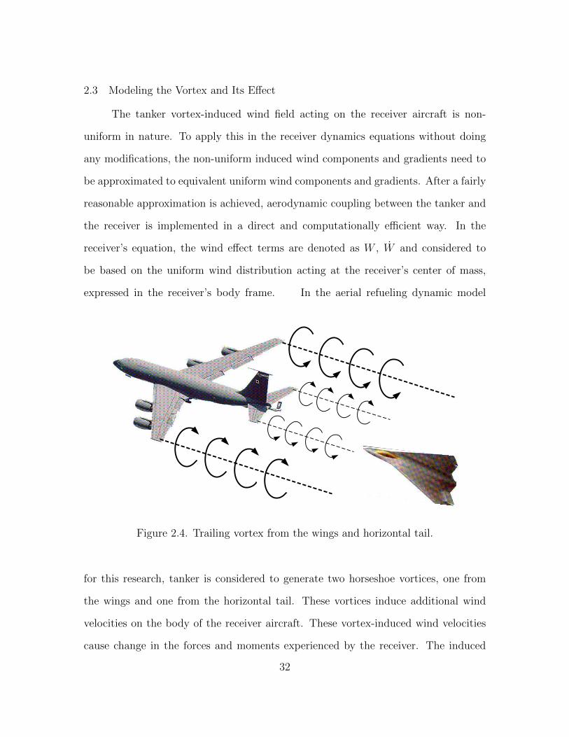
2.3 Modeling the Vortex and Its Effect
The tanker vortex-induced wind field acting on the receiver aircraft is non-
uniform in nature. To apply this in the receiver dynamics equations without doing
any modifications, the non-uniform induced wind components and gradients need to
be approximated to equivalent uniform wind components and gradients. After a fairly
reasonable approximation is achieved, aerodynamic coupling between the tanker and
the receiver is implemented in a direct and computationally efficient way. In the
receiver’s equation, the wind effect terms are denoted as W , W and considered to
be based on the uniform wind distribution acting at the receiver’s center of mass,
expressed in the receiver’s body frame. In the aerial refueling dynamic model
Figure 2.4. Trailing vortex from the wings and horizontal tail.
for this research, tanker is considered to generate two horseshoe vortices, one from
the wings and one from the horizontal tail. These vortices induce additional wind
velocities on the body of the receiver aircraft. These vortex-induced wind velocities
cause change in the forces and moments experienced by the receiver. The induced
32
wind velocities the receiver aircraft experiences are written as a function of the relative
separation as well as the relative orientation between the tanker and the receiver
using a modified horseshoe vortex model based on the Helmholtz profile. Induced
wind and wind gradients are non-uniform along the body dimensions of the receiver
aircraft. Therefore, instead of attempting to directly estimate the induced forces and
moments on the receiver aircraft, the induced wind velocities and wind gradients are
computed by using an averaging technique as uniform approximation. By introducing
the effective wind components and gradients into the nonlinear aircraft equations,
wind components and wind temporal variation of wind in the body frame of receiver
aircraft are used to determine the effects on the receiver’s dynamics. Besides the
actual vortex model and the averaging technique, this model has the effect of vortex
decay over time, different geometrical dimensions for the tanker and the receiver
aircraft, and many useful geometrical parameters of the aircraft such as the wing
sweep angle, the dihedral angle, and the relative distance between the center of mass
of the UAV and the aerodynamic center of the wing.
33

CHAPTER 3
CONTROL DESIGN
3.1 Tanker Aircraft
In an aerial refueling operation, the tanker aircraft flies in a pre-specified course
while a receiver aircraft is refueled, and other receiver aircraft fly in formation waiting
for their turn for refueling. Generally, the tanker aircraft flies at a constant altitude
with a constant speed. The refueling flight course for the tanker aircraft is composed of
steady straight level flight and steady constant altitude turns, and those two combined
flights generate a ”racetrack” maneuver.
3.1.1 Requirements
Even though tanker aircraft in aerial refueling is flown by a human pilot, in
computer simulation, a controller for the tanker aircraft should be designed and im-
plemented to fly any desired racetrack maneuver. In this work, steady turns are
specified by yaw rates of the aircraft. The tanker aircraft is required to satisfy com-
manded yaw rates with small transient and zero steady-state error. While starting
and ending a turn, and during the turn, deviation in altitude and speed from their
respective nominal values should be small and decay to zero at steady-state. In the
simulation environment, the closed-loop performance of the tanker aircraft should be
similar to the flight of manned tanker aircraft in an actual racetrack maneuver.
34

3.1.2 Flight Cases Analysis
Specification of the flight cases and the solution of the equations of motion for
determining the flight cases values of the tanker aircraft states and control variables
at each flight case condition are presented in this section. The trimmed steady-state
flight case varies with the parameterized values of VT0 and ψT0. During the entire
racetrack maneuver, desired side slip is zero (βT0 = 0), airspeed, angle-of-attack,
and altitude are constants (VT = VT0, αT = αT0 and zT0 = 0). For a given steady-
state flight condition whether it is a straight-level or turning flight, angular velocity
components are constants (pT = pT0, qT = qT0 and rT = rT0), pitch and roll angles are
constants (θT = θT0 and φT = φT0), and ψT = ψT0. Then the rotational kinematics
equations at any nominal conditions yield
pT0 = − sin θT0 ψT0 (3.1)
qT0 = sinφT0 cos θT0 ψT0 (3.2)
rT0 = cosφT0 cos θT0 ψT0 (3.3)
Three steady-state trimmed flight conditions yield from the translational dynamics
equations.
0 = g(
cosφT0 cos θT0 sinαT0 − cosαT0 sin θT0
)+
1
mT
[− 1
2ρV 2
T0ST (CD0
+CDααT0 + CDα2α2T0 + CDδeδeT0
) + TT0 cos(αT0 + δT )]
(3.4)
0 = cosφT0 cos θT0 cosαT0ψT0 + sin θT0 sinαT0ψT0 −g
VT0
cos θT0 sinφT0
+1
2mT
ρVT0ST (CS0 + CSδrδrT0+ CSδaδaT0
) (3.5)
0 = sinφT0 cos θT0ψT0 +g
VT0
(cosαT0 cosφT0 cos θT0 + sinαT0 sin θT0)
− 1
2mT
ρVT0ST (CL0 + CLααT0 + CLα2(αT0 − α2ref )
+CLqc
2VT0
sinφT0 cos θT0ψT0 + CLδeδeT0)− 1
mTVT0
TT0 sin(αT0 + δT )(3.6)
35
Other three steady-state trimmed flight conditions yield from the rotational dynamics
equations and the constitutive equations.
0 =1
IxxIzz − I2xz
[− Ixz(Ixx − Iyy + Izz) sin θT0 cos θT0 sinφT0ψ
2T0
+(IyyIzz − I2zz − I2
xz) sinφT0 cosφT0 cos θ2T0ψ
2T0
+1
2ρV 2
T0ST bT Izz(CL0 + CLδaδaT0+ CLδrδrT0
− CLpbT
2VT0
sin θT0ψT0
+CLrbT
2VT0
cosφT0 cos θT0ψT0)
+1
2ρV 2
T0ST bT Ixz(CN0 + CN δaδaT0+ CN δrδrT0
− CNpbT
2VT0
sin θT0ψT0
+CNrbT
2VT0
cosφT0 cos θT0ψT0)]
(3.7)
0 =1
Iyy
[(Ixx − Izz) sin θT0 cos θT0 cosφT0ψ
2T0 + Ixz cos θ2
T0ψ2T0(cosφ2
T0 − 1)
+1
2ρV 2
T0S2T0c(CM0 + CMααT0 + CMδeδeT0
+ CMq
c
2VT0
sinφT0 cos θT0ψT0)
+∆zTTT0 cos δT + ∆xTTT0 sin δT]
(3.8)
0 =1
IxxIzz − I2xz
[− (I2
xx − IxxIyy + I2xz) sin θT0 cos θT0 sinφT0ψ
2T0
+Ixz(−Ixx + Iyy − Izz) sinφT0 cosφT0 cos θ2T0ψ
2T0
+1
2ρV 2
T0ST bT Ixz(CL0 + CLδaδaT0+ CLδrδrT0
− CLpbT
2VT0
sin θT0ψT0
+CLrbT
2VT0
cosφT0 cos θT0ψT0)
+1
2ρV 2
T0ST bT Ixx(CN0 + CN δaδaT0+ CN δrδrT0
− CNpbT
2VT0
sin θT0ψT0
+CNrbT
2VT0
cosφT0 cos θT0ψT0)]
(3.9)
Additionally, since altitude is constant, zT equation in Eq.( 2.5) at a steady-state
trimmed flight condition yields
0 = sinαT0 cosφT0 cos θT0 − cosαT0 sin θT0 (3.10)
Note that in these seven algebraic equations, there are seven unknowns: αT0, θT0,
φT0, TT0, δaT0, δeT0
, δrT0. By solving these seven equations, the nominal values of the
36

unknowns are computed. Further, using Eqs. (3.1), (3.2), and (3.3), the nominal
values of the angular velocity components, pT0, qT0 and rT0, are calculated. Note that
this flight case analysis is parameterized by ψT0. Therefore, when a straight-level
flight is to be analyzed, ψT0 is set to 0. If a specific turn is to be analyzed, then ψT0
is set to the desired turn rate.
3.1.3 Gain Scheduling Controller
A multi-input-multi-output state-feedback LQR and integral control technique
are combined to design controller which is to maintain altitude and speed, and to track
yaw rates. The control variables available for the tanker aircraft are three conventional
control surfaces and throttle setting. The outputs to be controlled are the airspeed,
altitude, and yaw rates. A gain scheduling scheme is implemented based on the
commanded speed and yaw rates. The tanker’s equations of motion which are given
in the previous section are linearized at six different steady-state trimmed nominal
conditions. Two of the nominal conditions correspond to the tanker flying straight
level at constant altitude with two different airspeeds. Other two correspond to the
tanker turning with a specified turn rate to positive direction at constant altitude
with two different airspeeds. And the other two correspond to tanker turning with
a specified turn rate to negative direction at constant altitude with two different
airspeeds. These six flight cases are summarized in Table 3.1. Note that the
flight cses are parameterized by the tanker yaw rates and airspeed. Thus, the flight
case values of the states and the control variables are also functions of the three
parameters. Once a set of flight case values for each of six nominal conditions are
determined, the equations of motion of the tanker are linearized at each flight case
using the respective set of flight case values.
37
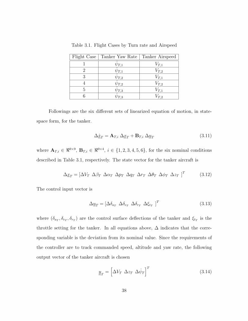
Table 3.1. Flight Cases by Turn rate and Airspeed
Flight Case Tanker Yaw Rate Tanker Airspeed
1 ψT,1 VT,12 ψT,1 VT,23 ψT,2 VT,14 ψT,2 VT,25 ψT,3 VT,16 ψT,3 VT,2
Followings are the six different sets of linearized equation of motion, in state-
space form, for the tanker.
∆xT = AT,i ∆xT + BT,i ∆uT (3.11)
where AT,i ∈ <9×9, BT,i ∈ <9×4, i ∈ {1, 2, 3, 4, 5, 6}, for the six nominal conditions
described in Table 3.1, respectively. The state vector for the tanker aircraft is
∆xT = [∆VT ∆βT ∆αT ∆pT ∆qT ∆rT ∆θT ∆φT ∆zT ]T (3.12)
The control input vector is
∆uT = [∆δaT ∆δeT ∆δrT ∆ξtT ]T (3.13)
where (δaT , δeT , δrT ) are the control surface deflections of the tanker and ξtT is the
throttle setting for the tanker. In all equations above, ∆ indicates that the corre-
sponding variable is the deviation from its nominal value. Since the requirements of
the controller are to track commanded speed, altitude and yaw rate, the following
output vector of the tanker aircraft is chosen
yT
=[∆VT ∆zT ∆ψT
]T(3.14)
38
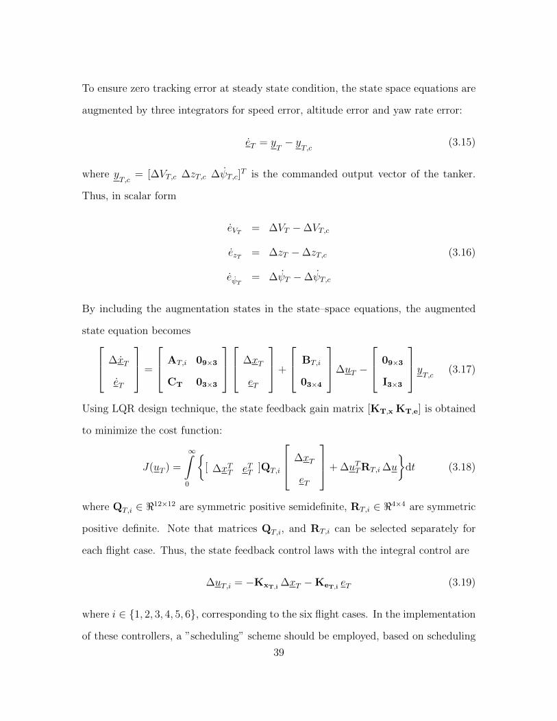
To ensure zero tracking error at steady state condition, the state space equations are
augmented by three integrators for speed error, altitude error and yaw rate error:
eT = yT− y
T,c(3.15)
where yT,c
= [∆VT,c ∆zT,c ∆ψT,c]T is the commanded output vector of the tanker.
Thus, in scalar form
eVT = ∆VT −∆VT,c
ezT = ∆zT −∆zT,c (3.16)
eψT = ∆ψT −∆ψT,c
By including the augmentation states in the state–space equations, the augmented
state equation becomes ∆xT
eT
=
AT,i 09×3
CT 03×3
∆xT
eT
+
BT,i
03×4
∆uT −
09×3
I3×3
yT,c
(3.17)
Using LQR design technique, the state feedback gain matrix [KT,x KT,e] is obtained
to minimize the cost function:
J(uT ) =
∞∫0
{[ ∆xTT eTT ]QT,i
∆xT
eT
+ ∆uTTRT,i ∆u
}dt (3.18)
where QT,i ∈ <12×12 are symmetric positive semidefinite, RT,i ∈ <4×4 are symmetric
positive definite. Note that matrices QT,i, and RT,i can be selected separately for
each flight case. Thus, the state feedback control laws with the integral control are
∆uT,i = −KxT,i∆xT −KeT,i eT (3.19)
where i ∈ {1, 2, 3, 4, 5, 6}, corresponding to the six flight cases. In the implementation
of these controllers, a ”scheduling” scheme should be employed, based on scheduling
39

parameters, ψT and VT to determine effective values of the gains at a given flight
condition. To formulate the overall non-linear controller based on the linear designs
at the six flight cases, Lagrange interpolation scheme is utilized. Thus, the gain
scheduling control law is
∆u =
(ψT,c − ψT,2
)(ψT,c − ψT,3
)(VT,c − VT,2)(
ψT,1 − ψT,2)(
ψT,1 − ψT,3)
(VT,1 − VT,2)u1
+
(ψT,c − ψT,2
)(ψT,c − ψT,3
)(VT,c − VT,1)(
ψT,1 − ψT,2)(
ψT,1 − ψT,3)
(VT,2 − VT,1)u2
+
(ψT,c − ψT,1
)(ψT,c − ψT,3
)(VT,c − VT,2)(
ψT,2 − ψT,1)(
ψT,2 − ψT,3)
(VT,1 − VT,2)u3
+
(ψT,c − ψT,1
)(ψT,c − ψT,3
)(VT,c − VT,1)(
ψT,2 − ψT,1)(
ψT,2 − ψT,3)
(VT,2 − VT,1)u4
+
(ψT,c − ψT,1
)(ψT,c − ψT,2
)(VT,c − VT,2)(
ψT,3 − ψT,1)(
ψT,3 − ψT,2)
(VT,1 − VT,2)u5
+
(ψT,c − ψT,1
)(ψT,c − ψT,2
)(VT,c − VT,1)(
ψT,3 − ψT,1)(
ψT,3 − ψT,2)
(VT,2 − VT,1)u6 (3.20)
Note that the control law assumes the availability of full state measurement or estima-
tion for feedback. The control variables available for the tanker aircraft are the three
conventional control surfaces and the throttle setting. The outputs to be controlled
are the airspeed, altitude and yaw rate.
3.2 Receiver Aircraft
To successfully perform an aerial refueling operation, the receiver is required to
approach to the tanker, stay at the refueling contact position during the actual fuel
transfer, and fly away when the refueling is completed. These three phases should be
40

conducted in a safe manner despite various sources of disturbances such as trail wake
vortex, fuel transfer effect, and motion of the tanker. The receiver aircraft motion is
defined in the tanker’s body frame, thus the reference trajectory for the receiver can
simply be defined relative to the tanker simply. When the receiver is in the station-
keeping phase, that is, receiver needs to be stay at the refueling contact position,
the reference trajectory for the receiver aircraft becomes a point in the body-frame
of the tanker. The receiver’s trajectory-tracking controller is built to follow the safe
reference trajectory in time after ensuring the trajectory from the observation position
to the contact position, and from the contact position to the fly-away path. For the
receiver aircraft, controller is strongly required to fly close to the reference trajectory.
3.2.1 Requirements
The primary requirement of the control design is the tracking of the generated
trajectories, with zero steady-state error in the x, y, z coordinates in the tanker’s body
frame, under the disturbance of trailing vortex, time variation of the inertia prop-
erties of the receiver and the possible steady maneuvers of the tanker’s body frame.
Meanwhile, the control inputs generated by the controller should not cause significant
saturation on the magnitudes and rates of the actuators. Moreover, during the tran-
sient, overshoot or undershoot on trajectory response should be minimized to ensure
the safety of the refueling. At the same time, the response of the closed loop system
should be fast enough so that the approach and fly–away maneuvers are completed
as planned and the high-wind regions of the trailing vortex field are exited in a timely
fashion. Additionally, during the approach, fly–away and station-keeping maneuvers,
the angle-of-attack and the airspeed should not be close to their corresponding stall
values. In this regard, very big pitch angle should not be commanded. Finally, to
ensure the safety of the aircraft, the bank angle should be small relative to its nomi-
41

nal value. As stated earlier, the controller should perform satisfactorily in all phases
of the ”racetrack” maneuver, i.e. while the tanker is in a straight wing-level flight,
in a steady turn, in transition from straight flight to turn and in transition back to
straight flight. Control design of the receiver aircraft should also consider the mass
and inertia variations. That is, the gain scheduling scheme should include mass and
inertia variation of the aircraft due to the change in fuel amounts in all fuel tanks,
and should cover all possible combinations of fuel levels in fuel tanks.
3.2.2 Nominal Condition Analysis
In aerial refueling operation, the receiver aircraft is required to maintain its
position and orientation relative to the tanker aircraft. As in the case of tanker, wind
terms are ignored in the trim analysis and lumbarization. Since the objective of the
receiver is to maintain relative position and orientation with respect to the tanker,
translational and angular velocity components of the receiver should be the same as
those of the tanker. Thus, for nominal condition analysis; V0 = VT0, p0 = pT0, q0 = qT0
and r0 = rT0. Also yaw rates of the tanker and the receiver should be the same
(ψ0 = ψT0). Similar to the tanker, side slip angle of the receiver at the nominal
condition is set to zero (β0 = 0) and the receiver maintain its altitude (z0 = 0). At
nominal condition, the thrust vectoring angles are preferred to be zero (δy0 = 0 and
δz0 = 0). While the dynamic equations of motion of the receiver are written relative
to the tanker as given in Eps. (3.30) and (2.48), for the trim analysis, the equations
relative to the inertial frame are used. Further, at the steady-state, the mass and
42
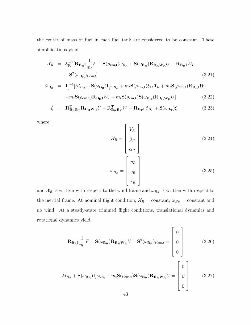
the center of mass of fuel in each fuel tank are considered to be constant. These
simplifications yield
XR = E−1R [RBRI1
mt
F − S(ρcm,t)ωBR + S(ωBR)RBRWR
U −RBRIWI
−S2(ωBR)ρcm,t] (3.21)
ωBR = It
−1[MBR + S(ωBR)I
tωBR +mtS(ρcm,t)ERXR +mtS(ρcm,t)RBRIWI
−mtS(ρcm,t)RBRIWI −mtS(ρcm,t)S(ωBR)RBRWR
U ] (3.22)
ξ = RTBRBT
RBRWRU + RT
BRBTW −RBTI rBT + S(ωBT
)ξ (3.23)
where
XR =
VR
βR
αR
(3.24)
ωBR =
pR
qR
rR
(3.25)
and XR is written with respect to the wind frame and ωBR is written with respect to
the inertial frame. At nominal flight condition, XR = constant, ωBR = constant and
no wind. At a steady-state trimmed flight conditions, translational dynamics and
rotational dynamics yield
RBRI1
mt
F + S(ωBR)RBRWR
U − S2(ωBR)ρcm,t =
0
0
0
(3.26)
MBR + S(ωBR)I
tωBR −mtS(ρcm,t)S(ωBR
)RBRWRU =
0
0
0
(3.27)
43

Since altitude is constant, z equation from translational kinematics yield
z = −VR cosα cos β sin θ + VR sin β sinφ cos θ + VR sinα cos β cosφ cos θ (3.28)
Note that in these seven equations, there are seven unknowns. By solving these seven
equations, the nominal values of the unknowns are computed. Recall that in the
equations of motion of the receiver aircraft, euler angles are relative to the tanker.
While all the other nominal values are directly computed, the relative euler angles
need to be computed.
3.2.3 Linearization
e o ∆y
C u y
0
e
x 0
Tanker ManeuverVortex
∆ x
u
x1s
IntegratorKx
CKe A/C
Figure 3.1. State feedback and integral control structure.
As stated earlier, the gain scheduling controller for the receiver should include
the variation of mass/inertia of the aircraft. This can be done by using the amount
of fuel in each fuel tanks as scheduling parameters in additions to the turn rate and
speed of the aircraft. The gain scheduling controller design requires the definition
of trim conditions in terms of the fuel amounts in fuel tanks for each set of turn
rate and speed. The three turn rates (zero, right turn and left turn) and two speed
values result in six flight cases, as done with the tanker aircraft. For the receiver
aircraft, the number of mass/inertia configurations to be included in the set of trim
44

Table 3.2. Nominal Conditions by Four Receiver Fuel Tanks
Nominal Condition Fuel Filled Tanks
1 None2 Tank4
3 Tank3
4 Tank4, Tank3
5 Tank2
6 Tank4, Tank2
7 Tank3, Tank2
8 Tank4, Tank3, Tank2
9 Tank1
10 Tank4, Tank1
11 Tank3, Tank1
12 Tank4, Tank3, Tank1
13 Tank2, Tank1
14 Tank4, Tank2, Tank1
15 Tank3, Tank2, Tank1
16 Tank1, Tank2, Tank3, Tank4
Figure 3.2. Loci of the eigenvalues as the amount of fuel changes in tank 2, 3, and 4,and tank 1 is empty in cruise condition.
45

Figure 3.3. Zoomed loci of the eigenvalues as the amount of fuel changes in tank 2,3, and 4, and tank 1 is empty in cruise condition.
Figure 3.4. Loci of the eigenvalues as the amount of fuel changes in tanks 1, 3, and4, and tank 2 is empty in steady turn.
conditions should be determined. The objective is to keep the number of such fuel
tank configurations small while making sure that they will cover the whole span of
46

Figure 3.5. Zoomed loci of the eigenvalues as the amount of fuel changes in tanks 1,3, and 4, and tank 2 is empty in steady turn.
Figure 3.6. Loci of the eigenvalues as the amount of fuel changes in all tanks in cruise.
the mass/inertia variation of the receiver aircraft. The ICE receiver aircraft has four
fuel tanks. For each fuel tank, initially five different mass amounts considered are
0%, 25%, 50%, 75%, and 100% full. This leads to 54 = 625 permutations for the four
47

Figure 3.7. Zoomed loci of the eigenvalues as the amount of fuel changes in all tanksin cruise.
Figure 3.8. Bode plot for case-56.
fuel tanks in each of the 6 flight cases. This is obviously too many trim conditions for
a gain scheduling controller. Two different analyses are carried out to determine how
many of these permutations need to be kept and how many can be excluded from
48

Figure 3.9. Bode plot for case-12.
Figure 3.10. Bode plot for case-64.
the gain scheduling controller design: (1) Eigenvalue analysis, and (2) Frequency
domain analysis. In each fuel tank permutation at each nominal flight condition, the
trim analysis and linearization are carried out and the matrices of the state space
representation are constructed. In the eigenvalue analysis, eigenvalues of the open
49

loop state space model are placed on complex domain. If the eigenvalues of multiple
permutations are within a specified proximity, then, all these permutations will be
represented by one of the permutations within the group. In the case of frequency
domain analysis, Bode plots of the open loop system based on the state space matrices
are compared and again the permutations with Bode plots ”close to each other” are
represented by one permutations within the group. This approaches are justified
by the fact that linear systems with eigenvalues or Bode plots close to each other
have similar dynamic characteristics. Through eigenvalue and Bode analyses, it is
demonstrated that, in all six flight cases, fuel tank permutation with 0%, 25%, and
50% full fuel tanks have similar dynamic responses. Similarly, fuel tank permutations
with 75% and 100% fuel have similar dynamical responses. Thus, only 0% and 100%
fuel cases are included in fuel tank permutations considered for gain scheduling control
design. For example, three fuel tanks, 2, 3, and 4, are filled at various levels and tank
1 is empty while the aircraft is in a cruise condition with airspeed VT,2. The eigenvalue
locations of the state matrix of the linearized model at each of the trim conditions
are plotted on the complex domain, as shown in Fig. 3.2. The plot clearly shows that
the eigenvalues of the open loop system moves on the complex domain as the fuel
amount changes in the three fuel tanks. The question here is whether the changes
in the eigenvalue locations are significant to require considerations of all these trim
conditions in the gain scheduling controller. Note that most clusters of eigenvalues
show small movement as the fuel amount changes except the eigenvalues scattered
around -2.0 to -0.7 on or close to the real axis. Fig. 3.3 shows the details about
Fig. 3.2 around the clusters near the intersection between real and imaginary axis.
When the tanks are 100% full, the eigenvalues are complex while in the three other
cases, eigenvalues break into the real axis. Similar trend is seen in Fig. 3.4 and
Fig. 3.5 when eigenvalue locations are analyzed when fuel tanks 1, 3, and 4 are filled
50

at different levels and tank 2 is empty while the aircraft is in a steady-state turn.
Another example, as shown in Fig. 3.6 and Fig. 3.7, is when all fuel tanks are filled
at various levels in a cruise condition. Fig. 3.8 and Fig. 3.2 are in the same condition
such as most deviated cases for the cruise condition. Fig. 3.9 and Fig. 3.4 are in the
condition of most deviated cases for the steady turn. Fig. 3.10 and Fig. 3.6 show
the condition of all four fuel tanks are fully filled in a cruise condition. In Fig. 3.8,
Fig. 3.9 and Fig. 3.10, frequency domain has 4 categories for control input values as
in Eq. (3.31). However in this analysis ∆δy and ∆δz are not considered because these
values are set to be zero at the trim analysis. So only four values are showing in these
figures such as ∆δa, ∆δe, ∆δr, and ∆ξ. In the figure magnitude and phase angle have
three outputs. These three represent output vector in Eq. (3.33) as in ∆x, ∆y, ∆z.
These analyses show that not all fuel levels at 0%, 25%, 50%, 75%, and 100% need
to be considered in gain scheduling as the dynamics of the linear models are ”close”
according to eigenvalue locations. This reduces the number of permutations from 625
to 16 for each nominal flight condition. These 16 cases are tabulated in Table B.2.
Sixteen mass/inertia configurations for each of the six flight case added up to 96 trim
conditions for the gain scheduling controller. These 96 trim conditions are tabulated
in Table A.1 - Table A.3 in Appendix A. Linearizing the equations of motion at each
of the 96 cases leads to 96 different state space representations.
∆x = Ai ∆x+ Bi ∆u+ Hi ∆w (3.29)
where Ai ∈ <12×12, Bi ∈ <12×6, Hi ∈ <12×6, i ∈ {1, ..., 96}, for the combinations of
the six flight cases described in Table 3.1 and 16 conditions listed in Table B.2. The
state vector is
∆x = [∆V ∆β ∆α ∆p ∆q ∆r ∆ψ ∆θ ∆φ ∆x ∆y ∆z]T (3.30)
51

The control input vector is
∆u = [∆δa ∆δe ∆δr ∆ξ ∆δy ∆δz]T (3.31)
The disturbance vector due to the motion of the tanker is
∆w = [∆VxT ∆VyT ∆VzT ∆pT ∆qT ∆rT ∆pT ∆qT ∆rT ∆ψT ∆θT ∆φT ]T (3.32)
In all equations above, ∆ indicates that the corresponding variable is the perturbation
from its nominal value. Note that, since the nonlinear equations of motion are derived
in terms of the states of the receiver relative to the tanker, in the linearized equations,
the effect of the motion of the tanker on the relative motion is clearly identified by Hi
matrices. However, Hi matrices are not utilized in the control design carried out in
this research. Since the position tracking controller is to be designed for the receiver
relative to the tanker, the outputs to be tracked are (∆x, ∆y,∆z). Thus, output
vector is chosen to be
y = [∆β ∆x ∆x ∆y ∆z]T (3.33)
To ensure zero tracking error at steady state condition, the state space equations are
augmented by three integrators, one for each position error:
e = y − yc (3.34)
where yc = [∆βc ∆xc ∆yc ∆zc]T is zero sideslip command and the commanded
trajectory for the receiver in the body frame of the tanker for approaching the refueling
contact position. Thus, in scalar form
eβ = ∆β −∆βc
ex = ∆x−∆xc (3.35)
ey = ∆y −∆yc
ez = ∆z −∆zc
52
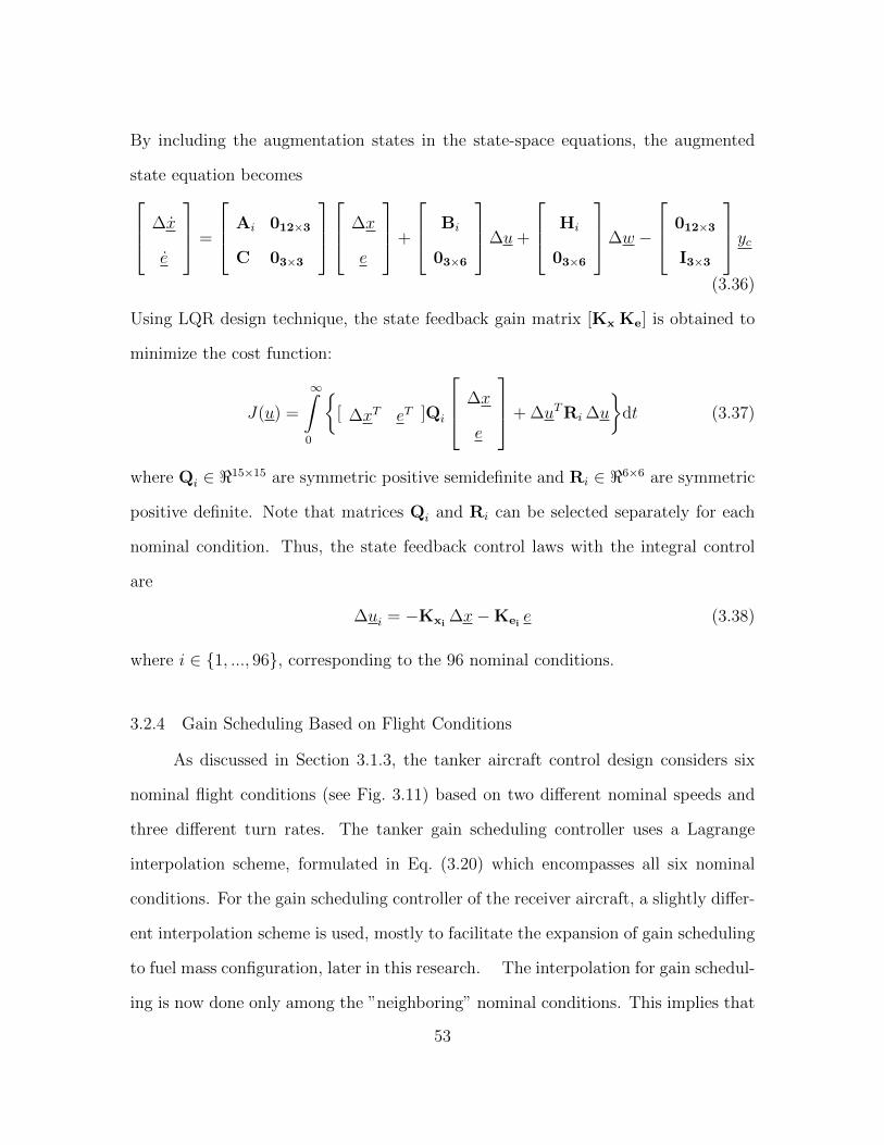
By including the augmentation states in the state-space equations, the augmented
state equation becomes ∆x
e
=
Ai 012×3
C 03×3
∆x
e
+
Bi
03×6
∆u+
Hi
03×6
∆w −
012×3
I3×3
yc(3.36)
Using LQR design technique, the state feedback gain matrix [Kx Ke] is obtained to
minimize the cost function:
J(u) =
∞∫0
{[ ∆xT eT ]Qi
∆x
e
+ ∆uTRi ∆u
}dt (3.37)
where Qi ∈ <15×15 are symmetric positive semidefinite and Ri ∈ <6×6 are symmetric
positive definite. Note that matrices Qi and Ri can be selected separately for each
nominal condition. Thus, the state feedback control laws with the integral control
are
∆ui = −Kxi∆x−Kei e (3.38)
where i ∈ {1, ..., 96}, corresponding to the 96 nominal conditions.
3.2.4 Gain Scheduling Based on Flight Conditions
As discussed in Section 3.1.3, the tanker aircraft control design considers six
nominal flight conditions (see Fig. 3.11) based on two different nominal speeds and
three different turn rates. The tanker gain scheduling controller uses a Lagrange
interpolation scheme, formulated in Eq. (3.20) which encompasses all six nominal
conditions. For the gain scheduling controller of the receiver aircraft, a slightly differ-
ent interpolation scheme is used, mostly to facilitate the expansion of gain scheduling
to fuel mass configuration, later in this research. The interpolation for gain schedul-
ing is now done only among the ”neighboring” nominal conditions. This implies that
53
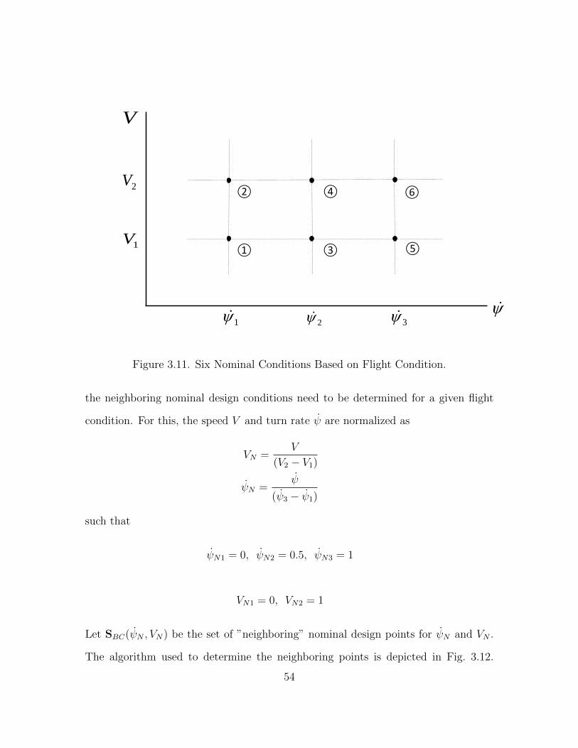
①
②
③
④
⑤
⑥
1 2 3
1V
2V
V
Figure 3.11. Six Nominal Conditions Based on Flight Condition.
the neighboring nominal design conditions need to be determined for a given flight
condition. For this, the speed V and turn rate ψ are normalized as
VN =V
(V2 − V1)
ψN =ψ
(ψ3 − ψ1)
such that
ψN1 = 0, ψN2 = 0.5, ψN3 = 1
VN1 = 0, VN2 = 1
Let SBC(ψN , VN) be the set of ”neighboring” nominal design points for ψN and VN .
The algorithm used to determine the neighboring points is depicted in Fig. 3.12.
54

NV
N
0
0
1
10.4 0.60.5
}1{BCS }3,1{BCS
}2{BCS
}3{BCS
}4{BCS
}5{BCS
}6{BCS}4,2{BCS }6,4{BCS
}5,3{BCS
}2,1{BCS }6,5{BCS}4,3{BCS}4,3,2,1{BCS }6,5,4,3{BCS
①
②
③
④
⑤
⑥
Figure 3.12. Neighboring Nominal Design Conditions.
Given a flight condition with (VC , ψC), ”distance” to each ”neighboring” nominal
design point should be computed. This is done along each scheduling variable sepa-
rately. Let (VBCi , ψBCi) be the speed and the turn rate of the given neighboring point,
BC-i. The sets of the nominal values of the scheduling variables used in defining the
nominal design conditions are
SV = {V1, V2}
Sψ ={ψ1, ψ2, ψ3
}Note VBCi ∈ SV and ψBCi ∈ Sψ. For the nominal point, the subsets of the scheduling
variables are defined as
SiV = SV − {VBCi} (3.39)
Siψ
= Sψ −{ψBCi
}(3.40)
55

Then, the Lagrange interpolation coefficients for each scheduling variable is defined
as
aiV =
n(SiV )∏j=1
VC − VjVBCi − Vj
(3.41)
where Vj ∈ SiV , and n(SiV ) is the cardinal of (number of element in) Set SiV . Similarly
aiψ
=
n(Siψ
)∏j=1
ψC − ψjψBCi − ψj
(3.42)
where ψj ∈ Siψ. The Lagrange coefficient for BC-i is defined to be the product of the
individual coefficients as
ai = aiV aiψ
(3.43)
The last step is to normalize the coefficients over all the neighboring points considered
as
ai =ai∑n(SBC)
j=1 aj
where n(SBC) is the cardinal of the set of the neighboring nominal design points.
Finally, the gain scheduling controller is formulated as the linear combination of the
controllers designed for each neighboring point as
u =
n(SBC)∑i=1
aiui
where ui is the linear controller designed for the nominal flight condition BC-i.
The above discussion is further explained in an example. Consider a flight condition
with (VC , ψC) such that the normalized values are
0 < VNC < 1
0.4 < ψNC < 0.6
which implies, as depicted in Fig. 3.12, that the neighboring points are BC-3 and
BC-4, i.e.,
SBC = {3, 4}56

The Lagrange interpolation coefficient with respect to nominal design conditions BC-3
and BC-4 are to be computed. Starting with BC-3, note from Fig. 3.11 that VBC3 = V1
and ψBC3 = ψ2. By Eqs. (3.39) and (3.40), subsets of scheduling variable values are
S3V = {V2}
S3ψ
={ψ1, ψ3
}Then, Eqs. (3.41) and (3.42) imply
a3V =
VC − V2
V1 − V2
a3ψ
=ψC − ψ1
ψ2 − ψ1
· ψC − ψ3
ψ2 − ψ3
Thus, the Lagrange coefficient of design condition BC-3 is
a3 = a3V a
3ψ
Similarly, the Lagrange coefficient of BC-4 is formulated as follows. Note that VBC4 =
V2 and ψBC4 = ψ2. By Eqs. (3.39) and (3.40), the subsets of scheduling variable values
are
S4V = {V1}
S4ψ
={ψ1, ψ3
}Then, Eqs. (3.41) and (3.42) imply
a4V =
VC − V1
V2 − V1
a4ψ
=ψC − ψ1
ψ2 − ψ1
· ψC − ψ3
ψ2 − ψ3
Thus, the Lagrange coefficient of design condition BC-4 is
a4 = a4V a
4ψ
57

Normalization of a3 and a4, by Eq. (3.44), yields
a3 =a3
a3 + a4
a4 =a4
a3 + a4
Finally, the gain scheduling controller is
u = a3u3 + a4u4
where u3 and u4 are the linear controllers designed specifically for nominal conditions
BC-3 and BC-4, respectively.
3.2.5 Determining Number of Nominal Conditions
3.2.5.1 Eigenvalue Analysis
The process of reducing the number of nominal conditions included in the gain
scheduling controller further from 96 are detailed in this section. The main idea is to
replace a group of nominal conditions with a representative one when the linearized
models around those nominal conditions are ”close” to each other in some sense. Ex-
amples of using eigenvalues locations and Bode plots are presented. The eigenvalues
of state matrix Ai in the linearized equation for each of the 96 nominal conditions in
Eq. (3.29) are plotted on the complex domain. If the eigenvalues of multiple cases are
”close” on the complex domain, then the corresponding linear models are considered
to be dynamically similar, and thus only one of those nominal condition is used in the
gain scheduling. The first sets of cases to analyze are the ones with symmetric fuel
tank loading when the aircraft is in straight-level flight condition. For example, case-
57 and case-53 have only fuel tank 1 and 2 full, respectively when ψT,2 and VT,2. When
the eigenvalues of the corresponding state matrices are compared, it is seen that the
eigenvalues are located at exactly the same positions, as expected. This means that
58

only one of these nominal cases will be sufficient to be included in the gain schedul-
ing. The second sets of cases are the ones with symmetric fuel tank loading when the
aircraft is in turning flight condition. For example, case-89 when ψT,3 and VT,2 with
tank 1 full, and case-21 when ψT,1 and VT,2 with tank 2 full are compared. These
cases are symmetrically similar and eigenvalues are located at exactly the same posi-
tion when eigenvalues of the corresponding state matrices are compared, as expected.
The third case are the ones with ”close” to each other to group them together. For
example, case-82 when ψT,3 and VT,2 with tank 4 full, and case-66 when ψT,3 and VT,1
with tank 4 full are compared. These cases are not symmetrically similar, however
when comparing eigenvalues, they are very close together to group them together as
in Fig. 3.13. The last case shows not all the cases fit in the grouping process. When
comparing case-93 and case-91, those are not symmetrically similar and the pattern
of eigenvalue location is different as in Fig 3.14. Case-93 when ψT,3 and VT,2 with
tank 1,and 2 full and case-91 when ψT,3 and VT,2 with tank 1,and 3 full need to be
treated individually.
3.2.5.2 Bode Plot Analysis
To generate Bode plots, input-output pair should be defined and then corre-
sponding transfer function needs to be derived from Ai and Bi matrices. Bode plots
are helping the eigenvalue discussion by showing cases how they are close together
each other or not. Figure 3.15 shows the third case of eigenvalue example for case-
82 and case-66 comparison and figure 3.16 demonstrates the last case of eigenvalue
example for case-93 and case-91 comparison.
59

Figure 3.13. Eigenvalue comparison for case-82 and case-66.
3.2.5.3 Simplified Receiver Gains
Using eigenvalue and Bode analyses the nominal design conditions for the gain
scheduling are reduced from 96 to 16 mass configuration cases. In the gain schedul-
ing algorithm, 16 nominal cases of fuel tank configurations for each of the 6 flight
conditions will be used.
3.2.5.4 Gain Scheduling Controller
Once the nominal cases to be included in the gain scheduling scheme are deter-
mined, as detailed in the previous section, the LQR controllers for each of the nominal
cases are designed as explained in Section 3.2.3. These linear controllers should be
put together for the final implementation based on the scheduling variables of air-
speed, yaw rate and fuel tank configurations. An interpolation function formulated
60

Figure 3.14. Eigenvalue comparison for case-93 and case-91.
for the tanker controller in Eq. (3.20) because of the discrete nature of the scheduling
variable of fuel configuration. This formulation is part of the plan for completion.
61
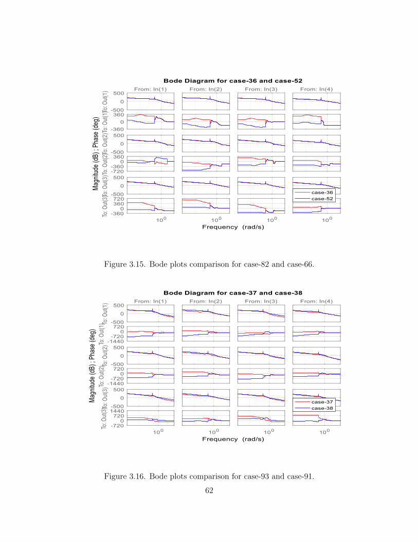
Figure 3.15. Bode plots comparison for case-82 and case-66.
Figure 3.16. Bode plots comparison for case-93 and case-91.
62

Table 3.3. Sixteen Receiver Nominal Conditions
Nominal Condition Flight Condition Tank 1 Tank 2 Tank 3 Tank 4
4 1 0 0 1 111 1 1 0 1 016 1 1 1 1 119 2 0 0 1 024 2 0 1 1 129 2 1 1 0 033 3 0 0 0 036 3 0 0 1 151 4 0 0 1 057 4 1 0 0 060 4 1 0 1 169 5 0 1 0 075 5 1 0 1 083 6 0 0 1 089 6 1 0 0 095 6 1 1 1 0
63
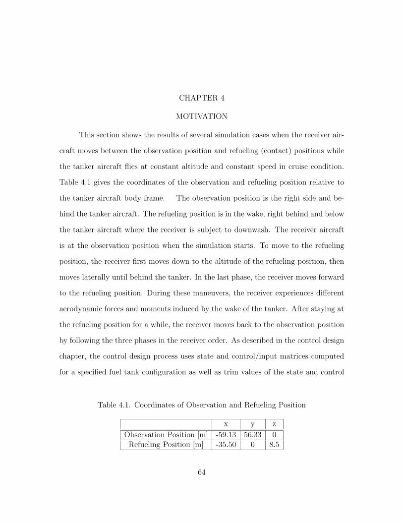
CHAPTER 4
MOTIVATION
This section shows the results of several simulation cases when the receiver air-
craft moves between the observation position and refueling (contact) positions while
the tanker aircraft flies at constant altitude and constant speed in cruise condition.
Table 4.1 gives the coordinates of the observation and refueling position relative to
the tanker aircraft body frame. The observation position is the right side and be-
hind the tanker aircraft. The refueling position is in the wake, right behind and below
the tanker aircraft where the receiver is subject to downwash. The receiver aircraft
is at the observation position when the simulation starts. To move to the refueling
position, the receiver first moves down to the altitude of the refueling position, then
moves laterally until behind the tanker. In the last phase, the receiver moves forward
to the refueling position. During these maneuvers, the receiver experiences different
aerodynamic forces and moments induced by the wake of the tanker. After staying at
the refueling position for a while, the receiver moves back to the observation position
by following the three phases in the receiver order. As described in the control design
chapter, the control design process uses state and control/input matrices computed
for a specified fuel tank configuration as well as trim values of the state and control
Table 4.1. Coordinates of Observation and Refueling Position
x y z
Observation Position [m] -59.13 56.33 0Refueling Position [m] -35.50 0 8.5
64

Table 4.2. Control Allocation (CA)
Cases CA Description
1 No thrust vectoring,only control surfaces used
2 Mix of thrust vectoring andcontrol surfaces used
3 Thrust vectoring and δa used,no δe, and no δr
Table 4.3. Flight Condition and Fuel Mass Configurations - Control Allocation (CA)case is 1.
V [m/s] ψ[deg/s] Tank 1 Tank 2 Tank 3 Tank 4
Control Design 204.39 0 0 0 0 0Simulation 204.39 0 0 0 0 0
variables, again computed for a specific fuel tank configuration. Weighting matrices
Q and R are also tuned based on the matrices of the linear state-space model of the
aircraft. In this chapter, the performance of the closed loop system will be evaluated
in simulation as described above for fuel tank configurations that are different from
the one the control design is based on. This is to evaluate the robustness of the closed-
loop system against the mass and inertia variations. The receiver aircraft simulation
has thrust vectoring capability. In control design, by setting control weighting matrix
R, the levels of thrust vectoring versus of aerodynamic control surfaces, δe and δr, are
specified. Three main control allocation cases are designed and simulated. Table 4.2
gives description of these three cases. The first simulation case is summarized in
Table 4.3. The fuel amounts in the tanks are expressed as percent of the maximum
fuel capacity of the corresponding tank, i.e., 0% implies empty fuel tank and 100%
means full fuel tank. In this simulation, aircraft has the same fuel tank configuration
in simulation as in the control design.
65

Figure 4.1. Commanded and actual trajectory when fuel mass configuration is [0 0 00] in control design and [0 0 0 0] in simulation (CA-1).
Figure 4.2. Control variables when fuel mass configuration is [0 0 0 0] in controldesign and [0 0 0 0] in simulation (CA-1).
Simulation results are shown in Figs. 4.1- 4.5. Fig. 4.1 shows that the controller
successfully moves the receiver aircraft through the commanded trajectory. Fig. 4.2
66

Figure 4.3. Airspeed, sideslip angle and angle of attack when fuel mass configurationis [0 0 0 0] in control design and [0 0 0 0] in simulation (CA-1).
Figure 4.4. Angular velocity and Euler angles when fuel mass configuration is [0 0 00] in control design and [0 0 0 0] in simulation (CA-1).
shows the variation of the control variables through the maneuver. Since the control
allocation case in this simulation is CA-1, no thrust vectoring is used as δy and δz stay
67
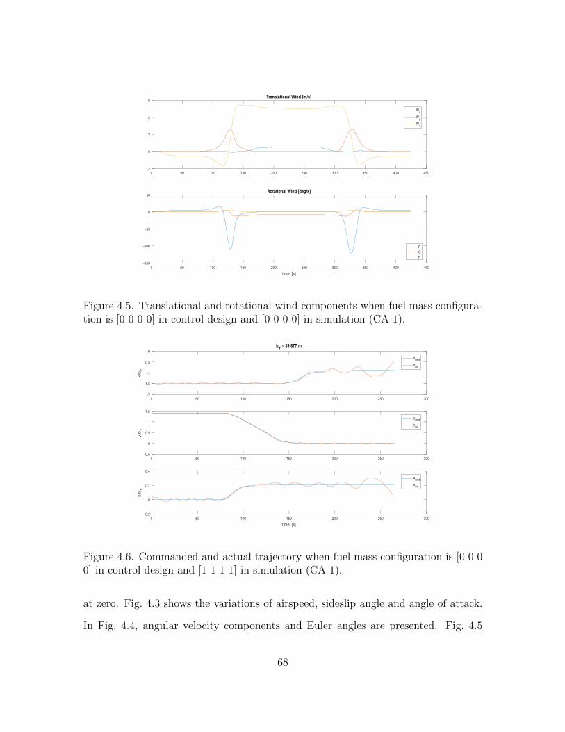
Figure 4.5. Translational and rotational wind components when fuel mass configura-tion is [0 0 0 0] in control design and [0 0 0 0] in simulation (CA-1).
Figure 4.6. Commanded and actual trajectory when fuel mass configuration is [0 0 00] in control design and [1 1 1 1] in simulation (CA-1).
at zero. Fig. 4.3 shows the variations of airspeed, sideslip angle and angle of attack.
In Fig. 4.4, angular velocity components and Euler angles are presented. Fig. 4.5
68
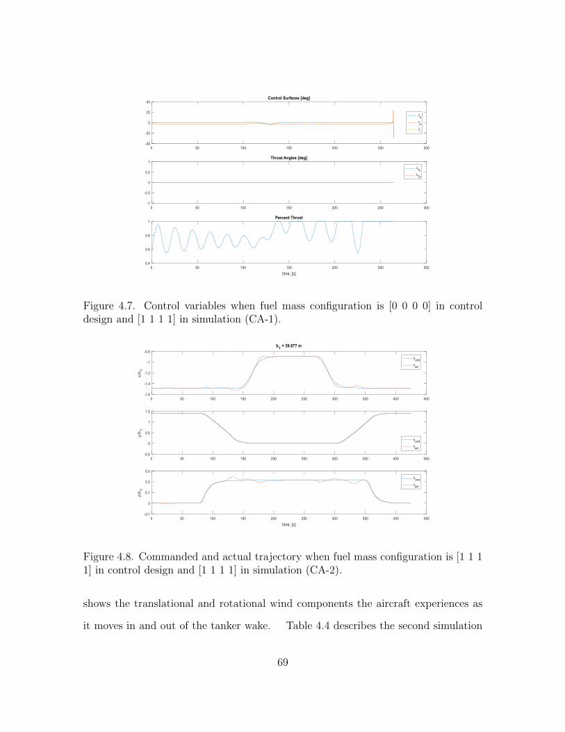
Figure 4.7. Control variables when fuel mass configuration is [0 0 0 0] in controldesign and [1 1 1 1] in simulation (CA-1).
Figure 4.8. Commanded and actual trajectory when fuel mass configuration is [1 1 11] in control design and [1 1 1 1] in simulation (CA-2).
shows the translational and rotational wind components the aircraft experiences as
it moves in and out of the tanker wake. Table 4.4 describes the second simulation
69

Figure 4.9. Control variables when fuel mass configuration is [1 1 1 1] in controldesign and [1 1 1 1] in simulation (CA-2).
Figure 4.10. Commanded and actual trajectory when fuel mass configuration is [1 11 1] in control design and [0 0 0 0] in simulation (CA-2).
case. The control design is the same as the first case above, i.e., all fuel tanks are
considered empty. In the simulated flight, the fuel tanks are all full. That is, the fuel
70

Figure 4.11. Control variables when fuel mass configuration is [1 1 1 1] in controldesign and [0 0 0 0] in simulation (CA-2).
Figure 4.12. Control variables when fuel mass configuration is [1 1 1 1] in controldesign and [0 0.1 0.8 0.1] in simulation (CA-1).
mass configuration in flight is different from the design configuration. Figs. 4.6 and
4.7 show the result of this simulation. Note that the maneuver cannot be completed.
71

Figure 4.13. Angular velocity and Euler angles when fuel mass configuration is [1 11 1] in control design and [0 0.1 0.8 0.1] in simulation (CA-1).
Figure 4.14. Angular velocity and Euler angles when fuel mass configuration is [1 0.10.8 0.1] in control design and [1 0.1 0.8 0.1] in simulation (CA-1).
The controller designed with all empty fuel tank configuration fails to fly the aircraft
with all fuel tanks full. Since the controller in the above case could not fly the aircraft
72
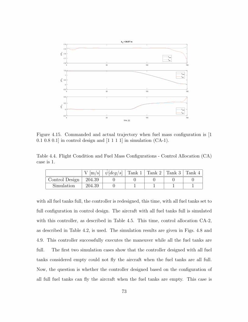
Figure 4.15. Commanded and actual trajectory when fuel mass configuration is [10.1 0.8 0.1] in control design and [1 1 1 1] in simulation (CA-1).
Table 4.4. Flight Condition and Fuel Mass Configurations - Control Allocation (CA)case is 1.
V [m/s] ψ[deg/s] Tank 1 Tank 2 Tank 3 Tank 4
Control Design 204.39 0 0 0 0 0Simulation 204.39 0 1 1 1 1
with all fuel tanks full, the controller is redesigned, this time, with all fuel tanks set to
full configuration in control design. The aircraft with all fuel tanks full is simulated
with this controller, as described in Table 4.5. This time, control allocation CA-2,
as described in Table 4.2, is used. The simulation results are given in Figs. 4.8 and
4.9. This controller successfully executes the maneuver while all the fuel tanks are
full. The first two simulation cases show that the controller designed with all fuel
tanks considered empty could not fly the aircraft when the fuel tanks are all full.
Now, the question is whether the controller designed based on the configuration of
all full fuel tanks can fly the aircraft when the fuel tanks are empty. This case is
73

Table 4.5. Flight Condition and Fuel Mass Configurations - Control Allocation (CA)case is 2.
V [m/s] ψ[deg/s] Tank 1 Tank 2 Tank 3 Tank 4
Control Design 204.39 0 1 1 1 1Simulation 204.39 0 1 1 1 1
Table 4.6. Flight Condition and Fuel Mass Configurations - Control Allocation (CA)case is 2.
V [m/s] ψ[deg/s] Tank 1 Tank 2 Tank 3 Tank 4
Control Design 204.39 0 1 1 1 1Simulation 204.39 0 0 0 0 0
summarized in Table 4.6 and the simulation results are shown in Figs. 4.10 and 4.11.
The results show that controller designed for the heaviest configuration cannot fly the
lightest configuration through the refueling maneuver. Another simulation case,
described in Table 4.7, shows the performance when the aircraft fuel configuration is
asymmetric. The controller designed based on the mass configuration of all fuel tanks
full is enable to complete the maneuver in this asymmetric fuel loading. However,
as shown in Figs. 4.12 and 4.13, the aircraft experiences high frequency, oscillation
in its response, especially in roll motion and aileron deflection. If the controller is
designed based on this specific asymmetric fuel configuration, the response is much
better, without any oscillation, as shown in Fig. 4.14. This controller, however, fails
Table 4.7. Flight Condition and Fuel Mass Configurations - Control Allocation (CA)case is 1.
V [m/s] ψ[deg/s] Tank 1 Tank 2 Tank 3 Tank 4
Control Design 204.39 0 1 1 1 1Simulation 204.39 0 1 0.1 0.8 0.1
74

to complete the maneuver when the aircraft fuel configuration in flight is different
from the design configuration.
75
CHAPTER 5
GAIN SCHEDULING BASED ON FUEL MASS CONFIGURATION
In Section 3.2.4, the gain scheduling was done based on flight condition, which
is defined in terms of speed V and turn rate ψ. The previous section has shown that
the controller that is designed based on a specific mass configuration may not work
when the aircraft flies with a different mass configuration. The mass configuration
is defined in terms of amount of fuel in the fuel tanks; more specifically, in terms
of the percent of fuel amount in each fuel tank relative to the fuel capacity of the
corresponding fuel tank. This section presents the approach taken to expand the
gain scheduling to include the mass configuration of the aircraft. The specific aircraft
considered has four fuel tanks. Percent fuel in each fuel tank is denoted by m1,m2,m3
and m4, which are considered gain scheduling variables in addition to V and ψ, which
are the gain scheduling variables to define the flight condition. Since the four fuel
tank percentages are part of the gain scheduling variables, the nominal value set for
each fuel mass is defined, similar to SV and Sψ in Section 3.2.4 as
Sm1 = {0, 1}
Sm2 = {0, 1} (5.1)
Sm3 = {0, 1}
Sm4 = {0, 1}
76
where note that only empty and full fuel amounts are considered based on the eigen-
value and Bode analyses, presented in Section 3.2.5. A mass configuration is defined
as
Cm = {(m1,m2,m3,m4) : m1 ∈ Sm1 , m2 ∈ Sm2 , m3 ∈ Sm3 , m4 ∈ Sm4}
The nominal design points are redefined for this section to include mass configu-
ration in addition to flight condition (V, ψ) as (V, ψ,Cm). Let (VBCi, ψBCi,CmBCi)
be the flight condition and mass configuration of nominal design point BC-i. Let
(VC , ψC ,CmC ) be the current flight condition and mass configuration. The first step
is to determine the ”neighboring” nominal design conditions SBC based on the current
flight condition (VC , ψC). This is done using the algorithm introduced in Section 3.2.4,
and depicted in Fig. 3.12. This approach requires that there are at least two nominal
points in SBC with the same nominal flight condition, and with distinct mass con-
figurations. The ”mass distance” from the current mass configuration to each of the
nominal point in SBC is computed as
dCmBCi = ‖ CmC −CmBCi ‖
=
√√√√ 4∑j=1
(mjBCi −mjC )2 (5.2)
Based on the ”mass distance”, the subset of SBC with two ”closest” ones to
the current mass configuration for each flight condition is established. This subset is
denoted as SBC . For nominal condition BC − i ∈ SBC , the Lagrange interpolation
coefficients for speed V and turn rate ψC , aiV and aiψ, are computed as before, by
Eqs. (3.41) and (3.42), respectively. The Lagrange interpolation coefficient for mass
configuration can similarly be computed as
aim =4∏j=1
mjC −mj
mjBCi −mj
(5.3)
77
where mj ∈{Smj −mjBCi
}. That is, when mjBCi = 0, mj = 1, and when mjBCi = 1,
mj = 0, since Smj = {1, 0} as defined in Eq. (5.1).
Based on the eigenvalue and Bode analyses, only empty and full fuel tank
configurations are considered for nominal design conditions. Since there are four
fuel tanks, 24 = 16 combinations of fuel tank configurations for each of the 6 flight
conditions. However, as the eigenvalue and Bode analyses further suggested, not
all 16 mass configurations are included in the set of nominal design conditions for
the gain scheduling. In fact, as stated above, the gain scheduling approach taken in
this research requires only at least 2 mass configurations per nominal flight condition.
While this is done to reduce the computational complexity, it brings about a potential
issue with the Lagrange interpolation scheme formulated in Eq. (5.3). If the current
mass configuration happens to be one of the 16 possible mass configurations, then aim
in Eq. (5.3) will be 1 for that mass configuration, and aim will be 0 for all 15 others.
When this specific mass configuration is not one of the nominal design points in SBC ,
i.e., SBC consists of design points with aim = 0, then the scheduling coefficients for
all design points in SBC and thus in SBC will be zero. Thus, the gain scheduling
controller will fail by simply generating zeros for all control variables. For such
cases, an alternative aim calculation is developed. This approach employs the ”mass
distance” as formulated in Eq. (5.2).
aim = 1− dCmBCi∑2j=1 dCmBCj(VBCi, ψBCi)
(5.4)
where dCmBCj(VBCi, ψBCi) indicates the ”mass distances” of the design points with
the same flight conditions as BC-i. The formulation in Eq. (5.4) defines the mass
gain scheduling coefficient in a way similar to the Lagrange interpolation coefficient
in Eq. (5.3) in that as the mass configuration approaches that of BC-i, aim increases
toward 1.
78

Once the speed, turn rate, and mass configuration coefficients are computed
individually, the gain scheduling interpolation coefficients for each nominal design is
computed by their product as
ai = aiV aiψaim
As done in Section 3.2.4, the next step is normalization of these coefficients over all
design points considered as
ai =ai∑n(SBC)
j=1 aj
where n(SBC) is the cardinal of set SBC .
Finally, as done in Section 3.2.4, the gain scheduling controller is formulated as
the linear combination of the controllers designed for each neighboring point as
u =
n(SBC)∑i=1
ai ui
where ui is the linear controller designed for the nominal flight condition BC-i.
79

CHAPTER 6
SIMULATION RESULTS
In the earlier section, it was shown that the controller designed based on a
specific fuel mass configuration may not work for the aircraft flying with different
fuel mass configurations. That is why the gain scheduling controller was expanded
to include various sets of mass configurations. This chapter is to demonstrate the
performance of this controller, first for fuel mass configurations with which the aerial
refueling maneuvers could not be (satisfactorily) completed with one single mass con-
figuration based controller. Further, various other simulation cases will be prosecuted
to demonstrate the performance and robustness of the controller. Table 6.1 lists the
simulation cases presented in this section. The flight condition chosen is flight con-
dition 4, i.e., VT,2 = 204.39m/s and ψT,2 = 0deg/s. Note that in the gain scheduling
controller, for this flight condition, three fuel mass configurations are included. These
are [0 0 1 0], [1 0 0 0], and [1 0 1 1]. The cases simulated here are none of these three
configurations, and thus the gain scheduling performance is demonstrated for mass
configurations not included in the control design. In Table 6.1, the first three cases
are when the aircraft performs the aerial refueling maneuver when the fuel tanks are
empty. Each case uses one of the three control allocation cases. Figs. 6.1- 6.4 show
the simulation results when the control allocation is CA-1. The controller successfully
completes the maneuver even if the fuel mass configuration is not one of the nominal
design cases. Note that, especially, δe is not zero initially before the refueling ma-
neuver starts. This is because the control variables use trim values from the nominal
design cases and all three nominal design cases for this flight condition (zero turn rate
80
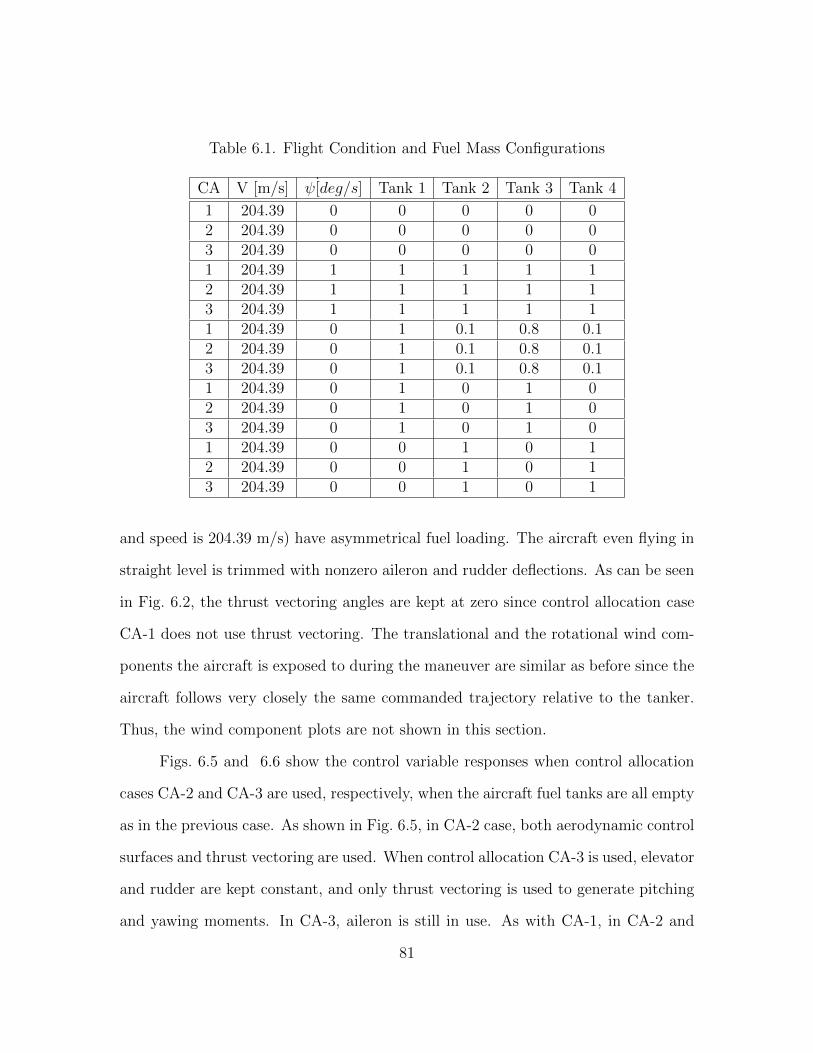
Table 6.1. Flight Condition and Fuel Mass Configurations
CA V [m/s] ψ[deg/s] Tank 1 Tank 2 Tank 3 Tank 4
1 204.39 0 0 0 0 02 204.39 0 0 0 0 03 204.39 0 0 0 0 01 204.39 1 1 1 1 12 204.39 1 1 1 1 13 204.39 1 1 1 1 11 204.39 0 1 0.1 0.8 0.12 204.39 0 1 0.1 0.8 0.13 204.39 0 1 0.1 0.8 0.11 204.39 0 1 0 1 02 204.39 0 1 0 1 03 204.39 0 1 0 1 01 204.39 0 0 1 0 12 204.39 0 0 1 0 13 204.39 0 0 1 0 1
and speed is 204.39 m/s) have asymmetrical fuel loading. The aircraft even flying in
straight level is trimmed with nonzero aileron and rudder deflections. As can be seen
in Fig. 6.2, the thrust vectoring angles are kept at zero since control allocation case
CA-1 does not use thrust vectoring. The translational and the rotational wind com-
ponents the aircraft is exposed to during the maneuver are similar as before since the
aircraft follows very closely the same commanded trajectory relative to the tanker.
Thus, the wind component plots are not shown in this section.
Figs. 6.5 and 6.6 show the control variable responses when control allocation
cases CA-2 and CA-3 are used, respectively, when the aircraft fuel tanks are all empty
as in the previous case. As shown in Fig. 6.5, in CA-2 case, both aerodynamic control
surfaces and thrust vectoring are used. When control allocation CA-3 is used, elevator
and rudder are kept constant, and only thrust vectoring is used to generate pitching
and yawing moments. In CA-3, aileron is still in use. As with CA-1, in CA-2 and
81

Figure 6.1. Commanded and actual trajectory when fuel mass configuration in sim-ulation is [0 0 0 0], (CA-1).
CA-3, the aircraft can successfully completes the refueling maneuver with empty fuel
tank configuration even if this fuel configuration is not one of the nominal design
cases. The gain scheduling controller is also evaluated when the aircraft is at
its heaviest configuration, i.e., all fuel tanks are full. This is done with all control
allocation cases. The results are presented in Figs. 6.7- 6.12. Figs. 6.7- 6.8 show
CA-1; Figs. 6.9- 6.10 show CA-2; Figs. 6.11- 6.12 show CA-3. The other variables are
not shown as their responses are similar to previously discussed corresponding cases.
Note that this mass configuration is also different from any of the mass configuration
included in the control design. In all three control allocation cases, the aircraft
completes the maneuver successfully. The aileron responses are similar in all three
cases. The elevator and rudder use is reduced while thrust vectoring use is increased
82

Figure 6.2. Control variables when fuel mass configuration in simulation is [0 0 0 0],(CA-1).
as the control allocation shifts from CA-1 to CA-2, to CA-3. The thrust responses
in all three cases are very similar. Since the aircraft is heaviest, the thrust gets close
to saturation at times during the maneuver. Yaw angle deviations are the largest
in CA-1 case and the smallest in CA-3 case. The other three
fuel mass configuration cases described in Table 6.1, [1 0.1 0.8 0.1], [1 0 1 0], and
[0 1 0 1] are all asymmetric cases. The controller with all three control allocation
cases can successfully complete the refueling maneuver despite the asymmetric mass
distribution. The case [1 0.1 0.8 0.1] is one of the cases that was shown to fail before,
when the control design was based on one fuel mass configuration. The other two, [1
0 1 0] and [0 1 0 1], has even greater asymmetry. Still the controller with only three
nominal design cases included can control the aircraft in different mass distributions.
83

Figure 6.3. Airspeed, sideslip angle and angle of attack when fuel mass configurationin simulation is [0 0 0 0], (CA-1).
Figs. 6.13- 6.14, 6.15- 6.16, and 6.17- 6.18 present the responses of control variables,
airspeed, sideslip angle, and angle of attack in CA-1 cases with mass configurations
[1 0.1 0.8 0.1], [1 0 1 0], and [0 1 0 1], respectively.
84

Figure 6.4. Angular velocity and Euler angles when fuel mass configuration in simu-lation is [0 0 0 0], (CA-1).
85

Figure 6.5. Control variables when fuel mass configuration in simulation is [0 0 0 0],(CA-2).
Figure 6.6. Control variables when fuel mass configuration in simulation is [0 0 0 0],(CA-3).
86
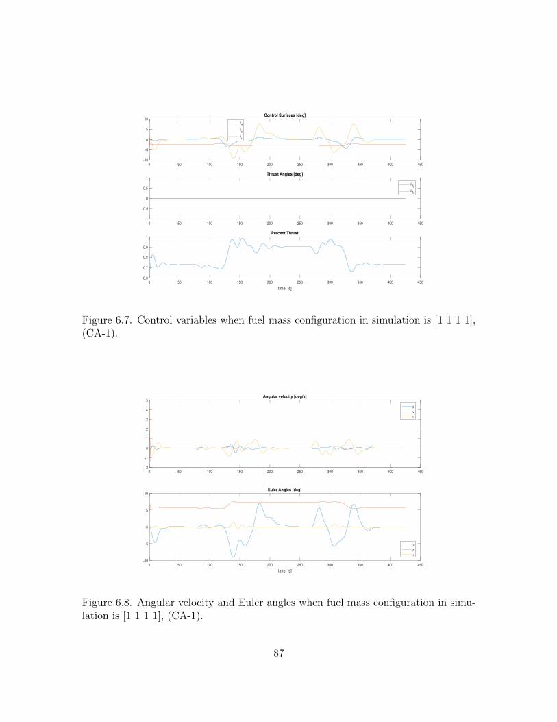
Figure 6.7. Control variables when fuel mass configuration in simulation is [1 1 1 1],(CA-1).
Figure 6.8. Angular velocity and Euler angles when fuel mass configuration in simu-lation is [1 1 1 1], (CA-1).
87

Figure 6.9. Control variables when fuel mass configuration in simulation is [1 1 1 1],(CA-2).
Figure 6.10. Angular velocity and Euler angles when fuel mass configuration in sim-ulation is [1 1 1 1], (CA-2).
88

Figure 6.11. Control variables when fuel mass configuration in simulation is [1 1 1 1],(CA-3).
Figure 6.12. Angular velocity and Euler angles when fuel mass configuration in sim-ulation is [1 1 1 1], (CA-3).
89

Figure 6.13. Control variables when fuel mass configuration in simulation is [1 0.10.8 0.1], (CA-1).
Figure 6.14. Airspeed, sideslip angle and angle of attack when fuel mass configurationin simulation is [1 0.1 0.8 0.1], (CA-1).
90

Figure 6.15. Control variables when fuel mass configuration in simulation is [1 0 1 0],(CA-1).
Figure 6.16. Airspeed, sideslip angle and angle of attack when fuel mass configurationin simulation is [1 0 1 0], (CA-1).
91

Figure 6.17. Control variables when fuel mass configuration in simulation is [0 1 0 1],(CA-1).
Figure 6.18. Airspeed, sideslip angle and angle of attack when fuel mass configurationin simulation is [0 1 0 1], (CA-1).
92

CHAPTER 7
CONCLUSION AND FUTURE WORK
This research effort focuses on addressing the issue of mass/inertia variation
in aerial refueling and formation flight by expanding the gain scheduling scheme to
include fuel mass in each fuel tank among the scheduling variables in addition to
airspeed and turn rate. The fuel mass in each fuel tank is considered as state variable
in addition to the standard states associated with aircraft dynamics. All possible
fuel distributions, both symmetric and asymmetric, are considered in trim analyses
of the aircraft in straight level and steady-turn flight conditions at constant altitude
and constant airspeed. The gain scheduling controller design requires the definition
of trim conditions in terms of the fuel amounts in fuel tanks for each set of turn rate
and speed. The three turn rates (zero, right turn, and left turn) and two speed values
result in six nominal flight conditions, as done with the tanker aircraft.
For the receiver aircraft, the number of mass/inertia configurations to be in-
cluded in the set of trim conditions should be determined. The objective is to keep the
number of such fuel tank configurations small while making sure that they will cover
the whole span of the mass/inertia variation of the receiver aircraft. To reduce the
number of cases included in the gain scheduling, similar cases are combined. In each
possible case, the equations of motion are linearized to obtain the state and control
matrices. From the state and control matrices, various transfer functions are com-
puted. Similarity of the cases are determined based on the eigenvalue locations of the
state matrix and Bode plots of the transfer functions. The specific aircraft considered
is a tailless delta wing aircraft with thrust vectoring capability. The eigenvalue and
93

Bode analyses show that variations in the dynamics of the aircraft are not significant
for fractional changes in the fuel amounts in each tank. This imply that only com-
pletely empty and completely full fuel tanks are sufficient to capture the variation in
the dynamics. This specific aircraft has four fuel tanks, which imply that there are
still 24 = 16 fuel mass configurations per flight condition. Eigenvalue and Bode plot
analyses further demonstrate that not all 16 mass configurations are needed. Two or
three mass configurations for each flight conditions are eventually kept for the gain
scheduling control design.
An LQR-based MIMO (Multi Input Multi Output) integral control is designed
for each nominal flight and mass configuration. An interpolation scheme based on
the ”mass distance” is developed to combine this linear controllers into the gain
scheduling controller. The ”mass distance” is defined as the norm of the differences
between the current fuel tank amounts and those of each nominal mass configuration.
The Lagrange interpolation scheme, as commonly used in gain scheduling, assumes
that all possible combinations of fuel mass configurations are included among the
nominal conditions used in gain scheduling. However, as stated above, only a subset
of possible mass configurations is included in gain scheduling. While this is done
to reduce the computational complexity, it brings about a potential issue with the
Lagrange interpolation. If the current mass configuration of the aircraft is one of the
16 fuel mass configurations stated above, but not included in the subset determined
after eliminating ”similar” cases, the Lagrange interpolation scheme computes all
the coefficients of the cases included as zero. This would cause the gain scheduling
controller to fail by simply generating zeros for all control variables. To avoid this
issue, an alternative interpolation method is developed for mass configurations by
employing the ”mass distance” discussed above.
94

The receiver controller was tuned in three control allocation cases: (1) no thrust
vectoring; only aerodynamic control effects in use, (2) both aerodynamic effectors and
thrust vectoring in use, and (3) no elevator or rudder used; only thrust vectoring and
aileron in use. The performance of the gain scheduling controller is evaluated through
the aerial refueling maneuver when the receiver moves between the observation po-
sition, point on the side and behind the tanker, and the refueling position, a point
right behind and slightly below the tanker. The simulation results first of all demon-
strates that a linear controller designed based on a nominal flight condition and mass
configuration cannot safely complete the refueling maneuver when the aircraft has
a different mass configuration. The simulation results further shows that the gain
scheduling controller employing mass configuration as additional scheduling variables
can successfully carry out the refueling maneuver with various symmetric and asym-
metric fuel tank configuration. All three control allocation schemes employing the
mass-configuration-based gain scheduling perform similarly in terms of tracking the
commanded trajectory while the control responses vary accordingly.
There are various directions for future research effort in this area. The location
of Eigenvalues and Bode plots are used to determine whether two linear modes are
close to each other. A more formal way of quantifying how close linear models should
be developed in deciding whether to include in the gain scheduling scheme. The
receiver aircraft considered is a tailless delta wing aircraft, which is a small aircraft
geometrically and thus the fuel tanks are close to the origin of the body frame. It is
expected that the effect of the fuel mass variation will be more profound when larger
receiver aircraft is considered. The analyses and the design effort can be repeated
for a larger aircraft, for example, another KC-135 flying behind the tanker KC-135
aircraft. In this research numerous simulations are carried out in evaluating the
performance of the gain scheduling controller. However, in each simulation run, the
95

mass configuration is fixed. The performance of the gain scheduling can be evaluated
when the mass configuration is varying during simulation.
96

APPENDIX A
NOMINAL CONDITIONS OF THE RECEIVER AIRCRAFT
97

Table A.1. Nominal Conditions (1-32) of the Receiver by Turn rate, Airspeed, andReceiver Fuel Tanks Status
Nominal Flight Tank 1 Tank 2 Tank 3 Tank 4Conditon Case
1 1 0 0 0 02 1 0 0 0 13 1 0 0 1 04 1 0 0 1 15 1 0 1 0 06 1 0 1 0 17 1 0 1 1 08 1 0 1 1 19 1 1 0 0 010 1 1 0 0 111 1 1 0 1 012 1 1 0 1 113 1 1 1 0 014 1 1 1 0 115 1 1 1 1 016 1 1 1 1 1
17 2 0 0 0 018 2 0 0 0 119 2 0 0 1 020 2 0 0 1 121 2 0 1 0 022 2 0 1 0 123 2 0 1 1 024 2 0 1 1 125 2 1 0 0 026 2 1 0 0 127 2 1 0 1 028 2 1 0 1 129 2 1 1 0 030 2 1 1 0 131 2 1 1 1 032 2 1 1 1 1
98

Table A.2. Nominal Conditions (33-64) of the Receiver by Turn rate, Airspeed, andReceiver Fuel Tanks Status
Nominal Flight Tank 1 Tank 2 Tank 3 Tank 4Conditon Case
33 3 0 0 0 034 3 0 0 0 135 3 0 0 1 036 3 0 0 1 137 3 0 1 0 038 3 0 1 0 139 3 0 1 1 040 3 0 1 1 141 3 1 0 0 042 3 1 0 0 143 3 1 0 1 044 3 1 0 1 145 3 1 1 0 046 3 1 1 0 147 3 1 1 1 048 3 1 1 1 1
49 4 0 0 0 050 4 0 0 0 151 4 0 0 1 052 4 0 0 1 153 4 0 1 0 054 4 0 1 0 155 4 0 1 1 056 4 0 1 1 157 4 1 0 0 058 4 1 0 0 159 4 1 0 1 060 4 1 0 1 161 4 1 1 0 062 4 1 1 0 163 4 1 1 1 064 4 1 1 1 1
99

Table A.3. Nominal Conditions (65-96) of the Receiver by Turn rate, Airspeed, andReceiver Fuel Tanks Status
Nominal Flight Tank 1 Tank 2 Tank 3 Tank 4Conditon Case
65 5 0 0 0 066 5 0 0 0 167 5 0 0 1 068 5 0 0 1 169 5 0 1 0 070 5 0 1 0 171 5 0 1 1 072 5 0 1 1 173 5 1 0 0 074 5 1 0 0 175 5 1 0 1 076 5 1 0 1 177 5 1 1 0 078 5 1 1 0 179 5 1 1 1 080 5 1 1 1 1
81 6 0 0 0 082 6 0 0 0 183 6 0 0 1 084 6 0 0 1 185 6 0 1 0 086 6 0 1 0 187 6 0 1 1 088 6 0 1 1 189 6 1 0 0 090 6 1 0 0 191 6 1 0 1 092 6 1 0 1 193 6 1 1 0 094 6 1 1 0 195 6 1 1 1 096 6 1 1 1 1
100

APPENDIX B
EIGENVALUES OF THE RECEIVER AIRCRAFT
101
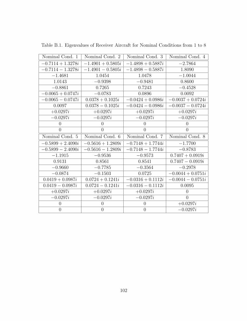
Table B.1. Eigenvalues of Receiver Aircraft for Nominal Conditions from 1 to 8
Nominal Cond. 1 Nominal Cond. 2 Nominal Cond. 3 Nominal Cond. 4
−0.7114 + 1.3278i −1.4901 + 0.5805i −1.4898 + 0.5887i −2.7864−0.7114− 1.3278i −1.4901− 0.5805i −1.4898− 0.5887i 1.8090
−1.4681 1.0454 1.0478 −1.00441.0143 −0.9398 −0.9481 0.8600−0.8861 0.7265 0.7243 −0.4528
−0.0065 + 0.0747i −0.0783 0.0896 0.0092−0.0065− 0.0747i 0.0378 + 0.1025i −0.0424 + 0.0986i −0.0037 + 0.0724i
0.0097 0.0378− 0.1025i −0.0424− 0.0986i −0.0037− 0.0724i+0.0297i +0.0297i +0.0297i +0.0297i−0.0297i −0.0297i −0.0297i −0.0297i
0 0 0 00 0 0 0
Nominal Cond. 5 Nominal Cond. 6 Nominal Cond. 7 Nominal Cond. 8
−0.5899 + 2.4090i −0.5616 + 1.2809i −0.7148 + 1.7744i −1.7700−0.5899− 2.4090i −0.5616− 1.2809i −0.7148− 1.7744i −0.8783
−1.1915 −0.9536 −0.9573 0.7407 + 0.0919i0.9131 0.8561 0.8541 0.7407− 0.0919i−0.9660 −0.7785 −0.3564 −0.2978−0.0874 −0.1503 0.0725 −0.0044 + 0.0751i
0.0419 + 0.0987i 0.0724 + 0.1241i −0.0316 + 0.1112i −0.0044− 0.0751i0.0419− 0.0987i 0.0724− 0.1241i −0.0316− 0.1112i 0.0095
+0.0297i +0.0297i +0.0297i 0−0.0297i −0.0297i −0.0297i 0
0 0 0 +0.0297i0 0 0 −0.0297i
102

Table B.2. Eigenvalues of Receiver Aircraft for Nominal Conditions from 9 to 16
Nominal Cond. 9 Nominal Cond. 10 Nominal Cond. 11 Nominal Cond. 12
−0.5916 + 2.4086i −0.7142 + 1.7743i −0.5690 + 1.2788i −1.7691−0.5916− 2.4086i −0.7142− 1.7743i −0.5690− 1.2788i −0.8794
−1.1926 −0.9591 −0.9437 0.7393 + 0.0882i−0.9641 0.8527 0.8563 0.7393− 0.0882i0.9117 −0.3370 −0.7903 −0.29770.0840 −0.0924 0.1232 −0.0006 + 0.0588i
−0.0419 + 0.1080i 0.0421 + 0.0901i −0.0560 + 0.1516i −0.0006− 0.0588i−0.0419− 0.1080i 0.0421− 0.0901i −0.0560− 0.1516i 0.0045
+0.0297i +0.0297i +0.0297i +0.0297i−0.0297i −0.0297i −0.0297i −0.0297i
0 0 0 00 0 0 0
Nominal Cond. 13 Nominal Cond. 14 Nominal Cond. 15 Nominal Cond. 16
−0.6548 + 3.1745i −0.6096 + 2.4435i −0.6098 + 2.4435i −0.4470 + 1.3133i−0.6548− 3.1745i −0.6096− 2.4435i −0.6098− 2.4435i −0.4470− 1.3133i
−0.8508 −0.8527 −0.8475 −0.78070.8332 0.7769 0.7776 0.7097−0.7806 −0.4269 −0.4556 −0.3947
−0.0065 + 0.0730i −0.1275 1.1031 0.0124−0.0065− 0.0730i 0.0588 + 0.1091i −0.0448 + 0.1308i −0.0033 + 0.0760i
0.0120 0.0588− 0.1091i −0.0448− 0.1308i −0.0033− 0.0760i+0.0297i +0.0297i +0.0297i +0.0297i−0.0297i −0.0297i −0.0297i −0.0297i
0 0 0 00 0 0 0
103
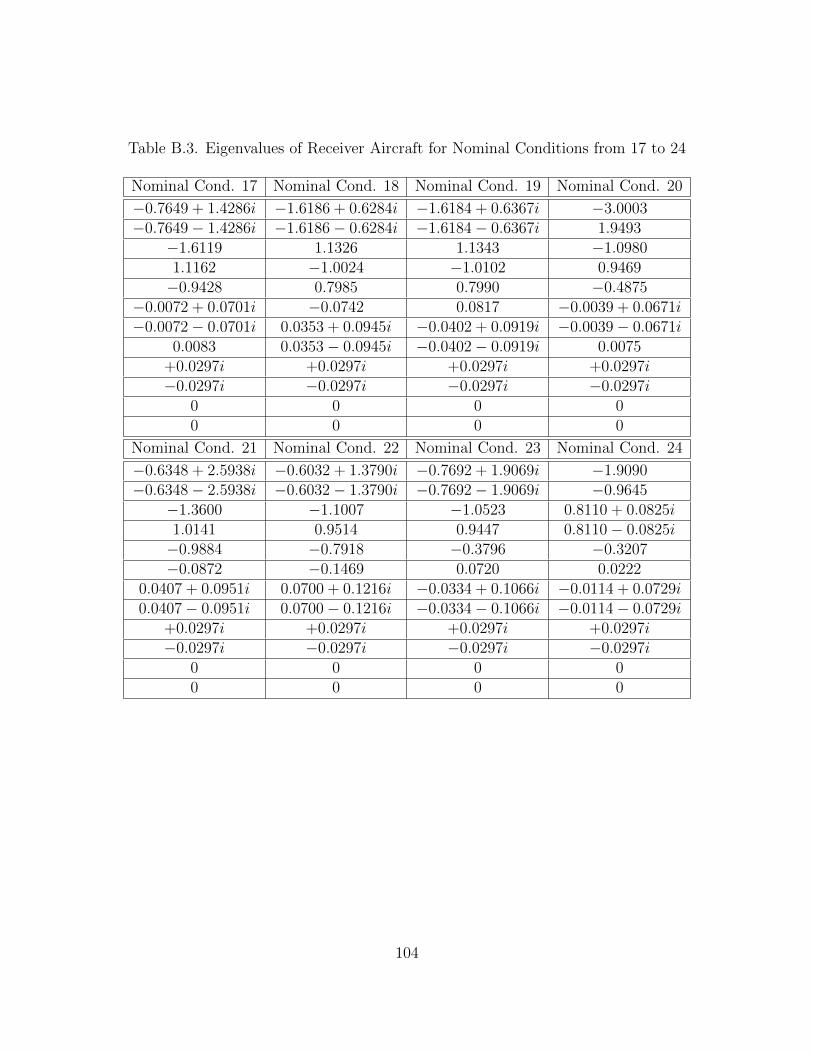
Table B.3. Eigenvalues of Receiver Aircraft for Nominal Conditions from 17 to 24
Nominal Cond. 17 Nominal Cond. 18 Nominal Cond. 19 Nominal Cond. 20
−0.7649 + 1.4286i −1.6186 + 0.6284i −1.6184 + 0.6367i −3.0003−0.7649− 1.4286i −1.6186− 0.6284i −1.6184− 0.6367i 1.9493
−1.6119 1.1326 1.1343 −1.09801.1162 −1.0024 −1.0102 0.9469−0.9428 0.7985 0.7990 −0.4875
−0.0072 + 0.0701i −0.0742 0.0817 −0.0039 + 0.0671i−0.0072− 0.0701i 0.0353 + 0.0945i −0.0402 + 0.0919i −0.0039− 0.0671i
0.0083 0.0353− 0.0945i −0.0402− 0.0919i 0.0075+0.0297i +0.0297i +0.0297i +0.0297i−0.0297i −0.0297i −0.0297i −0.0297i
0 0 0 00 0 0 0
Nominal Cond. 21 Nominal Cond. 22 Nominal Cond. 23 Nominal Cond. 24
−0.6348 + 2.5938i −0.6032 + 1.3790i −0.7692 + 1.9069i −1.9090−0.6348− 2.5938i −0.6032− 1.3790i −0.7692− 1.9069i −0.9645
−1.3600 −1.1007 −1.0523 0.8110 + 0.0825i1.0141 0.9514 0.9447 0.8110− 0.0825i−0.9884 −0.7918 −0.3796 −0.3207−0.0872 −0.1469 0.0720 0.0222
0.0407 + 0.0951i 0.0700 + 0.1216i −0.0334 + 0.1066i −0.0114 + 0.0729i0.0407− 0.0951i 0.0700− 0.1216i −0.0334− 0.1066i −0.0114− 0.0729i
+0.0297i +0.0297i +0.0297i +0.0297i−0.0297i −0.0297i −0.0297i −0.0297i
0 0 0 00 0 0 0
104

Table B.4. Eigenvalues of Receiver Aircraft for Nominal Conditions from 25 to 32
Nominal Cond. 25 Nominal Cond. 26 Nominal Cond. 27 Nominal Cond. 28
−0.6365 + 2.5934i −0.7684 + 1.9067i −0.6114 + 1.3771i −1.9079−0.6365− 2.5934i −0.7684− 1.9067i −0.6114− 1.3771i −0.9653
−1.3600 −1.0536 −1.0967 −0.32061.0130 0.9436 0.9513 0.8105 + 0.0798i−0.9870 −0.3648 −0.7933 0.8105− 0.0798i0.0820 −0.0909 0.1216 −0.0218
−0.0423 + 0.0134i 0.0411 + 0.0879i −0.0572 + 0.1460i 0.0110 + 0.0569i−0.0423− 0.0134i 0.0411− 0.0879i −0.0572− 0.1460i 0.0110− 0.0569i
+0.0297i +0.0297i +0.0297i +0.0297i−0.0297i −0.0297i −0.0297i −0.0297i
0 0 0 00 0 0 0
Nominal Cond. 29 Nominal Cond. 30 Nominal Cond. 31 Nominal Cond. 32
−0.7041 + 3.4165i −0.6554 + 2.6296i −0.6559 + 2.6296i −0.4805 + 1.4135i−0.7041− 3.4165i −0.6554− 2.6296i −0.6559− 2.6296i −0.4805− 1.4135i
−1.0258 −0.9537 −0.9504 −0.87260.9339 0.8692 0.8699 0.7955−0.7618 −0.4552 −0.4759 −0.4182
−0.0066 + 0.0679i −0.1203 −0.0984 0.0098−0.0066− 0.0679i 0.0555 + 0.1045i −0.0450 + 0.1235i −0.0036 + 0.0708i
0.0098 0.0555− 0.1045i −0.0450− 0.1235i −0.0036− 0.0708i+0.0297i +0.0297i +0.0297i +0.0297i−0.0297i −0.0297i −0.0297i −0.0297i
0 0 0 00 0 0 0
105

Table B.5. Eigenvalues of Receiver Aircraft for Nominal Conditions from 33 to 40
Nominal Cond. 33 Nominal Cond. 34 Nominal Cond. 35 Nominal Cond. 36
0 0 0 00 0 0 00 0 0 0
−1.5279 −1.5218 + 0.5860i −1.5218 + 0.5860i 0.86711.0293 −1.5218− 0.5860i −1.5218− 0.5860i −1.0505−0.8405 1.0551 1.0551 −0.41530.0129 −0.8902 −0.8902 −2.7894
0 −0.7298 0.7298 0−0.7115 + 1.3280i 0.0146 0.0146 0.0162−0.7115− 1.3280i 0 0 1.8128−0.0078 + 0.0732i −0.0074 + 0.0714i −0.0074 + 0.0714i −0.0058 + 0.0719i−0.0078− 0.0732i −0.0074− 0.0714i −0.0074− 0.0714i −0.0058− 0.0719i
Nominal Cond. 37 Nominal Cond. 38 Nominal Cond. 39 Nominal Cond. 40
0 0 0 00 0 0 00 0 0 0
−0.5916 + 2.4109i −0.5655 + 1.2815i −0.7134 + 1.7718i −1.7767−0.5916− 2.4109i −0.5655− 1.2815i −0.7134− 1.7718i −0.9169
−1.3206 −1.0842 −0.9992 0.7489 + 0.0915i0.9320 0.8732 0.8677 0.7489− 0.0915i−0.8520 −0.6652 −0.3254 −0.27240.0150 0.0166 +0.0167 0.0185
0 0 0 0−0.0081 + 0.0726i −0.0060 + 0.0738i −0.0054 + 0.0736i −0.0060 + 0.0686i−0.0081− 0.0726i −0.0060− 0.0738i −0.0054− 0.0736i −0.0060− 0.0686i
106

Table B.6. Eigenvalues of Receiver Aircraft for Nominal Conditions from 41 to 48
Nominal Cond. 41 Nominal Cond. 42 Nominal Cond. 43 Nominal Cond. 44
0 0 0 00 0 0 00 0 0 0
−0.5916 + 2.4109i −1.7134 + 1.7718i −0.5655 + 1.2815i −1.7767−0.5916− 2.4109i −1.7134− 1.7718i −0.5655− 1.2815i −0.9169
−1.3206 −0.9992 −1.0842 0.7489 + 0.0915i0.9320 0.8677 0.8732 0.7489− 0.0915i−0.8527 −0.3254 −0.6652 −0.27240.0150 0.0167 0.0166 0.0185
0 0 0 0−0.0081 + 0.0726i −0.0054 + 0.0736i −0.0060 + 0.0738i −0.0060 + 0.0686i−0.0081− 0.0726i −0.0054− 0.0736i −0.0060− 0.0738i −0.0060− 0.0686i
Nominal Cond. 45 Nominal Cond. 46 Nominal Cond. 47 Nominal Cond. 48
0 0 0 00 0 0 00 0 0 0
0.8571 −0.6092 + 2.4444i −0.6092 + 2.4444i 0.7242−1.0201 −0.6092− 2.4444i −0.6092− 2.4444i −0.8506−0.6343 −0.9195 −0.9195 −0.34120.0174 0.7966 0.7966 0.0217
0 −0.3940 −0.3940 0−0.6546 + 3.1759i 0.0192 0.0192 −0.4470 + 1.3138i−0.6546− 3.1759i 0 0 −0.4470− 1.3138i−0.0082 + 0.0725i −0.0063 + 0.0730i −0.0063 + 0.0730i −0.0056 + 0.0743i−0.0082− 0.0725i −0.0063− 0.0730i −0.0063− 0.0730i −0.0056− 0.0743i
107

Table B.7. Eigenvalues of Receiver Aircraft for Nominal Conditions from 49 to 56
Nominal Cond. 49 Nominal Cond. 50 Nominal Cond. 51 Nominal Cond. 52
0 0 0 00 0 0 00 0 0 0
−1.6717 −1.6509 + 0.6342i −1.6509 + 0.6342i 0.95501.1321 −1.6509− 0.6342i −1.6509− 0.6342i −1.1456−0.8979 1.1427 1.1427 −0.44910.0110 −0.9522 −0.9522 −3.0031
0 0.8030 0.8030 0−0.7651 + 1.4287i −0.0074 + 0.0657i −0.0074 + 0.0657i 0.0136−0.7651− 1.4287i −0.0074− 0.0657i −0.0074− 0.0657i 1.9528−0.0083 + 0.0689i 0.0123 0.0123 −0.0059 + 0.0667i−0.0083− 0.0689i 0 0 −0.0059− 0.0667i
Nominal Cond. 53 Nominal Cond. 54 Nominal Cond. 55 Nominal Cond. 56
0 0 0 00 0 0 00 0 0 0
−0.6366 + 2.5957i −0.6075 + 1.3797i −0.7676 + 1.9039i −1.9158−0.6366− 2.5957i −0.6075− 1.3797i −0.7676− 1.9039i −1.0038
−1.4682 −1.2094 −1.0951 0.8199 + 0.0817i1.0340 0.9694 0.9594 0.8199− 0.0817i−0.8964 −0.6990 −0.3501 −0.29450.0126 0.0138 0.0139 0.0152
0 0 0 0−0.0083 + 0.0677i −0.0062 + 0.0691i −0.0057 + 0.0689i −0.0058 + 0.0630i−0.0083− 0.0677i −0.0062− 0.0691i −0.0057− 0.0689i −0.0058− 0.0630i
108
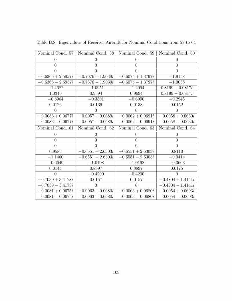
Table B.8. Eigenvalues of Receiver Aircraft for Nominal Conditions from 57 to 64
Nominal Cond. 57 Nominal Cond. 58 Nominal Cond. 59 Nominal Cond. 60
0 0 0 00 0 0 00 0 0 0
−0.6366 + 2.5957i −0.7676 + 1.9039i −0.6075 + 1.3797i −1.9158−0.6366− 2.5957i −0.7676− 1.9039i −0.6075− 1.3797i −1.0038
−1.4682 −1.0951 −1.2094 0.8199 + 0.0817i1.0340 0.9594 0.9694 0.8199− 0.0817i−0.8964 −0.3501 −0.6990 −0.29450.0126 0.0139 0.0138 0.0152
0 0 0 0−0.0083 + 0.0677i −0.0057 + 0.0689i −0.0062 + 0.0691i −0.0058 + 0.0630i−0.0083− 0.0677i −0.0057− 0.0689i −0.0062− 0.0691i −0.0058− 0.0630i
Nominal Cond. 61 Nominal Cond. 62 Nominal Cond. 63 Nominal Cond. 64
0 0 0 00 0 0 00 0 0 0
0.9583 −0.6551 + 2.6303i −0.6551 + 2.6303i 0.8110−1.1460 −0.6551− 2.6303i −0.6551− 2.6303i −0.9414−0.6649 −1.0198 −1.0198 −0.36630.0144 0.8897 0.8897 0.0175
0 −0.4200 −0.4200 0−0.7039 + 3.4178i 0.0157 0.0157 −0.4804 + 1.4141i−0.7039− 3.4178i 0 0 −0.4804− 1.4141i−0.0081 + 0.0675i −0.0063 + 0.0680i −0.0063 + 0.0680i −0.0054 + 0.0693i−0.0081− 0.0675i −0.0063− 0.0680i −0.0063− 0.0680i −0.0054− 0.0693i
109

Table B.9. Eigenvalues of Receiver Aircraft for Nominal Conditions from 65 to 72
Nominal Cond. 65 Nominal Cond. 66 Nominal Cond. 67 Nominal Cond. 68
−0.7114 + 1.3278i −1.4898 + 0.5887i −1.4901 + 0.5805i −2.7864−0.7114− 1.3278i −1.4898− 0.5887i −1.4901− 0.5805i 1.8090
−1.4681 1.0478 1.0454 −1.00431.0143 −0.9481 −0.9398 0.8600−0.8861 0.7243 0.7265 −0.4528
−0.0065 + 0.0747i 0.0896 −0.0783 0.0092−0.0065− 0.0747i −0.0424 + 0.0986i 0.0378 + 0.1025i −0.0037 + 0.0724i
0.0097 −0.0424− 0.0986i 0.0378− 0.1025i −0.0037− 0.0724i+0.0297i +0.0297i +0.0297i +0.0297i−0.0297i −0.0297i −0.0297i −0.0297i
0 0 0 00 0 0 0
Nominal Cond. 69 Nominal Cond. 70 Nominal Cond. 71 Nominal Cond. 72
−0.5916 + 2.4086i −0.5690 + 1.2788i −0.7142 + 1.7743i −1.7691−0.5916− 2.4086i −0.5690− 1.2788i −0.7142− 1.7743i −0.8794
−1.1926 −0.9437 −0.9591 0.7394 + 0.0882i−0.9641 0.8563 0.8521 0.7394− 0.0882i0.9117 −0.7903 −0.3370 −0.29770.0840 0.1232 −0.0924 −0.0006 + 0.0588i
−0.0419 + 0.1080i −0.0560 + 0.1516i 0.0421 + 0.0901i −0.0006− 0.0588i−0.0419− 0.1080i −0.0560− 0.1516i 0.0421− 0.0901i 0.0045
+0.0297i +0.0297i +0.0297i +0.0297i−0.0297i −0.0297i −0.0297i −0.0297i
0 0 0 00 0 0 0
110
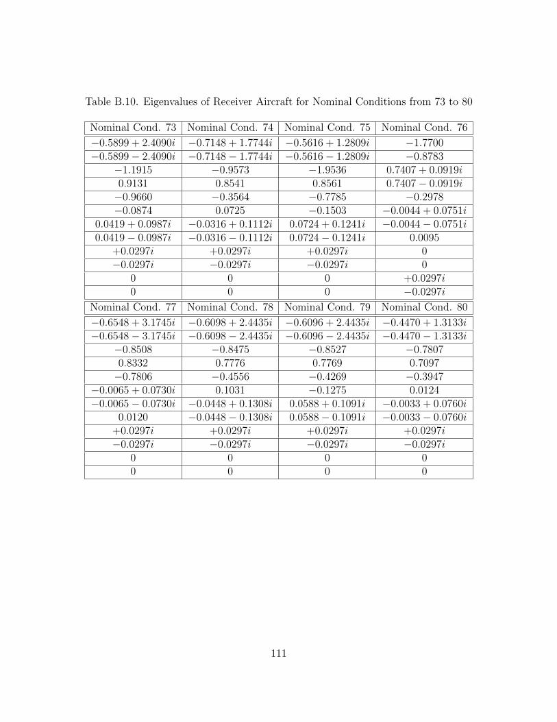
Table B.10. Eigenvalues of Receiver Aircraft for Nominal Conditions from 73 to 80
Nominal Cond. 73 Nominal Cond. 74 Nominal Cond. 75 Nominal Cond. 76
−0.5899 + 2.4090i −0.7148 + 1.7744i −0.5616 + 1.2809i −1.7700−0.5899− 2.4090i −0.7148− 1.7744i −0.5616− 1.2809i −0.8783
−1.1915 −0.9573 −1.9536 0.7407 + 0.0919i0.9131 0.8541 0.8561 0.7407− 0.0919i−0.9660 −0.3564 −0.7785 −0.2978−0.0874 0.0725 −0.1503 −0.0044 + 0.0751i
0.0419 + 0.0987i −0.0316 + 0.1112i 0.0724 + 0.1241i −0.0044− 0.0751i0.0419− 0.0987i −0.0316− 0.1112i 0.0724− 0.1241i 0.0095
+0.0297i +0.0297i +0.0297i 0−0.0297i −0.0297i −0.0297i 0
0 0 0 +0.0297i0 0 0 −0.0297i
Nominal Cond. 77 Nominal Cond. 78 Nominal Cond. 79 Nominal Cond. 80
−0.6548 + 3.1745i −0.6098 + 2.4435i −0.6096 + 2.4435i −0.4470 + 1.3133i−0.6548− 3.1745i −0.6098− 2.4435i −0.6096− 2.4435i −0.4470− 1.3133i
−0.8508 −0.8475 −0.8527 −0.78070.8332 0.7776 0.7769 0.7097−0.7806 −0.4556 −0.4269 −0.3947
−0.0065 + 0.0730i 0.1031 −0.1275 0.0124−0.0065− 0.0730i −0.0448 + 0.1308i 0.0588 + 0.1091i −0.0033 + 0.0760i
0.0120 −0.0448− 0.1308i 0.0588− 0.1091i −0.0033− 0.0760i+0.0297i +0.0297i +0.0297i +0.0297i−0.0297i −0.0297i −0.0297i −0.0297i
0 0 0 00 0 0 0
111

Table B.11. Eigenvalues of Receiver Aircraft for Nominal Conditions from 81 to 88
Nominal Cond. 81 Nominal Cond. 82 Nominal Cond. 83 Nominal Cond. 84
−0.7649 + 1.4286i −1.6184 + 0.6367i −1.6186 + 0.6284i −3.0003−0.7649− 1.4286i −1.6184− 0.6367i −1.6186− 0.6284i 1.9493
−1.6119 1.1343 1.1326 −1.09801.1162 −1.0102 −1.0024 0.9469−0.9428 0.7990 0.7985 −0.4875
−0.0072 + 0.0701i 0.0817 −0.0742 −0.0039 + 0.0671i−0.0072− 0.0701i −0.0402 + 0.0919i 0.0353 + 0.0945i −0.0039− 0.0671i
0.0083 −0.0402− 0.0919i 0.0353− 0.0945i 0.0075+0.0297i +0.0297i +0.0297i +0.0297i−0.0297i −0.0297i −0.0297i −0.0297i
0 0 0 00 0 0 0
Nominal Cond. 85 Nominal Cond. 86 Nominal Cond. 87 Nominal Cond. 88
−0.6365 + 2.5934i −0.6114 + 1.3771i −0.7684 + 1.9067i −1.9079−0.6365− 2.5934i −0.6114− 1.3771i −0.7684− 1.9067i −0.9653
−1.3600 −1.0967 −1.0536 −0.32061.0130 0.9513 0.9436 0.8105 + 0.0798i−0.9870 −0.7933 −0.3648 0.8105− 0.0798i0.0820 0.1216 −0.0909 −0.0218
−0.0423 + 0.1034i −0.0572 + 0.1460i 0.0411 + 0.0879i 0.0110 + 0.0569i−0.0423− 0.1034i −0.0572− 0.1460i 0.0411− 0.0879i 0.0110− 0.0569i
+0.0297i +0.0297i +0.0297i +0.0297i−0.0297i −0.0297i −0.0297i −0.0297i
0 0 0 00 0 0 0
112

Table B.12. Eigenvalues of Receiver Aircraft for Nominal Conditions from 89 to 96
Nominal Cond. 89 Nominal Cond. 90 Nominal Cond. 91 Nominal Cond. 92
−0.6348 + 2.5938i −0.7692 + 1.9069i −0.6032 + 1.3790i −1.9090−0.6348− 2.5938i −0.7692− 1.9069i −0.6032− 1.3790i −0.9645
−1.3600 −1.0523 −1.1007 0.8110 + 0.0825i1.0141 0.9447 0.9514 0.8110− 0.0825i−0.9884 −0.3796 −0.7918 −0.3207−0.0872 0.0720 −0.1469 0.0222
0.0407 + 0.0951i −0.0334 + 0.1066i 0.0700 + 0.1216i −0.0114 + 0.0719i0.0407− 0.0951i −0.0334− 0.1066i 0.0700− 0.1216i −0.0114− 0.0719i
+0.0297i +0.0297i 0 +0.0297i−0.0297i −0.0297i +0.0297i −0.0297i
0 0 −0.0297i 00 0 0 0
Nominal Cond. 93 Nominal Cond. 94 Nominal Cond. 95 Nominal Cond. 96
−0.7041 + 3.4165i −0.6559 + 2.6296i −0.6554 + 2.6296i −0.4805 + 1.4135i−0.7041− 3.4165i −0.6559− 2.6296i −0.6554− 2.6296i −0.4805− 1.4135i
−1.0258 −0.9504 −0.9537 −0.87260.9339 0.8699 0.8692 0.7955−0.7618 −0.4759 −0.4552 −0.4182
−0.0066 + 0.0679i 0.0984 −0.1203 0.0098−0.0066− 0.0679i −0.0450 + 0.1235i 0.0555 + 0.1045i −0.0036 + 0.0708i
0.0098 −0.0450− 0.1235i 0.0555− 0.1045i −0.0036− 0.0708i+0.0297i +0.0297i +0.0297i +0.0297−0.0297i −0.0297i −0.0297i −0.0297
0 0 0 00 0 0 0
113

APPENDIX C
STRAIGHT LEVEL FLIGHT EIGENVALUES COMPARISON
114
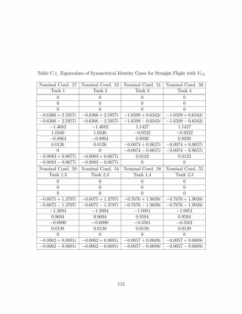
Table C.1. Eigenvalues of Symmetrical Identity Cases for Straight Flight with VT,2
Nominal Cond. 57 Nominal Cond. 53 Nominal Cond. 51 Nominal Cond. 50Tank 1 Tank 2 Tank 3 Tank 4
0 0 0 00 0 0 00 0 0 0
−0.6366 + 2.5957i −0.6366 + 2.5957i −1.6509 + 0.6342i −1.6509 + 0.6342i−0.6366− 2.5957i −0.6366− 2.5957i −1.6509− 0.6342i −1.6509− 0.6342i
−1.4682 −1.4682 1.1427 1.14271.0340 1.0340 −0.9522 −0.9522−0.8964 −0.8964 0.8030 0.80300.0126 0.0126 −0.0074 + 0.0657i −0.0074 + 0.0657i
0 0 −0.0074− 0.0657i −0.0074− 0.0657i−0.0083 + 0.0677i −0.0083 + 0.0677i 0.0123 0.0123−0.0083− 0.0677i −0.0083− 0.0677i 0 0
Nominal Cond. 59 Nominal Cond. 54 Nominal Cond. 58 Nominal Cond. 55Tank 1,3 Tank 2,4 Tank 1,4 Tank 2,3
0 0 0 00 0 0 00 0 0 0
−0.6075 + 1.3797i −0.6075 + 1.3797i −0.7676 + 1.9039i −0.7676 + 1.9039i−0.6075− 1.3797i −0.6075− 1.3797i −0.7676− 1.9039i −0.7676− 1.9039i
−1.2094 −1.2094 −1.0951 −1.09510.9694 0.9694 0.9594 0.9594−0.6990 −0.6990 −0.3501 −0.35010.0138 0.0138 0.0139 0.0139
0 0 0 0−0.0062 + 0.0691i −0.0062 + 0.0691i −0.0057 + 0.0689i −0.0057 + 0.0689i−0.0062− 0.0691i −0.0062− 0.0691i −0.0057− 0.0689i −0.0057− 0.0689i
115

Table C.2. Eigenvalues of Symmetrical Identity Cases for Straight Flight with VT,2
Nominal Cond. 63 Nominal Cond. 62 Nominal Cond. 60 Nominal Cond. 56Tank 1,2,3 Tank 1,2,4 Tank 1,3,4 Tank 2,3,4
0 0 0 00 0 0 00 0 0 0
−0.6551 + 2.6303i −0.6551 + 2.6303i −1.9158 −1.9158−0.6551− 2.6303i −0.6551− 2.6303i −1.0038 −1.0038
−1.0198 −1.0198 0.8199 + 0.0817i 0.8199 + 0.0817i0.8897 0.8897 0.8199− 0.0817i 0.8199− 0.0817i−0.4200 −0.4200 −0.2945 −0.29450.0157 0.0157 0.0152 0.0152
0 0 0 0−0.0063 + 0.0680i −0.0063 + 0.0680i −0.0058 + 0.0630i −0.0058 + 0.0630i−0.0063− 0.0680i −0.0063− 0.0680i −0.0058− 0.0630i −0.0058− 0.0630i
116

Table C.3. Eigenvalues of Symmetrical Identity Cases for Straight Flight with VT,1
Nominal Cond. 41 Nominal Cond. 37 Nominal Cond. 35 Nominal Cond. 34Tank 1 Tank 2 Tank 3 Tank 4
0 0 0 00 0 0 00 0 0 0
−0.5916 + 2.4109i −0.5916 + 2.4109i −1.5218 + 0.5860i −1.5218 + 0.5860i−0.5916− 2.4109i −0.5916− 2.4109i −1.5218− 0.5860i −1.5218− 0.5860i
−1.3206 −1.3206 1.0551 1.05510.9320 0.9320 −0.8902 −0.8902−0.8527 −0.8520 0.7298 0.72980.0150 0.0150 0.0146 0.0146
0 0 0 0−0.0081 + 0.0726i −0.0081 + 0.0726i −0.0074 + 0.0714i −0.0074 + 0.0714i−0.0081− 0.0726i −0.0081− 0.0726i −0.0074− 0.0714i −0.0074− 0.0714i
Nominal Cond. 43 Nominal Cond. 38 Nominal Cond. 42 Nominal Cond. 39Tank 1,3 Tank 2,4 Tank 1,4 Tank 2,3
0 0 0 00 0 0 00 0 0 0
−0.5655 + 1.2815i −0.5655 + 1.2815i −0.7134 + 1.7718i −0.7134 + 1.7718i−0.5655− 1.2815i −0.5655− 1.2815i −0.7134− 1.7718i −0.7134− 1.7718i
−1.0842 −1.0842 −0.9992 −0.99920.8732 0.8732 0.8677 0.8677−0.6652 −0.6652 −0.3254 −0.32540.0166 0.0166 0.0167 0.0167
0 0 0 0−0.0060 + 0.0738i −0.0060 + 0.0738i −0.0054 + 0.0736i −0.0054 + 0.0736i−0.0060− 0.0738i −0.0060− 0.0738i −0.0054− 0.0736i −0.0054− 0.0736i
117
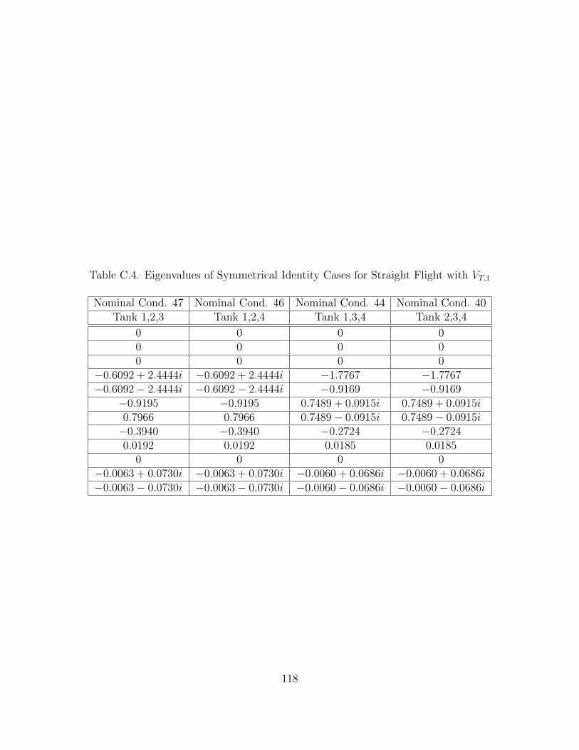
Table C.4. Eigenvalues of Symmetrical Identity Cases for Straight Flight with VT,1
Nominal Cond. 47 Nominal Cond. 46 Nominal Cond. 44 Nominal Cond. 40Tank 1,2,3 Tank 1,2,4 Tank 1,3,4 Tank 2,3,4
0 0 0 00 0 0 00 0 0 0
−0.6092 + 2.4444i −0.6092 + 2.4444i −1.7767 −1.7767−0.6092− 2.4444i −0.6092− 2.4444i −0.9169 −0.9169
−0.9195 −0.9195 0.7489 + 0.0915i 0.7489 + 0.0915i0.7966 0.7966 0.7489− 0.0915i 0.7489− 0.0915i−0.3940 −0.3940 −0.2724 −0.27240.0192 0.0192 0.0185 0.0185
0 0 0 0−0.0063 + 0.0730i −0.0063 + 0.0730i −0.0060 + 0.0686i −0.0060 + 0.0686i−0.0063− 0.0730i −0.0063− 0.0730i −0.0060− 0.0686i −0.0060− 0.0686i
118

APPENDIX D
TURNING FLIGHT EIGENVALUES COMPARISON
119

Table D.1. Eigenvalues of Turning Flight with VT,2
Nominal Cond. 89 Nominal Cond. 21 Nominal Cond. 85 Nominal Cond. 25Tank 1 Tank 2 Tank 2 Tank 1
ψT,2 = 1.7 ψT,3 = −1.7 ψT,2 = 1.7 ψT,3 = −1.7
−0.6348 + 2.5938i −0.6348 + 2.5938i −0.6356 + 2.5934i −0.6356 + 2.5934i−0.6348− 2.5938i −0.6348− 2.5938i −0.6356− 2.5934i −0.6356− 2.5934i
−1.3600 −1.3600 −1.3600 −1.36001.0141 1.0141 1.0130 1.0130−0.9884 −0.9884 −0.9870 −0.9870−0.0872 −0.0872 0.0820 0.0820
0.0407 + 0.0951i 0.0407 + 0.0951i −0.0423 + 0.1034i −0.0423 + 0.1034i0.0407− 0.0951i 0.0407− 0.0951i −0.0423− 0.1034i −0.0423− 0.1034i
+0.0297i +0.0297i +0.0297i +0.0297i−0.0297i −0.0297i −0.0297i −0.0297i
0 0 0 00 0 0 0
Nominal Cond. 83 Nominal Cond. 18 Nominal Cond. 82 Nominal Cond. 19Tank 3 Tank 4 Tank 4 Tank 3
ψT,2 = 1.7 ψT,3 = −1.7 ψT,2 = 1.7 ψT,3 = −1.7
−1.6186 + 0.6284i −1.6186 + 0.6284i −1.6184 + 0.6367i −1.6184 + 0.6367i−1.6186− 0.6284i −1.6186− 0.6284i −1.6184− 0.6367i −1.6184− 0.6367i
1.1326 1.1326 1.1343 1.1343−1.0024 −1.0024 −1.0102 −1.01020.7985 0.7985 0.7990 0.7990−0.0742 −0.0742 0.0817 0.0817
0.0353 + 0.0945i 0.0353 + 0.0945i −0.0402 + 0.0919i −0.0402 + 0.0919i0.0353− 0.0945i 0.0353− 0.0945i −0.0402− 0.0919i −0.0402− 0.0919i
+0.0297i +0.0297i +0.0297i +0.0297i−0.0297i −0.0297i −0.0297i −0.0297i
0 0 0 00 0 0 0
120

Table D.2. Eigenvalues of Turning Flight with VT,2
Nominal Cond. 93 Nominal Cond. 29 Nominal Cond. 91 Nominal Cond. 22Tank 1,2 Tank 1,2 Tank 1,3 Tank 2,4
ψT,2 = 1.7 ψT,3 = −1.7 ψT,2 = 1.7 ψT,3 = −1.7
−0.7041 + 3.4165i −0.7041 + 3.4165i −0.6032 + 1.3790i −0.6032 + 1.3790i−0.7041− 3.4165i −0.7041− 3.4165i −0.6032− 1.3790i −0.6032− 1.3790i
−1.0258 −1.0258 −1.1007 −1.10070.9339 0.9339 0.9514 0.9514−0.7618 −0.7618 −0.7918 −0.7918
−0.0066 + 0.0678i −0.0066 + 0.0678i −0.1469 −0.1469−0.0066− 0.0678i −0.0066− 0.0678i 0.0700 + 0.1216i 0.0700 + 0.1216i
0.0098 0.0098 0.0700− 0.1216i 0.0700− 0.1216i+0.0297i +0.0297i 0 +0.0297i−0.0297i −0.0297i +0.0297i −0.0297i
0 0 −0.0297i 00 0 0 0
Nominal Cond. 90 Nominal Cond. 23 Nominal Cond. 87 Nominal Cond. 26Tank 1,4 Tank 2,3 Tank 2,3 Tank 1,4
ψT,2 = 1.7 ψT,3 = −1.7 ψT,2 = 1.7 ψT,3 = −1.7
−0.7692 + 1.9069i −0.7692 + 1.9069i −0.7684 + 1.9067i −0.7684 + 1.9067i−0.7692− 1.9069i −0.7692− 1.9069i −0.7684− 1.9067i −0.7684− 1.9067i
−1.0523 −1.0523 −1.0536 −1.05360.9447 0.9447 0.9436 0.9436−0.3796 −0.3796 −0.3648 −0.36480.0720 0.0720 −0.0909 −0.0909
−0.0334 + 0.1066i −0.0334 + 0.1066i 0.0411 + 0.0879i 0.0411 + 0.0879i−0.0334− 0.1066i −0.0334− 0.1066i 0.0411− 0.0879i 0.0411− 0.0879i
+0.0297i +0.0297i +0.0297i +0.0297i−0.0297i −0.0297i −0.0297i −0.0297i
0 0 0 00 0 0 0
121

Table D.3. Eigenvalues of Turning Flight with VT,2
Nominal Cond. 86 Nominal Cond. 27 Nominal Cond. 84 Nominal Cond. 20Tank 2,4 Tank 1,3 Tank 3,4 Tank 3,4
ψT,2 = 1.7 ψT,3 = −1.7 ψT,2 = 1.7 ψT,3 = −1.7
−0.6114 + 1.3771i −0.6114 + 1.3771i −3.0003 −3.0003−0.6114− 1.3771i −0.6114− 1.3771i 1.9493 1.9493
−1.0967 −1.0967 −1.0980 −1.09800.9513 0.9513 0.9469 0.9469−0.7933 −0.7933 −0.4875 −0.48750.1216 0.1216 −0.0039 + 0.0671i −0.0039 + 0.0671i
−0.0572 + 0.1460i −0.0572 + 0.1460i −0.0039− 0.0671i −0.0039− 0.0671i−0.0572− 0.1460i −0.0572− 0.1460i 0.0075 0.0075
+0.0297i +0.0297i +0.0297i +0.0297i−0.0297i −0.0297i −0.0297i −0.0297i
0 0 0 00 0 0 0
Nominal Cond. 92 Nominal Cond. 24 Nominal Cond. 88 Nominal Cond. 28Tank 1,3,4 Tank 2,3,4 Tank 2,3,4 Tank 1,3,4
ψT,2 = 1.7 ψT,3 = −1.7 ψT,2 = 1.7 ψT,3 = −1.7
−1.9090 −1.9090 −1.9079 −1.9079−0.9645 −0.9645 −0.9653 −0.9653
0.8110 + 0.0825i 0.8110 + 0.0825i −0.3206 −0.32060.8110− 0.0825i 0.8110− 0.0825i 0.8105 + 0.0798i 0.8105 + 0.0798i−0.3207 −0.3207 0.8105− 0.0798i 0.8105− 0.0798i0.0222 0.0222 −0.0218 −0.0218
−0.0114 + 0.0719i −0.0114 + 0.0719i 0.0110 + 0.0569i 0.0110 + 0.0569i−0.0114− 0.0719i −0.0114− 0.0719i 0.0110− 0.0569i 0.0110− 0.0569i
+0.0297i +0.0297i +0.0297i +0.0297i−0.0297i −0.0297i −0.0297i −0.0297i
0 0 0 00 0 0 0
122

Table D.4. Eigenvalues of Turning Flight with VT,2
Nominal Cond. 96 Nominal Cond. 32 Nominal Cond. 81 Nominal Cond. 17Tank 1,2,3,4 Tank 1,2,3,4 Tank empty Tank empty
ψT,2 = 1.7 ψT,3 = −1.7 ψT,2 = 1.7 ψT,3 = −1.7
−0.4805 + 1.4135i −0.4805 + 1.4135i −0.7649 + 1.4286i −0.7649 + 1.4286i−0.4805− 1.4135i −0.4805− 1.4135i −0.7649 + 1.4286i −0.7649 + 1.4286i
−0.8726 −0.8726 −1.6119 −1.61190.7955 0.7955 1.1162 1.1162−0.4182 −0.4182 −0.9428 −0.94280.0098 0.0098 −0.0072 + 0.0701i −0.0072 + 0.0701i
−0.0036 + 0.0708i −0.0036 + 0.0708i −0.0072− 0.0701i −0.0072− 0.0701i−0.0036− 0.0708i −0.0036− 0.0708i 0.0083 0.0083
+0.0297i +0.0297i +0.0297i +0.0297i−0.0297i −0.0297i −0.0297i −0.0297i
0 0 0 00 0 0 0
123
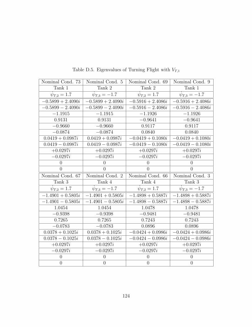
Table D.5. Eigenvalues of Turning Flight with VT,1
Nominal Cond. 73 Nominal Cond. 5 Nominal Cond. 69 Nominal Cond. 9Tank 1 Tank 2 Tank 2 Tank 1
ψT,2 = 1.7 ψT,3 = −1.7 ψT,2 = 1.7 ψT,3 = −1.7
−0.5899 + 2.4090i −0.5899 + 2.4090i −0.5916 + 2.4086i −0.5916 + 2.4086i−0.5899− 2.4090i −0.5899− 2.4090i −0.5916− 2.4086i −0.5916− 2.4086i
−1.1915 −1.1915 −1.1926 −1.19260.9131 0.9131 −0.9641 −0.9641−0.9660 −0.9660 0.9117 0.9117−0.0874 −0.0874 0.0840 0.0840
0.0419 + 0.0987i 0.0419 + 0.0987i −0.0419 + 0.1080i −0.0419 + 0.1080i0.0419− 0.0987i 0.0419− 0.0987i −0.0419− 0.1080i −0.0419− 0.1080i
+0.0297i +0.0297i +0.0297i +0.0297i−0.0297i −0.0297i −0.0297i −0.0297i
0 0 0 00 0 0 0
Nominal Cond. 67 Nominal Cond. 2 Nominal Cond. 66 Nominal Cond. 3Tank 3 Tank 4 Tank 4 Tank 3
ψT,2 = 1.7 ψT,3 = −1.7 ψT,2 = 1.7 ψT,3 = −1.7
−1.4901 + 0.5805i −1.4901 + 0.5805i −1.4898 + 0.5887i −1.4898 + 0.5887i−1.4901− 0.5805i −1.4901− 0.5805i −1.4898− 0.5887i −1.4898− 0.5887i
1.0454 1.0454 1.0478 1.0478−0.9398 −0.9398 −0.9481 −0.94810.7265 0.7265 0.7243 0.7243−0.0783 −0.0783 0.0896 0.0896
0.0378 + 0.1025i 0.0378 + 0.1025i −0.0424 + 0.0986i −0.0424 + 0.0986i0.0378− 0.1025i 0.0378− 0.1025i −0.0424− 0.0986i −0.0424− 0.0986i
+0.0297i +0.0297i +0.0297i +0.0297i−0.0297i −0.0297i −0.0297i −0.0297i
0 0 0 00 0 0 0
124

Table D.6. Eigenvalues of Turning Flight with VT,1
Nominal Cond. 77 Nominal Cond. 13 Nominal Cond. 75 Nominal Cond. 6Tank 1,2 Tank 1,2 Tank 1,3 Tank 2,4
ψT,2 = 1.7 ψT,3 = −1.7 ψT,2 = 1.7 ψT,3 = −1.7
−0.6548 + 3.1745i −0.6548 + 3.1745i −0.5616 + 1.2809i −0.5616 + 1.2809i−0.6548− 3.1745i −0.6548− 3.1745i −0.5616− 1.2809i −0.5616− 1.2809i
−0.8508 −0.8508 −0.9536 −0.95360.8332 0.8332 0.8561 0.8561−0.7806 −0.7806 −0.7785 −0.7785
−0.0065 + 0.0730i −0.0065 + 0.0730i −0.1503 −0.1503−0.0065− 0.0730i −0.0065− 0.0730i 0.0724 + 0.1241i 0.0724 + 0.1241i
0.0120 0.0120 0.0724− 0.1241i 0.0724− 0.1241i+0.0297i +0.0297i +0.0297i +0.0297i−0.0297i −0.0297i −0.0297i −0.0297i
0 0 0 00 0 0 0
Nominal Cond. 74 Nominal Cond. 7 Nominal Cond. 71 Nominal Cond. 10Tank 1,4 Tank 2,3 Tank 2,3 Tank 1,4
ψT,2 = 1.7 ψT,3 = −1.7 ψT,2 = 1.7 ψT,3 = −1.7
−0.7148 + 1.7744i −0.7148 + 1.7744i −0.7142 + 1.7743i −0.7142 + 1.7743i−0.7148− 1.7744i −0.7148− 1.7744i −0.7142− 1.7743i −0.7142− 1.7743i
−0.9573 −0.9573 −0.9591 −0.95910.8541 0.8541 0.8521 0.8527−0.3564 −0.3564 −0.3370 −0.33700.0725 0.0725 −0.0924 −0.0924
−0.0316 + 0.1112i −0.0316 + 0.1112i 0.0421 + 0.0901i 0.0421 + 0.0901i−0.0316− 0.1112i −0.0316− 0.1112i 0.0421− 0.0901i 0.0421− 0.0901i
+0.0297i +0.0297i +0.0297i +0.0297i−0.0297i −0.0297i −0.0297i −0.0297i
0 0 0 00 0 0 0
125
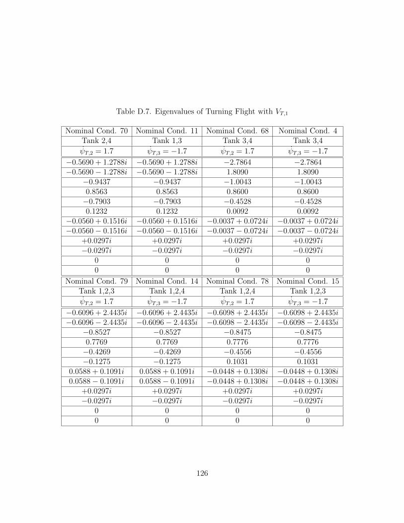
Table D.7. Eigenvalues of Turning Flight with VT,1
Nominal Cond. 70 Nominal Cond. 11 Nominal Cond. 68 Nominal Cond. 4Tank 2,4 Tank 1,3 Tank 3,4 Tank 3,4
ψT,2 = 1.7 ψT,3 = −1.7 ψT,2 = 1.7 ψT,3 = −1.7
−0.5690 + 1.2788i −0.5690 + 1.2788i −2.7864 −2.7864−0.5690− 1.2788i −0.5690− 1.2788i 1.8090 1.8090
−0.9437 −0.9437 −1.0043 −1.00430.8563 0.8563 0.8600 0.8600−0.7903 −0.7903 −0.4528 −0.45280.1232 0.1232 0.0092 0.0092
−0.0560 + 0.1516i −0.0560 + 0.1516i −0.0037 + 0.0724i −0.0037 + 0.0724i−0.0560− 0.1516i −0.0560− 0.1516i −0.0037− 0.0724i −0.0037− 0.0724i
+0.0297i +0.0297i +0.0297i +0.0297i−0.0297i −0.0297i −0.0297i −0.0297i
0 0 0 00 0 0 0
Nominal Cond. 79 Nominal Cond. 14 Nominal Cond. 78 Nominal Cond. 15Tank 1,2,3 Tank 1,2,4 Tank 1,2,4 Tank 1,2,3
ψT,2 = 1.7 ψT,3 = −1.7 ψT,2 = 1.7 ψT,3 = −1.7
−0.6096 + 2.4435i −0.6096 + 2.4435i −0.6098 + 2.4435i −0.6098 + 2.4435i−0.6096− 2.4435i −0.6096− 2.4435i −0.6098− 2.4435i −0.6098− 2.4435i
−0.8527 −0.8527 −0.8475 −0.84750.7769 0.7769 0.7776 0.7776−0.4269 −0.4269 −0.4556 −0.4556−0.1275 −0.1275 0.1031 0.1031
0.0588 + 0.1091i 0.0588 + 0.1091i −0.0448 + 0.1308i −0.0448 + 0.1308i0.0588− 0.1091i 0.0588− 0.1091i −0.0448 + 0.1308i −0.0448 + 0.1308i
+0.0297i +0.0297i +0.0297i +0.0297i−0.0297i −0.0297i −0.0297i −0.0297i
0 0 0 00 0 0 0
126

Table D.8. Eigenvalues of Turning Flight with VT,1
Nominal Cond. 76 Nominal Cond. 8 Nominal Cond. 72 Nominal Cond. 12Tank 1,3,4 Tank 2,3,4 Tank 2,3,4 Tank 1,3,4
ψT,2 = 1.7 ψT,3 = −1.7 ψT,2 = 1.7 ψT,3 = −1.7
−1.7700 −1.7700 −1.7691 −1.7691−0.8783 −0.8783 −0.8794 −0.8794
0.7407 + 0.0919i 0.7407 + 0.0919i 0.7393 + 0.0882i 0.7393 + 0.0882i0.7407− 0.0919i 0.7407− 0.0919i 0.7393− 0.0882i 0.7393− 0.0882i−0.2978 −0.2978 −0.2977 −0.2977
−0.0044 + 0.0751i −0.0044 + 0.0751i −0.0006 + 0.0588i −0.0006 + 0.0588i−0.0044− 0.0751i −0.0044− 0.0751i −0.0006− 0.0588i −0.0006− 0.0588i
0.0095 0.0095 0.0045 0.00450 0 +0.0297i +0.0297i0 0 −0.0297i −0.0297i
+0.0297i +0.0297i 0 0−0.0297i −0.0297i 0 0
Nominal Cond. 80 Nominal Cond. 16 Nominal Cond. 65 Nominal Cond. 1Tank 1,2,3,4 Tank 1,2,3,4 Tank empty Tank empty
ψT,2 = 1.7 ψT,3 = −1.7 ψT,2 = 1.7 ψT,3 = −1.7
−0.4470 + 1.3133i −0.4470 + 1.3133i −0.7114 + 1.3278i −0.7114 + 1.3278i−0.4470− 1.3133i −0.4470− 1.3133i −0.7114− 1.3278i −0.7114− 1.3278i
−0.7807 −0.7807 −1.4681 −1.46810.7097 0.7097 1.0143 1.0143−0.3947 −0.3947 −0.8861 −0.88610.0124 0.0124 −0.0065 + 0.0747i −0.0065 + 0.0747i
−0.0033 + 0.0760i −0.0033 + 0.0760i −0.0065− 0.0747i −0.0065− 0.0747i−0.0033− 0.0760i −0.0033− 0.0760i 0.0097 0.0097
+0.0297i +0.0297i +0.0297i +0.0297i−0.0297i −0.0297i −0.0297i −0.0297i
0 0 0 00 0 0 0
127

REFERENCES
[1] J. J. Kim and B. N. Agrawal, “System identification and automatic mass bal-
ancing of ground-based three-axis spacecraft simulator,” in Proc. of the AIAA
Guidance, Navigation and Control Conference and Exhibit, Keystone, CO, 2006,
p. 6595.
[2] ——, “Automatic mass balancing of air-bearing-based three-axis rotational
spacecraft simulator,” AIAA Journal of Guidance, Control, and Dynamics,
vol. 32, no. 3, pp. 1005–1017, 2009.
[3] M. Abraham and M. Costello, “In-flight estimation of helicopter gross weight
and mass center location,” Journal of Aircraft, vol. 46, pp. 1042–1049, 1995.
[4] Y. Bestaoui, “A lagrangian approach to modeling of an airship with wind and
varying mass effects,” in Proc. of 48th AIAA Aerospace Sciences Meeting includ-
ing the New Horizons Forum and Aerospace Exposition, Orlando, Florida, 4-7
January 2010, p. 40.
[5] L. Chen and G. Zhou and X. J. Yan and D. P. Duan, “Composite control strategy
of stratospheric airships with moving masses,” AIAA Journal of Aircraft, vol. 49,
no. 3, pp. 794–801, May-June 2012.
[6] P. Lin and J. Zhou, “Researching variable structure control of moving mass
reentry-vehicles,” in Proc. of the IEEE International Conference on Computer
Science and Information Technology, Chengdu, China, 9-11 July 2010, pp. 126–
129.
128
[7] Matt R. Jardin and Eric R. Mueller, “Optimized measurements of unmanned-
air-vehicle mass moment of inertia with a bifilar pendulum,” AIAA Journal of
Aircraft, vol. 46, no. 3, pp. 763–775, May-June 2009.
[8] K. D. Kumar and A.-M. Zou, “Attitude control of miniature satellite using mov-
able masses,” in Proc. of AIAA SpaceOps Conference Delivering on the Dream
Hosted by NASA Mars, Huntsville, Alabama, 25-31 April 2010, p. 1982.
[9] P. K. Menon and G. D. Sweriduk and E. J. Ohlmeyer and D. S. Malyevac,
“Integrated guidance and control of moving-mass actuated kinetic warheads,”
AIAA Journal of Guidance, Control, and Dynamics, vol. 27, no. 1, pp. 118–126,
January-February 2004.
[10] P. K. Menon and S. S. Vaddi, “Finite-horizon robust integrated guidance-control
of a moving-mass actuated kinetic warhead,” in Proc. of AIAA Guidance, Nav-
igation, and Control Conference and Exhibit, Keystone, Colorado, 21-24 August
2006, p. 6787.
[11] Rudranarayan M. Mukherjee and J. (Bob) Balaram, “Attitude dynamics and
control of moving mass multibody aeromaneuver vehicle,” in Proc. of AIAA
Atmospheric Flight Mechanics Conference and Exhibit, Honolulu, Hawaii, 18-21
August 2008, p. 6390.
[12] Y. Qianchen, Z. Qingzhen, and Z. Huiping, “A compound control system of axial
moving mass and aerodynamic force for mass moment missile,” in Proc. of the
IEEE International Conference on Instrumentation, Measurement, Computer,
Communication and Control, Beijing, China, 21-23 October 2011, pp. 945–948.
[13] L. Qin and M. Yang, “Moving mass attitude law based on neural networks.”
[14] J. Rogers and M. Costello, “Flight dynamics and control authority of a projectile
equipped with a controllable internal translating mass,” in Proc. of AIAA Atmo-
129

spheric Flight Mechanics Conference and Exhibit, Hilton Head, South Carolina,
20-23 August 2007, p. 6492.
[15] ——, “A variable stability projectile using an internal moving mass,” in Proc. of
AIAA Atmospheric Flight Mechanics Conference and Exhibit, Honolulu, Hawaii,
18-21 August 2008, p. 7116.
[16] ——, “Control authority of a projectile equipped with a controllable internal
translating mass,” AIAA Journal of Guidance, Control, and Dynamics, vol. 31,
no. 5, pp. 1323–1333, September-October 2008.
[17] D. Wang, J. S. Jiang, and W. H. Zhang, “Frequency optimization with respect to
lumped mass position,” AIAA Journal, vol. 41, no. 9, pp. 1780–1787, September
2003.
[18] S. Wang, M. Yang, and Z. Wang, “Moving-mass trim control system design for
spinning vehicles.”
[19] C. A. Woolsey and N. E. Leonard, “Moving mass control for underwater vehi-
cles.”
[20] Y. Jiang, F. He, and Y. Yao, “Hybrid control strategy for attitude stabilization
of an underactuated spacecraft with two moving mass,” in Proc. of the IEEE In-
ternational Conference on Automation and Logistics, Jinan, China, 18-21 August
2007, pp. 389–393.
[21] P. K. Menon and S. S. Vaddi, “Finite-horizon robust integrated guidance-control
of a moving-mass actuated kinetic warhead,” in Proc. of AIAA Guidance, Nav-
igation, and Control Conference and Exhibit, Keystone, Colorado, 21-24 August
2006, p. 6787.
[22] R. H. Byrne, B. R. Sturgis, and R. D. Robinett, “A moving mass trim con-
trol system for reentry vehicle guidance,” in Proc. of AIAA Atmospheric Flight
Mechanics Conference, San Diego, California, 29-31 July 1996, p. 3438.
130

[23] R. H. Byrne, R. D. Robinett, and B. R. Sturgis, “Moving mass trim control
system design,” in Proc. of AIAA Guidance, Navigation and Control Conference,
San Diego, California, 29-31 July 1996, p. 3826.
[24] W. Okolo, A. Dogan, and W. Blake, “Aircraft lateral trim using internal fuel
transfer and differential thrust in formation flight,” in Proc. of the AIAA Atmo-
spheric Flight Mechanics Conference, Portland, Oregon, 08-11 August 2011, p.
6613.
[25] C. S. Beaverstock, J. Fincham, M. I. Friswell, R. M. Ajaj, R. D. Breuker, and
N. Werter, “Effect of symmetric and asymmetric span morphing on flight dynam-
ics,” in Proc. of the AIAA Atmospheric Flight Mechanics Conference, National
Harbor, Maryland, 13-17 January 2014, p. 0545.
[26] Jayme Waiskek and Atilla Dogan and William Blake, “Derivation of the dynam-
ics equations of receiver aircraft in aerial refueling,” AIAA Journal of Guidance,
Control, and Dynamics, vol. 32, no. 2, pp. 585–597, March-April 2009.
[27] M.-G. Yoon, V. A. Ugrinovskii, and M. Pszczel, “Gain-scheduling of minimax op-
timal state-feedback controllers for uncertain linear parameter-varying systems.”
[28] D. Saussie, L. Saydy, O. Akhrif, and C. Berard, “Gain scheduling with guardian
maps for longitudinal flight control,” Journal of Guidance, Control, and Dynam-
ics, vol. 34, no. 4, pp. 1045–1059, July-August 2011.
[29] D. Saussie, L. Saydy, and O. Akhrif, “Gain scheduling control design for a pitch-
axis missile autopilot,” in Proc. of the AIAA Guidance, Navigation and Control
Conference and Exhibit, Honolulu, Hawaii, August 2008, p. 7000.
[30] Y. Hamada, T. Ohtani, T. Kida, and T. Nagashio, “Synthesis of a linearly inter-
polated gain scheduling controller for large flexible spacecraft ets-viii,” Control
Engineering Practice, vol. 19, no. 6, pp. 611–625, June 2011.
131

[31] S. Theodoulis and G. Duc., “Missile autopilot design: Gain-scheduling and the
gap metric,” Journal of Guidance, Control, and Dynamics, vol. 32, no. 3, pp.
986–996, May-June 2009.
[32] J. YU, G. LUO, and Y. MEI, “Surface-to-air missile autopilot design using lqg/ltr
gain scheduling method,” Chinese Journal of Aeronautics, vol. 24, no. 3, pp. 279–
286, June 2011.
[33] S. McNamara, C. Restrepo, E. Medina, R. Whitley, R. Proud, and J. Madsen,
“Gain scheduling for the orion launch abort vehicle controller,” in Proc. of the
AIAA Guidance, Navigation and Control Conference, Portland, Oregon, 08-11
August 2011, p. 6259.
[34] W. Yang, M. N. Hammoudi, G. Herrmann, M. Lowenberg, and X. Chen, “Two-
state dynamic gain scheduling control applied to an f16 aircraft model,” In-
ternational Journal of Non-Linear Mechanics, vol. 47, no. 10, pp. 1116–1123,
December 2012.
[35] R. Smith and A. Ahmed, “Robust parametrically varying attitude controller
designs for the x-33 vehicle,” in Proc. of the AIAA Guidance, Navigation, and
Control Conference, Denver, Colorado, 14-17 August 2000, p. 4158.
[36] G.-H. Yang and K.-Y. Lum, “Gain-scheduled flight control via state feedback,” in
Proc. of the American Control Conference, Denver, Colorado, 04-06 June 2003,
pp. 3484–3489.
[37] D. P. White, J. G. Wozniak, and D. A. Lawrence, “Missile autopilot design using
a gain scheduling technique.”
[38] A. Fujimori, Z. Wu, P. N. Nikiforuk, and M. M. Gupta, “A design of a flight
control system using fuzzy gain-scheduling,” in Proc. of the AIAA Guidance,
Navigation and Control Conference, New Orleans, Louisiana, August 1997, p.
3760.
132

[39] C. D. C. Jones, M. H. Lowenberg, and T. S. Richardson, “Tailored dynamic
gain-scheduled control,” Journal of Guidance, Control, and Dynamics, vol. 29,
no. 6, pp. 1271–1281, November-December 2006.
[40] B. CLEMENT and G. DUC, “An interpolation method for gain-scheduling,”
in Proc. of the IEEE the 40th Conference on Decision and Control, Orlando,
Florida, December 2001, pp. 1310–1315.
[41] Pierre Apkarian and Richard J. Adams, “Advanced gain-scheduling techniques
for uncertain systems,” IEEE Transactions on Control Systems Technology,
vol. 6, no. 1, pp. 21–32, January 1998.
[42] Jianying Gao and Hector M. Budman, “Design of robust gain-scheduled pi con-
trollers for nonlinear processes,” Journal of Process Control, vol. 15, no. 7, pp.
807–817, October 2005.
[43] S. Alepuz, J. Bordonau, and J. Peracaula, “A novel control approach of three-
level vsis using a lqr-based gain-scheduling technique.”
[44] Isaac Kaminer and Antonio M. Pascoal and Pramod P. Khargonekar and Edward
E. Coleman, “A velocity algorithm for the implementation of gain-scheduled
controllers,” Automatica, vol. 31, no. 8, pp. 1185–1191, August 1995.
[45] D. A. Lawrence and W. J. Rugh, “Gain scheduling dynamic linear controllers,”
Automatica, vol. 31, no. 3, pp. 381–390, March 1995.
[46] Daniel J. Stilwell and Douglas A. Lawrence, “Sampled-data implementation of a
gain scheduled controller,” International Journal of Robust and Nonlinear Con-
trol, vol. 12, no. 9, pp. 855–868, July 2002.
[47] J. S. Shamma and M. Athans, “Gain scheduling: Potential hazards and possible
remedies,” IEEE Control Systems, vol. 12, no. 3, pp. 101–107, June 1992.
[48] ——, “Analysis of gain scheduled control for nonlinear plants,” IEEE Transac-
tions on Automatic Control, vol. 35, no. 8, pp. 898–907, August 1990.
133

[49] F. J. D. III, H. S. Kwatra, and J. S. Schwaber, “Dynamic gain scheduled process
control,” Chemical Engineering Science, vol. 53, no. 15, pp. 2675–2690, August
1998.
[50] S. R. Wells and R. A. Hess, “Multi-input/multi-output sliding mode control for
a tailless fighter aircraft,” AIAA Journal of Guidance, Control, and Dynamics,
vol. 26, no. 3, pp. 463–473, May-June 2003.
[51] Gao C. and Hess R.A., “Inverse simulation of large amplitude aircraft maneu-
vers,” AIAA Journal of Guidance,Control,Dynamic, vol. 16, no. 4, pp. 733–737,
July 1993.
[52] F. Blanchini, “The gain scheduling and the robust state feedback stabilization
problems,” IEEE Transactions on Automatic Control, vol. 45, no. 11, pp. 2061–
2070, November 2000.
[53] Eunyoung Kim, “Control and simulation of relative motion for aerial refueling
in racetrack maneuver,” Master’s thesis, The University of Texas at Arlington,
May 2007.
[54] Austin L. Smith and Donalad L. Kunz, “Dynamic coupling of the kc 135 tanker
and boom for modeling and simulation,” AIAA Journal of Aircraft, vol. 44, no. 3,
pp. 1034–1039, May-June 2007.
[55] D. K.-J. Jackson, C. Tyler, and W. B. Blake, “Computational analysis of air-
to-air refueling,” in Proc. of the 25th AIAA Applied Aerodynamics Conference,
Miami, Florida, 25-28 June 2007, p. 4289.
[56] A. F. Barfield and J. L. Hinchman, “An equivalent model for uav automated
aerial refueling research,” in Proc. of the AIAA Modeling and Simulation Tech-
nologies Conference and Exhibit, San Francisco, California, 15-18 August 2005,
p. 6006.
134

BIOGRAPHICAL STATEMENT
EunYoung Kim was born in Seoul, Korea. She came to the U.S to join the
university program in 2000 and pursued a bachelors degree in aerospace engineering
with computer science as a double major at Iowa State University. After graduating
from ISU in spring 2005, she joined the aerospace engineering graduate program
at the University of Texas at Arlington in August 2005. While she worked on the
Computer Aided Control Systems Design Lab with Dr. Atilla Dogan, she published
a paper entitled Control of a Receiver Aircraft Relative to the Tanker in Racetrack
Maneuver to the American Institute of Aeronautics and Astronautics (AIAA) in
August 2006, and ”Control of Simulation of Relative Motion for Aerial Refueling in
Racetrack Maneuvers” to the Journal of Guidance, Control, and Dynamics (AIAA) in
2007. For her Master Thesis she published a paper entitled ”Control and Simulation
of Relative Motion for Aerial Refueling in Racetrack Maneuver” in May 2007. After
pursuing Master degree in Aerospace Engineering from UTA she was continuing study
in Doctoral program in Aerospace Engineering at UTA. After graduating from UTA
she will go back to Korea and pursue fulltime research in the aerospace field.
135