Embed Size (px)
Citation preview

CRANFIELD UNIVERSITY
WEI GUO
GAIN SCHEDULING FOR A PASSENGER
AIRCRAFT CONTROL SYSTEM TO SATISFY
HANDLING QUALITIES
SCHOOL OF ENGINEERING
MSc BY RESEARCH THESIS
December 2010

This page intentionally contains only this sentence.

CRANFIELD UNIVERSITY
SCHOOL OF ENGINEERING
MSc BY RESEARCH THESIS
Academic Year 2010-11
WEI GUO
GAIN SCHEDULING FOR A PASSENGER AIRCRAFT
CONTROL SYSTEM TO SATISFY HANDLING
QUALITIES
Supervisor: Dr. James F. Whidborne
December 2010
c©Cranfield University 2010. All rights reserved. No part of this publication maybe reproduced without the written permission of the copyright owner.

This page intentionally contains only this sentence.
i
Abstract
This thesis considers the problem of designing gain scheduled flight control system(FCS) for large transport aircraft that satisfy handling qualities criteria. The goal isto design a set of local Linear Time Invariant (LTI) controllers to cover the wide non-linear aircraft operation flight envelope from the viewpoint of the handling qualitiesassessment. The global gain scheduler is then designed that interpolates betweenthe gains of the local controllers in order to transfer smoothly between differentequilibrium points, and more importantly to satisfy the handling qualities over theentire flight envelope. The mathematical model of the Boeing 747-100/200 aircraftis selected for the purpose of the flight controller design and handling qualities as-sessment.
In order to achieve an attitude hold characteristic, and also improve the dynamictracking behavior of the aircraft, longitudinal pitch Rate Command-Attitude Hold(RCAH) controllers are designed as the local flight controllers at the specific equilib-rium points in the flight envelope by means of a state space pole placement designprocedure.
The handling qualities assessment of the aircraft is presented, based on which thescheduler is designed. A number of existing criteria are employed to assess the han-dling qualities of the aircraft, including the Control Anticipation Parameter (CAP),Neal and Smith, and C∗ criteria. The gain scheduled flight controller is found tohave satisfactory handling qualities.
The global gain scheduler is designed by interpolating the gains of the local flightcontrollers in order to transfer smoothly between different equilibrium points, andmore importantly to satisfy the handling qualities over the flight envelope.
The main contribution of this research is the combination of the gain schedulingtechnique based on the local controller design approach and handling qualities as-sessment. The controllers are designed based at a number of operating points andthe interpolation between them (scheduling) takes place through the schedulingscheme functions. The aircraft augmented with gain-scheduled controller performssatisfactorily and meets the requirement of handling qualities. Moreover, the per-formance using the gain-scheduled controller is considerably improved compared tothe performance using the fixed one.
Keywords:Gain Scheduling, Flight Control System, Handling Qualities, Rate Command-AttitudeHold, Passenger Aircraft, Flight Dynamics, Boeing 747

This page intentionally contains only this sentence.

iii
Acknowledgements
Since the 3rd of January, 2010 (it was a snowy day just like today and the first dayof my studies abroad), it has been one year full of adventure, challenge, enjoyment,happiness and great experiences. I have been particularly fortunate during myresearch to have collaborated with a broad range of School of Engineering students.I would like to take this opportunity to acknowledge the help and support of a few.
I would like to express my sincerest gratitude to my supervisor, Dr. James Whid-borne for his continual advice, guidance, and support throughout the past year. Hiskeen insights and clear guidance gave me great encouragement to carry out thisresearch and made this thesis possible. I am also grateful to Dr. Alastair Cooke,Mr. Mike Cook and Dr. Thomas Richardson, who provided assistance and tech-nical support, and guided me with valuable suggestions during my studies. I amindebted to Dr. Al Savvaris and Dr. Bowen Zhong, whose knowledge and experi-ence was of great benefit to my time at Cranfield. My thanks also go to the otherpast and present members of the Dynamics, Simulation and Control group, espe-cially Sunan Chumalee, Stuart Andrews, Mudassir Lone, Peter Thomas, Ken Lai,Mohmad Rouyan Nurhana, Pierre-Daniel Jameson and Neil Panchal. They werealways open for discussions on my research struggles. Their friendship and sup-port also sustained me through many challenging occasions, and helped me to moveforward.
I would like to acknowledge China Scholarship Council (CSC), Commercial AircraftCorporation of China (COMAC), and COMAC’s subsidiary: Shanghai Aircraft De-sign and Research Institute (SADRI). My research and study would not have beenpossible without financial support from CSC and COMAC, and the nurturing en-vironment of SADRI. There are a number of people, family and friends that I amgrateful to and who deserve to be a part of every step forward that I have made.
Particular thanks go to the head of the Department of Flight Control System Designat SADRI, Jingzhou Zhao, who encouraged and believed in me ever since this projectwas first mentioned, and was continually supportive and attentive in my studies andwell being in the UK. All of these stimulated me enormously to greater efforts toavoid letting him down and made me carry the fight through to the end.
I am also grateful to the encouragement and a great comfort I derived from my othercolleagues of the COMAC group and Daqing Yang, who I fortunately collaborated

iv
and shared this studying abroad life with, and who were my companions endeavour-ing in a different field of aerospace side by side with me. Everything we have beenthrough together in the UK will be treasured deeply.
I would like to save my deepest gratitude to my family, without whose understanding,support and encouragement I would not have achieved even a little: to my parentsChonglun Guo and Yuezhi Lee, my sister Hui Guo and all my other family members.Their love is worth far more than any degree and I am very blessed to have themthere for me.
My time here at Cranfield has been memorable and valuable. I have enjoyed everyaspect of this country. Once again, I would like to thank, everybody who helped mefinish this research and made this Cranfield experience a most pleasant one.
Wei GuoJanuary, 2011

CONTENTS v
Contents
Contents v
List of figures ix
List of tables xii
Abbreviations xiii
Nomenclature xiv
1 Introduction 1
1.1 Background . . . . . . . . . . . . . . . . . . . . . . . . . . . . . . . . 1
1.2 Aim and Objectives . . . . . . . . . . . . . . . . . . . . . . . . . . . . 2
1.3 Summary . . . . . . . . . . . . . . . . . . . . . . . . . . . . . . . . . 4
2 Literature Review 5
2.1 Flight Control System . . . . . . . . . . . . . . . . . . . . . . . . . . 5
2.1.1 Functional Description . . . . . . . . . . . . . . . . . . . . . . 5
2.1.2 Command and Stability Augmentation System . . . . . . . . . 7
2.2 Gain Scheduling . . . . . . . . . . . . . . . . . . . . . . . . . . . . . . 9
2.3 Handling Qualities . . . . . . . . . . . . . . . . . . . . . . . . . . . . 13
3 Controller Design 15
3.1 Aircraft Model Introduction . . . . . . . . . . . . . . . . . . . . . . . 15

vi CONTENTS
3.2 Trim and Linearization . . . . . . . . . . . . . . . . . . . . . . . . . . 17
3.2.1 Aircraft Model Trim . . . . . . . . . . . . . . . . . . . . . . . 17
3.2.2 Aircraft Model Linearization . . . . . . . . . . . . . . . . . . . 18
3.3 Aircraft Equations of Motion . . . . . . . . . . . . . . . . . . . . . . 18
3.4 Design Requirements . . . . . . . . . . . . . . . . . . . . . . . . . . . 21
3.5 Controller Design . . . . . . . . . . . . . . . . . . . . . . . . . . . . . 23
3.5.1 Augmenting the Reduced Order Mode State Equation . . . . . 24
3.5.2 Designing the Gain Matrix K . . . . . . . . . . . . . . . . . . 25
3.5.3 Designing the Feedforward Gain Matrix M . . . . . . . . . . . 26
3.5.4 Implementing the Controller Design . . . . . . . . . . . . . . . 26
3.5.5 Checking the Design with the Full Order Aircraft Model . . . 27
4 Handling Qualities Assessment 31
4.1 The CAP Assessment . . . . . . . . . . . . . . . . . . . . . . . . . . . 31
4.2 The Neal and Smith Criterion Assessment . . . . . . . . . . . . . . . 33
4.3 The C∗ Criterion Assessment . . . . . . . . . . . . . . . . . . . . . . 34
5 Assessment over the Whole Flight Envelope 37
5.1 Introduction . . . . . . . . . . . . . . . . . . . . . . . . . . . . . . . . 37
5.2 Handling Qualities Assessment of Aircraft with C1 in F . . . . . . . . 38
5.2.1 Aircraft Models and the B747 flight envelope F . . . . . . . . 38
5.2.2 Identification of F1 . . . . . . . . . . . . . . . . . . . . . . . . 39
5.3 Controller(C2) Design for the Second Equilibrium Point EP(8500,180) . 43
5.4 Handling Qualities Assessment of C2 on EP(8500,180) . . . . . . . . . . 44
5.4.1 CAP . . . . . . . . . . . . . . . . . . . . . . . . . . . . . . . . 44
5.4.2 The Neal and Smith Criterion . . . . . . . . . . . . . . . . . 45
5.4.3 C∗ Criterion . . . . . . . . . . . . . . . . . . . . . . . . . . . . 46
5.5 Handling Qualities Assessment of Aircraft with C2 in F . . . . . . . . 47
5.6 Discussion of F1 and F2 . . . . . . . . . . . . . . . . . . . . . . . . . 47

CONTENTS vii
5.6.1 Analysis of Aircraft Model on EP(11500,210) Augmented by C2 . 48
5.6.2 Handling Assessment for C2 on EP(11500,210) . . . . . . . . . . 48
5.6.3 Summary . . . . . . . . . . . . . . . . . . . . . . . . . . . . . 48
5.7 Chapter-Summary . . . . . . . . . . . . . . . . . . . . . . . . . . . . 50
6 Gain Scheduling 59
6.1 Gain Scheduling Factor . . . . . . . . . . . . . . . . . . . . . . . . . . 59
6.2 Scheduled Gain Matrices . . . . . . . . . . . . . . . . . . . . . . . . . 60
6.2.1 Gain Matrix . . . . . . . . . . . . . . . . . . . . . . . . . . . . 61
6.2.2 Performance . . . . . . . . . . . . . . . . . . . . . . . . . . . . 62
6.3 Handling Qualities Assessment . . . . . . . . . . . . . . . . . . . . . . 64
6.3.1 Assessment On EP(5500,200), EP(8000,230) and EP(11000,260) . . . 64
6.3.2 Assessment over Region FC12 . . . . . . . . . . . . . . . . . . 67
7 Conclusions 71
7.1 Summary of Findings . . . . . . . . . . . . . . . . . . . . . . . . . . . 71
7.1.1 Flight Control Law Design . . . . . . . . . . . . . . . . . . . . 71
7.1.2 Handling Qualities Assessment . . . . . . . . . . . . . . . . . 72
7.1.3 Gain Scheduling . . . . . . . . . . . . . . . . . . . . . . . . . . 74
7.2 Recommendations for Further Work . . . . . . . . . . . . . . . . . . . 74
7.2.1 Flight Control Law Design . . . . . . . . . . . . . . . . . . . . 74
7.2.2 Handling Qualities Assessment . . . . . . . . . . . . . . . . . 75
7.2.3 Gain Scheduling Technique . . . . . . . . . . . . . . . . . . . . 75
A The Neal and Smith Criterion Assessment 77
A.1 Introduction . . . . . . . . . . . . . . . . . . . . . . . . . . . . . . . . 77
A.2 The criterion . . . . . . . . . . . . . . . . . . . . . . . . . . . . . . . 78
A.3 Open loop . . . . . . . . . . . . . . . . . . . . . . . . . . . . . . . . . 79
A.3.1 Frequency response of aircraft plus pilot delay . . . . . . . . . 80

viii Contents
A.3.2 Pilot Phase Compensation . . . . . . . . . . . . . . . . . . . . 81
A.3.3 Fully phase compensated aircraft . . . . . . . . . . . . . . . . 82
A.3.4 Criterion Check . . . . . . . . . . . . . . . . . . . . . . . . . . 83
A.4 Closed Loop . . . . . . . . . . . . . . . . . . . . . . . . . . . . . . . . 83
A.4.1 Frequency response of aircraft plus pilot delay . . . . . . . . . 84
A.4.2 Pilot Phase Compensation . . . . . . . . . . . . . . . . . . . . 85
A.4.3 Fully phase compensated aircraft . . . . . . . . . . . . . . . . 86
B Controller C2 Design 89
B.1 Full Order of Equations of Motion . . . . . . . . . . . . . . . . . . . 89
B.2 Reduced Order of Motion Equations . . . . . . . . . . . . . . . . . . 90
B.3 Control Law of C2 . . . . . . . . . . . . . . . . . . . . . . . . . . . . 90
C B747 AIRCRAFT MODEL-FTLAB747v6.5 93
D MATLAB Program 97
D.1 Gain Scheduling Factor Calculation . . . . . . . . . . . . . . . . . . . 97
D.2 Interpolation . . . . . . . . . . . . . . . . . . . . . . . . . . . . . . . 99
D.3 The Neal and Smith Criterion Assessment over the Flight Envelope . 100
References 107

LIST OF FIGURES ix
List of Figures
2.1 Closed Loop Control System . . . . . . . . . . . . . . . . . . . . . . . 7
2.2 Classical yaw damper structure . . . . . . . . . . . . . . . . . . . . . 8
2.3 Longitudinal C∗ controller structure . . . . . . . . . . . . . . . . . . . 9
3.1 Boeing 747-200B [B74] . . . . . . . . . . . . . . . . . . . . . . . . . . 16
3.2 Observation outputs groups specification . . . . . . . . . . . . . . . . 19
3.3 Observation outputs:x, xdot, uctrl . . . . . . . . . . . . . . . . . . . 20
3.4 The control structure of RCAH [Coo10a] . . . . . . . . . . . . . . . . 23
3.5 Additional Integrator . . . . . . . . . . . . . . . . . . . . . . . . . . . 24
3.6 RCAH system structure . . . . . . . . . . . . . . . . . . . . . . . . . 27
3.7 Reduced order augmented aircraft response to the unit step demand . 28
3.8 Full order augmented aircraft response to the unit step demand . . . 30
4.1 CAP assessment for Short period mode characteristics [Ano80] . . . . 32
4.2 Neal and Smith criterion assessment comparison [Coo10a] . . . . . . . 34
4.3 The C∗ criterion applied to B747 [Coo10a] . . . . . . . . . . . . . . . 36
5.1 Trim and linearization equilibrium points in F [HJ72] . . . . . . . . . 39
5.2 Neal and Smith parameters of C1 with change in altitude and airspeed 41
5.3 Identification of F1 . . . . . . . . . . . . . . . . . . . . . . . . . . . . 42
5.4 CAP assessment comparison . . . . . . . . . . . . . . . . . . . . . . . 44
5.5 Neal and Smith assessment comparison . . . . . . . . . . . . . . . . . 45
5.6 The C∗ criterion applied to the B747 with C2 . . . . . . . . . . . . . 52

x LIST OF FIGURES
5.7 Neal and Smith criterion assessment of C2 . . . . . . . . . . . . . . . 53
5.8 Identification of F2 . . . . . . . . . . . . . . . . . . . . . . . . . . . . 54
5.9 Boundary of F1 and F2 . . . . . . . . . . . . . . . . . . . . . . . . . 55
5.10 FH and FG . . . . . . . . . . . . . . . . . . . . . . . . . . . . . . . . 56
5.11 C∗ criterion assessment of the aircraft with C2 on EP(11500,210) . . . . 57
5.12 Neal and Smith criterion assessment of C2 on EP(11500,210) . . . . . . 57
5.13 Identification of F with F1 and F2 . . . . . . . . . . . . . . . . . . . 58
5.14 Identification of F with FC1 , FC2 and FC12 . . . . . . . . . . . . . . . 58
6.1 Gain scheduling factor along with the B747 flight envelope-2D . . . . 60
6.2 Gain scheduling factor along with the B747 flight envelope-3D . . . . 61
6.3 Equilibrium points EP(5500,200), EP(8000,230) and EP(11000,260) in FC12 . 62
6.4 Scheduled gains of . . . . . . . . . . . . . . . . . . . . . . . . . . . . 63
6.5 CAP criterion assessment on EP(5500,200), EP(8000,230) and EP(11000,260) 65
6.6 The Neal and Smith bode plot on EP(8000,230) . . . . . . . . . . . . . 65
6.7 The Neal and Smith bode plot of closed loop system on 3 EP s . . . . 66
6.8 Neal and Smith criterion assessment against boundary requirement . 66
6.9 C∗ criterion assessment on EP(5500,200), EP(8000,230) and EP(11000,260) . 68
6.10 CAP criterion assessment in FC12 . . . . . . . . . . . . . . . . . . . . 69
6.11 The Neal and Smith criterion assessment in FC12 . . . . . . . . . . . . 69
A.1 Pilot and aircraft closed loop system model . . . . . . . . . . . . . . 78
A.2 Step and phase responses of the 2nd order Pade . . . . . . . . . . . . 80
A.3 Nichols chart: Aircraft with pilot delay Pade . . . . . . . . . . . . . 81
A.4 Nichols chart: Aircraft with pilot delay and phase compensation . . . 82
A.5 Nichols chart: Fully compensated aircraft. . . . . . . . . . . . . . . . 83
A.6 Neal and Smith criterion assessment for open loop [Coo10a] . . . . . 84
A.7 Nichols chart: Augmented aircraft compensated with time delay Pade 85
A.8 Augmented aircraft with pilot time delay and phase compensation. . 86

LIST OF FIGURES xi
A.9 Nichols chart: Fully compensated of augmented aircraft . . . . . . . . 87
A.10 Neal and Smith criterion assessment comparison [Coo10a] . . . . . . . 88
C.1 FTLAB747v6.5 main menu screen . . . . . . . . . . . . . . . . . . . . 93

xii LIST OF TABLES
List of Tables
2.1 the Boeing 747-100/200 aircraft [Ano80] . . . . . . . . . . . . . . . . 14
3.1 Boeing 747-100/200 Specifications [EB03] [B7407] . . . . . . . . . . . 15
3.2 The flight envelope of the Boeing B747 aircraft model [EB03] . . . . . 16
3.3 Aircraft Configuration of Boeing 747-100/200 in Trim Routine . . . . 17
3.4 Selections in Linearize Routine . . . . . . . . . . . . . . . . . . . . . . 18
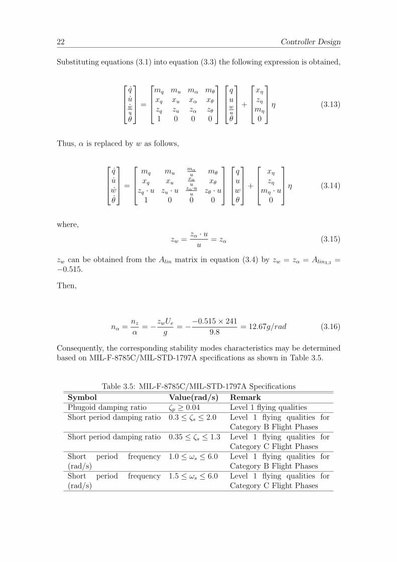
3.5 MIL-F-8785C/MIL-STD-1797A Specifications . . . . . . . . . . . . . 22
3.6 Design Requirements . . . . . . . . . . . . . . . . . . . . . . . . . . . 23
3.7 Stability Characteristics Comparison . . . . . . . . . . . . . . . . . . 29
4.1 CAP parameters(he = 7000m,VTAS = 241m/s) . . . . . . . . . . . . . 32
5.1 Stability Characteristics Comparison-Closed Loop . . . . . . . . . . . 43
5.2 CAP parameters (EP8500,180) . . . . . . . . . . . . . . . . . . . . . . . 44
A.1 Bandwidth requirements of different flight phase[Ano90] . . . . . . . . 78
C.1 Trimming and linearisation Parameters . . . . . . . . . . . . . . . . . 94

Abbreviations xiii
Abbreviations
ARI Aileron Rudder InterlinkCAD Computer Assisted DesignCAP Control Anticipation ParameterCAS Control Augmentation SystemCSAS Control and Stability Augmentation SystemDASMAT Delft University Aircraft Simulation Model and Analysis ToolFBW Fly By WireFCS Flight Control SystemFlightLab747 Flight Laboratory 747LAF Load Alleviation FunctionLPV Linear Parameter VaryingLTI Linear Time-InvariantLTV Linear Time VaryingMAC Mean Aerodynamic ChordPI Proportional-plus-Integral controlPID Proportional, Integral and Derivative controlPIO Pilot Induced OscillationRCAH Rate Command-Attitude HoldSAS Stability Augmentation SystemSISO Single-Input-Single-OutputSPPO Short-Period Pitching Oscillation

xiv Nomenclature
Nomenclature
A System matrixAlin System matrix for linearized aircraft modelB Input matrixBlin Input matrix for linearized aircraft modelC Output matrixC1 and C2 Local linear controllersClin Output matrix for linearized aircraft modelD Direct matrixDlin Direct matrix for linearized aircraft modelCAP Control Anticipation ParameterCAPopen Control Anticipation Parameter of open-loop systemCAPclosed Control Anticipation Parameter of closed-loop systeme Gain scheduling factorEP Equilibrium pointspbody Roll rate about body X-axis rad/sqbody Pitch rate about body Y-axis rad/srbody Yaw rate about body Z-axis rad/sα Angle of attack or incidence radβ Angle of sideslip radφ Roll angle radθ Pitch angle radϕ Yaw angle radγ Flight path angle radǫq Integral error variableζp Phugoid mode damping ratioζs Short period mode damping ratioζsr1 , ζsr2 The required short period mode damping ratioTlagr1 , Tlagr2 The required integral lag time constantTθ2 The incidence lag variableωp Phugoid mode natural frequency rad/sωs Short period mode natural frequency rad/sωsopen Short period natural frequency of open-loop system rad/sωsclose Short period natural frequency of closed-loop system rad/sωsr1 , ωsr2 The required Short period mode natural frequency rad/sC1, C2 the Local controllers

Nomenclature xv
F The flight envelopehe Geometric altitude mxe Horizontal position along earth X-axis mye Horizontal position along earth Y-axis mpbody Roll acceleration about body X-axis rad/s2
qbody Pitch acceleration about body Y-axis rad/s2
rbody Yaw acceleration about body Z-axis rad/s2
VTAS Time derivative of true airspeed m/s2
α Angle of attack or incidence rate rad/s
β Angle of side-slip rate rad/s
φ Roll attitude rate rad/s
θ Pitch attitude rate rad/sϕ Heading rate rad/sγ Flight path angle rate rad/s
he Geometric altitude rate m/sxe Horizontal ground speed along earth X-axis m/sye Horizontal ground speed along earth Y-axis m/sδe Elevator deflection radδstab Stabilizer deflection radTn Thrust NKn Controls fixed static stability marginK Matrix of state variable feedback gainskq Pitch rate feedback gainkα Angle of attack feedback gainkǫq Integral gainM Feed forward gain matrixqd Pitch rate demand rad/snα Normal load factor per unit angle of attack g/radUe Axial component of steady equilibrium velocity m/sV0 Steady equilibrium velocity m/sVTAS True airspeed m/snz Total normal load factor gu Axial velocity perturbation m/sv Lateral velocity m/sw Normal velocity m/sx the state vectorx the derivative of state vectoructrl input vectory output vector∆ Characteristic polynomial: Transfer function denominator

This page intentionally contains only this sentence.

Introduction 1
Chapter 1
Introduction
1.1 Background
Gain scheduling is considered as a standard method to design Linear Time-Invariant(LTI) controllers for Linear Time Varying (LTV) or nonlinear systems in control the-ory. It also has widespread and successful engineering applications, an importantexample being its implementation in the design of the flight control system of air-craft [RS99] [LL00]. The idea behind gain scheduling is that gains of controllersare scheduled with some measured parameters of the system. These measured pa-rameters of the system are usually referred to as the scheduling parameters. Inthe aerospace sector, gain scheduling technology was first used mainly on militaryapplications. By the mid 1950s, gain scheduling technology began to overcome dif-ficulties of implementing into the new generation of jet aircraft. A research subjectof gain scheduling application in civil aircraft and other areas developed graduallysince then. Recently, there has been an increasing number of research activities anda wider range of applications in the area of gain scheduling [RS99] [SG07] [RDLB03].In the light of the significant change of the aircraft aerodynamic properties through-out the wide range of operating conditions, the design of the flight control system isa typical nonlinear control problem due directly to the responsive change in aircraftdynamics with flight condition [OSBV00]. Gain scheduling is an attractive controlstrategy to deal with these nonlinearities of the aircraft flight control. In the areaof aircraft flight controller design, the main idea of gain scheduling methodology isto design a set of LTI controllers for a number of operating points and then inter-polate the parameters or gains of the flight controllers against the current value ofthe scheduling parameters varying with the flight conditions over a wide flight en-velope of an aircraft, instead of seeking a single robust LTI controller for the entireoperating range.
For the modern civil passenger aircraft, it is quite common that some form of FlightControl System (FCS) is employed to augment the dynamic characteristics of theaircraft in order to obtain desirable flying and handling qualities. A typical FCScomprises a number of actuators, motion sensors including accelerometers and rate

2 Introduction
gyros, and air data sensors. All these signals are fed back through the controller thatenacts certain flight control laws designed for a specific aircraft to control the controlsurface deflections and throttle [Coo07] [And10]. The control law is implemented byincluding one, or several control functions in the command, forward and feedbackpaths, each of which comprises multi-variable and separate loops for the aircraftinfluencing the characteristic behaviour of the augmented aircraft on the roll, pitchand yaw control axes differently.
The Control and Stability Augmentation Systems (CSAS) is an integral part of theFCS, which determines the control and stability characteristics of the augmentedaircraft. The most commonly encountered CSAS control laws are equipped with ratefeedback - improving artificial damping, C∗ - a combination of normal accelerationand pitch rate feedback to give good dynamic handling and control sensitivity, andthe longitudinal Rate Command Attitude Hold (RCAH)- that can achieve a goodpitch attitude tracking characteristic. The main purpose of the FCS that includesCSAS is to improve an aircraft’s flying and handling qualities, tracking ability andride comfort [Coo10a][And10].
The handling qualities of an aircraft are the properties that describe the effectivenessand precision by which a pilot may control the aircraft in the execution of the definedflight task or mission [Coo07] [Gib99]. For more formal analytical purposes, theseintangible properties must be described quantitatively rather than being expressedin terms of pilot opinion. The basic aerodynamic stability and control characteristicsof the airframe, and also the effects of a installed FCS, are quantified and commonlyused as indicators and measures of the handling qualities [Gib99]. Consequently, anumber of criteria have been developed for the explicit purpose of ensuring gooddynamic response characteristics to aid in the design of an airplane’s dynamic char-acteristics, such as the Control Anticipation Parameter (CAP), Neal and Smith, C∗,Gibson and Bandwidth criteria.
The main contribution of this research is to combine the gain scheduling techniquebased on the local controller design approach and handling qualities assessment. Thecontrollers are designed locally in a number of operating points and the interpolationbetween them ( i.e. scheduling) takes place through the scheduling scheme functions.The aircraft augmented with gain-scheduled controller performs satisfactorily andmeets the requirement of handling qualities. Moreover, the performance using thegain-scheduled controller is significantly improved compared to the performanceusing the fixed one.
1.2 Aim and Objectives
The aim of this project is to design a set of gain scheduling RCAH controllers foran aircraft longitudinal CSAS at different operating points to satisfy the handlingqualities requirement. This focuses on the gain scheduling technique, FCS design andhandling qualities assessment. With the aid of the handling qualities assessment,
Introduction 3
the schedule scheme will be designed. The study shall include the longitudinalRate Command-Attitude Hold (RCAH) controllers design using the state space poleplacement design procedure, handling qualities assessment over the whole flightenvelope to identify the interpolation region, and the gain scheduling against thecurrent value of the scheduling parameters (airspeed and altitude).
The objectives of this research are as follows:
• Design the longitudinal Rate Command-Attitude Hold (RCAH) controllers asthe local flight controllers based on the specific equilibrium points.
1. Trim and linearize the Boeing 747 series 100/200 aircraft model based onthe equilibrium points along with the flight envelope.
2. Employ the linear aircraft models on specific equilibrium points to aid inthe controller design and handling qualities assessment.
3. Apply the state space pole placement design procedure to design a lon-gitudinal Command and Stability Augmentation System (CSAS) withRate Command-Attitude Hold (RCAH) characteristic.
• Assess the handling qualities of the aircraft over the flight envelope.
1. Assess the handling qualities of the aircraft with local controllers to guar-antee the good dynamic response characteristics.
2. Determine the number of local controllers to cover the entire flight enve-lope with satisfactory handling qualities.
3. Identify the interpolation region by means of the handling qualities as-sessment of the local controllers in the whole flight envelope.
• Schedule the gains of the local controller in interpolation region of the flightenvelope.
1. Develop a gain scheduling scheme to ensure the controller gains aresmoothly scheduled according to the current trimmed operating condi-tions achieving satisfactory performance and handling qualities.
2. Review the influence of the flight controller with scheduled gains on thelongitudinal handling qualities of the aircraft in the interpolation region.
In this research, the mathematical model of the Boeing 747-100/200 aircraft is em-ployed for the flight controllers design and handling qualities assessment. The Boeing747-100/200 aircraft model is an aircraft mathematical nonlinear model, and it ischosen since it is
• a well-known, popular and successful aerospace control analysis platform.

4 Introduction
• easily available.The Boeing 747-100/200 aircraft model is obtained from references [EB03],[EB01] and [vdL96], which is based in Matlab/Simulink. In addition, it offersa wide range of simulation and analysis tools which make it easy to obtainlinear flight dynamics models for any flight condition.
• a typical civil transport passenger aircraft.The Boeing 747 is an intercontinental wide-body transport with four fan jetengines. The wide array of characteristics, such as leading and trailing edgeflaps, spoilers and variety of control surfaces, makes it representative of anycommercial airplanes flying today.
1.3 Summary
In summary, this thesis presents a method for the design and development of gainscheduling controllers for a passenger aircraft B747 to satisfy the handling qualitiesrequirement. With the aid of the handling qualities assessment over the whole flightenvelope, the interpolation region is identified, and furthermore, the gain schedulingscheme is determined.
This thesis is organized as follows:
Chapter 2 presents a overview of the history, as well as development and state-of-the-art in flight control system, gain scheduling methodologies and aircrafthandling qualities.
Chapter 3 describes the design process of a longitudinal Control and StabilityAugmentation (CSAS) with Rate Command Attitude Hold (RCAH) charac-teristics. This comprises the application of the Boeing 747 series 100/200 air-craft mathematical model, the process of deriving the state space equations,and the design procedure of the controller.
Chapter 4 assesses the longitudinal handling qualities of the aircraft with the lo-cal controller using existing handling qualities criteria, including the ControlAnticipation Parameter (CAP), Neal and Smith, and C∗ criteria.
Chapter 5 discusses the handling qualities over the whole flight envelope togetherwith a second controller design and identification of the interpolation region.
Chapter 6 derives the gain scheduling scheme to ensure the gains of the localcontrollers are smoothly scheduled according to the current trimmed operatingconditions with satisfactory performance and handling qualities.
Chapter 7 provides a summary of findings, concluding remarks and recommenda-tions for further work.

Literature Review 5
Chapter 2
Literature Review
This chapter presents a review of the history, the state-of-the-art of gain schedulingmethodology development as applied to the aircraft flight control system, and inparticular to satisfy handling qualities requirements. Thus the focus is on FlightControl System (FCS), gain scheduling technique and handling qualities assessment.
2.1 Flight Control System
The aircraft FCS enables the pilot to exercise control of the aircraft over all theflight, by controlling the aerodynamic control surface deflections and throttle tomodify the aircraft dynamics, and then the aircraft is endowed with manoeuvre inpitch, roll and yaw axis [MAS08]. Normally, the FCS is designed specifically for acertain aircraft, which leads to a similar functional architecture with different details[Coo10a].
For the modern civil passenger aircraft, it is quite common that some form of FCS isemployed to augment the dynamic characteristics of the aircraft in order to obtaindesirable flying and handling qualities. A typical FCS comprises a number of actua-tors, motion sensors and air data sensors. All these signals are fed back through thecontroller that enacts certain flight control laws designed for a specific aircraft tocontrol the control surface deflections and throttle [Coo07] [And10]. The control lawis implemented by including one, or several control functions in the command, for-ward and feedback paths, each of which comprises multi-variable and separate loopsfor the aircraft influencing the characteristic behaviour of the augmented aircraft onthe roll, pitch and yaw control axes differently.
2.1.1 Functional Description
The general objective of the flight control law design is to improve the flying andhandling qualities of the basic aircraft, i.e., to enhance stability and controllability.

6 Literature Review
The pilot controls’ inputs are transformed by the flight control computer into pilotcontrol objectives which are compared with the measured aircraft states. A typicalFCS is commonly comprised of measurements like air data sensors - measuring theaircraft states, such as velocity and attitude - motion sensors - measuring the aircraftattitude - as well as main functional components such as control actuators, aerody-namic control surfaces, the respective cockpit controls, connecting linkages, and thenecessary operating mechanisms to control an aircraft’s direction in flight [And10][Coo10a] [MAS08]. In general, a commercial civil passenger aircraft FCS may wellbe divided into inner loops and outer loops with the respect of the type of controlfeedback loops. Inner loops are essential to determine the stability characteristicsof an aircraft, e.g. the autostabiliser and the Stability Augmentation System (SAS)[Coo10a], while outer loops are in reference to optional functions, e.g. autopilot.
• Inner loops
1. Modern high performance aircrafts rely heavily on the inner loop of theflight control system. Principal inner loop functions, such as the autosta-bilizer and the Control and Stability Augmentation System (CSAS), playa vital role and are continuously engaged during flight to enable the air-craft to perform manoeuvres with satisfactory flying and handling qual-ities. The SAS is an integral part of the FCS to augment the flyingdynamic characteristics of the aircraft seeking for good flying qualitiesand stability, while Control Augmentation System (CAS) is additionallydesigned to modify the handling characteristics of the aircraft to improvethe performance in manoeuvre and command tracking; together, thesetwo systems are considered as CSAS [Coo07] [Coo10a] [Chu10] [And10].
2. Secondary inner loop functions are concerned with automatic control offlaps, spoilers, engines, etc. without pilot intervention. In addition, itis common that many modern aircraft employ some form of active con-trols technology such as g-limiting, α-limiting and gust load alleviation[Coo10a] [MAS08].
• Outer loopsThe outer loops are mainly concerned with autopilot functions that are selec-tively engaged during the flight. The main purpose of the autopilot is eitherto release the pilot from continuous control of an aircraft (especially for civilpassenger aircraft), or for operation in adverse conditions which are beyondthe limits of human capability (particularly for military aircraft) [Coo10a].
In this research, the FCS control law function design is concerned with the CSASof inner loop functions design. The functionality of the CSAS can be divided intothree components: the feedback path, the feedforward path and the command path.
The closed-loop control and stability characteristics of the aircraft are primarily de-signed using the feedback path. Meanwhile, the forward path can be used both todefine the closed-loop characteristics of the aircraft, and to provide control signal

Literature Review 7
response shaping. Consequently; the command path may well be used to shape thecommand by the gain to produce the actual command signal for the closed loopwithout compromising the closed-loop characteristics [OB01]. The choice of the dif-ferent control path can influence the aircraft dynamics differently, which relies onthe requirement of flying and handling qualities. The simplified typical closed loopflight control functional structure is shown on Fig. 2.1. The closed loop transferfunction thus can be obtained.
Feedforward path
F(s)-
Feedback path
H(s)
ResponseCommand
path
C(s)
Pilot
demandAircraft
dynamics
G(s)(s)
(s)
r(s)
Figure 2.1: Closed Loop Control System
2.1.2 Command and Stability Augmentation System
The main purpose of the FCS, including the CSAS, is to improve an aircraft’s flyingand handling qualities, tracking ability and ride comfort [Coo10a] [And10]. TheCSAS control law plays the key role in the entire FCS, which governs the stabilityand control characteristics of the aircraft seeking ideal flying and handling qualities.The decoupling of the longitudinal and lateral-directional motion of the aircraft givesrise to the possibility to design the longitudinal and lateral-directional CSAS controllaws separately. The longitudinal dynamics are characterized by the Short-PeriodPitching Oscillation (SPPO) mode and phugoid oscillation mode. The phugoid modeis manifested as a trimming problem, which is usually considered by the autopilot inthe FCS outer loops of the aircraft. Although it is not regarded as hazardous whenpoorly damped, it does contribute to an increased pilot workload [Coo10b]. On theother hand, the short period mode is the main factor that needs to be augmentedby the CSAS.
Before designing a CSAS, it is necessary to consider the choice of control law func-tions based on the design objectives for flying and handling qualities. The mostcommonly encountered CSAS control laws are equipped with rate feedback improv-ing artificial damping; C∗, a combination of normal acceleration and pitch ratefeedback to give good dynamic handling and control sensitivity; and the longitu-dinal Rate Command Attitude Hold (RCAH) achieving an excellent pitch attitude
8 Literature Review
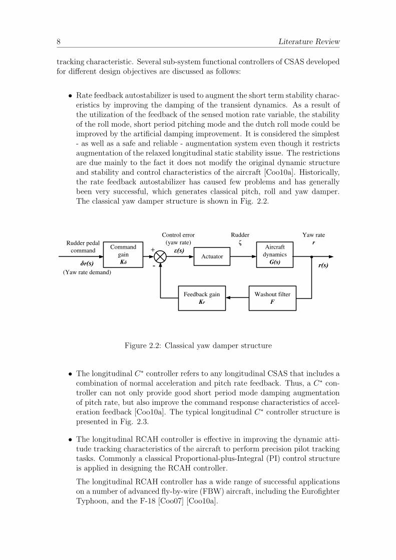
tracking characteristic. Several sub-system functional controllers of CSAS developedfor different design objectives are discussed as follows:
• Rate feedback autostabilizer is used to augment the short term stability charac-eristics by improving the damping of the transient dynamics. As a result ofthe utilization of the feedback of the sensed motion rate variable, the stabilityof the roll mode, short period pitching mode and the dutch roll mode could beimproved by the artificial damping improvement. It is considered the simplest- as well as a safe and reliable - augmentation system even though it restrictsaugmentation of the relaxed longitudinal static stability issue. The restrictionsare due mainly to the fact it does not modify the original dynamic structureand stability and control characteristics of the aircraft [Coo10a]. Historically,the rate feedback autostabilizer has caused few problems and has generallybeen very successful, which generates classical pitch, roll and yaw damper.The classical yaw damper structure is shown in Fig. 2.2.
Actuator-
Feedback gain
Kr
Yaw rate
rCommand
gain
K
Rudder pedal
commandAircraft
dynamics
G(s)r(s)
(s)
r(s)(Yaw rate demand)
Control error
(yaw rate)
Rudder
Washout filter
F
Figure 2.2: Classical yaw damper structure
• The longitudinal C∗ controller refers to any longitudinal CSAS that includes acombination of normal acceleration and pitch rate feedback. Thus, a C∗ con-troller can not only provide good short period mode damping augmentationof pitch rate, but also improve the command response characteristics of accel-eration feedback [Coo10a]. The typical longitudinal C∗ controller structure ispresented in Fig. 2.3.
• The longitudinal RCAH controller is effective in improving the dynamic atti-tude tracking characteristics of the aircraft to perform precision pilot trackingtasks. Commonly a classical Proportional-plus-Integral (PI) control structureis applied in designing the RCAH controller.
The longitudinal RCAH controller has a wide range of successful applicationson a number of advanced fly-by-wire (FBW) aircraft, including the EurofighterTyphoon, and the F-18 [Coo07] [Coo10a].

Literature Review 9
Gain-
Shaping filter
and gain
Pilot
command Aircraft
dynamics
G(s)
C* error
Elevator
Washout filter
F
C* command
Gain
Gain
C*
Actuator
Pitch rate
q
Normal
acceleration
nz
Figure 2.3: Longitudinal C∗ controller structure
For the purpose of gain scheduling techniques implementation, a generic structure ofthe longitudinal or lateral-directional flight control law, is selected. In this research,a longitudinal FCS CSAS with RCAH characteristic is employed as a local controllerto construct a global controller due mainly to the widespread application of PID andPI local control structures with scheduled gains in the FCS [LWY+08] [OSBV00].
2.2 Gain Scheduling
The idea behind gain scheduling is that the gains of controllers are scheduled withsome measured parameters of the system. These measured parameters of the systemare usually referred to as the scheduling parameters.
The recent considerable increasing interest in gain-scheduling design methodologyis not new. Gain-scheduling is one of the most popular and conventional methodsof dealing with nonlinear control systems in many engineering applications, andmuch of the classical gain-scheduling theory could date back to the early 1960s.However, in the early days, the robustness and performance could not be guaranteeddue mainly to the absence of a sound theoretical analysis regarding the issue ofthe guaranteed properties for a set of control systems with scheduled gains (linearparameter-varying plants) and nonlinear plants. The focus of attentions was on thediscussion of guaranteed performance; gain-scheduling methods did not start to beapplied to cope with nonlinear plants until the early 1990s [SA90] [RS99]. Sincethen, gain-scheduling has been established as a worthwhile design methodology fornonlinear systems control and widely and successfully applied in fields ranging fromaerospace to process control. Nowadays, gain scheduling is considered as a standardmethod to design Linear Time-Invariant (LTI) controllers for Linear Time Varying(LTV) or nonlinear systems in control theory. As such, the nonlinear system canbe approximated as a Linear Parameter Varying (LPV) system. In a conventionalgain-scheduling approach, the scheduling parameters are usually chosen from the

10 Literature Review
variables with slow variation and could capture the plant’s nonlinearities, such asaltitude, velocity, the forward velocity u, and the downward velocity w [Rad04][SA90] [RS99].
With the development of the gain-scheduling techniques, many different design no-tions can be interpreted as gain scheduling which is generally developed as a point ofview taken in the design process. The main idea of gain scheduling method is usinglinear controller design techniques to address nonlinear problems by continuouslyvarying the controller coefficients according to the current value of the schedulingparameters. Hence, the overall performance properties are determined by the localdesigns. Comprehensive overviews of gain-scheduling techniques can be derived fromthe references [LL00] and [RS99]. Recently, there has been an increasing number ofresearch activities and a wider range of applications in the area of gain scheduling,especially in the aerospace field [RS99] [SG07].
In the area of aircraft flight controller design, gain scheduling is the most commonsystematic approach to cope with the nonlinearity of the aircraft dynamics over theflight envelope. In the aerospace sector, gain scheduling technology was first usedmainly on military applications, e.g. missile guidance systems and autopilots forthe B-52. By the end of the Second World War in the mid 1950s, gain schedulingtechniques began to overcome difficulties of implementing into the new generation ofjet aircraft [RDLB03]. Since then, a research subject of gain scheduling applicationin civil aircraft developed, and gradually, it has broadened out into more widespreadengineering applications, an important example being its implementation in thedesign of the flight control system of an aircraft [RS99] [LL00] [Zhu06] [GZ94]. In thelight of the significant change of the aircraft aerodynamic properties throughout thewide range of operating conditions, the design of the flight control system is a typicalnonlinear control problem due directly to the responsive change in aircraft dynamicswith flight condition [OSBV00]. Gain scheduling is an attractive control strategyto deal with these nonlinearities of the aircraft flight control. Although it doesnot always provide controllers that guarantee closed loop stability and performance,gain scheduling design method possesses certain engineering practical advantages inaircraft flight control system design, such as simplicity, generality, low computationalcomplexity and ease of implementation [RLBC06].
In recent years, there have been several published studies of gain scheduling in air-craft flight control system design. Several synthesis algorithms have been exploitedfor systematic design of gain-scheduling controller. In order to overcome the con-straints on the maximum rates of change of the scheduling parameters, the rapidlyvarying states such as angle of attack α are adopted as the scheduling parametersinstead of the conventional scheduling parameters with slow variation [RLJD07]. Itis found that the dynamic transient response in nonlinear regions has been improved.This method for scheduling state feedback gains against rapidly varying parametersis detailed in references [RDLB03], [RLJD07] and [SB92]. Gain scheduling researchin aircraft flight control system design has been very active over the last decade. Itcould cover a wide range of subjects including the following:

Literature Review 11
• Single-input-single-output(SISO) and multivariable scheduling problem [Gar97](with respect to input/output characteristics);
• H∞ controller design [NRR93] and adaptive control [JAL08](due to the controltechniques);
• ν-gap metric [FFN03], fuzzy clustering [OBB02] [GZ94], from interpolationtechniques viewpoint;
• RCAH and coordinated turning [WSG03], from the control law functions.
The characteristic of gain scheduling methodology is to design a set of LTI controllersfor a small number of operating points and interpolate the parameters(gains) of thecontrollers in the region between operating points over a wide flight envelope of anaircraft instead of seeking a single robust LTI controller for the entire operatingrange [AEJ08].
Based on the typical gain-scheduling design procedure for nonlinear plants derivedfrom references [SA90] and [OSBV00], the design procedure of a gain scheduled flightcontrol system design for an aircraft can be stated as follows:
1. Linearize the aircraft model around a selection of equilibrium points in theflight envelope.
2. Design a linear controller for each of the linearized models as summarized insection 2.1.2. We will refer to this as the ‘local controller’.
3. Tune the coefficients (gains) of the local controller at each equilibrium point.
4. Schedule the coefficients (gains) of the local controllers resulting in a globalcontroller- this involves the implementation of a family of linear controllerssuch that the controller coefficients (gains) are scheduled according to thecurrent value of the scheduling parameters.
5. Evaluate the performance by linear analysis and non-linear simulation.
This process converges when the closed-loop aircraft dynamics are satisfactory overthe entire operating range.
Most of the efforts paid on gain-scheduling flight control system design have dealtwith the local controller design procedure as well as the identification of the operatingpoints and the design of the interpolation scheme [OSBV00] [NRR93]. Three mainaspects concerned about these two questions are as follows [OBB02]:
• The local controller design procedure
Based on the identification of the operating points, the local controllers for theaircraft longitudinal motion control can be designed for the linearized aircraft

12 Literature Review
model of the Boeing 747-100/200. In this research, the classical single-loopdesign techniques-state space pole placement is employed to develop flightcontrol laws. There has been extensive research in using advanced controldesign methods to replace the classical CSAS in the flight control law design.Such methods include H∞ multivariable design [BP02] and eigenstructure as-signment [LP98]. Although replacing the classical single-loop approach witha multi-loop enhances the performance and robustness of the controller, ithas not overcome difficulties of the development of an efficient method forscheduling of the multivariable controller for future industrialization [ARS01][OBB02]. For most of the fly-by-wire (FBW) aircraft flying today, the controllaws have been developed by using classical single-loop design techniques, suchas frequency responses, root locus and state space pole placement.
• The identification of the operating points
For implementation of classical gain scheduling, the flight envelope is subdi-vided into operating regions based on information of the aircraft dynamics asa function of flight condition at different operating points. The trial-and-errormethod is generally employed in gain-scheduling FCS design to identify theoperating points [OSBV00]. Although the operating points are selected arbi-trarily and inexplicitly by this method, the iterative approach based on thepast experience guarantee the satisfactory closed-loop aircraft dynamics overthe entire operating range in the design process.
In this study the selection of the operating points is performed using a heuris-tic method based on the handling qualities assessment. Besides the local con-trollers’ performance analysis, the aircraft handling qualities are assessed overthe flight envelope. Normally, it is not necessary to design local controllersat each operating points for the purpose of covering the whole flight envelopewith satisfactory handling qualities. Comparing to the conventional methodof dealing with controllers at each of these equilibrium points, the whole oper-ating range could be covered by a fewer number of controllers, which increasesthe efficiency of the scheduler. The advantage of applying this method to iden-tify the operating points are that the number of local linear controllers can bekept small and more importantly the global nonlinear controller complies withthe performance and handling qualities requirements.
• The design of the interpolating scheme
In this research, the conventional gain-scheduling method is considered. Theparameters with slow variation- airspeed and altitude are chosen as schedul-ing parameters to capture the nonlinear properties of aircraft flight dynamicsvarying with the flight conditions. Gains of the controller can be scheduledagainst the current value of the airspeed and altitude following the interpo-lating scheme which is an important part of the gain-scheduling FCS designprocess. The implementation of the interpolating scheme design ensures anappropriate gain-scheduled controller, and finally determines the performance

Literature Review 13
of the whole set of the controller. A number of different approaches of interpo-lating scheme design could be used, such as bumpless switching, interpolationtechniques, and linear interpolation of the parameters [ABB02] [AEJ08]. Inthis thesis, the interpolating of a family of local linearized controllers withswitching techniques of linear interpolation of the parameters is practiced toyield a global controller.
In recent years, Linear Parameter Varying (LPV) control has been established asan emerging advanced approach to be a reliable alternative to conventional gain-scheduling approach [EB01] [Chu10]. LPV is based on the principle of the H∞
multi-variable control, and the excellent performance - including command track-ing, disturbance attenuation, low sensitivity to measurement noise, and reasonablysmall control efforts - is mainly due to LPV technique theoretical property. Thewhole system is considered as a single dynamic system [Chu10]. Clearly, the con-ventional gain scheduling is a collection of dynamic systems, which means the robustperformance can not be easily guaranteed for the global controller. Although thisconventional approach can not guarantee the stability or robustness of the controllerfor each operation point of the flight envelope, this conventional approach of design-ing gain scheduled FCS for aircraft still has a wide range of applications in theengineering field due to its developed technique. Hence, this research contains acertain practical meaning as well.
2.3 Handling Qualities
The handling qualities of an aircraft are the properties that describe the effectivenessand precision by which a pilot may control the aircraft in the execution of the definedflight task or mission [Coo07] [Gib99]. For more formal analytical purposes, theseintangible properties must be described quantitatively rather than being expressedin terms of pilot opinion. Not only the basic aerodynamic stability and controlcharacteristics of the airframe, but also including the effects of an installed flightcontrol system (FCS), are quantified and commonly used as indicators and measuresof the handling qualities [Gib99]. Consequently; a number of criteria have beendeveloped for the explicit purpose of ensuring good dynamic response characteristicsto aid in the design of an aircraft’s dynamic characteristics, such as the ControlAnticipation Parameter (CAP), Neal and Smith, C∗, Gibson and Bandwidth criteria.In order to quantify the handling qualities of the B747 to aid in the identificationof the operating point and accomplish the scheduler design, the existing flying andhandling qualities criteria and specifications are reviewed.
Both civil and military handling qualities criteria or specifications exist which definethe minimum performance requirements for a given aircraft. These aircraft handlingqualities criteria and flying specifications can be specified in several ways. Militaryand civil flying specifications, such as MIL-STD-1797A and FAR-25 or CS-25. TheUS Federal Aviation Regulations (FAR-25) [Ano94] and Certification Specificationfor Large Aeroplanes (CS-25) [CS206] define a comprehensive suite of performance
14 Literature Review
and safety requirements with which any large commercial transport aircraft mustcomply if it is to be granted a certificate of airworthiness. For the handling qualitiesassessment of a civil passenger aircraft like B747, FAR-25 and CS-25 are the mostsuitable criterion to comply with. Unfortunately, there are few specifications toquantify the handling qualities in FAR25 or CS-25. For more formal analyticalpurposes, it is necessary to describe the handling qualities quantitatively. Althoughthese criteria are generally better developed for military combat aircraft, and arenot entirely applicable to the B747 aircraft, the CAP, Neal and Smith, and C∗
criteria can still be applied to assess the handling qualities of the B747 aircraft asan indicator of the degradation.
There exist many handling qualities criteria which aid the designer in the definitionof the aircraft and the specification of its dynamic characteristics [Coo07]. Theseaircraft handling qualities criteria and flying specifications are commonly definedin terms of pole-zero specifications [Ano90]. Criteria can be in terms of minimumdamping and natural frequency, or pole-position, such as the incidence lag variableTθ2 [Gib99]. Criteria can also be defined in terms of frequency response, such asminimum gain and phase margins - for example the bandwidth criterion - or timeresponse, such as the C∗ Criterion [TEM66]. Criteria can also be defined based onpilot models, such as the Neal and Smith criteria which estimates aircraft flyingqualities based on pilot model compensation requirements [TR71].
In general, flying specification requirements vary for different phases of a flight.Certain pilot tasks associated with different flight phases require more stringentrequirements in order to achieve the mission successfully. The specification require-ments are stated with respect to flight phase categories, classification of airplanesand levels of flying qualities. Those missions requiring similar flying qualities arecommonly grouped together into three flight phase categories: Categories A, B, andC [Ano90] [Ano80].
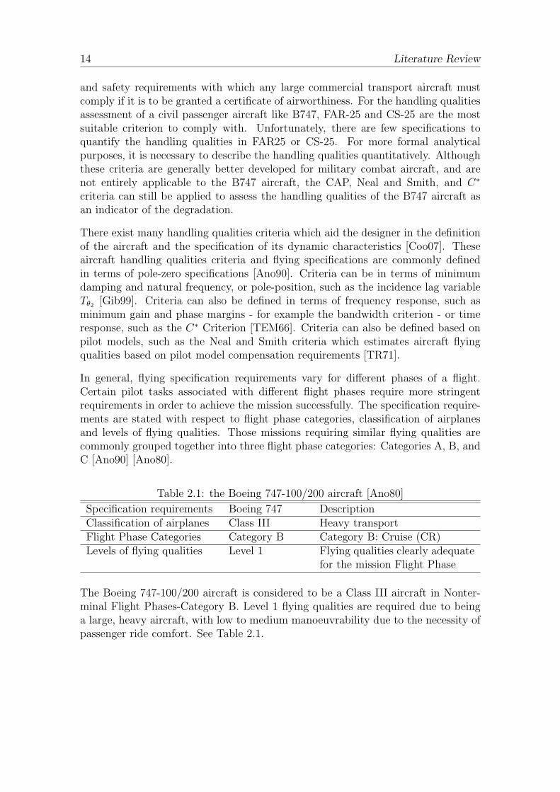
Table 2.1: the Boeing 747-100/200 aircraft [Ano80]
Specification requirements Boeing 747 DescriptionClassification of airplanes Class III Heavy transportFlight Phase Categories Category B Category B: Cruise (CR)Levels of flying qualities Level 1 Flying qualities clearly adequate
for the mission Flight Phase
The Boeing 747-100/200 aircraft is considered to be a Class III aircraft in Nonter-minal Flight Phases-Category B. Level 1 flying qualities are required due to beinga large, heavy aircraft, with low to medium manoeuvrability due to the necessity ofpassenger ride comfort. See Table 2.1.

Controller Design 15
Chapter 3
Controller Design
3.1 Aircraft Model Introduction
Before a controller of longitudinal Command and Stability Augmentation System(CSAS) can be designed, an aircraft model has to be determined. In this research,the mathematical model of the Boeing 747-100/200 aircraft is employed in aid offlight controllers design. The Boeing 747-100/200 is a wide-body commercial airlinerand cargo transport with four fan jet engines. The performance characteristics aresummarized in Table 3.1 below and the Boeing 747-200B during take-off is shownin Fig. 3.1.
Table 3.1: Boeing 747-100/200 Specifications [EB03] [B7407]
Cruising speed Mach 0.84 (893 km/h, 481 knots )(at 35,000 ft altitude)Maximum speed Mach 0.89(955 km/h, 516 kn)Maximum Range 6,100 statute miles (9,800 km) to
7,900 statute miles (12,700 km)Design ceiling 13,716 m
The Boeing 747-100/200 aircraft model employed in this research is also known asFTLAB747v6.5, which is derived from the references [EB03], [EB01] and [vdL96].FTLAB747v6.5 is developed based on Delft University Aircraft Simulation Modeland Analysis Tool (DASMAT) and the Flight Laboratory 747 (FlightLab747). BothDASMAT and Flightlab747 are originally developed by Delft University of Tech-nology. DASMAT is a general and powerful Computer Assisted Design (CAD)environment for flight dynamics and control analysis developed by C. A. A. M. vander Linden in 1996. Then, M. H. Smaili developed FlightLab747 based on DASMATin order to study the EL AL Israel Airlines crash on October 4th 1992 near Ams-terdam. Andres Marcos Esteban, who is the main developer of this model, updatedan enhanced version of the Boeing 747-100/200 aircraft model - FTLAB747v6.5 in

16 Controller Design
Figure 3.1: Boeing 747-200B [B74]
2003 which is a widespread aerospace control analysis platform still using at present.FTLAB747v6.5 is an aircraft mathematical nonlinear model, which is based in Mat-lab/Simulink and offers a wide range of simulation and analysis tools. Meanwhile, itis also an ideal test platform to test fault tolerant control, fault detection and faultdiagnostics.
In addition, FTLAB747v6.5 is well-designed with user-friendly interface. The appli-cation of this program simplified the controller design process by directly providingthe procedures of trimming and linearizing the aircraft model at the defined op-erating points. Consequently, this nonlinear model could also be used to be antest bed to evaluate the performance and handling qualities of the aircraft with thecontrollers.
For the Boeing 747-100/200 aircraft model, the flight envelope considered is shownin Table 3.2. In addition, it does not include approach and take off configurations,landing gear and the ground effects [EB03].
Table 3.2: The flight envelope of the Boeing B747 aircraft model [EB03]
Parameters Symbols Range UnitsAltitude he 5000 to 11000 mTrue airspeed VTAS 150 to 260 m/sAngle of attack α −2 to 23 deg
The aircraft is assumed to be a rigid symmetric aircraft in this model. In orderto design a FCS through conventional design methods, a linearized model - that

Controller Design 17
describe the aircraft’s flight dynamics about one specific equilibrium point - mustbe developed.
The DASMAT manual [vdL96], and the FTLAB747v6.5 manual in Chapter 6 of[EB03] provide a fuller description of FTLAB747v6.5.
The trimming and linearizing process, equations of motion, and controller designwill be introduced subsequently.
3.2 Trim and Linearization
It is considered that the moments acting on the aircraft are balanced when theaircraft is trimmed in steady flight. To trim an aircraft model is not as easy as totrim a real aircraft flying in the air. Trimming and linearizing are a mathematicallycomplex procedure for an aircraft model. For linear flight controller design, specialtools are provided in DASMAT to trim and linearize the aircraft at defined operatingpoints. Therefore, it can be realized through activating the corresponding buttonin this B747 aircraft model. This trim and linearization routine embedded in thisB747 aircraft model simplifies the process of controller design and test. However,the important thing is selection of the equilibrium points throughout the flightenvelope. See Appendix C for further information of trim and linearization tools ofFTLAB747v6.5.
3.2.1 Aircraft Model Trim
A trim point with specific flight configuration and condition is defined in this trimroutine which is tabulated in the following Table 3.3.
Table 3.3: Aircraft Configuration of Boeing 747-100/200 in Trim Routine
Aircraft Configuration ValueInitial Mass(kg) 300, 000xcg 25% MACycg 0% MACzcg 0% MACFlight Configuration Value/StatusAltitude(he) 7000 mAirspeed (VTAS) 241 m/sFour engines All workingFlight Condition Straight-and-level trim
As shown in the Table 3.3, the specific configurations of the aircraft model aredefined. The altitude (he = 7000 m) and airspeed (VTAS = 241 m/s) represent thecurrent operating condition illustrating the operating or equilibrium point where

18 Controller Design
the aircraft is trimmed. These two flight configuration observable variables are alsoselected to be the scheduling parameters in this research. The trim point (he = 7000m, VTAS = 241 m/s) is chosen as the operating point, upon which the aircraft modelis trimmed and linearized, then a flight controller is developed.
3.2.2 Aircraft Model Linearization
After flight equilibrium condition is defined in section 3.2.1, the linearization routineis performed in this section to linearize the aircraft model at the obtained operatingpoint. Similarly, the linearization routine involves several selections and settingstabulated in Table 3.4. The linearization routine is detailed in reference [EB03].
Table 3.4: Selections in Linearize RoutineType Optional Selection RemarkControl Inputs Control SurfacesMode to Linearize Symmetric Longitudinal motionObservation Groups x, xdot, uctrl All the available derivatives and(Refer to Fig. 3.2) (Refer to Fig. 3.3) states are specified for each group.Output Complexity Compact
The selection of mode type in linearize routine is important since it will directlyaffect the Alin, Blin, Clin, Dlin matrices of equations of motion for linearized aircraftmodel. More details of the longitudinal equations of motion obtained from the trimand linearization routine will be expanded in the following section. A description ofthe aircraft states and selections shown in Fig. 3.2 and Fig. 3.3 with their units aregiven in Table C.1.
3.3 Aircraft Equations of Motion
The Boeing 747-100/200 model is trimmed and linearized on the operating point(he = 7000 m, VTAS = 241 m/s) by the procedures performed in section 3.2to obtainthe body-axes longitudinal equations of motion. In considering the current flightcondition of ‘Straight-and-level trim’ defined in Table 3.3, the angle of attack issmall, that is, α ≤ 10◦, the following approximations can be made [Nel98].
α = tan−1(w
u) ∼=
w
u(3.1)
VTAS =(
u2 + v2 + w2)1/2 ∼= u (3.2)
With reference to [Coo07], the concise form of full order equations of motion aregiven by,
quα
θ
=
mq mu mα mθ
xq xu xα xθzq zu zα zθ1 0 0 0
quαθ
+
xηzηmη
0
η (3.3)

Controller Design 19
Figure 3.2: Observation outputs groups specification

20 Controller Design
Figure 3.3: Observation outputs:x, xdot, uctrl

Controller Design 21
Then, the full order equations of motion are given by,
x(t) = Alinx(t) + Blinu(t) (3.4)
where,
x(t) =[
qbody VTAS α θ]T
; (3.5)
u(t) =[
δstab δe]T
(3.6)
Alin =
−0.728 −0.00048 −1.2025 0−0.0839 −0.00547 6.00779 −9.781.0019 −0.00036 −0.515 0
1 0 0 0
(3.7)
Blin =
2.3594 4.60990 0
0.0454 0.09440 0
(3.8)
Thus the open loop characteristic polynomial can be obtained by taking the Laplacetransform of equation (3.4),
∆(s) = (s2 + 0.002564s+ 0.002525)(s2 + 1.245s+ 1.583) (3.9)
The longitudinal stability characteristics are therefore,
ζp = 0.0255, ωp = 0.0503rad/s; (3.10)
ζs = 0.495, ωs = 1.26rad/s; (3.11)
3.4 Design Requirements
Before the controller can be designed, the design requirements may be determinedbased on the American Military Specification MIL-F-8785C [Ano80] and MIL-STD-1797A [Ano90] with respect to flight phase categories, classification of airplanes andlevels of flying qualities.
According to the specification requirements stated in MIL-F-8785C and MIL-STD-1797A, the Boeing 747-100/200 aircraft is classified with Class III airplane. Theaircraft flight phase required is in Non-terminal Flight Phases-Category B (cruise)and Terminal Flight Phases-Category C (takeoff and landing), and with Level 1flying qualities. It is necessary to calculate the value of normal load factor per unitangle of attack nα following (3.12), before determining the acceptable range of shortperiod frequency ωs complied with MIL-F-8785C/MIL-STD-1797A specifications.
nα =nz
α= −
zwUe
g(3.12)
22 Controller Design
Substituting equations (3.1) into equation (3.3) the following expression is obtained,
quwu
θ
=
mq mu mα mθ
xq xu xα xθzq zu zα zθ1 0 0 0
quwu
θ
+
xηzηmη
0
η (3.13)
Thus, α is replaced by w as follows,
quw
θ
=
mq mumα
umθ
xq xuxα
uxθ
zq · u zu · uzα·uu
zθ · u1 0 0 0
quwθ
+
xηzη
mη · u0
η (3.14)
where,
zw =zα · u
u= zα (3.15)
zw can be obtained from the Alin matrix in equation (3.4) by zw = zα = Alin3,3 =−0.515.
Then,
nα =nz
α= −
zwUe
g= −
−0.515× 241
9.8= 12.67g/rad (3.16)
Consequently, the corresponding stability modes characteristics may be determinedbased on MIL-F-8785C/MIL-STD-1797A specifications as shown in Table 3.5.
Table 3.5: MIL-F-8785C/MIL-STD-1797A Specifications
Symbol Value(rad/s) RemarkPhugoid damping ratio ζp ≥ 0.04 Level 1 flying qualitiesShort period damping ratio 0.3 ≤ ζs ≤ 2.0 Level 1 flying qualities for
Category B Flight PhasesShort period damping ratio 0.35 ≤ ζs ≤ 1.3 Level 1 flying qualities for
Category C Flight PhasesShort period frequency(rad/s)
1.0 ≤ ωs ≤ 6.0 Level 1 flying qualities forCategory B Flight Phases
Short period frequency(rad/s)
1.5 ≤ ωs ≤ 6.0 Level 1 flying qualities forCategory C Flight Phases
Controller Design 23
3.5 Controller Design
The first step in the CSAS design procedure is to establish a stability augmentationdesign objective. The MIL-F-8785C/MIL-STD-1797A specifications in Table 3.5are compared to the longitudinal stability characteristics of the basic aircraft modelobtained in cruise configuration, presented in Table 3.6. Clearly, the phugoid damp-
Table 3.6: Design Requirements
Symbol MIL-F-8785C/ B747 aircraft modelMIL-STD-1797A
Phugoid damping ratio ζp ≥ 0.04 ζp = 0.0255Short period damping ratio 0.35 ≤ ζs ≤ 1.3 ζs = 0.495Short period frequency (rad/s) 1.0 ≤ ωs ≤ 6.0 ωs = 1.26
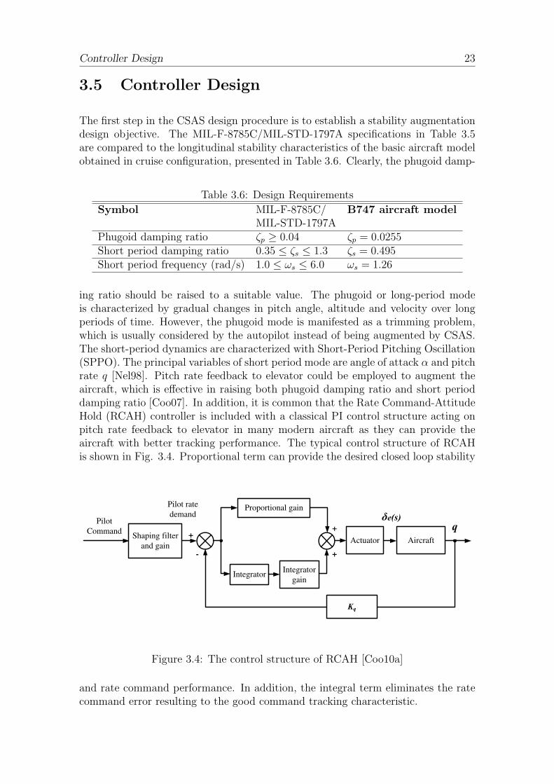
ing ratio should be raised to a suitable value. The phugoid or long-period modeis characterized by gradual changes in pitch angle, altitude and velocity over longperiods of time. However, the phugoid mode is manifested as a trimming problem,which is usually considered by the autopilot instead of being augmented by CSAS.The short-period dynamics are characterized with Short-Period Pitching Oscillation(SPPO). The principal variables of short period mode are angle of attack α and pitchrate q [Nel98]. Pitch rate feedback to elevator could be employed to augment theaircraft, which is effective in raising both phugoid damping ratio and short perioddamping ratio [Coo07]. In addition, it is common that the Rate Command-AttitudeHold (RCAH) controller is included with a classical PI control structure acting onpitch rate feedback to elevator in many modern aircraft as they can provide theaircraft with better tracking performance. The typical control structure of RCAHis shown in Fig. 3.4. Proportional term can provide the desired closed loop stability
Proportional gain
+
-
Kq
q
-
Integrator
Pilot
CommandShaping filter
and gain
Pilot rate
demand
Integrator
gain
Actuator Aircraft
+
+
e(s)
Figure 3.4: The control structure of RCAH [Coo10a]
and rate command performance. In addition, the integral term eliminates the ratecommand error resulting to the good command tracking characteristic.

24 Controller Design
3.5.1 Augmenting the Reduced Order Mode State Equation
The short period characteristics are more important in flying and handling qualitiesconsiderations. The reduced order state equation of aircraft short period mode canbe obtained by decoupling the full order of equations of longitudinal motion (3.4),which is given by,
[
qα
]
=
[
−0.728 −1.20251.0019 −0.515
] [
qα
]
+
[
4.60990.0944
]
δe (3.17)
The longitudinal equations of motion are now simplified to describe short termdynamics only. The reduced order transfer functions can be given as follows, bytaking the Laplace transform of equation (3.17).
q(s)
δe(s)=
4.6099(s+ 0.4905)
(s2 + 1.243s+ 1.58)(3.18)
α(s)
δe(s)=
0.094396(s+ 49.66)
(s2 + 1.243s+ 1.58)(3.19)
The longitudinal stability characteristics of short period mode are therefore,
ζs = 0.495, ωs = 1.26rad/s; (3.20)
The additional integrator state variable denoted ǫq(s) is employed to augment thestate equation, which is shown in Fig. 3.5. qd is pitch rate demand. The stateequation can by written as
ǫq(t) = q(t)− qd(t) (3.21)
The open loop augmented state equation can be obtained by adding the integral
Pilot
demand
G(s)
qd(s)
q(s)
1/s
e(s)
(s)
q(s)
Figure 3.5: Additional Integrator
state equation (3.21) to the reduced order state equation (3.17) as follows,
qαǫq
=
−0.728 −1.2025 01.0019 −0.515 0
1 0 0
qαǫq
+
4.60990.0944
0
δe +
00−1
qd (3.22)

Controller Design 25
The general pattern of open loop state equation and feedback control law are asfollows,
x = Ax+ Bu+Nv (3.23)
u = −Kx+Mv (3.24)
where, K is the matrix of state variable feedback gains and M is the matrix of feedforward variable gains. The closed loop system state equation can be obtained inthe general form by solving the equations (3.23) as,
x = [A− BK]x+ [BM +N ]v (3.25)
The suitable selection of gain matrices K and M is the main task in designing theRCAH controller. As can be observed from (3.25), the stability of the controlleris governed by suitable selection of gain matrices K and M , which determine thesystem response transients of the controller. In other words, the suitable choice ofgain matrices K and M is associated with the location of poles and zeros of thesystem in the s-plane. The design process is presented in the following sections.
3.5.2 Designing the Gain Matrix K
The pole placement approach is employed in designing the gain matrix K, where,
K =[
kq kα kǫq]
(3.26)
First of the most, to determine the location of the desirable closed-loop poles of thesystem base on the relevant flying qualities specification for the B747, where theAmerican Military Specification MIL-F-8785C/MIL-STD-1797A is employed. Ascan be obtained from (3.22), the system is the third order, which results in thethree poles in the closed loop characteristic polynomial. The three poles includea complex pair describing the short period mode characteristics and a real rootrepresenting the integral lag due to the additional integral term. The initial designdecisions made through designing comprises the new stability characteristics of theaugmented aircraft, which are ζsr1 , ωsr1 and Tlagr1 .
• The short period mode damping ratio of the unaugmented aircraft is ζs = 0.495as shown in Table 3.6. Although this value meets MIL-F-8785C/MIL-STD-1797A specification, it is decided to modify this value into ζsr1 = 0.75 for asmaller overshoot. It is always a good initial choice as the quickest settlingtime after a disturbance combined with the smallest overshoot.
• The short period mode natural frequency of the unaugmented aircraft is ωsr1 =1.26 rad/s as shown in Table 3.6. For the purpose of meeting the requirementsof MIL-F-8785C/MIL-STD-1797A specification as well as obtaining the de-sirable response speed and settling time, the value of natural frequency ωs israised up from original 1.26 rad/s into ωsr1 = 1.9 rad/s.

26 Controller Design
• Not only a good knowledge of the theory of the PI controller, but also more de-sign experiences are needed to choose the integral lag pole value Tlagr1 [Coo10a].The integral lag time constant Tlagr1 = 1.8 is chosen, considering it should benearer to the short period mode frequency ωsr1 = 1.9.
The controller design procedure applied in this thesis and the decisions made above,are mainly based on the reference of ‘Flight Qualities and Flight Control LectureNotes’, for further information refer to [Coo10a].
The required closed loop characteristic polynomial is thus given by,
∆(s) = (s+ 1.8)(s2 + 2.85s+ 3.61) (3.27)
The feedback gain matrix K can be calculated as follows using pole placementmethod ‘place.m’ routine in MATLAB.
K =[
kq kα kǫq]
=[
0.7331 −1.672 2.8741]
(3.28)
where, kq = 0.7331 rad/rad/s, kα = −1.672 rad/rad/s, kǫq = 2.8741 rad/rad/s.Thus the augmented state space can be written by,
qαǫq
=
−4.2927 6.5048 −13.24900.9289 −0.3573 −0.2713
1 0 0
qαǫq
+
4.60990.0944
0
δe +
00−1
qd (3.29)
3.5.3 Designing the Feedforward Gain Matrix M
Commonly, a feedforward controller is used to improve the transient performance ofthe closed-loop system. The feedforward gain matrix M is comprised with the onlyparameter-m due to the only input signal.
qαǫq
=
−4.2927 6.5048 −13.24900.9289 −0.3573 −0.2713
1 0 0
qαǫq
+
4.6099m0.0944m
−1
qd (3.30)
where m can be calculated according to the following equations.
m =kǫqTlag
=2.8741
1.8= 1.597 (3.31)
3.5.4 Implementing the Controller Design
The control law (3.24) can now be given by,
δe = −[
0.7331 −1.672 2.8741]
qαǫq
+ 1.597 · qd (3.32)

Controller Design 27
Proportional gain
kq=0.864
+
-
k =-1.672
q(s)
-
Integrator
1/s
Pilot
CommandShaping filter
and gainPilot rate
demand
qd(s)
Integrator
gain
k q=2.8741
+
+ e(s)
(s)
+
+
-
Feed-forward Gain
m-kq=0.3626
q(s)
Figure 3.6: RCAH system structure
The corresponding augmented system structure is shown in Fig. 3.6. From (3.28)and (3.31), both the feedback gain matrix K and the feedforward gain matrix Mare obtained. In consequence, the closed loop state equation (3.25) is given by,
qαǫq
=
−4.2927 6.5048 −13.24900.9289 −0.3573 −0.2713
1 0 0
qαǫq
+
7.36060.1507−1
qd (3.33)
The closed loop transfer functions are obtained as follows.
q(s)
qd(s)=
7.3606(s+ 0.4905)(s+ 1.8)
(s+ 1.8)(s2 + 2.85s+ 3.61)=
7.3606(s+ 0.4905)
(s2 + 2.85s+ 3.61)(3.34)
α(s)
qd(s)=
0.15072(s+ 49.66)(s+ 1.8)
(s+ 1.8)(s2 + 2.85s+ 3.61)=
0.15072(s+ 49.66)
(s2 + 2.85s+ 3.61)(3.35)
ǫq(s)
qd(s)=
−(s+ 1.8)(s− 4.511)
(s+ 1.8)(s2 + 2.85s+ 3.61)=
−(s− 4.511)
(s2 + 2.85s+ 3.61)(3.36)
The controller is designed based on the reduced order equations of longitudinalmotion. As can be observed from equations (3.34), (3.35), and (3.36), the designobjective of minimizing the effect of the time lag introduced by the integral term, isachieved by near exact integral pole-zero cancellation. The response to a unit stepcommand qd is shown in Fig. 3.7. It is clear that a second-order-like response isachieved to pilot controls due to the cancellation of integral pole-zero.
3.5.5 Checking the Design with the Full Order Aircraft Model
In this section, the controller would applied into the full order equations of longitu-dinal motion to ensure that the integral lag time constant is sufficiently fast withoutcausing intrusive issue. The unaugmented state space of full order equations oflongitudinal motion obtained from (3.4) is augmented by adding the integral state

28 Controller Design
0 1 2 3 4 5 6 7 8 9 100
1
2
3
Time(sec)
q(de
g/s)
0 1 2 3 4 5 6 7 8 9 100
1
2
3
Time(sec)
α(de
g)
0 1 2 3 4 5 6 7 8 9 10−0.5
0
0.5
1
1.5
Time(sec)
ε q(d
eg/s
)
Figure 3.7: Reduced order augmented aircraft response to the unit step demand
equation (3.21) as follows,
q
VTAS
α
θǫq
=
−0.728 −0.00048 −1.2025 0 0−0.0839 −0.00547 6.00779 −9.78 01.0019 −0.00036 −0.515 0 0
1 0 0 0 01 0 0 0 0
qVTAS
αθǫq
+
4.60990
0.094400
δe+
0000−1
qd
(3.37)The control law, equation (3.24) is amended as follows.
δe = −[
kq kVTASkα kθ kǫq
]
qVTAS
αθǫq
+mqd (3.38)
= −[
0.7331 0 −1.672 0 2.8741]
qVTAS
αθǫq
+ 1.597 · qd (3.39)

Controller Design 29
The full order closed loop state equation can be obtained as follows by substitutingequation (3.39) into equation (3.37).
q
VTAS
α
θǫq
=
−4.2927 −0.0005 6.5048 0 −13.2490−0.0839 −0.0055 6.0078 −9.7850 00.9289 −0.0004 −0.3573 0 −0.2713
1 0 0 0 01 0 0 0 0
qVTAS
αθǫq
+
7.36060
0.15070−1
qd
(3.40)The full order augmented aircraft transfer functions can be given as follows, by tak-ing the Laplace transform of equation (3.40). Comparing stability characteristics ofthe augmented full order equations of motion to the reduced order one, the varia-tions are tabulated in Table 3.7.
q(s)
qd(s)=
7.3606(s+ 0.00989)(s+ 0.486)(s+ 1.8)
(s+ 1.801)(s+ 0.005983)(s2 + 2.849s+ 3.61)(3.41)
VTAS(s)
qd(s)=
0.28771(s− 96.37)(s+ 1.8)(s+ 1.274)
s(s+ 1.801)(s+ 0.005983)(s2 + 2.849s+ 3.61)(3.42)
α(s)
qd(s)=
0.15072(s+ 49.66)(s+ 1.8)(s2 + 0.005432s+ 0.003401)
s(s+ 1.801)(s+ 0.005983)(s2 + 2.849s+ 3.61)(3.43)
θ(s)
qd(s)=
7.3606(s+ 1.8)(s+ 0.486)(s+ 0.00989)
s(s+ 1.801)(s+ 0.005983)(s2 + 2.849s+ 3.61)(3.44)
ǫq(s)
qd(s)=
−(s− 4.511)(s+ 1.8)(s2 + 0.005496s+ 0.003053)
s(s+ 1.801)(s+ 0.005983)(s2 + 2.849s+ 3.61)(3.45)
As can be observed from the Table 3.7, it is clear that the characteristics and
Table 3.7: Stability Characteristics Comparison
Mode Basic aircraft Reduced order aircraft Full order aircraftShort period ζs = 0.495, ζs = 0.75, ζs = 0.7497,
ωs = 1.26 rad/s ωs = 1.9 rad/s ωs = 1.9 rad/sPhugoid ζp = 0.0255, N/A T1 =
10= ∞s,
ωp = 0.0503 rad/s T2 =1
0.006163= 172.41 s
Integral lag N/A Tlag =11.8
= 0.56 s Tlag = 0.56 s
the integral lag time of full order aircraft are not significantly changed comparingwith the short period mode. However, phugoid mode is on the other hand. Thebig changes occurred to the phugoid mode result from the integral feedback. Theintegral term of pitch rate q is equal to pitch attitude θ feedback, which is animportant variable in phugoid mode, gives rise to the change in phugoid dynamics.The phugoid mode is then represented by a neutrally stable pole T1 and a stablelong time constant pole T2 instead of the second order oscillatory which would notbe obvious for pilot to handle the aircraft. Full order augmented aircraft responseto the unit step demand qd is shown in Fig. 3.8. In the first diagram, pitch rateq responds and settles to a steady value within 4 seconds after the short period

30 Controller Design
transient has damped out. The characteristics are related with the integral lag timeconstant Tlagr1 to give rise to a faster response. Since the demand qd is a unit stepfor pitch rate of 1 deg/s, the pitch attitude θ ramps up at 1 deg/s which leaves theaircraft climbing.
0 1 2 3 4 5 6 7 8 9 10 11 12 13 14 15
−1
1
3
q(de
g/s)
0 1 2 3 4 5 6 7 8 9 10 11 12 13 14 15−1000
−500
0
500
VT
AS(m
/s)
0 1 2 3 4 5 6 7 8 9 10 11 12 13 14 150
1
2
3
α(de
g)
0 1 2 3 4 5 6 7 8 9 10 11 12 13 14 150
5
10
θ(de
g)
0 1 2 3 4 5 6 7 8 9 10 11 12 13 14 15−1
0
1
2
Time(s)
ε q(deg
)
Figure 3.8: Full order augmented aircraft response to the unit step demand

Handling Qualities Assessment 31
Chapter 4
Handling Qualities Assessment
In this chapter, the handling qualities of the aircraft with configuration he = 7000mand VTAS = 241m/s are assessed. Both basic aircraft and the aircraft augmentedwith a longitudinal Rate Command-Attitude Hold (RCAH) controller are discussedrespectively. Many existing criteria and specifications are applied to assess thelongitudinal handling qualities of aircraft. The following criteria are used in thischapter to see if they could give consistent results.
• The Control Anticipation Parameter(CAP) criterion.
• The Neal and Smith criterion.
• The C* criterion
4.1 The CAP Assessment
CAP is defined in terms of short period natural frequency ωs and the normal loadfactor per unit angle of attack nα, which is given by
CAP =q(0)
Nz(∞)= −
gω2s
zwUe
=ω2s
nα
(4.1)
where nα values are given by equation (3.12), and the corresponding ωs values areobtained from Table 3.7 for basic aircraft and augmented reduced order aircraftrespectively.
The value of the parameters, such as the short period frequency ωs, and the normalload factor per unit angle of attack nα, are given in Table 3.7 with respect tothe basic and augmented reduced order aircraft models. Subsequently, the CAPparameters are calculated based on the parameters obtained, and presented in Table4.1. The results of comparing the CAP parameters of the basic and augmented

32 Handling Qualities Assessment
Table 4.1: CAP parameters(he = 7000m,VTAS = 241m/s)Parameters Open-loop Closed-loop Unitsnα 12.66 12.66 g/radω ωsopen=1.26 ωsclose=1.9 rad/sCAP CAPopen=0.125 CAPclose=0.285 -
100
101
102
10−1
100
101
102
nα (/rad)
Sho
rt p
erio
d na
tura
l fre
quen
cy
ωs(r
ad/s
ec)
Category B Flight Phase
3.6
Level 1
Level 1
0.085
nα=12.66/rad
0.038
Level 2
10.0
ω2s/nα
(CAP)
Level 2 & 3
VTAS
=241m/s, he=7000m
Open loop
Closed loop
ωs=1.26rad/s
ωs=1.9rad/s
Figure 4.1: CAP assessment for Short period mode characteristics [Ano80]

Handling Qualities Assessment 33
aircraft are plotted against the Category B requirement defined according to MIL-F-8785C/MIL-STD-1797A specification in Fig. 4.1.
As can be observed from Fig. 4.1, both CAP parameters are located in the Level 1region for a category B (Cruise) flight phase. However, the augmented B747 aircraftshows less marginal Level 1 flying qualities than the basic aircraft does. From Fig.4.1, the short period natural frequency of basic aircraft ωsopen = 1.26 rad/s is shownto be located near the bottom boundary of Level 1, while the higher short periodnatural frequency of augmented aircraft ωsclose = 1.9 rad/s is more desirable. Withthis higher value, the aircraft handling qualities are now well inside the CAP Level1 handling qualities requirements due to the aircraft being augmented by increasingthe short period frequency.
4.2 The Neal and Smith Criterion Assessment
The Neal and Smith criterion has emerged as a critical measure of pilot handlingopinion, in particular for the pitch tracking task. The Neal and Smith criterionassumes that the pilot adjusts the phase and gain characteristics to minimize thelow-frequency droop and closed-loop resonance of the aircraft [TR71]. The crite-ria are developed based on the hypothesis that if satisfactory closed-loop dynamicperformance can be achieved by the pilot model described by the assumed character-istics, then the satisfactory closed-loop dynamic performance will also be achievablefor the human pilot with acceptable workload [Ano90].
The handling qualities of the basic aircraft as well as the augmented aircraft areassessed, and results compared by means of the Neal and Smith criterion in thissection. Applying the handling qualities assessment method of the Neal and Smithcriterion presented in Appendix A, the assessment results both with and withoutthe controller engaged are shown in Fig. 4.2.
Fig. 4.2 indicates that for short period mode, an increased natural frequency from1.26 rad/s to 1.9 rad/s effectively reduced the pilot compensation. Meanwhile,the improvement of damping ratio from 0.495 to 0.75 decreases the closed loopresonance peak substantially. Both of these endow the aircraft with the Level 1handling qualities according to the Neal and Smith Criterion specification.

34 Handling Qualities Assessment
−40 −20 0 20 40 60 80−2
0
2
4
6
8
10
12
14
16
Pilot Phase Compensation [deg]
Res
onan
ce [d
B]
Level 2
Level 3
Tendency to oscillate
Good responsive airplane
Open loop
Level 1
Strong PIO tendency
Close loop
Figure 4.2: Neal and Smith criterion assessment comparison [Coo10a]
4.3 The C∗ Criterion Assessment
Boeing Airplane Company developed C∗ as a handling qualities criterion during theearly 1960s which was later developed into the basis for flight control law design[Coo10a][Ste01]. C∗ is a combination of pitch rate q and normal acceleration asshown in equation (4.2). Pitch rate dominates as a measure of aircraft handlingqualities at airspeeds less than the cross over velocity Vco, while normal accelerationnz dominates at airspeeds greater than Vco. C
∗ is a dimensionless response parametercomprising nz and q as sensed at the pilot’s station in the aircraft and is defined by,
C∗ = nz +Kq (4.2)
The transfer function usually used in practice is given by [Coo10a],
C∗(s)
η(s)=
1
g∆(s)
(
(VTAS + Vco + ls)N qη (s)− sNw
η (s))
(4.3)
where,
• VTAS = 241m/s.
• Vco = 122m/s; the airspeed, at which the q and nz contributions to C∗ transfer
function is equal during steady manoeuvres, is referred to as the cross overvelocity Vco. The value of the cross over velocity Vco based on experimentalwork was suggested as 122m/s in this instance. At speeds above 122m/s, thenz contribution dominates, and at speeds below [Coo10a]the Kq contributiondominates.

Handling Qualities Assessment 35
• l = 26.2m; the distance from the pilot station to the 25% MAC as found inNASA-CR-1756 [RH71].
• The following equations obtained from (3.34) and (3.36), are the transfer func-tions of pitch rate and angle of attack response to elevator at configurationVTAS = 241m/s and he = 7000m.
∆(s) = s2 + 2.85s+ 3.61 (4.4)
N qη (s) = 7.3606(s+ 0.4905) (4.5)
Nwη (s) = VTAS ·Nα
η (s) = 241× 0.15072(s+ 49.66) = 36.3235(s+ 49.66)
(4.6)
where,
– ∆(s) is the closed-loop characteristic polynomial of the aircraft shortperiod mode.
– N qη (s) is the numerator of the reduced order closed-loop aircraft transfer
function of q.
– Nwη (s) is the numerator of the reduced order closed-loop aircraft transfer
function of w.
Substituting the data above into equation (4.3) gives,
C∗(s)
η(s)=
(15.82s2 + 98.16s+ 133.7)
(s2 + 2.85s+ 3.61)(4.7)
The normalized C∗ transfer function is given by,
lims→0
(
C∗(s)
η(s)
)
= 37.04 (4.8)
(
C∗(s)
η(s)
)
norm
=(0.4271s2 + 2.65s+ 3.61)
(s2 + 2.85s+ 3.61)(4.9)
Apply the initial value theorem,
lims→∞
(
C∗(s)
η(s)
)
= 0.4271 (4.10)
The normalized C∗ transfer function is plotted in time domain with step responseand Bode plot respectively in Fig. 4.3. The envelope plotted in Fig. 4.3 representsacceptable limits of C∗ defined for Flight Phase Category C. Fig. 4.3 indicates theaugmented aircraft possesses acceptable handling qualities in takeoff and landingflight phase. The handling qualities assessment is limited to the flight phase cate-gory B due to the approach and take off configurations not being included in theaircraft model. However, it is considered that the C∗ assessment still possesses acertain meaning to predict the handling qualities of the augmented aircraft in FlightPhase Category B, which can also be expanded into Flight Phase Category C. Inother words, the C∗ response of the augmented aircraft is evaluated in a envelopeof a more complex and critical configuration (Flight Phase Category C), in orderto systematically analyze and obtain an overview of the handling qualities of theaugmented aircraft.

36 Handling Qualities Assessment
0 0.5 1 1.5 2 2.5 3 3.5 40
0.5
1
1.5
2
2.5
Step Response
Time (sec)
Am
plitu
de
Boundary of Flight Phase Category C
Boundary of Flight Phase Categroy C
C*
(a) C∗ step response
10−1
100
101
102
−25
−20
−15
−10
−5
0
5
10
15
Mag
nitu
de (
dB)
Bode Diagram
Frequency (rad/sec)
C*
Flight Phase Category C
Flight Phase Category C
(b) C∗ frequency response
Figure 4.3: The C∗ criterion applied to B747 [Coo10a]

Assessment over the Whole Flight Envelope 37
Chapter 5
Assessment over the Whole FlightEnvelope
This chapter presents the handling qualities assessment in the range of the entireflight envelope, together with a second controller design and identification of inter-polation region.
5.1 Introduction
In order to guarantee desirable handling qualities, a set of equilibrium points is de-fined that covers the flight envelope. The handling qualities are assessed at eachpoint in this chapter. For the flight conditions that handling qualities are not satis-fied, a second controller is designed so that the handling qualities criteria are satisfiedover the whole region therefor.
Before the different controllers and equilibrium points that are involved in the as-sessment are considered, it is necessary to clarify some of the terminology used inthis chapter.
• The controller designed in Section 3.5 is based on the aircraft operating at aparticular point in the flight envelope, namely he = 7000 m and VTAS = 241m/s. In the remainder of this thesis, this controller is referred to as C1 andthe corresponding operating point as EP(7000,241).
• The second local controller designed on operating point he = 8500m andVTAS = 180m/s is referred to as C2 and the operating point as EP(8500,180).The principle of the choice of EP(8500,180) for C2 is that the whole operat-ing range could be covered by a fewer number of controllers, which increasesthe efficiency of the scheduler. A heuristic method is applied to identify theoperating points based on the handling qualities assessment.
• The entire flight envelope is referred to as F .

38 Assessment over the Whole Flight Envelope
Clearly, the performance of the controller C1 will deteriorate as the aircraft movesaway from EP(7000,241) unless some controller scheduling is implemented. The regionF1 - where the aircraft with controller C1 generally has satisfactory handling qualities- need to be identified by the Neal and Smith criterion. So that the desired globalperformance and handling qualities in F can be guaranteed, a second controller C2
is designed with adequate handling qualities based on EP(8500,180). Similarly, theregion F2 - where the aircraft with controller C2 generally has satisfactory handlingqualities - is identified as well. Consequently, in the next chapter, gains of C1 andC2 are smoothly scheduled with altitude and airspeed showing the flight conditiontransferring from F1 to F2.
The objectives in this chapter are to
1. assess the handling qualities of the aircraft with controller C1 over a set ofoperating points in F , that covers the whole of the flight envelope. The regionF1 is then determined.
2. design a second controller based on an appropriate operating point that hasadequate handling qualities, here after referred to as C2.
3. assess the handling qualities of the aircraft with controller C2 over F , whichresults in the region F2.
4. divide F into three subsets- FC1 , FC2 and FC12 . Based on the determinationof the regions of F1 and F2; FC1 , FC2 and FC12 are identified, such thatF = FC1 ∪ FC2 ∪ FC12 and so that the aircraft with controller C1 generallyhas superior handling qualities over FC1 and the aircraft with controller C2
generally has superior handling qualities over FC2 . For FC12 , the aircraft withscheduled gains generally has superior handling qualities. Gain schedulingstrategy is designed in the next chapter.
5.2 Handling Qualities Assessment of Aircraft with
C1 in F
As pointed out earlier, the handling qualities of the aircraft with controller C1 areassessed over a set of operating points in F in this section.
5.2.1 Aircraft Models and the B747 flight envelope F
A set of the operating points along with the B747 flight envelope need to be defined,correspondingly, a set of local linear aircraft models and F need to be developedbefore the controller C1 can be assessed.

Assessment over the Whole Flight Envelope 39
Following the trim and linearization routine described in section 3.2, a set of locallinear aircraft models can be obtained from the equations of motion based on thespecific chosen equilibrium point.
Considering the aircraft model flight condition: ‘Straight-and-level trim’ chosen insection 3.2 and the flight envelope shown in Table 3.2, the flight envelope F is thendetermined by combining these two aspects with the B747 operating flight envelopederived from NASA-CR-2144 [HJ72]. Consequently, as shown in Fig. 5.1, the flightenvelope F is obtained and a set of operating points is defined, based on which acorresponding set of trimmed and linearized aircraft models is developed.
120 140 160 180 200 220 240 260 280 3003000
4000
5000
6000
7000
8000
9000
10000
11000
12000
13000
14000
Airspeed (m/s)
Alti
tude
(m
)
Flight Envelope of B747
F
Figure 5.1: Trim and linearization equilibrium points in F [HJ72]
As shown in the Fig. 5.1, the trimmed and linearized aircraft models covered theentire flight envelope F with interval of airspeed of 10m/s and altitude of 500m.The airspeed range is from 142m/s to 260m/s, and the altitude range is from 5000mto 12190m. The sea level configuration is not considered.
5.2.2 Identification of F1
The handling qualities assessment of the aircraft augmented by C1 in F is conductedin this section. Furthermore, F1, the region where the aircraft with controller C1
generally has satisfactory handling qualities, is determined. In order to identify F1,controller C1 is implemented to augment the set of aircraft models in F obtained inthe previous section. Handling qualities are then assessed systematically.

40 Assessment over the Whole Flight Envelope
• Implementation of controller C1
The control law derived from equation 3.32 is applied to augment the set ofaircraft models in F .
• Systematical handling qualities assessmentNeal and Smith criterion are utilized to assess the handling qualities of theaircraft augmented by C1 in F , and these are plotted in Fig. 5.2.
Fig. 5.2 shows the variation in Neal and Smith parameters with change in altitudeand airspeed, which is divided into two cases to be analyzed.
Case 1: At constant airspeed with increase in altitude For a constant air-speed, the augmented aircraft is more sluggish and tends to oscillate withstrong Pilot Induced Oscillation (PIO) tendency in the case of higher altitude.While, for the basic aircraft, a strong PIO tendency tends to happen at highairspeeds and a low altitude (like EP(260,5000)), which gets the opposite resultsto the augmented aircraft in the same situation . Consequently, for the aug-mented aircraft, there is a general trend towards an increasing requirementof pilot compensation and resonance peak amplitude with increasing altitude,which results in a prediction of considerably degraded handling qualities.
Case 2: At constant altitude with increase in airspeed For the aircraft aug-mented by C1, the resonance peak drops indicating larger damping in pitch os-cillations at constant altitude with increasing airspeed from 150m/s to 260m/s,and the system is less sluggish. On the other hand the basic aircraft tends to bemore sluggish and has less damping in the same situation which causes largerpilot compensation or more damping required from the FCS. Consequently, foraugmented aircraft, there is a general trend towards a decreasing requirementof pilot compensation and resonance peak amplitude with increasing airspeed,which results in a prediction of desirable handling qualities.
In summary, handling qualities of the basic aircraft and augmented aircraft arequite different with variation in altitude and airspeed. The handling qualities of thebasic aircraft represent the natural response of aircraft changing with airspeed andaltitude, while handling qualities of augmented aircraft are more dependent on theequilibrium points which the flight controller is designed for. Overall, as predictedby the Neal and Smith criterion, handling qualities are improved enormously byflight controller C1, especially for the equilibrium points near EP(7000,241) in F .Consequently, F1 is now determined, which is shown in Fig. 5.3. Note that F1 isdetermined approximately - it is a ‘piece-wise approximation’.
As can be indicated in Fig. 5.3, F1 is located in the bottom right corner of F , andthe low speed and high altitude area in F is not covered. In order for F to becovered efficiently, EP(8500,180) is chosen as the the second equilibrium point, basedon which the second controller C2 is designed.

Assessm
entover
theW
hole
Flig
htEnvelo
pe
41
−40 −20 0 20 40 60 80−2
0
2
4
6
8
10
12
14
16
Pilot phase compensation at ω=1.5 rad/s
Clo
sed
loop
res
onan
ce(d
B)
Level 1Level 2Zero phase compensationAugmented AircraftBasic Aircraft
Level 2
Level 1
Tendency to oscillate
Good responsive airplane
Phase Lag Phase Lead
Level 3
Sluggish responseStrong PIO tendency
Case 2
Case 1
(As=150,Alt=12000)
(As=260,Alt=5000)
Figu
re5.2:
Neal
andSmith
param
etersofC
1with
chan
gein
altitudean
dairsp
eed

42Assessm
entover
theW
hole
Flig
htEnvelo
pe
120 140 160 180 200 220 240 260 280 3003000
4000
5000
6000
7000
8000
9000
10000
11000
12000
13000
14000
Airspeed (m/s)
Alti
tude
(m
)
Flight Envelope of B747
EP(7000,241)
C1
F
F1
Figu
re5.3:
Identifi
cationof
F1

Assessment over the Whole Flight Envelope 43
5.3 Controller(C2) Design for the Second Equilib-
rium Point EP(8500,180)
In the previous section, equilibrium point EP(8500,180) has been chosen as the secondequilibrium point. In this section, the controller C2 would be designed based onEP(8500,180) using the similar design procedure as the controller C1 in section 3.5,which is presented in Appendix B. Controller C1 in chapter 3.5 and C2 in thischapter are designed based on the equilibrium points EP(7000,241) and EP(8500,180)
respectively. The main stability characteristics are tabulated in Table 5.1.
Table 5.1: Stability Characteristics Comparison-Closed Loop
Controller C1 C2
Equilibrium point EP(7000,241) EP(8500,180)
Short period ζs = 0.75 ζs2 = 0.8ωs = 1.9 rad/s ωs2 = 1.7 rad/s
Phugoid T1 =10= ∞s T1 =
10= ∞s
T2 =1
0.006163= 172.41s T2 =
10.0054
= 185.19sIntegral lag Tlag =
11.8
= 0.56s Tlag =1
1.174= 0.85s
nα nα1 = 12.67g/rad nα2 = 6.59g/radFeedback gain matrixK =
[
kq kα kǫq] [
0.73 −1.67 2.87] [
1.68 −3.33 5.76]
Feedforward gain M 1.60 3.84Gain Matrix K1 = K2 =[K,M ]
[
0.73 −1.67 2.87 1.60] [
1.68 −3.33 5.76 3.84]

44 Assessment over the Whole Flight Envelope
5.4 Handling Qualities Assessment of C2 on EP(8500,180)
5.4.1 CAP
As described in section 4.1, the CAP parameters on EP8500,180 presented in Table5.2 are calculated following the equations (4.1) and (B.9) given in previous chapter.
Table 5.2: CAP parameters (EP8500,180)
Parameters Value UnitsThe normal load factor per unit angle of attack nα2 6.59 g/radShort period natural frequency of open loop ωsopen 0.743 rad/sShort period natural frequency of closed loop ωsclosed 1.7 rad/sControl Anticipation Parameter of open loop (CAPopen) 0.084 -Control Anticipation Parameter of closed loop (CAPclosed) 0.439 -
The results of comparing the CAP parameters of the basic and augmented aircraftare shown in Fig. 5.4.
100
101
102
10−1
100
101
102
nα (/rad)
Sho
rt p
erio
d na
tura
l fre
quen
cy
ωs(r
ad/s
ec)
Category B Flight Phaseω2
s/nα
(CAP)
3.6
0.085
0.038
10.0
Level 1Level 1
Level 2
Level 2 & 3
Closed Loop
Open Loop
CAPclosed
=0.439
CAPopen
=0.084
Altitude=8500mAirspeed=180m/s
Altitude=7000mAirspeed=241m/s
Figure 5.4: CAP assessment comparison
As can be observed from Fig. 5.4, the CAP parameter of the basic aircraft CAPopen =0.084 is located in the region of ‘Level 2 and 3’. While the CAP parameter of the

Assessment over the Whole Flight Envelope 45
closed loop is increased to be CAPclosed = 0.439 after the short period natural fre-quency is increased by C2 from ωsopen = 0.743 rad/s to ωsclosed = 1.7 rad/s, which isnow well inside the Level 1 handling qualities requirements of CAP criterion. Con-sequently, the augmented aircraft shows less marginal Level 1 flying qualities thanthe basic aircraft does at both EP(7000,241) and EP(8500,180).
5.4.2 The Neal and Smith Criterion
The handling qualities of the basic aircraft as well as the aircraft augmented by C2
on EP8500,180 are assessed, and results compared by means of the Neal and Smithcriterion in this section. Details of The Neal and Smith criterion assessment can befound in Appendix A. the assessment results both with and without C2 engaged onequilibrium points in F are shown in Fig. 5.5.
−40 −20 0 20 40 60 80−2
0
2
4
6
8
10
12
14
16
Pilot Phase Compensation [deg]
Res
onan
ce [d
B]
Strong PIO tendency
Good responsive airplane
Level 3
Level 1
Close loop
Tendency to oscillate
Altitude=7000m;Airspeed=241m/s
Altitude=8500m;Airspeed=180m/s
Open loop
Level 2
Figure 5.5: Neal and Smith assessment comparison
Fig. 5.5 indicates that for short period mode, an increasing natural frequency from0.743 rad/s to 1.7 rad/s effectively reduced the pilot compensation. Meanwhile,the improvement of damping ratio from 0.537 to 0.8 decreases the closed loop res-onance peak substantially. Both of these endow the aircraft with the desirablehandling qualities according to the Neal and Smith Criterion specification. Com-pared with the aircraft augmented by C1 on EP(7000,241), the aircraft augmented by

46 Assessment over the Whole Flight Envelope
C2 on EP(8500,180) is more sluggish and has bigger resonance peak amplitude, whichleads to more marginal level 1 handling qualities in Neal and Smith criterion.
5.4.3 C∗ Criterion
Following the description in section 4.3, C∗ criterion is utilized here to assess thehandling qualities of the aircraft augmented by C2 in takeoff and landing flightphase.
The transfer function of C∗ is given by ,
C∗(s)
η(s)=
1
g∆(s)
(
(VTAS + Vco + ls)N qη (s)− sNw
η (s))
(5.1)
where,
• VTAS = 180m/s.
• Vco = 122m/s;
• l = 26.2m, the distance from pilot station to 25% MAC, refer to NASA-CR-1756.
• The following equations are obtained from transfer function of pitch rate re-sponse to elevator in (B.17) and (B.18).
∆(s) = (s2 + 2.72s+ 2.89) (5.2)
N qη (s) = 8.2995(s+ 0.3482) (5.3)
Nwη (s) = VTAS ·Nα
η (s) = 180× 0.22633(s+ 37.18) = 40.74(s+ 37.18) (5.4)
Substituting the data above into equation (5.1) gives,
C∗(s)
η(s)=
(21.25s2 + 110s+ 89.06)
(s2 + 2.72s+ 2.89)(5.5)
The normalized C∗ transfer function is given by,
lims→0
(
C∗(s)
η(s)
)
= 30.82 (5.6)
(
C∗(s)
η(s)
)
norm
=(0.6896s2 + 3.571s+ 2.89)
(s2 + 2.72s+ 2.89)(5.7)
Apply the initial value theorem,
lims→∞
(
C∗(s)
η(s)
)
= 0.6896 (5.8)
The normalized C∗ transfer function is plotted in time domain with step responseand Bode plot respectively in Fig. 5.6. It indicates the aircraft augmented by C2
possesses acceptable handling qualities in the takeoff and landing flight phase.

Assessment over the Whole Flight Envelope 47
5.5 Handling Qualities Assessment of Aircraft with
C2 in F
In this section, the handling qualities of the aircraft with controller C2 are assessedover the set of operating points in F defined in section 5.2.1. A comparison ofNeal and Smith parameters in closed loop and in open loop varying in altitude andairspeed is made in Fig. 5.7. Note that controller C2, which is implemented toaugment the aircraft models over F , is obtained in section B.3.
From Fig. 5.7, the resonance peak amplitude drops and tends to converge into theLevel 1 region due mainly to the increasing damping ratio induced by C2. The as-sessment results of the basic aircraft located in the same position is shown in Fig.5.2 in the Neal and Smith criterion chart. Consequently, handling qualities are im-proved by flight controller C2, especially for the equilibrium points near EP(8500,180)
in F . Therefore F2 is now determined based on the handling qualities assessmentabove, and then is shown in Fig. 5.8.
5.6 Discussion of F1 and F2
The flight envelope F is now divided into several regions, and the boundaries deter-mination is discussed in this section.
The situation of F covered by F1 and F2 is indicated in Fig. 5.9. Obviously, F isnot covered quite entirely by F1 and F2. There are two aspects which have to bepointed out here.
• Firstly, the low airspeed and high altitude region FH is not covered, and itfollows that,
F = F1 ∪ F2 ∪ FH (5.9)
According to the uncovered region FH shown in Fig. 5.10, estimation andanalysis are necessarily made before dealing with the issue of the division ofF due to this unexpected region. The aircraft model augmented by C2 onEP(11500,210) in the uncovered region FH , are assessed from the viewpoint ofperformance and handling qualities in the following section.
• Secondly, there is a region FG where F1 and F2 overlap presented in Fig. 5.10.where,
FG = F1 ∩ F2 (5.10)
This FG is a small overlap where two controllers meet to safeguard against agap which might otherwise occur due to the coarseness of the grid of equilib-rium points (shown in Fig. 5.1). A scheduled gain scheme is required in thisregion to perform the smooth transfer from C1 to C2.

48 Assessment over the Whole Flight Envelope
5.6.1 Analysis of Aircraft Model on EP(11500,210) Augmentedby C2
Performance of C2 on EP(11500,210) is analyzed, and the applying of controller C2 tothe full order aircraft model on EP(11500,210) modified the characteristics considerably.The open loop and closed loop characteristic polynomials are obtained by,
∆(s)openloop = s (s+ 1.553) (s+ 0.001928)(s2 + 2.513s+ 2.313) (5.11)
∆(s)closedloop = (s+ 0.5719)(s+ 0.1734)(s+ 0.002234)(s2 − 0.06395s+ 0.0191)(5.12)
The short period mode of the basic aircraft is represented by two negative poleson real axises which are modified into a second order oscillatory in the closed loop.Accordingly, the short period mode is substantially modified. On the other hand,the phugoid mode is represented by a pair of unstable, oscillatory imaginary rootsfor open loop system. While for the closed loop, the mode is no longer oscillatoryand is represented by a pair of stable, negative real poles. It means that the phugoidtendency is not specially obvious to the pilot with an intrusive handling problem.The phugoid mode of the basic aircraft is improved considerably by the controllerC2. Consequently, C2 provides the desirable control performance to the aircraftmodel on EP(11500,210).
5.6.2 Handling Assessment for C2 on EP(11500,210)
The results of the handling assessment for C2 on EP(11500,210) are presented in Fig.5.11 and Fig. 5.12.
Fig. 5.11 shows the C∗ transfer function plotted in the time domain with stepresponse. It indicates the aircraft augmented by C2 on EP(11500,210) possesses ac-ceptable handling qualities.
As indicated in Fig. 5.12, the handling qualities of the aircraft with C2 on EP(11500,210)
degraded from Level 1 to Level 2 comparing with those equilibrium points in F2
shown in Fig. 5.5. The increase in the required pilot compensation, as well asthe increase in the resonance peak amplitude, results in slightly degraded handlingqualities predicted by Neal and Smith Criterion. However, Level 2 handling quali-ties are still predicted by the Neal and Smith criterion for the aircraft with C2 onEP(11500,210). The resonance peak amplitude is basically less than 4 dB, and pilotphase compensation is desirably small.
5.6.3 Summary
In summary, acceptable results are obtained for the aircraft augmented by C2 onEP(11500,210) based on the performance and handling qualities assessment in previous

Assessment over the Whole Flight Envelope 49
sections, though level 1 handling qualities are not obtained. Two key conclusionsare as follows.
1. Level 2 handling qualities are predicted by Neal and Smith criterion for theuncovered region FH , and it is proposed that F2 is extended to embrace FH ;
It is conceivable that FH , shown in Fig. 5.10, can not be covered with level 1handling qualities due mainly to restrictiveness of the longitudinal dynamics,limitation of aircraft models’ preciseness and handling qualities assessment.
• The restrictiveness of the longitudinal dynamics in the flight phase of lowairspeed with high altitude. This is a challenge when designing controllersin this region for every aircraft. Base on the discussion above, C2 providesthe desirable control performance in the FH and improves the handlingqualities effectively, even though level 1 handling qualities of the aircraftare not obtained.
• Limitation in the preciseness of the B747 aircraft model. The aircraftmodel is assembled on the geometry and flight dynamics in various flightconditions. The stability and control characteristics are assumed to beconstant throughout the flight envelope, which are an essential factorinfluencing the handling qualities of the aircraft. All these parameters arenot precise and continuously varying, especially for the flight dynamicsin the flight phase of low airspeed with high altitude.
• Limitation of handling qualities assessment. These handling qualitiescriteria are developed for a certain purpose based on the experience ofa certain number of flight tests and pilot’s perception [Coo07][Coo10a].Handling qualities assessment is fairly subjective. Especially for the B747,a four-fan jet intercontinental transport aircraft, is not the intended targetaircraft for applying these criteria to quantify the handling qualities.
Base on the discussion above, it is proposed that F2 is extended to embraceFH . This means the controller C2 is chosen to be responsible for the flightcontrol in FH . However, on a certain level, it reasonably reflects the fact ofthe flight dynamics in practice that the handling qualities degrades in the lowairspeed and high altitude flight conditions. Consequently, the relationship ofregions can be expressed as follows.
Since,FH ⊂ F2 (5.13)
Now, from expression (5.9),
F = F1 ∪ F2 ∪ FH (5.14)
= F1 ∪ F2 (5.15)
2. Region FG is approximated by the interpolation region FC12 shown in Fig.5.13, where,
FC12∼= FG = F1 ∩ F2 (5.16)

50 Assessment over the Whole Flight Envelope
In order to provide good handling qualities and performance in F , the over-lapped FG is approximated by the region FC12 . As shown in Fig. 5.13, regionFC12 is determined to be the interpolation region where gain scheduling isapplied to transfer the gains from controller C1 to C2 in the following chapter.
5.7 Chapter-Summary
In this chapter, the local linear controllers are developed based on the handlingqualities assessment over the flight envelope F . The conclusions are summarizedas follows.
• Handling qualities are assessed systematically over the flight envelope F .
1. Handling qualities of the aircraft with controllers C1 are assessed over theset of operating points in F . Level 1 handling qualities of the aircraftwith C1 are predicted by CAP as well as the Neal and Smith criterion inF1.
2. A second controller C2 is designed based on EP(8500,180). Adequate han-dling qualities of aircraft with C2 on EP(8500,180) are predicted by CAP,the Neal and Smith, and C∗ criterion.
3. Handling qualities of the aircraft with controllers C2 are assessed overthe set of operating points in F . F2 is identified along with the level 1handling qualities specification of the Neal and Smith criterion.
• Region boundary of F1 and F2 is determined.
The whole flight envelope F is divided into two subsets F1 and F2. From Fig.5.13, region FC12 is an approximation of region FG. FC12 is determined as theinterpolation region where gain scheduling is applied to transfer the gains fromcontroller C1 to C2 in the following chapter. FH is embraced by F2, although itmeans that a certain level of handling qualities have to be sacrificed. However,it reasonably reflects the fact that the handling qualities degrades in practiceflight condition of low airspeed with high altitude.
The relationship of regions can be expressed by,
FH ⊂ F2 (5.17)
FC12∼= FG = F1 ∩ F2 (5.18)
F = F1 ∪ F2 (5.19)
• FC1 , FC2 and FC12 are defined.

Assessment over the Whole Flight Envelope 51
As shown in Fig. 5.14, it is identified that the flight envelope F comprisesthree subsets FC1 , FC2 and FC12 , which can be given by the expressions,
FC1∼= F1 ∪ (F2)
′
(5.20)
FC2∼= F2 ∪ (F1)
′
(5.21)
FC12∼= F1 ∩ F2 (5.22)
F = FC1 ∪ FC2 ∪ FC12 (5.23)
Consequently, the aircraft with controller C1 generally has superior handlingqualities over FC1 , and the aircraft with controller C2 generally has superiorhandling qualities over FC2 . For FC12 , gain scheduling strategy is designed inthe following chapter with the aim of the aircraft augmented by the controllerswith scheduled gains has superior handling qualities.

52 Assessment over the Whole Flight Envelope
0 0.5 1 1.5 2 2.5 3 3.5 4 4.50
0.5
1
1.5
2
2.5
Step Response
Time (sec)
Am
plitu
de
Flight Phase Category C
Flight Phase Category C
C* step response
(a) C∗ step response
10−1
100
101
102
−20
−15
−10
−5
0
5
10
15
System: CstarFrequency (rad/sec): 4.98Magnitude (dB): −1.06
Mag
nitu
de (
dB)
Bode Diagram
Frequency (rad/sec)
C* frequency response of C2
Flight Phase Category C
Flight Phase Category C
(b) C∗ frequency response
Figure 5.6: The C∗ criterion applied to the B747 with C2

Assessm
entover
theW
hole
Flig
htEnvelo
pe
53
−40 −20 0 20 40 60 80−2
0
2
4
6
8
10
12
14
16
Pilot phase compensation at ω=1.5 rad/s
Clo
sed
loop
res
onan
ce(d
B)
Level 1Level 2Zero phase compensationAugmented AircraftBasic Aircraft
Phase Lag Phase Lead
Good responsive airplane
Level 3
Sluggish responseStrong PIO tendency
Tendency to oscillate
Abrupt initial responseTendency to bobble on target
Level 1
Level 2
(As=150,Alt=12000)
(As=260,Alt=5000)
Figu
re5.7:
Neal
andSmith
criterionassessm
entofC
2

54Assessm
entover
theW
hole
Flig
htEnvelo
pe
120 140 160 180 200 220 240 260 280 3003000
4000
5000
6000
7000
8000
9000
10000
11000
12000
13000
14000
Airspeed (m/s)
Alti
tude
(m
)
Flight Envelope of B747
FEP(8500,180)
F2
C2
Figu
re5.8:
Identifi
cationof
F2
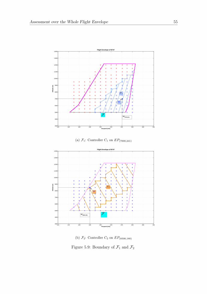
Assessment over the Whole Flight Envelope 55
120 140 160 180 200 220 240 260 280 3003000
4000
5000
6000
7000
8000
9000
10000
11000
12000
13000
14000
Airspeed (m/s)
Alti
tude
(m
)
Flight Envelope of B747
EP(7000,241)
C1
F
F1
(a) F1: Controller C1 on EP(7000,241)
120 140 160 180 200 220 240 260 280 3003000
4000
5000
6000
7000
8000
9000
10000
11000
12000
13000
14000
Airspeed (m/s)
Alti
tude
(m
)
Flight Envelope of B747
FEP(8500,180)
F2
C2
(b) F2: Controller C2 on EP(8500,180)
Figure 5.9: Boundary of F1 and F2

56Assessm
entover
theW
hole
Flig
htEnvelo
pe
120 140 160 180 200 220 240 260 280 3003000
4000
5000
6000
7000
8000
9000
10000
11000
12000
13000
14000
Airspeed (m/s)
Alti
tude
(m
)
Flight Envelope of B747
F
F2
C2
EP(7000,241)
C1F1
EP(8500,180)
EP(10500,210)
FG
FH
FG
FH : Uncovered region
: Overlapped region
Figu
re5.10:
FH
andF
G

Assessment over the Whole Flight Envelope 57
0 0.5 1 1.5 2 2.5 3 3.5 4 4.5 50
0.5
1
1.5
2
2.5
Step Response
Time (sec)
Am
plitu
de
Figure 5.11: C∗ criterion assessment of the aircraft with C2 on EP(11500,210)
−40 −20 0 20 40 60 80−2
0
2
4
6
8
10
12
14
16
Pilot Phase Compensation [deg]
Res
onan
ce [d
B]
Tendency to oscillate
Strong PIO tendency
Good responsive airplane
Level 3
Level 1
Phase Lag Phase Lead
Level 2
Figure 5.12: Neal and Smith criterion assessment of C2 on EP(11500,210)

58 Assessment over the Whole Flight Envelope
120 140 160 180 200 220 240 260 280 3003000
4000
5000
6000
7000
8000
9000
10000
11000
12000
13000
14000
X: 180Y: 5000
Airspeed (m/s)
Alti
tude
(m
)
Flight Envelope of B747
X: 200Y: 5000
X: 265.6Y: 1.219e+004
X: 260Y: 8500
F2
F1
F1
F2
F12
F12
F
Figure 5.13: Identification of F with F1 and F2
120 140 160 180 200 220 240 260 280 3003000
4000
5000
6000
7000
8000
9000
10000
11000
12000
13000
14000
Airspeed (m/s)
Alti
tude
(m
)
Flight Envelope of B747
FC12
FC2
FC1
FC12
F
FC1
FC2
F
Figure 5.14: Identification of F with FC1 , FC2 and FC12

Gain Scheduling 59
Chapter 6
Gain Scheduling
In the previous chapters, two sets of longitudinal Rate Command-Attitude Hold(RCAH) controllers C1 and C2 are designed for the linear aircraft models usingpole placement method at the specific equilibrium points. In addition, the handlingqualities of the aircraft are assessed according to the CAP, Neal and Smith, andC∗ criteria over the flight envelope. In this chapter, the gain scheduling techniqueis conducted in interpolation region FC12 with desired response about the schedul-ing parameters. In this thesis, the current value of the airspeed and altitude areconsidered as the main scheduling parameters, against which the controllers’ gainmatrix are scheduled. In other words, the controller gains are smoothly scheduledaccording to the current trimmed operating conditions.
In practice the aircraft dynamic description is nonlinear, such that the flight con-trollers with scheduled gains are essential if they are to be robust enough to providegood performance and endow the aircraft with desirable handling qualities through-out the flight envelope. Since the operating region FC1 , FC2 and FC12 are determinedbased on the handling qualities assessment, the nonlinear control problem is sub-divided into a series of linear ones. C1 and C2 are designed based on two statesof the scheduling parameters: EP(7000,241) and EP(8500,180). This ensures that eachcontroller gain matrix is set for the current equilibrium point to suit each lineardesign condition, and therefore provides a performance that is close to optimal.For interpolation region FC12 , gains are calculated at specific equilibrium operatingpoints with a certain scheduling strategy, which results in a controller that givesthe desired performance about trimmed operating conditions. Consequently, a setof controllers is reconstructed by combining members of the Linear Time Invariant(LTI) local controllers.
6.1 Gain Scheduling Factor
In order to transit smoothly from one flight controller to another, a strategy of gainscheduling which is a continuous function of scheduling variables ( VTAS and he), is

60 Gain Scheduling
needed to meet a desired performance and handling qualities specification.
The gain scheduling strategy is expressed as,
Ki = K1e+K2(1− e) (6.1)
where:
• Ki is scheduled gain matrix.
• K1 and K2 are matrices of the gains of C1 and C2 respectively. The values canbe obtained from Table 5.1.
• Parameter e is the gain scheduling factor where e ∈ [0, 1], and e varies accord-ing to the current value of the scheduling variables e = f(VTAS, he), where(VTAS, he) ∈ FC12 , which is shown in Fig. 6.1 and Fig. 6.2.
140 160 180 200 220 240 260 2805000
6000
7000
8000
9000
10000
11000
12000
13000
Airspeed VTAS (m/s)
Altitude
he
(m)
Figure 6.1: Gain scheduling factor along with the B747 flight envelope-2D
Fig. 6.1 and Fig. 6.2 show the surface where the gain scheduling factor e is inter-polated linearly. The region FC12 is interpolated at operating points specified bythe current VTAS and he to produce the gain scheduling factor e. The program ispresented in Appendix D
6.2 Scheduled Gain Matrices
In this section, a set of typical equilibrium points are chosen to verify the gainscheduling strategy in FC12 .

Gain Scheduling 61
140160
180200
220240
260280
5000
6000
7000
8000
9000
10000
11000
12000
13000
0
0.1
0.2
0.3
0.4
0.5
0.6
0.7
0.8
0.9
1
Airspeed VTAS (m/s)
Altitude he (m)
Gain
sched
uling
fact
or
e
Figure 6.2: Gain scheduling factor along with the B747 flight envelope-3D
6.2.1 Gain Matrix
Equilibrium points EP(5500,200), EP(8000,230) and EP(11000,260) are chosen to representthe extremity and middle properties of the scheduler in FC12 , see Fig. 6.3.
With reference to the relationship defined in the equation (6.1), the scheduled gainmatrix on EP(5500,200), EP(8000,230) and EP(11000,260) are calculated as follows.
Ki = K2e+K1(1− e) (6.2)
where,
K1 =[
kq kα kǫq m]
(6.3)
=[
0.73 −1.67 2.87 1.60]
(6.4)
K2 =[
1.68 −3.33 5.76 3.84]
(6.5)
hence,
e(5500,200) = 0.4286 (6.6)
K(5500,200) =[
1.10 −2.32 4.01 2.48]
(6.7)
e(8000,230) = 0.6237 (6.8)
K(8000,230) =[
1.30 −2.67 4.62 2.96]
(6.9)
e(11000,260) = 0.7652 (6.10)
K(11000,260) =[
1.46 −2.94 5.08 3.31]
(6.11)

62 Gain Scheduling
120 140 160 180 200 220 240 260 280 3003000
4000
5000
6000
7000
8000
9000
10000
11000
12000
13000
14000
Airspeed (m/s)
Alti
tude
(m
)
Flight Envelope of B747
EP(5500,200)
EP(8000,230)
EP(11000,260)
F
FC1
FC2
FC12
Figure 6.3: Equilibrium points EP(5500,200), EP(8000,230) and EP(11000,260) in FC12
Fig. 6.4 shows how the gains vary as transit through equilibrium points EP(5500,200),EP(8000,230) and EP(11000,260).
6.2.2 Performance
For the equilibrium points EP(5500,200), EP(8000,230) and EP(11000,260), the open loopand closed loop system characteristic polynomials are obtained as follows. Notethat the closed loop system characteristic polynomials are derived from the aircraftmodel augmented by scheduled gains from equations (6.7), (6.9) and (6.11).
∆(s)(5500,200)open = (s+ 0.00001)(s2 + 0.003s+ 0.006)(s2 + 1.18s+ 1.47) (6.12)
∆(s)(5500,200)close = s(s+ 2.136)(s+ 0.0058)(s2 + 2.777s+ 3.36) (6.13)
∆(s)(8000,230)open = (s+ 0.0004)(s2 + 0.0026s+ 0.0034)(s2 + 1.08s+ 1.38) (6.14)
∆(s)(8000,230)close = s(s+ 3.182)(s+ 0.0053)(s2 + 2.628s+ 2.366) (6.15)
∆(s)(11000,260)open = (s+ 0.01)(s2 + 0.008s+ 0.002)(s2 + 0.99s+ 1.35) (6.16)
∆(s)(11000,260)close = s(s+ 3.565)(s+ 0.0214)(s2 + 2.569s+ 1.913) (6.17)
The characteristics of the longitudinal dynamics, which are characterized by theShort-Period Pitching Oscillation (SPPO) mode and phugoid oscillation mode, arerepresented by the second order oscillatory factors in the open loop at three equilib-rium points EP(5500,200), EP(8000,230) and EP(11000,260). The short period mode andthe phugoid mode of the basic aircraft exhibit classical, second-order characteris-

Gain Scheduling 63
EP (5500,200) EP (8000,230) EP (11000,260)−3
−2
−1
0
1
2
3
4
5
6
Eqilibrium points
Gai
ns
Kq
Kεq
Kα
M
Figure 6.4: Scheduled gains of
tic which are modified considerably for the augmented aircraft. The following twoaspects are discussed.
• For the short period mode, the natural frequency is decreased together with asmaller reduction in the damping ratio for the increasing altitude and airspeedin the open loop. While the short period mode is substantially modified bythe scheduler in the closed loop. It is clear that the design objectives ofexact integral pole-zero cancellation can not be achieved by the schedulerdesigned upon each equilibrium point, which is also the general case in a realapplication. Hence, the integral lag time constant term is inevitably inducedinto the system. According to equations (6.13), (6.15) and (6.17), the integrallag time constants on EP(5500,200), EP(8000,230) and EP(11000,260) are given by,
Tlag(5500,200) =1
2.136= 0.468s (6.18)
Tlag(8000,230) =1
3.182= 0.314s (6.19)
Tlag(11000,260) =1
3.565= 0.281s (6.20)
It indicates the integral lag time constants decrease with increasing airspeedand altitude, which means the aircraft response becomes more responsive topilot control. 0.468s is the maximum value in equation (6.18), which is stilladequately small, and is not especially obvious to the pilot. However, since

64 Gain Scheduling
it is still likely to induce an intrusive handling qualities problem, the han-dling qualities of the aircraft with scheduled gains of K(5500,200), K(8000,230) andK(11000,260) in region FC12 are assessed in the following section.
• For the phugoid mode, it is represented by a pair of stable poles and a secondorder oscillation for the basic aircraft in the open loop. The natural frequencyof the phugoid mode is slightly reduced with increasing altitude and airspeed.In the closed loop, the mode is no longer oscillatory and is represented by astable and negative pair of real poles. It means that the phugoid tendencyis with a stable long time constant pole, and is not especially obvious to thepilot. The phugoid mode of the basic aircraft is improved considerably by thescheduler.
6.3 Handling Qualities Assessment
A handling qualities assessment is conducted in this section, to evaluate the influenceof the scheduled gains upon the handing qualities of the aircraft in FC12 .
Firstly, the handling qualities of the aircraft augmented by K(5500,200), K(8000,230) andK(11000,260) are assessed respectively based on three equilibrium points, EP(5500,200),EP(8000,230) and EP(11000,260) shown in 6.3. Secondly, an assessment of the aircraftaugmented by scheduled gains is performed over the set of equilibrium points inFC12 .
6.3.1 Assessment On EP(5500,200), EP(8000,230) and EP(11000,260)
The CAP, Neal and Smith, and C∗ criteria are employed to assess the handling qual-ities of the aircraft with scheduled gains on EP(5500,200), EP(8000,230) and EP(11000,260)
shown in Fig. 6.3. The results are presented in Fig. 6.5, Fig. 6.8 and Fig. 6.9.
As can be observed from Fig. 6.5, Fig. 6.8 and Fig. 6.9, a consistent assessment isobtained, which is the aircraft with scheduled gains on EP(5500,200), EP(8000,230) andEP(11000,260) possess satisfactory handling qualities. In particular:
• Firstly, CAP assessment shown in Fig. 6.5 indicates that there is consider-able margin between the minimum CAP value of 0.085 and the closed loopCAP parameters for a Category B flight phase, say CAP(5500,200) = 0.32,CAP(8000,230) = 0.22 and CAP(11000,260) = 0.19.
• Secondly, the pilot and aircraft closed loop system, as shown in Fig. A.1, areplotted on the Bode plot. As pointed out in the Neal and Smith criterionassessment on EP(8000,230) in the Bode plot on Fig. 6.6, the maximum lowfrequency droop is −2 dB which is less than the value −3 dB specified in thecriterion. Comparing with the equilibrium points EP(5500,200) and EP(11000,260),
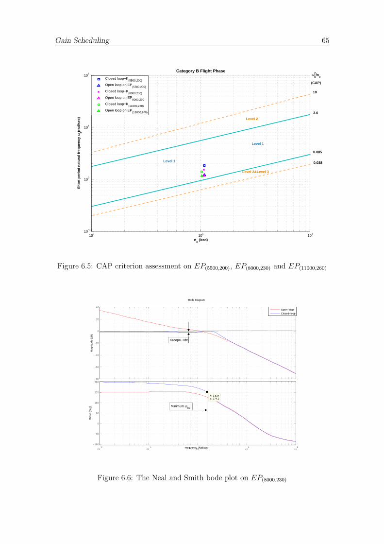
Gain Scheduling 65
100
101
102
10−1
100
101
102
Category B Flight Phase
nα (/rad)
Sho
rt p
erio
d na
tura
l fre
quen
cy
ωs(r
ad/s
ec)
Closed loop−K(5500,200)
Open loop on EP(5500,200)
Closed loop−K(8000,230)
Open loop on EP8000,230
Closed loop−K(11000,260)
Open loop on EP(11000,260)
Level 2
Level 1
Level 1
Level 2&Level 3
ω2s/nα
(CAP)
10
3.6
0.085
0.038
Figure 6.5: CAP criterion assessment on EP(5500,200), EP(8000,230) and EP(11000,260)
−80
−60
−40
−20
0
20
40
Mag
nitu
de (
dB)
10−2
10−1
100
101
102
−180
−90
0
90
180
270
360
X: 1.534Y: 274.2
Pha
se (
deg)
Bode Diagram
Frequency (rad/sec)
Open−loop
Closed−loop
Droop=−2dB
Minimum ωbw
Figure 6.6: The Neal and Smith bode plot on EP(8000,230)

66 Gain Scheduling
−30
−25
−20
−15
−10
−5
0
5
10
Mag
nitu
de (
dB)
10−2
10−1
100
101
102
0
45
90
135
180
225
270
315
360
Pha
se (
deg)
Bode Diagram
Frequency (rad/sec)
Closed loop system model with gain K(5500,200)
Closed loop system model with gain K(8000,230)
Closed loop system model with gain K(11000,260)
Figure 6.7: The Neal and Smith bode plot of closed loop system on 3 EP s
−40 −20 0 20 40 60 80−2
0
2
4
6
8
10
12
14
16
Pilot phase compensation at ω=1.5 rad/s (deg)
Clo
sed
loop
res
onan
ce(d
B)
Level 1Level 2Zero phase compensationClosed loop−K
(5500,200)
Open loop on EP(5500,200)
Closed loop−K(8000,230)
Open loop on EP8000,230
Closed loop−K(11000,260)
Open loop on EP(11000,260)
Phase LeadPhase Lag
Level 3
Level 2
Level 1
Sluggish responseStrong PIO tendency
Tendency to oscillate
Good responsive airplane
Figure 6.8: Neal and Smith criterion assessment against boundary requirement
Gain Scheduling 67
similar assessment results are obtained in Fig. 6.7. Consequently, Level 1handling qualities are predicted by plotting closed loop resonance and pilotphase compensation against the Neal and Smith requirements in Fig. 6.8.
• Thirdly, Fig. 6.9 plots the step response and frequency response against the C∗
criterion requirements for Category C flight phase on EP(5500,200), EP(8000,230)
and EP(11000,260). All of them indicate that the handling qualities of the aircraftwith scheduled gains in the take off and landing flight phase meet the criterionrequirement.
6.3.2 Assessment over Region FC12
The CAP, Neal and Smith criteria are utilized in this section to assess the handlingqualities of the aircraft augmented with scheduled gains over the interpolation regionFC12 .
In order to estimate the influence of the scheduled gains upon the handing qualitiesof the aircraft in FC12 , the scheduled gains on the set of equilibrium points in FC12
are calculated. Based on the gain scheduling factor in equation (6.1), the scheduledgains are calculated according to the value of he and VTAS at each equilibrium point,which are used to augment the aircraft models in FC12 . The augmented aircraftmodels at the set of equilibrium points in FC12 are now obtained. Consequently,the handling qualities assessment of these augmented aircraft models is presentedin Fig. 6.10 and Fig. 6.11.
Fig. 6.10 and Fig. 6.11 indicate the CAP criterion assessment and the Neal andSmith criterion assessment over the region FC12 .
• The CAP assessment predicts Level 1 handling qualities in FC12 . For the air-craft augmented with scheduled gains, the CAP parameters are less marginallylocated in the Level 1 handling qualities requirements for Category B flightphase due to the short period natural frequency ωs and damping ratio ζs beingimproved to compensate the aircraft response to the pilot control.
• The Neal and Smith criterion assessment in FC12 indicates that the aircraftaugmented by scheduled gains are predicted with Level 1 handling qualities,shown in Fig. 6.11.

68 Gain Scheduling
Step Response
Time (sec)
Am
plitu
de
0.5 1 1.5 2 2.5 3 3.5 40
0.5
1
1.5
2
2.5
Boundaries of Flight Phase Category C
C* with gain K(11000,260)
C* with gain K(8000,230)
C* with gain K(5500,200)
(a) C∗ criterion-step response
10−1
100
101
102
−20
−15
−10
−5
0
5
10
15
Mag
nitu
de (
dB)
Bode Diagram
Frequency (rad/sec)
C* with gain K(5500,200)
C* with gain K(8000,230)
C* with gain K(11000,260)
Category 1 envelope−optimum response
( Equivalent to Flight Phase CAT C)
(b) C∗ criterion-frequency response
Figure 6.9: C∗ criterion assessment on EP(5500,200), EP(8000,230) and EP(11000,260)
Gain Scheduling 69
100
101
102
10−1
100
101
102
nα (/rad)
Sho
rt p
erio
d na
tura
l fre
quen
cy
ωs(r
ad/s
ec)
Category B Flight Phase
Level 1
Level 1
ω2s/nα
10
(CAP)
3.6
0.085
0.038
Level 2&Level 3
Level 2
x
Closed loop
Open loop
Figure 6.10: CAP criterion assessment in FC12
−40 −20 0 20 40 60 80−2
0
2
4
6
8
10
12
14
16
Level 3
Level 2
Level 1
Sluggish responseStrong PIO tendency
Tendency to oscillate
Good responsive airplane
Phase Lag Phase Lead
x Open loop
Closed loop
Figure 6.11: The Neal and Smith criterion assessment in FC12

This page intentionally contains only this sentence.
Conclusions 71
Chapter 7
Conclusions
This thesis presents a method for the design and development of gain schedulingcontrollers for a passenger aircraft B747 from the viewpoint of handling qualitiesassessment. Firstly, the state space pole placement design procedure is employedto design the longitudinal Rate Command-Attitude Hold (RCAH) controllers asthe local flight controllers. Secondly, handling qualities of the aircraft augmentedby the local controllers are assessed over the whole flight envelope to identify theinterpolation region FC12 . Finally, the controller gains are scheduled against thecurrent value of the airspeed and altitude in order to obtain smooth transition fromone flight controller to another in different flight conditions. A summary of the keyfindings and suggestions for further work are presented in this chapter.
7.1 Summary of Findings
In this thesis, the key findings comprise three major areas: flight control law design,handling qualities assessment and gain scheduling techniques.
7.1.1 Flight Control Law Design
Two sets of the longitudinal Rate Command Attitude Hold (RCAH) controllersare designed by means of pole-placement design procedure based on the existingBoeing 747-100/200 aircraft model. In order to achieve an attitude hold character-istic, and also improve the dynamic tracking behavior of the aircraft, the classicalproportional-plus-integral (PI) controller structure with pitch rate q and angle ofattack α feedback is implemented. In particular:
• The aircraft model is trimmed and linearized based on the application of theBoeing 747-100/200 aircraft model trim and linearization routine along withthe flight envelope.

72 Conclusions
• The longitudinal flight control law is designed with RCAH characteristics. Itis found that the pitch rate q and angle of attack α feedback to elevator areeffective to modify the longitudinal short period mode stability characteristicsof the aircraft. Kq effectively increases the short period mode damping, andKα increases the short period mode frequency. The values of the pitch-ratefeedback gain Kq, the angle of attack feedback gain Kα, the integrator gainKǫq and the feed-forward gain Km are calculated by placing the short periodpoles at the desired locations on the s-plane.
• The longitudinal Rate Command Attitude Hold (RCAH) controllers endowsthe aircraft with good attitude tracking and handling characteristics due to theapplication of the structure including a classical PI controller; level 1 handlingqualities are accessible for C1 and C2.
• For the local controller C1 and C2, the design objective of minimizing the effectof the time lag introduced by the integral term, is achieved by near exactintegral pole-zero cancellation. Although the integral pole-zero cancellationcan not be achieved at each equilibrium point, the assessment shows the timelag does not induce an intrusive handling qualities problem. Moreover, thisis the general case in a real application, even for the perfect integral pole-zero cancellation design. The integral lag time constant term is inevitablyinduced into the system due to different components in the control loop, suchas actuators.
7.1.2 Handling Qualities Assessment
Utilizing a number of existing flying specifications and handling qualities criteria,the longitudinal handling qualities of the B747 aircraft are assessed over the wholeflight envelope. The key findings are summarized as follows:
• Handling qualities criteria are generally better developed for the military andcombat aircraft.In this thesis, the CAP, Neal and Smith, and C∗ criteria are applied in theB747 aircraft handling qualities assessment. These criteria are developed forthe military and combat aircraft with the explicit purpose of ensuring gooddynamic response characteristics in the execution of the defined flight task ormission. For the handling qualities assessment of a civil passenger aircraft likeB747, the US Federal Aviation Regulations (FAR-25) [Ano94] or CertificationSpecification for Large Aeroplanes (CS-25) [CS206] might be the most suit-able to comply with. Unfortunately, there are few specifications to quantifythe handling qualities in FAR-25 and CS-25. For more formal analytical pur-poses, it is necessary for the handling qualities to be described quantitatively.Although these criteria are generally better developed for the military andcombat aircraft, the CAP, Neal and Smith, and C∗ criteria can still be appliedto assess the handling qualities of the B747 aircraft.

Conclusions 73
• The longitudinal handling qualities of the B747 aircraft are improved by localcontrollers C1 and C2.Comparing the assessment of the basic aircraft with the assessment of theaugmented aircraft using the CAP, Neal and Smith, and C∗ criteria, consistentresults can be obtained, which shows the closed loop flight controller improveshandling qualities of the aircraft considerably. In particular,
1. CAP criterionThe CAP parameter of the augmented aircraft is well inside the boundaryof CAP Level 1 handling qualities requirements. In other words, theaugmented B747 aircraft shows less marginal Level 1 flying qualities thanthe basic aircraft does for a category B (Cruise) flight phase.
2. The Neal and Smith criterionThe Neal and Smith criterion, which is considered as a critical measure ofpilot handling opinion for the pitch tracking task, is then used as the mainmethod to assess the handling qualities of the Rate Command AttitudeHold (RCAH) controllers, and furthermore, to aid in the design of thescheduler.
(a) Handling qualities assessment of the aircraft with C1 and C2 con-trollers at equilibrium design points EP(7000,241) and EP(8500,180)
It is found that for short period mode, an increased natural frequencyeffectively reduced the pilot compensation in order to achieve a closedloop bandwidth of ωBW = 1.5rad/s. Meanwhile, the improvement ofthe damping ratio decreases the closed loop resonance peak consider-ably. Both of these endow the aircraft augmented by controllers C1
and C2 at EP(7000,241) and EP(8500,180) with Level 1 handling qualitiesin the Neal Smith criterion.
(b) Assessment of the aircraft over the flight envelopeFirstly, handling qualities of the aircraft with C1 and C2 are assessedover the flight envelope to identify the operating range FC1 , FC2
and FC12 . It is found that there is general trend towards a predic-tion of degrading handling qualities in the pitch tracking task in lowairspeed and high altitude flight conditions. In addition, superiorhandling qualities are found near the equilibrium point for which thecontroller was designed for, this was to be expected. Secondly, thehandling qualities of the aircraft with the scheduler are assessed inthe interpolation region FC12 . It is found that the Neal and Smithcriterion predicts Level 1 handling qualities of the aircraft with thescheduler in pitch tracking task.
3. C∗ criterionThe step response and the Bode plot of the C∗ transfer function arelocated in the acceptable limits envelope of Flight Phase Category C.It indicates the augmented aircraft possessing the acceptable handlingqualities in takeoff and landing flight phase.

74 Conclusions
7.1.3 Gain Scheduling
A gain scheduling scheme that is a continuous function of the scheduling variables isdesigned. It is found that this scheduling scheme provides continuous and automaticgain-scheduling with respect to VTAS and he, and a desired performance and handlingqualities for the aircraft augmented by the scheduler in the flight envelope assumingfrozen values of scheduling parameters - VTAS and he.
7.2 Recommendations for Further Work
With regards to the further work on the subject, there are several directions thatcould be further researched and developed as grouped into the following categories:flight control, handling qualities and gain scheduling techniques.
7.2.1 Flight Control Law Design
In this thesis, the longitudinal Rate Command-Attitude Hold (RCAH) commandand stability augmentation system is designed to improve longitudinal dynamicmanoeuvring characteristic with the ability to undertake precision pitch attitudetracking. For the purpose of good aircraft stability in all axes, several other controllaws are likely to be interesting topics for the further work.
• Longitudinal control lawC∗ includes a combination of normal acceleration and pitch rate feedback toelevator. A C∗ control law design strategy embodies the desirable dampingaugmentation of pitch rate feedback together with the desirable commandcharacteristics of acceleration feedback.
• Lateral control lawThe lateral roll control law provides a classical roll rate command character-istic since it utilizes roll rate feedback to improve roll damping. The basiccontroller structure is designed to give a rate command attitude hold controlcharacteristic.
• Yaw control lawRate feedback auto-stabilizer, yaw damper with yaw rate feedback can beused to increase the damping of the dutch roll mode. A yaw damper thatutilizes yaw rate feedback to improve dutch roll dynamics and incorporates anaileron-rudder-interlink (ARI) will help minimize side-slip during turn entry.
In addition to the CSAS control law mentioned above, it is increasingly commonto find a Load Alleviation Function (LAF) in many large civil aircraft to improvepassenger ride comfort and reduce structural dynamic deformations by managing

Conclusions 75
manoeuvre and gust loads of the wing [And10]. This aspect is also very interestingfor further work.
7.2.2 Handling Qualities Assessment
• The stability and control characteristics are assumed to be constant through-out the flight envelope in this thesis, and are also one of the essential factorsinfluencing the handling qualities of the aircraft. Hence aircraft stability andcontrol characteristics analysis is an important issue for the practical assess-ment, and this aspect is also very interesting for further work.
• Assessment of handling qualities by flight simulator studies [Cas03].Simulation of the aircraft is required to identify the issues with the param-eter varying nature of the scheduled controller, especially when crossing theboundaries between FC1 , FC2 and FC12 . The contents of the handling qual-ities assessment and performance analysis are extended to the assessment ofthe different flight tasks or flight conditions based on the simulation, such astakeoff, engine failure and crosswind landing configuration.
7.2.3 Gain Scheduling Technique
• Developed tools to aid the identification of the relative scheduling regionThe relative scheduling region presented here is identified based on the analysisof the handling qualities of the aircraft, and the equilibrium points are chosenby means of the heuristic method, the choice of the design points EP couldbe optimized in the future, so that handling qualities are optimized over thewhole flight envelope.
• Advanced gain scheduling methodIn this thesis, the conventional gain scheduling approach is employed to han-dle the nonlinear property of the aircraft, which is successfully and popularlyimplemented in aircraft engineering applications. However, this approach hasshortcomings: expensive, time-consuming and no guarantees on the robust-ness, performance and stability of the overall gain scheduled design. In recentyears, Linear Parameter Varying (LPV) control has been established as anemerging advanced approach to be a reliable alternative to the conventionalgain-scheduling approach [EB01] [Chu10]. LPV is based on the principle ofthe H∞ multi-variable control, and guarantees excellent performance. Gainscheduling using advanced method is an interesting topic for further research.

This page intentionally contains only this sentence.

The Neal and Smith Criterion Assessment 77
Appendix A
The Neal and Smith CriterionAssessment
This section discusses the Neal and Smith criterion assessment for the aircraft.Specifically it covers the routine procedures of the Neal and smith criterion [Coo10a].
A.1 Introduction
For the purpose of applying this criterion to assess the handling qualities of theaircraft, a pilot model transfer function is introduced to construct a ‘pilot and air-craft closed loop system model’ as shown in Fig. A.1. The handling qualities ofthe aircraft, which is determined by the perception of pilot to accomplish a certaintask, is measured in terms of the amount of gain and phase introduced by the ‘pilotand aircraft closed loop system model’ in this situation. The open-loop transferfunction of the pilot model is applied as follows, which includes a pure time delay,gain compensation and phase compensation term.
F (s) = Fp(s) ·θ(s)
δe(s)(A.1)
Fp(s) = Kpe−τs (1 + sTp1)
(1 + sTp2)= KpDp(s)Pp(s) (A.2)
where:
• Kp is pilot gain compensation term.
• Dp(s) is a pure-time delay term of τ seconds. For a typical human pilot, pilotdelay is assumed to be τ = 0.3s. For this analysis, the pilot’s neuromusculardelay is assumed to be a second-order Pade approximation with 0.3s of thecontinuous-time delay e−0.3s in transfer function form. More details will bediscussed in section A.3.1.

78 The Neal and Smith Criterion Assessment
• Pp(s) is phase compensation term.
• Fp(s) is the pilot model.
• F (s) is pilot and aircraft open loop transfer function.
Pilot Model
Fp(s)
ResponseAircraft
(s)
e(s)
d e
(s)
e
Figure A.1: Pilot and aircraft closed loop system model
The pilot and aircraft closed loop system model is shown in Fig. A.1. The handlingqualities are assessed next using the gain and phase characteristics of this pilot andaircraft closed loop system model.
A.2 The criterion
The original criterion definition of the minimum bandwidth frequency is a fixedvalue of 3.5 rad/s [TR71]. This definition is broadened by MIL-STD-1797A [Ano90]into other flight phase categories shown in Table A.1. An minimum bandwidth ofCategory B ωBW = 1.5 rad/s is chosen here. The criterion were developed in terms
Table A.1: Bandwidth requirements of different flight phase[Ano90]
Flight Phase BandwidthCategory A 3.5 rad/sCategory B 1.5 rad/sLanding 2.5 rad/sOther Category C 1.5 rad/s
of limiting values for the handling parameters, the limits are defined as follows,
1. Minimum Bandwidth, ωBW = 1.5 rad/s at Phase = −90 deg.
2. Maximum low frequency, Droop = −3 dB.
3. Closed loop resonance; the best minimum peak value that can be achieved.

The Neal and Smith Criterion Assessment 79
The criterion specifies the minimum closed loop bandwidth (ωBW ) as 1.5 rad/s whenphase lag φ first reaches −90 deg and a maximum low-frequency droop of −3 dB.The low-frequency droop and closed-loop resonance are the main parameters whichdetermine the handling qualities assessment of the aircraft. The boundaries of Level1, Level 2 and Level 3 plotted in Fig. A.6 are for aircraft with the minimum band-width of 3.5 rad/s, and have been generated from empirical data correlation, basedon a certain amount of flight tests of fighter when implementing the pitch trackingtask. The empirical boundaries (for different flight phase categories) determined byflight tests, stipulate a closed-loop droop no more than −3 dB for Levels 1 and 2 andclosed-loop resonance no greater than 3 dB for Level 1 in MIL-STD-1797A [Ano90].Therefore the data do not conflict with the boundaries of Level 1, Level 2 and Level3 for the minimum bandwidth 3.5 rad/s. Consequently, although these boundariesare not quite suitable for the aircraft with the minimum bandwidth of 1.5 rad/s inflight phase category B, they still could be used to rate the handling qualities as areference to illustrate the improvement of the handling qualities from the basic tothe augmented aircraft.
A.3 Open loop
This pilot model transfer function is required for the Neal and Smith criterion appli-cation. The pitch rate response to elevator transfer function derived from equation(3.18) is therefore,
q(s)
δe(s)=kq(s+
1Tθ2
)
∆(s)(A.3)
=4.6099(s+ 0.4905)
(s2 + 1.243s+ 1.58)(A.4)
The pitch attitude response to elevator transfer function follows directly,
θ(s)
δe(s)=kq(s+
1Tθ2
)
s∆(s)(A.5)
=4.6099(s+ 0.4905)
s(s2 + 1.243s+ 1.58)(A.6)
Note that the longitudinal stability characteristics of short period mode are there-fore,
ζs = 0.495, ωs = 1.26rad/s; (A.7)
both of which meet Level 1 requirements of MIL-F-8785C specifications.

80 The Neal and Smith Criterion Assessment
A.3.1 Frequency response of aircraft plus pilot delay
The transfer function is given by,
F (s) = Dp(s) ·θ(s)
δe(s)= e−0.3s θ(s)
δe(s)=e−0.3s4.6099(s+ 0.4905)
s(s2 + 1.243s+ 1.58)(A.8)
Now, the 2nd-order Pade approximation of the continuous-time delay e−0.3s is givenby
Pade =s2 − 20s+ 133.3
s2 + 20s+ 133.3(A.9)
The comparison of Pade with e−0.3s is shown in Fig. A.2. Then, substitute equation
0 0.1 0.2 0.3 0.4 0.5 0.6 0.7−0.5
0
0.5
1
1.5
Time (secs)
Am
plitu
de
100
101
102
−600
−500
−400
−300
−200
−100
0
Frequency (rad/s)
Pha
se (
deg.
)
Phase response
Pade
e−0.3s
Figure A.2: Step and phase responses of the 2nd order Pade
(A.9) into equation (A.8),
F (s) = Pade ·θ(s)
δe(s)=s2 − 20s+ 133.3
s2 + 20s+ 133.3·
4.6099(s+ 0.4905)
s(s2 + 1.243s+ 1.58)(A.10)
From Fig. A.3, in order to bring the 1.5 rad/s point onto the −90 deg closed loopphase boundary and the maximum low frequency droop into coincidence with the−3 dB closed loop gain boundary, further open loop compensation of phase leadrequired can be given by φp = 22.95 deg.

The Neal and Smith Criterion Assessment 81
0 45 90 135 180 225 270 315 360−40
−30
−20
−10
0
10
20
30
40
50
60
6 dB
3 dB
1 dB
0.5 dB
0.25 dB
0 dB
−1 dB
−3 dB
−6 dB
−12 dB
−20 dB
−40 dB
System: h=F(s)=Pade*\theta(s)/\delta_e(s)Gain (dB): 7.77Phase (deg): 206Frequency (rad/sec): 1.5
Nichols Chart
Open−Loop Phase (deg)
Ope
n−Lo
op G
ain
(dB
)
h=F(s)=Pade*θ(s)/δe(s)
Figure A.3: Nichols chart: Aircraft with pilot delay Pade
A.3.2 Pilot Phase Compensation
Since phase lead φp = 22.95 deg is required from the pilot, a lag-lead network isappropriate to the pilot model and has transfer function,
Pp(s) =1 + sTp11 + sTp2
(A.11)
where, Tp1 ≥ Tp2
ωpk =
(
1
Tp1Tp2
)0.5
= 1.5rad/s (A.12)
sinφp =Tp1 − Tp2Tp1 + Tp2
= sin(22.95◦) = 0.39 (A.13)
Solving the equations (A.12),
Tp1 = 0.44sec (A.14)
Tp2 = 1.006sec (A.15)
The pilot phase compensation transfer function is therefore,
Pp(s) =1.006s+ 1
0.4417s+ 1=
2.278(s+ 0.9938)
(s+ 2.264)(A.16)

82 The Neal and Smith Criterion Assessment
0 45 90 135 180 225 270 315 360−40
−30
−20
−10
0
10
20
30
40
50
60
6 dB
3 dB
1 dB
0.5 dB
0.25 dB
0 dB
−1 dB
−3 dB
−6 dB
−12 dB
−20 dB
−40 dB
System: Fullo=F(s)=Pp*Pade*\theta(s)/\delta_e(s)Gain (dB): 11.3Phase (deg): 229Frequency (rad/sec): 1.5
System: h=F(s)=Pade*\theta(s)/\delta_e(s)Gain (dB): 7.77Phase (deg): 206Frequency (rad/sec): 1.5
Nichols Chart
Open−Loop Phase (deg)
Ope
n−Lo
op G
ain
(dB
)
h=F(s)=Pade*θ(s)/δe(s)
Fullo=F(s)=Pp*Pade* θ(s)/δe(s)
Figure A.4: Nichols chart: Aircraft with pilot delay and phase compensation
A.3.3 Fully phase compensated aircraft
The open loop gain and phase characteristics of the basic aircraft is now compensatedwith pilot delay and pilot phase. Fig. A.5 shows the resulting transfer functionplotted on the Nichols chart, the transfer function is given by,
F (s) = Pade · Pp ·θ(s)
δe(s)= Pade ·
10.5013(s+ 0.9938)(s+ 0.4905)
s(s+ 2.264)(s2 + 1.243s+ 1.58)(A.17)
Fig. A.4 shows a gain reduction of −7.47 dB, which is the open loop gain requiredto bring the 1.5 rad/s point onto the −90 deg closed loop phase boundary and tolead Droop coincidence with −3 dB closed loop gain boundary. Therefore, openloop Kpopenloop
= 0.423. This represents the gain Kp required from the pilot and thuscompletes the description of the pilot model for correct compensation according tothe Neal and Smith criterion. The full pilot model (A.1) is therefore,
Fp(s) = KpDp(s)Pp(s) = KpPade ·(1 + sTp1)
(1 + sTp2)(A.18)
F (s) = Fp(s) ·θ(s)
δe(s)= Pade ·
4.4419(s+ 0.9938)(s+ 0.4905)
s(s+ 2.264)(s2 + 1.243s+ 1.58)(A.19)
The gain and phase characteristics of the aircraft model are compensated by the fullpilot model, and is shown in Fig. A.5.

The Neal and Smith Criterion Assessment 83
0 45 90 135 180 225 270 315 360−40
−30
−20
−10
0
10
20
30
40
50
60
6 dB
3 dB
1 dB
0.5 dB
0.25 dB
0 dB
−1 dB
−3 dB
−6 dB
−12 dB
−20 dB
−40 dB
System: Full1o=F(s)=Kp*Pp(s)*Dp(s)*F_A(s)Gain (dB): 3.88Phase (deg): 229Frequency (rad/sec): 1.5
System: h=Dp(s)*F_A(s)Gain (dB): 7.77Phase (deg): 206Frequency (rad/sec): 1.5
System: Fullo=Pp(s)*Dp(s)*F_A(s)Gain (dB): 11.3Phase (deg): 229Frequency (rad/sec): 1.5
Nichols Chart
Open−Loop Phase (deg)
Ope
n−Lo
op G
ain
(dB
)
h=Dp(s)*FA(s)
Fullo=Pp(s)*Dp(s)*FA(s)
Full1o=F(s)=Kp*Pp(s)*Dp(s)*FA(s)
Figure A.5: Nichols chart: Fully compensated aircraft.
A.3.4 Criterion Check
Based on the full pilot compensation model established above, the handling qualitiesof the aircraft can be assessed against the criterion. The following parameters canbe obtained from Fig. A.5:
• Resonance peak (closed loop)=10.4 dB, which is indicated by the fully com-pensated aircraft curve.
• Pilot phase compensation at 1.5 rad/s=22.95 deg
Fig. A.6 indicates that the basic aircraft handling qualities is Level 3 for the flightcondition of he = 7000 m and VTAS = 241 m/s. The aircraft is sluggish with Level3 flying qualities, hence large pilot compensation is required.
A.4 Closed Loop
This pilot model transfer function is required for the Neal and Smith criterion appli-cation. The pitch rate response to elevator transfer function derived from equations

84 The Neal and Smith Criterion Assessment
−40 −20 0 20 40 60 80−2
0
2
4
6
8
10
12
14
16
Pilot Phase Compensation [deg]
Res
onan
ce [d
B]
Tendency to oscillate
Strong PIO tendency
Good responsive airplane
Level 1
Level 3
Level 2
Open Loop
Figure A.6: Neal and Smith criterion assessment for open loop [Coo10a]
(3.34), (3.35) and (3.36) are therefore,
q(s)
δe(s)=kq(s+
1Tθ2
)
∆(s)=
7.3606(s+ 0.4905)
(s2 + 2.85s+ 3.61)(A.20)
θ(s)
δe(s)=
q(s)
sδe(s)=
7.3606(s+ 0.4905)
s(s2 + 2.85s+ 3.61)(A.21)
The longitudinal stability characteristics of short period mode are therefore,
ζs = 0.75, ωs = 1.9rad/s; (A.22)
both of which meet Level 1 requirements of MIL-F-8785C specifications.
A.4.1 Frequency response of aircraft plus pilot delay
The transfer function derived from equation (A.21) is given by,
F (s) = e−0.3s θ(s)
δe(s)=e−0.3s7.3606(s+ 0.4905)
s(s2 + 2.85s+ 3.61)(A.23)
Substituting Pade for e−0.3s,
Pade =s2 − 20s+ 133.3
s2 + 20s+ 133.3(A.24)
F (s) = Pade ·θ(s)
δe(s)=s2 − 20s+ 133.3
s2 + 20s+ 133.3·7.3606(s+ 0.4905)
s(s2 + 2.85s+ 3.61)(A.25)

The Neal and Smith Criterion Assessment 85
As mentioned in section A.4.1, reference to Fig. A.7, the following parameters arerequired in order to bring the 1.5 rad/s point onto the −90 deg closed loop phaseboundary and the maximum low frequency droop to meet the −3 dB closed loopgain boundary, further open loop compensation of phase lag required can be givenby φp = −14.46 deg.
• Gain reduction −6.6 dB
• Phase lag −14.46 deg
0 45 90 135 180 225 270 315 360−40
−30
−20
−10
0
10
20
30
40
50
60
System: de99=F(s)closeloop=Pade*\theta(s)/\delta_e(s)Gain (dB): 4.74Phase (deg): 244Frequency (rad/sec): 1.5
6 dB
3 dB
1 dB
0.5 dB
0.25 dB
0 dB
−1 dB
−3 dB
−6 dB
−12 dB
−20 dB
−40 dB
Nichols Chart
Open−Loop Phase (deg)
Ope
n−Lo
op G
ain
(dB
)
de99=F(s)closeloop=Pade* θ(s)/δe(s)
Figure A.7: Nichols chart: Augmented aircraft compensated with time delay Pade
A.4.2 Pilot Phase Compensation
Since phase lag φp = −14.46deg is required from the pilot, a lag-lead network isappropriate to the pilot model and has transfer function,
Pp(s) =1 + sTp11 + sTp2
(A.26)
where,
ωpk =
(
1
Tp1Tp2
)0.5
= 1.5rad/s (A.27)
sinφp =Tp1 − Tp2Tp1 + Tp2
= sin(−14.46◦) = −0.25 (A.28)

86 The Neal and Smith Criterion Assessment
Solving the equations (A.27),
Tp1 = 0.52sec (A.29)
Tp2 = 0.86sec (A.30)
The pilot phase compensation transfer function is therefore,
Pp(s) =1 + 0.52s
1 + 0.86s=
0.6(s+ 1.936)
s+ 1.162(A.31)
Augmented aircraft with time delay and phase compensation plotted in Nicholschart is shown in Fig. A.8.
0 45 90 135 180 225 270 315 360−40
−30
−20
−10
0
10
20
30
40
50
60
System: de99=F(s)closeloop=Pade*\theta(s)/\delta_e(s)Gain (dB): 4.74Phase (deg): 244Frequency (rad/sec): 1.5
6 dB
3 dB
1 dB
0.5 dB
0.25 dB
0 dB
−1 dB
−3 dB
−6 dB
−12 dB
−20 dB
−40 dB
System: Full=F(s)closeloop=Pp*Pade*\theta(s)/\delta_e(s)Gain (dB): 2.53Phase (deg): 229Frequency (rad/sec): 1.5
Nichols Chart
Open−Loop Phase (deg)
Ope
n−Lo
op G
ain
(dB
)
de99=F(s)closeloop=Pade* θ(s)/δe(s)
Full=F(s)closeloop=Pp*Pade* θ(s)/δe(s)
Figure A.8: Augmented aircraft with pilot time delay and phase compensation.
A.4.3 Fully phase compensated aircraft
Based on the open loop gain and phase characteristic of the augmented aircraftwith pilot delay and pilot phase compensation discussed in the previous section, thefollowing transfer function can now be obtained,
F (s) = Dp · Pp ·θ(s)
δe(s)= Pade ·
4.4192(s+ 1.936)(s+ 0.4905)
s(s+ 1.162)(s2 + 2.85s+ 3.61)(A.32)
Applying the method described in section A.3.3, Fig. A.8 shows that gain reductionis −5.12 dB, therefore, Kp = 0.5548. This parameter represents the gainKp requiredfrom the pilot and thus completes the description of the pilot model. The final gainand phase characteristics of the augmented aircraft compensated with full pilot

The Neal and Smith Criterion Assessment 87
0 45 90 135 180 225 270 315 360−40
−30
−20
−10
0
10
20
30
40
50
60
6 dB
3 dB
1 dB
0.5 dB
0.25 dB
0 dB
−1 dB
−3 dB
−6 dB
−12 dB
−20 dB
−40 dB
System: de99=Dp(s)*F_A(s)Gain (dB): 4.74Phase (deg): 244Frequency (rad/sec): 1.5
System: Full=Pp(s)*Dp(s)*F_A(s)Gain (dB): 2.53Phase (deg): 229Frequency (rad/sec): 1.5
System: Full1=F(s)=Kp*Pp(s)*Dp(s)*F_A(s)Gain (dB): −2.59Phase (deg): 229Frequency (rad/sec): 1.5
Nichols Chart
Open−Loop Phase (deg)
Ope
n−Lo
op G
ain
(dB
)
de99=Dp(s)*FA(s)
Full=Pp(s)*Dp(s)*FA(s)
Full1=F(s)=Kp*Pp(s)*Dp(s)*FA(s)
Figure A.9: Nichols chart: Fully compensated of augmented aircraft
model are plotted in Nichols chart in Fig. A.9, and Fig. A.10 shows the Neal andSmith assessment comparison against the criterion. The full pilot model open looptransfer function (A.18) is therefore,
Fp(s) = KpDp(s)Pp(s) (A.33)
F (s) = Fp(s) ∗θ(s)
δe(s)= Pade ·
2.4517(s+ 1.936)(s+ 0.4905)
s(s+ 1.162)(s2 + 2.85s+ 3.61)(A.34)
Fig. A.10 indicates that for short period mode, an increased natural frequencyfrom 1.26 rad/s to 1.9 rad/s effectively reduced the pilot compensation in order toachieve a closed loop bandwidth of ωBW = 1.5 rad/s. Meanwhile, the improvementof damping ratio from 0.495 to 0.75 decreases the closed loop resonance peak im-mensely. Both of these endow the aircraft with the Level 1 handling qualities in theNeal and Smith Criterion.

88 The Neal and Smith Criterion Assessment
−40 −20 0 20 40 60 80−2
0
2
4
6
8
10
12
14
16
Pilot Phase Compensation [deg]
Res
onan
ce [d
B]
Level 2
Level 3
Tendency to oscillate
Good responsive airplane
Open loop
Level 1
Strong PIO tendency
Close loop
Figure A.10: Neal and Smith criterion assessment comparison [Coo10a]
Controller C2 Design 89
Appendix B
Controller C2 Design
B.1 Full Order of Equations of Motion
The aircraft model on operating point EP(8500,180) can be obtained following thetrim and linearization routine procedure in section 3.2, which is given by,
x(t) = A2x(t) + B2u(t) (B.1)
where,
x(t) =[
qbody VTAS α θ]T
; (B.2)
u(t) =[
δstab δe]T
(B.3)
A2 =
−0.4390 0.0003 −0.3940 0−0.2191 −0.0087 2.0843 −9.78031.0019 −0.0006 −0.3590 0
1 0 0 0
(B.4)
B2 =
1.4054 2.15950 0
0.0366 0.05890 0
(B.5)
Thus the open loop characteristic polynomial can be obtained by,
∆(s)2 = (s2 + 0.003877s+ 0.007748)(s2 + 0.8024s+ 0.5505) (B.6)
The longitudinal stability modes characteristics are therefore,
ζp = 0.022, ωp = 0.088rad/s; (B.7)
ζs = 0.541, ωs = 0.724rad/s; (B.8)
Normal load factor per unit angle of attack nα2 on operating point EP(8500,180) iscalculated as follows.
nα2 =nz
α= −
zw2Ue
g= −
−0.359× 180
9.8= 6.59g/rad (B.9)

90 Controller C2 Design
where, zw2 can be obtained from the A2 matrix in equation (B.4) by zw2 = zα2 =A2(3,3) = −0.359, and Ue in this case equal to 180m/s.
B.2 Reduced Order of Motion Equations
By decoupling the full order equations of longitudinal motion (B.1), the reducedorder equations of motion of aircraft short period mode can be obtained by,
[
qα
]
=
[
−0.4390 −0.39401.0019 −0.3590
] [
qα
]
+
[
2.15950.0589
]
δe (B.10)
The reduced order transfer functions can be given as follows, by taking the Laplacetransform of equation (B.10):
q(s)
δe(s)=
2.1595(s+ 0.3482)
(s2 + 0.7979s+ 0.5523)(B.11)
α(s)
δe(s)=
0.058889(s+ 37.18)
(s2 + 0.7979s+ 0.5523)(B.12)
The longitudinal stability characteristics of the short period mode are therefore,
ζs = 0.537, ωs = 0.743rad/s; (B.13)
B.3 Control Law of C2
The pole replacement routine is performed as described in sections 3.5.1, 3.5.2 and3.5.3. Before C2 can be designed, the initial design decisions of the desirable locationsof the short period poles on the s-plane are made. The target region F2 requiredto be covered by C2 is with less airspeed and higher altitude than F1. Accordingto the handling qualities assessment in Fig. 5.2, the aircraft in less airspeed andhigher altitude operating conditions, like F2, requires more damping to reduce theclosed loop resonance as well as less response speed and settling time. Comparingwith the design decisions made for C1 design in section 3.5.2, ζsr1 = 0.75, ωsr1 = 1.9and Tlagr1 = 1.8, the stability characteristics of the augmented aircraft by C2 onEP(8500,180), are adjusted into ζsr2 = 0.8, ωsr2 = 1.7 and Tlagr2 = 1.5.
The required closed loop characteristic polynomial of C2 is thus given by,
∆(s) = (s+ 1.5)(s2 + 2.72s+ 2.89) (B.14)
Hence, the control law of C2 is given by,
δe = −[
1.6755 −3.3302 5.7649]
qαǫq
+ 3.8433 · qd (B.15)

Controller C2 Design 91
Substituting equation (B.15) into equation (B.10) the reduced order closed loopstate equation is given by,
qαǫq
=
−4.057 6.797 −12.450.9033 −0.1628 −0.3395
1 0 0
qαǫq
+
8.2990.2263−1
qd (B.16)
The reduced order augmented aircraft transfer functions are obtained as follows, bytaking the Laplace transform of equation (B.16).
q(s)
qd(s)=
8.2995(s+ 0.3482)
(s2 + 2.72s+ 2.89)(B.17)
α(s)
qd(s)=
0.22633(s+ 37.18)
(s2 + 2.72s+ 2.89)(B.18)
ǫq(s)
qd(s)=
−(s− 5.579)
(s2 + 2.72s+ 2.89)(B.19)
For the full order of equations of motion, the C2 control law is given by,
δe = −[
kq kVTASkα kθ kǫq
]
qVTAS
αθǫq
+mqd (B.20)
= −[
1.6755 0 −3.3302 0 5.7649]
qVTAS
αθǫq
+ 3.8433 · qd (B.21)

This page intentionally contains only this sentence.

B747 AIRCRAFT MODEL-FTLAB747v6.5 93
Appendix C
B747 AIRCRAFTMODEL-FTLAB747v6.5
Figure C.1: FTLAB747v6.5 main menu screen
FTLAB747v6.5 is a very powerful aircraft simulation and analysis tool. Based inMatlab/Simulink, the program can be used for simulation and design respectively,

94 B747 AIRCRAFT MODEL-FTLAB747v6.5
and offers a wide array of analysis tools, such as trim, linearisation, flight visualiza-tion and fault detection. In order to take full advantage of this program, much morework is needed to learn the program. It is recommended to read the DASMAT man-ual [vdL96], and the FTLAB747v6.5 manual in Chapter 6 of [EB03], where the trimand linearization routines of FTLAB747v6.5 are presented through a step by stepdescription of the user-supplied data and screen displays. For a specified aircraftconfiguration at a given operating point, a steady-state flight-condition is generatedin aid of the trimming and linearization tools of this program. The original trim-ming and linearization tools are provided in the MATLAB M-scripts ‘trim ac.m’and‘lin ac.m’ respectively. The files ‘trim ac Modified’ and ‘lin ac Modified’ is pro-vided with this thesis, which indicates the change made to the origin software tomeet the requirements of trimming and linearizing the aircraft model over the flightenvelope in this project for applying, and also shows the inherent trimming and thelinearizing routine procedure of the software for analysis.
Each observation group has a different number and type of output parameters. Foractual broad applications, observation outputs are provided by selecting the specificparameters desired in the operating shell, a further description to the individualobservations is given in reference [vdL96] and [EB03]. The symbol of the parameterschosen in this thesis are listed in Table C.1.
Table C.1: Trimming and linearisation Parameters
Symbols Parameters Unitsdelta c δc Column deflection raddelta w δw Wheel deflection raddelta p δp Pedal deflection radPLA engine power lever angle raddelta stab δstab Stablilizer knob raddelta sbh δsbh speedbrake handle raddelta fh δfh flap handle radgear the gear control raddelta eil δeil left inboard elevator raddelta eir δeir right inboard elevator raddelta eol δeol left outboard elevator raddelta eor δeor right outboard elevator raddelta ail δail left inboard aileron raddelta air δair right inboard aileron raddelta aol δaol left outboard aileron raddelta aor δaor right outboard aileron raddelta ih δih horizontal stabilizer raddelta ru δru upper rudder raddelta rl δrl lower rudder radTn engine thrust Nx x aircraft state variables -xdot x aircraft state derivatives -

B747 AIRCRAFT MODEL-FTLAB747v6.5 95
pbdot ˙pbody roll acceleration about body X-axis rad/s3
qbdot ˙qbody pitch acceleration about body Y-axis rad/s3
rbdot ˙rbody yaw acceleration about body Z-axis rad/s3
VTASdot ˙VTAS time derivative of true airspeed m/s2
alphadot α angle of attack rate rad/s
betadot β angle of sideslip rate rad/s
phidot φ roll attitude rate rad/s
thetadot θ pitch attitude rate rad/s
psidot ψ heading rate rad/s
hedot he geometric altitude rate m/sxedot xe horizontal ground speed along earth X-axis m/syedot ye horizontal ground speed along earth Y-axis m/syair yair airdata parameters -yacc yacc acceleration parameters gyfp yfp flight-path-related parameters -ys ys energy-related tems -ypqr ypqr angular axis velocities rad/syuvw yuvw linear axis velocities m/syuvwdot yuvw linear axis velocity derivatives m/s2
ydl ydl dimensionless axis velocities -yabh yαβh sensor measurements -yCaero yCaero
aerodynamic force and moment coeffieients -yFMaero yFMaero
aerodynamic forces and moments -yCgust yCg
force and moment coefficients due to turbulence -yFMgust yFMg
force and moments due to turbulence -yCt yCt
Propulsion force and moment coefficients -yFMt yFMt
propulsion forces and moments m/sygrav ygr gravity forces N

This page intentionally contains only this sentence.

MATLAB Program 97
Appendix D
MATLAB Program
The aircraft model itself is implemented in MATLAB, incorporating a number ofuser-defined functions, as well as existing blocks from the standard Simulink. Ini-tialization and post-processing MATLAB scripts and functions are included for trimand linearisation of the model. the definition of all input parameters. is provided.
This appendix includes a description of the provided MATLAB initialization andpost-processing scripts and functions (including a definition of the required inputsand outputs); a description of the required workspace variables and their correctformat; a brief introduction to the provided Simulink models and libraries; and anoverview of the Simulink model subsystems. Additional documentation is providedwithin the MATLAB program.
D.1 Gain Scheduling Factor Calculation
%===================================================================
% GAIN SCHEDULING FACTOR CALCULATIONS
%===================================================================
%
% Script Name : schedule.m
% Function Name : alpha = schedule(h,v)
%
% Purpose : Calculate the gain scheduling factor alpha against the
% flight conditions at altitude, h, and airspeed, v.
%
% Inputs to the program :
%
% h = Altitude [m]
% v = Airspeed [m/s]
%
% Outputs of the program:

98 MATLAB Program
%
% alpha = gain scheduling factor [-]
%
%
% Subroutines used :
%
% griddata: ZI = griddata(x,y,z,XI,YI,’linear’) fits a surface of the
% form z = f(x,y) to the data in the (usually) nonuniformly spaced
% vectors (x,y,z). ’griddata’ interpolates this surface at the points
% specified by (XI,YI) to produce ZI. The surface always passes through
% the data points. XI and YI usually form a uniform grid (as produced
% by meshgrid). The specified interpolation method ’linear’:
% Triangle-based linear interpolation.
% %====================================================================
function alpha=schedule(h,v)
% Identify the region of the flight envelope F.
% ----------------------------------
if (((h <=12200)&&(h>=5000)&&(((68.5*v-4727-h)>0 ) ||((126.96*v-13963.76-h)>0))
&&... ((343.43*v-80791-h)<=0)&&((182.67*v-40118.67-h)<0)) =1)
% The input flight conditions are not located in the Flight Envelope F.
alpha=NaN;
% Identify the interpolation region Fc12
% ----------------------------------
elseif ((5000<=h<=12200)&& ((58.33*v-6666.7-h)<=0)&&((84.59*v-10226-h)>=0)
)
h1=5000;V1=180; h2=12190;V2=265; h3=8500;V3=260; h4=5000;V4=200;
H0=[h1,h2,h3,h4]; V0=[V1,V2,V3,V4];
% identify the boundary of the interpolation.
alpha0=[1 1 0 0];
% max and min alpha at corners of interpolation
alpha=griddata(H0,V0,alpha0,h,v);
% Calculate the gain scheduling factor.
% Identify the region Fc2
% ----------------------------------
elseif ((5000<=h<=12200)&&(((68.5*v-4727-h)>=0 ) ||((126.96*v-13963.76-h)>=0))
&&... ((84.59*v-10226-h)<=0))

MATLAB Program 99
% C2=[kq,kalpha,Keq,m]
alpha=1;
% Identify the region Fc1
% ----------------------------------
elseif((5000<=h<=8510)&& ((58.33*v-6666.7-h)>0 ) &&((343.43*v-80791-h)<0)
&&... ((182.67*v-40118.67-h)<0))
% C1=[kq,kalpha,Keq,m]
alpha=0;
else
alpha=NaN;
% error(’Inputs are out of the range.’)
end
end
%====================================================================
D.2 Interpolation
%===================================================================
% INTERPOLATION
%===================================================================
%
% Script Name : interpolation.m
%
% Purpose : Schedule the gain matrices according to the scheduling
% parameters (altitude h, and airspeed, v).
%
% Inputs to the program :----------
%
% Outputs of the program:----------
%
% sub program : schedule.m
%
%==================================================================
close all

100 MATLAB Program
clear
h=[5000:50:12200];
% Altitude.
v=[140:1:265];
% Airspeed.
K1=[0.73 -1.67 2.87 1.60];
% Gain matrix of Controller C1.
K2=[1.68 -3.33 5.76 3.84];
% Gain matrix of Controller C2.
for i=1:size(h,2)
for j=1:size(v,2)
ALPHA(i,j)=schedule(h(i),v(j));
% Implementing Function schedule.m .
K(:,:,i,j)=K1*ALPHA(i,j)+K2*(1-ALPHA(i,j));
% The gain scheduling strategy.
end
end
%====================================================================
D.3 The Neal and Smith Criterion Assessment
over the Flight Envelope
%=======================================================================
% The Neal and Smith Criterion Assessment over the Whole Flight Envelope
%=======================================================================
%
%
%==============
% INPUT DATA:
%==============
%
%
% altitude = Altitude [m]
% V0 = Airspeed [m/s]

MATLAB Program 101
% Vco = Cross over velocity [m/s]
% l = cg to pilot distance [m]
% lag = The integral lag time constant [-]
% k = Gain Matrix [kq ka kcq] [rad/rad/s rad/rad/s rad/rad/s]
% BW= 1.5 [rad/s]
%
%==========================
% State Space Matrices
%==========================
%
% Alin,Blin,Clin,Dlin :the full order system.
% As,Bs,Cs,Ds : the reduced order system.
%
%
%==========================
% Transfer Function
%==========================
% Gkm is reduced order of augmented aircraft model.
% G is full order of augmented aircraft model.
% Gs is reduced order transfer function of basic aircraft model.
%
%
%
% Subroutines used :
%
% importfile.m
% createfigurens.m
%=======================================================================
%
altitude=[5000,5500,6000,6500,7000,7500,8000,8500,9000,9500,10000,10500,11000];
V0=[160,150,170,180,190,200,210,220,230,241,250,260];
for i = altitude
for j = V0
importfile([’model ’,num2str(i),’ ’,num2str(j),’.lin’]);
% short period mode
%=================================================================
g=9.8;
V=Alin(5,4); %the current airspeed.
Vco=122; % m/s
l=30; % m,the distance from the pilot station to the 25% MAC as found in
NASA-CR-1756.

102 MATLAB Program
% Reduced Order State Space Matrix of basic aircraft
%-----------------------------------------------------------------------
As=[Alin(1,1) Alin(1,3) 0; Alin(3,1) Alin(3,3) 0; 1 0 0 ];
Bs=[Blin(1,2); Blin(3,2); 0];
Cs=eye(3,3);
Ds=zeros(3,1);
Gs=ss(As,Bs,Cs,Ds); % Reduced order transfer function of basic aircraft
model.
% Designing the Gain Matrix K
%------------------------------------------------------------------------
A1=As-Bs*k;
Gclos=ss(A1,Bs,Cs,Ds); % augmented with k.
zpk(Gclos);
% Designing the Feedforward Gain Matrix M
%------------------------------------------------------------------------
N=[0;0;-1];
kcq=k(1,3);
m=kcq/lag;
B1=Bs*m+N;
Gkm=ss(A1,B1,Cs,Ds);% reduced order of augmented aircraft model.
% controller checked in full order transfer function.
%------------------------------------------------------------------------
A=[Alin(1:4,1:4),zeros(4,1);1,0,0,0,0];
B=[Blin(1:4,2);0];
N=[0;0;0;0;-1];
K=[k(1,1) 0 k(1,2) 0 k(1,3)];
M=m;
A1=A-B*(K);
B1=B*M+N;
C=eye(5,5);
D=zeros(5,1);
G=ss(A1,B1,C,D);% augmented full order aircraft transfer function.
% THE NEAL AND SMITH CRITERION ASSESSMENT
%=======================================================================
% Frequency response of aircraft plus pilot delay
%-----------------------------------------------------------------------

MATLAB Program 103
s=tf(’s’);
[c,d] = pade(0.3,2);
u1=tf(c,d);
de99=minreal(zpk(Gkm(1,1))/s)*u1;
%closed loop Frequency response of aircraft plus pilot delay - ’pade*Gkm’.
h=zpk(Gs(1,1))/s*u1;
% open loop Frequency response of aircraft plus pilot delay- ’pade*Gs’.
[mag1,phase1]=bode(h,1.5);
[mag2,phase2]=bode(de99,1.5);
% Obtain the maginitude and Phase from the Bode Chart when frequency is
1.5 rad/s.
co90=-130.7;
% open loop phase is -130.7deg when closed loop phase is -90deg, in reference
to Flying Qualities and Flight Control Lecture Notes.
ga90=-3.78;
% open loop gain is -3.78dB when closed loop gain is -3dB, in reference
to Flying Qualities and Flight Control Lecture Notes.
Xcriopen=co90-phase1+360
% the required further open loop compensation of phase lead, in order to
bring the 1.5 rad/s point onto the -90 deg closed loop phase boundary and
the maximum low frequency droop into coincidence with the -3 dB closed
loop gain boundary.
co1=sin(Xcriopen*pi/180);
% is used to calculate the parameters of the lag-lead network for basic
aircraft system.
Xcriclos=co90-phase2+360
co=sin(Xcriclos*pi/180);
% used to calculate the parameters of the lag-lead network for augmented
aircraft system.
% Pilot Phase Compensation
%-----------------------------------------------------------------------

104 MATLAB Program
BW=1.5; % Bandwidth
To2=((1+co1)/(1-co1))∧0.5/BW;
To1=(1-co1)/(1+co1)*To2;
Ppo=tf([To2,1],[To1,1]);
% lag-lead network of Pilot phase compensation
Fullo=zpk(Ppo*h);
% Open-loop system with Pilot Phase Compensation
T2=((1+co)/(1-co))∧0.5/BW;
T1=(1-co)/(1+co)*T2;
Pp=tf([T2,1],[T1,1]);
Full=zpk(Pp*de99);% Closed-loop system with Pilot Phase Compensation
%Fully phase compensated aircraft
%-----------------------------------------------------------------------
[mag3,phase3]=bode(Fullo,1.5);
[mag4,phase4]=bode(Full,1.5);
% The required gain reduction in order to bring the 1.5 rad/s point onto
the -90 deg closed loop phase boundary and the maximum low frequency droop
to meet the -3 dB closed loop.
% gain boundary
gao=ga90-mag3; % open-loop
ga=ga90-mag4; % closed-loop
Kpo= 10∧(gao/20);
Kp= 10∧(ga/20);
%Gain in dB=20log10(gain ratio)
Full1=zpk(Kp*Pp*de99);
% the basic aircraft system compensated by the full pilot model.
Full1o=zpk(Kpo*Ppo*h);
% the augmented aircraft system compensated by the full pilot model.
Full2=feedback(Full1,1);
% Full2 is the closed-loop of Full1.
Full2o=feedback(Full1o,1);
% Full2o is the closed-loop of Full1o.

MATLAB Program 105
[mag,phase]=bode(Full2o);
res o=max(20*log10(mag))
% Resonance peak of the basic aircraft system compensated by the full pilot
model Full1.
[magc,phasec]=bode(Full2);
res c=max(20*log10(magc))
% Resonance peak of the basic aircraft system compensated by the full pilot
model Full2.
% PLOTTING
%========================================================================
% Boundaries
%-----------------------------------------------------------------------
Level1 phase=[-30,-15,15,43,50];
Level1 res=[-2,3,3,1.8,-2];
Level3 phase=[-40,0,80];
Level3 res=[11,11,7];
naut phase=[0,0];
naut res=[-2,16];
createfigurens(1,1,2,2,3,3)
title([’model-’,num2str(i),’-V’,num2str(j)]);
plot(Level1 phase,Level1 res,’LineWidth’,2)
hold on;
plot(Level3 phase,Level3 res,’r’,’LineWidth’,2)
hold on;
plot(naut phase, naut res,’c’)
% POINTS
%-----------------------------------------------------------------------
hold on;
plot(Xcriclos,res c,’bo’,Xcriopen,res o,’rx’,’LineWidth’,2)
grid on;
end
end
%=======================================================================

This page intentionally contains only this sentence.
REFERENCES 107
References
[ABB02] N. Aouf, B. Boulet, and R. Botez. A gain scheduling approach for aflexible aircraft. In Proceedings of the American Control Conference,pages 4439–4442, Anchorage AK, May 2002.
[AEJ08] N. M. Ali, R. S. Ehsan, and M. R. Jahed. Aircraft controller designto enhance longitudinal maneuvers. In Proceedings of the 27th ChineseControl Conference, pages 258–264, Kunming,Yunnan, China, July 2008.
[And10] S. P. Andrews. Modelling and Simulation of Flexible Aircraft: HandlingQualities with Active Load Control. PhD thesis, Cranfield University,July 2010.
[Ano80] Anon. Military specification-flying qualities of piloted aircraft. TechnicalReport MIL-F-8785, Department of Defense Military Specifications andStandards, 1980.
[Ano90] Anon. Department of defense interface standard-flying qualities of pi-loted airplanes. Technical Report MIL-STD-1797A, Department of De-fense Military Specifications and Standards, January 1990.
[Ano94] Anon. Federal aviation regulations - part 25, subpart b - flight. Technicalreport, Federal Aviation Administration, United States Department ofTransportation,, 1994.
[ARS01] M. Attar, K. Rosenberg, and H. Smaili. Affordable digital flight controlsystem for small commercial aircraft - adfcs. Air & Space Europe, 3(3-4):184–187, May-August 2001.
[B74] http://www.airliners.net/photo/USA—Air/Boeing-E-4B-(747-200B)/1885779/L/.
[B7407] 747 specifications. Technical Report Retrieved 16, The Boeing Company,December 2007.
[BP02] D. Bates and I. Postlethwaite. Robust Multivariable Control of AerospaceSystems. Delftse University Press, January 2002.
[Cas03] H. V. D. Castro. Flying and Handling Qualities of a Fly-by-wire Blended-Wing-Body Civil Transport Aircraft. Phd thesis, Cranfield University,December 2003.
108 REFERENCES
[Chu10] S Chumalee. Robust Gain-scheduled H∞ Control for Unmanned AerialVehicles. PhD thesis, Cranfield University, 2010.
[Coo07] M. V. Cook. Flight Dynamics Principles. Elsevier, Jordan Hill, Oxford,second edition, 2007.
[Coo10a] M. V. Cook. Flying qualities and flight control lecture notes. CranfieldUniversity, February 2010.
[Coo10b] A. K. Cooke. Aircraft performance, stability and control lecture notes.Cranfield University, October 2010.
[CS206] Certification specification for large aeroplanes. Technical report, Euro-pean Aviation Safety Agency (EASA), October 2006.
[EB01] A. M. Esteban and G. J. Balas. Linear parameter varying modelingof the Boeing 747-100/200 longitudinal motion. In AIAA Guidance,Navigation, and Control Conference and Exhibit, pages 1–11, Montreal,Canada, August 2001.
[EB03] A. M. Esteban and G. J. Balas. A Boeing 747-100/200 aircraft faulttolerant and fault diagenostic benchmark. Technical report, AerospaceEngineering and Mechanics Department of University of Minnesota, June2003.
[FFN03] A. Fujimori, Terui F., and P. N. Nikiforuk. Flight control design using ν-gap metric and local multi-objective gain-scheduling. In AIAA Guidance,Navigation, and Control Conference and Exhibit, Austin, Texas, volumeAIAA 2003-5414, pages 1–9, August 2003.
[Gar97] Sanjay Garg. A simplified scheme for scheduling multivariable con-trollers. IEEE Control Systems, (0272-1708):24–30, August 1997.
[Gib99] John Campbell Gibson. Development of a methodology for excellencein handling qualities design for fly by wire aircraft. Phd thesis, DelftUniversity of Technology, February 1999.
[GZ94] P. G. Gonsalves and G. L. Zacharias. Fuzzy logic gain scheduling for flightcontrol. In IEEE, number 0-7803-1896-X/94, pages 952–957, CharlesRiver Analytics Inc. 5 Wheeler St. Cambridge, UA 02138, 1994.
[HJ72] R. K. Heffley and W. F. Jewell. Aircraft handling qualities data. Con-tractor Report NASA CR-2144, National Aeronautices and Space Ad-ministration, Washington, D.C. 2056, December 1972.
[JAL08] J. Jang, A. M. Annaswamy, and E. Lavretsky. Adaptive control of time-varying systems with gain-scheduling. In American Control Conference,pages 3416–3421, Westin Seattle Hotel, Seattle, Washington, USA, June2008.

REFERENCES 109
[LL00] D. J. Leith and W. E. Leithead. Survey of gain-scheduling analysis anddesign. International Journal of Control, 73(11):1001–1025, 2000.
[LP98] G. P. Liu and R. J. Patton. Eigenstructure Assignment for ControlSystem Design. Wiley-Blackwell, Febuary 1998.
[LWY+08] C. Li, S. Wang, Z. Yue, J. Yu, and H. Wang. Anti-windup nonlinear PIDcontroller design and its application to winged missile control system.In Proceedings of the 27th Chinese Control Conference, pages 377–379,Kunming, Yunnan, China, July 2008.
[MAS08] I. Moir and A. Allan Seabridge. Aircraft Systems: Mechanical, electrical,and avionics subsystems integration. John Wiley & Sons, third edition,2008.
[Nel98] R. C. Nelson. Flight Stability and Automatic Control. McGraw-Hill,second edition, 1998.
[NRR93] R. A. Nichols, R. T. Reichert, and W. J. Rugh. Gain scheduling forh∞ controllers: A flight control example. IEEE TRANSACTIONS ONCONTROL SYSTEMS TECHNOLOGY, 1(2):69–79, June 1993.
[OB01] M. Oosterom and R. Babuska. Fuzzy gain scheduling for flight controllaws. In Proceedings of the IEEE International Fuzzy Systems Confer-ence, pages 716–719, 2001.
[OBB02] M. Oosterom, P. Bergsten, and R. Babuska. Fuzzy gain-scheduled h∞flight control law design. In AIAA Guidance, Navigation and ControlConference and Exhibit , Monterey, California, number AIAA-2002-4748, pages 5–8, August 2002.
[OSBV00] M. Oosterom, G. Schram, R. Babuska, and H. B. Verbruggen. Au-tomated procedure for gain scheduled flight control law design. InAIAA Guidance, Navigation and Control Conference and Exhibit, num-ber AIAA-2000-4253, pages 14–17, August 2000.
[Rad04] N.G.M. Rademakers. Control of a tailless fighter using gain- scheduling.Technical report, Eindhoven University of Technology, January 2004.
[RDLB03] T. S. Richardson, P. M. Davison, M. H. Lowenberg, and M. Bernardo.Control of nonlinear aircraft models using dynamic state-feedback gainscheduling. American Institute of Aeronautics and Astronautics, (AIAA-2003-5503):1–9, August 2003.
[RH71] C. Rodney Hanke. The simulation of a large jet transport aircraft volume1: Mathematical model. Contractor Report NASA CR-1756, NationalAeronautics and Space Administration, Washington, D.C. 2056, March1971.

110 REFERENCES
[RLBC06] T. Richardson, M. Lowenberg, M. Bernardo, and G. Charles. Design of again-scheduled flight control system using bifurcation analysis. Journalof Guidance, Control, and Dynamics, 29(2):444–455, MarchApril 2006.
[RLJD07] T. Richardson, M. Lowenberg, C. Jones, and A. Dubs. Dynamicgain scheduled control of a hawk scale model. Aeronautical Journal,111(1121):461–469, July 2007.
[RS99] W. J. Rugh and J. S. Shamma. Research on gain scheduling. Automatica,pages 1401–1425, December 1999.
[SA90] J. S. Shamma and M. Athans. Analysis of gain scheduled control for non-linear plants. In IEEE Transactions on Automatic Control, number 35in 8, pages 898 – 907, 1990.
[SB92] S. M. Shahruz and S. Behtash. Design of controllers for linear parameter-varying systems by the gain scheduling technique. Journal of Mathemat-ical Analysis and Applications, 168:195–217, July 1992.
[SG07] J. Y. Shin and I. Gregory. Robust gain-scheduled fault tolerant controlfor a transport aircraft. In Proceedings of the 16th IEEE InternationalConference on Control Applications Part of IEEE Multi-conference onSystems and Control, pages 1209–1214, Singapore, October 2007.
[Ste01] Anthony J Steer. Flight Control for Advanced Supersonic Transport Air-craft Handling Quality Design. Phd thesis, Cranfield University, Febru-ary 2001.
[TEM66] H. N. Tobie, E. M. Elliot, and L. G. Malcom. A new longitudinal han-dling qualities criterion. In National Aerospace Electronics Conference(NAEC), page 9399., Dayton, Ohio, May 1966.
[TR71] T.P.Neal and R.E.Smith. A flying qualities criterion for the design offighter flight control systems. Journal of Aircraft, 8(10):803809, October1971.
[vdL96] C. A. A. M. van der Linden. DASMAT-Delft university aircraft simu-lation model and analysis tool. Technical Report LR-781, Delft Univer-sity of Technology, Faculty of Aerospace Engineering, Delft Universityof Technology, Faculty of Aerospace Engineering, P. Q. Box 5058, 2600GB, Delt, The Netherlands., August 1996.
[WSG03] B. Walker, A. Saraf, and A. Godbole. Robust flight control for coordi-nated turns. In AIAA Guidance, Navigation, and Control Conferenceand Exhibit, Austin, Texas, number AIAA 2003-5553, August 2003.
[Zhu06] J. Zhu. A survey of advanced flight control theory and application. InProceedings of IMACS Multiconference on ”Computational Engineeringin Systems Applications”(CESA), pages 655–658, Beijing, China., Octo-ber 2006.

This page intentionally contains only this sentence.


![Neuroscience Research Volume 59 Issue 4 2007 [Doi 10.1016%2Fj.neures.2007.08.006] Juan Chen; Jian-Guo Qi; Wei Zhang; Xue Zhou; Qing-Shu Meng; Wei- -- Electro-Acupuncture Induced NGF,](https://img.dokumen.tips/doc/110x75/577cce1a1a28ab9e788d52d4/neuroscience-research-volume-59-issue-4-2007-doi-1010162fjneures200708006.jpg)