G. Baldo Carvalho S. Theil - dem.inpe.brhkk/2004/Gustavo-SBEIN-Paper.pdf · INTEGRATION MODEL COMPARISON FOR COUPLED NAVIGATION USING AN IMU AND THE GPS THROUGH THE EKF G. Baldo Carvalho

INTEGRATION MODEL COMPARISON FOR COUPLED NAVIGATION USING AN IMU AND THE GPS

THROUGH THE EKF

G. Baldo Carvalho

Flight Test Division - GFT, EMBRAER - Empresa Brasileira de Aeronautica S.A.Av. dos Astronautas 2170, Putim, CEP 12227-901 Sao Jose dos Campos-SP, Brazil

E-mail: [email protected]

Under the support of Embraer S.A. and cooperation CNPq/DAAD.

S. Theil

Center of Applied Space Technology and Microgravity - ZARM, University of Bremen,Am Fallturm, D28359 Bremen, Germany


H. Koiti Kuga

National Institute of Space Research - INPE, Division of Space Mechanics and Control - DMC,Av. dos Astronautas 1758, Jardim da Granja, CEP 12227-010 Sao Jose dos Campos-SP, Brazil


Abstract - In this work a comparison between 5 different implementation cases of a EKF (Extended Kalman Filter) forSpacecraf navigation system using the GPS (Global Positioning System) and the IMU (Inertial Measurement Unity) ispresented.Among them, one is developped with a more realistic sensor simulation provided by EADS Space Transportation-Bremen,where the simulation data provided is related to the PHOENIX prototype.

Keywords - Navigation, GPS, IMU, Extended Kalman Filter

Resumo - Neste trabalho apresenta-se uma comparacao entre 5 casos diferentes de implementacao de EKF (ExtendedKalman Filter) aplicado a navegacao espacial com utilizacao do sistema GPS (Global Positioning System) e uma IMU(Inertial Measurement Unity). Entre eles, 1 caso e desenvolvido utilizando-se de uma simulacao de sensores mais realısticaprovida pela EADS Space Transportation-Bremen, onde os dados de simulacao sao referentes ao prototipo PHOENIX.

Palavras-chave - Navigacao, GPS, IMU, Filtro Extendido de Kalman

IV Simposio Brasileiro de Engenharia Inercial, INPE, Sao Jose dos Campos, SP, 17 a 19/11/04 1

1 Introduction

The models here developed use different GPS measurementmodels:

• Case 1: Position measurement in ECEF referenceframe

• Case 2: Pseudoranges measurement

• Case 3: Pseudoranges measurement affected by aconstant clock bias

• Case 4: Pseudoranges measurement affected by alinear drifted clock bias

• Case 5: Pseudoranges measurement affected by alinear drifted clock bias + EADS sensor simulation

The inputs to the system are inertial measurement datasampled by the IMU. For comparison both, measurementsand inputs, are simulated with embedded Gaussian noises( [1], [8]). In case 5 unbiased features of the EADS sensorsimulation are considered in order to see the behavior ofthe filter with non-Gaussian data.

All cases here presented use trajectory simulation data,which was provided by EADS ( [10]) and that correspondsto a reentry vehicle trajectory. This trajectory data is usedas base input data to flight simulation.

System Simulation

Simulated GPS Sat. Positions

IMU-Body Acc.-Body to ECI Ang. Rate

EADS Trajectory

Data

GPS-Spacecraft ECEF Pos. or-Pseudo-Ranges

Figure 1: System simulation.

The flight simulation is represented in the following fig-ure. It gives the general situation about GPS satellites (inblue), Earth and the spacecraft trajectory. A zoom to thetrajectory (in red) close to the Earth is shown.

−1−0.5

00.5

11.5

2

x 107

−2−1

01

2 x 107

−2

−1.5

−1

−0.5

0

0.5

1

1.5

2

x 107

Y

Z

GPS and Nav

Y

X

X

Z

Figure 2: Trajectory scenario.

The following table lists the sensors, their working rateand measuring reference frame for the simulation used inthe comparison:

Entity Sensor Noise σ Hz Frame

Acc. IMU 5 · 10−3m/s2 100 Body

Ang. rate IMU 5 · 10−8rad/s 100 Body

Pos. GPS 3m 10 ECEF

Table 1: Components of the navigation solution.

To understand the system behavior, it is necessary to de-scribe each sensor, the estimator and to attent to each oftheir particularities.

1.1 Inertial Measurement Unity - IMU

The IMU ( [11]) senses, the three-dimensional accelerationand the angular rates related to the body frame and inte-grate its measurements to give a fast navigation solution.Although its advantage of high sample rate and of beinga stand alone sensor, it has disadvantages with gyros driftand accelerometers bias, meaning poor long time accuracy.Hence, its fast navigation solution can not reach the preci-sion requirements for long duration missions. Its measure-ments are used in the estimation in order to keep the trackto the actual position, velocity and attitude.

1.2 Global Positioning System - GPS

Although the GPS is not a stand alone sensor ( [5], [7]) ,it can be thought as one, once it provides the spacecrafta navigation solution, independently of where it is aroundthe Earth.Using incoming signals from the GPS satellites, the on-board GPS receiver can provide the position and velocityof the spacecraft, related to ECEF frame.Unlike the IMU, it can not provide a fast navigation so-lution because its low sample rate and that the spacecraftmust have at least 4 GPS satellite signals.Although the advantage of its accuracy, of being a standalone sensor and the long operation time stability, it hasalso associated inaccuracies due to the path of the satellitesignals to the receiver. They suffer the influence of the at-mosphere, multipath effects and delay in the receiver clockas well as its associated bias.Thus, the navigation solution provided by the GPS receivercan not reach high precision requirements. Its measure-ments are used in the estimation in order to keep the trackto the actual position and velocity.

1.3 Estimation and data fusion

As already discussed, no sensor can reach high precisionand timing requirements on the navigation solution whenused alone. To improve the accuracy, an state estimatorcan be used, which is capable, based on system dynamics,of predicting a state condition in a given future time. How-ever, the dynamic model may not correspond 100% to theactual system, hence diverging in long time missions. Tokeep the estimation in track, the sensors can be used toupdate the system model used by the estimator.Thus, accurate navigation solution can be providedthrough the integration between the system dynamic modeland the data coming from the sensors to reach the specifiedrequirements.In this work, the estimation is provided through an Ex-tended Kalman Filter (EKF) estimator ( [3], [6]), throughwhich data coming from sensors with different samplingrates can be used in an improved update process ( [12]).


2 System requirements

In the estimator development, the navigation requirementsfor an real system must be established in order to test thecapability of the estimator to provide the navigation solu-tion within the specified requirements.As an example, the requirements here adopted were re-trieved from the mission of the unmanned flying vehiclePHOENIX from the EADS ( [10]) program for demonstra-tion of the navigating capabilities of future reusable reentryvehicles.

Figure 3: ASTRA-PHOENIX vehicle.

The following table lists the requirements to be achievedby the estimator here developed:

Entity 3 σ ReferenceAcc. 0.1 m/s2 Body

Ang. rate 0.2/s BodyAltit. 2 m NED

Ground Pos. 10 m NEDVel. 0.2 m/s ECIAtt. 0.3 ECI

Table 2: Requirements list.

To guarantee that the developed estimator has achievedthe specified requirements, the estimation error must liebetween a 3 σ range around zero:

−3 σ < x− x < 3 σ (1)

3 Simulation

3.1 System modeling

The Simulated System has its dynamics stimulated by theinputs coming from the EADS data simulation (Inputs

block - figure 4). These data represent the accelerationsand angular rates during the flight.The real system dynamic propagates through the time as aresult of the input effect (System dynamics block). Somesystem process associated noises, which were not modeledin the system dynamics model equations are also included(Dynamics Noise).The resulting simulated states that represent the space-craft position, are measured by the GPS receiver (Sensors

block).To both Measurements and Inputs there are associatednoises, which represent the sensors inaccuracies (Measure-

ments Noise and Input Measurements Noise blocks respec-tively). Then, the inputs added of noise represent the datacoming from the onboard IMU system .All associated noises are simulated as Gaussian processes inthe simulation used for comparison. In EADS simulation,the EADS sensor models result in biased processes.

Estimator

Propagation

Update

States Propagation

Covariance Propagation

Observation model

Kalman Gain

States Update

Covariances Update

Linear F matrix

Linear H matrix

R matrix

Q matrix

+-

x( - )

P( - )

P( +)

x( +)

z – h

h

Simulated System

System dynamics Sensors

Dynamics Noise

Measurements Noise

Inputs measurements

Noise

++

++

z x

w v

uInputs

z noi sy

u noi sy

Figure 4: Simulation model description.

To provide the required navigation solution, the Estimatorreceives the noisy Measurements and Inputs from the realworld. Through the system and sensor dynamics (States

Propagation and Observation Model blocks) the state prop-agation is provided.At the same time there is also the state covariances prop-agation based on the current knowledge of the system pro-cess associated noises (Q matrix block) and on the lin-earized system dynamics around the current state propaga-tion (F matrix block). It shows how accurate are the prop-agated states (Covariance Propagation block). Throughthe Update, the propagated states are updated with basison the data provided by the Measurements. These data arecompared to the internal Observation Model results whichwill integrate the data fusion process.This process takes the calculated differences and adjustthem with a gain (Kalman Gain block). This gain isbased on the current states covariance propagation, on thecurrent knowledge of the measurements process associatednoises (R matrix block) and on the linearized measure-ments dynamics around the current propagated state (Hmatrix block). The data fusion is then used to update thepropagated states and propagated states covariance, whichwill be then again propagated.The state covariances update is calculated also based on thecurrent knowledge of the measurements process associatednoises (R matrix block), on the current states covariancepropagation and on the linearized measurements dynamicsaround the current propagated state (H matrix block).The Simulated System has some differences from its cor-responding Real World System. The reason is that thesystem is not exactly known and must be modeled.On that way these uncertainties must be modeled and in-cluded in the system dynamics simulation as for exampleGaussian processes ( [1], [8]), which simulate some featuresnot accomplished through the system equations.


3.2 State space vectors

For all models, the system input vector u is defined as:

u =h

ab T ωb Ti,b

iT(2)

where

• ab [m/s2] - Acceleration in the body frame

• ωbi,b

[rad/s] - Angular velocity from ECI-to-body in

body frame

Case State vector States

1,2 x =h

vi T ri T qb Ti

iT10

3,4,5 x =h

vi T ri T qb Ti

δRec clock

iT11

Table 3: State vectors.

For each case (See Table 3), the states vector x is definedas shown in table 3 where

• vi [m/s] - Velocity in ECI frame

• ri [m] - Position in ECI frame

• qbi

- ECI-to-body attitude quaternions

• δRec clock [s] - Receiver clock bias

For each case, the measurements vector z is defined as:

Case Measurements vector Measur.

1 z =ˆ

reGPS

˜T3

2,3,4,5 z =ˆ

PR1 PR2 PR3 PR4˜T

4

Table 4: Measurement vectors.

where

• re TGPS

[m] - position in ECEF frame

• PR1 [m] - Pseudorange from the spacecraft to theGPS Satellite 1




It is important to note that the system requirements arenot given in the same reference frame as the estimatedstates. Thus, before the comparison, the states must betransformed to the same reference frame of their respectiverequirements.

3.3 Simulated System

The systems to be simulated can be generically representedthrough the following equations:

x(t) = f(x(t), u(t), t) +G ·w(t) (3)

zk = hk(x(tk)) + vk (4)

where f is function of the states x, inputs u and time t andh is function of the states x.

The variables w and v represent the noise associated to thesystem and measurement processes respectively.The simulated inputs u are given and their associatednoises are thought as the effect of the sensors to their mea-surements. These noises actuate only in the estimationmodel (Note that in the system dynamics simulation theinputs must be used without these noises). In the simula-tion, they are assumed to be independent and for cases 1-4are defined as Gaussian processes ( [1]) with the diagonalcovariance matrix N

Uas shown in Equation 5 below:

|u(t) − unoisy(t)| ∼ N(0,NU

(t)) (5)

The noises w associated to the system process are assumedindependent in the simulation. Thus they can be definedas a Gaussian process with the diagonal covariance matrixN

Pas shown in Equation 6 below:

w(t) ∼ N(0, NP

(t)) (6)

The noises v associated to the measurement process areassumed independent in simulation. Thus they can be de-fined as a Gaussian process with the diagonal covariancematrix N

Mas shown in Equation 7 below:

v(t) ∼ N(0,NM

(t)) (7)

Note that the matrices NU

, NP

and NM

are only used

to implement the simple sensor simulation models for thecases 1 to 4. For case 5, the input, measurement and sys-tem noises are already provided as part of the EADS sensorsimulation models.For each case, the state function f is described as:

Case States function

1,2 f(x, u, t) =h

vi T ri T qb Ti

iT

3,4,5 f(x, u, t) =h

vi T ri T qb Ti

δRec clock

iT

Table 5: States function.

where

• The derivative vi is described as:

vi = ai + g(ri) (8)

and ai is the acceleration in the ECI frame i and g(ri) isthe acceleration component due to the gravity field.The acceleration ai can be described as:

ai = T i

b· ab (9)

where T i

bis the transpose of the spacecraft inertial attitude

matrix T b

ifrom the ECI frame i to the Body frame b. T b

ican be described as a function of the attitude quaternionsqb

i( [2]).

The gravitational acceleration g(ri) is ( [2], [12]):

g(ri) = −µE

ri3· ri −

3

2·J2µEA

2E

ri5·

2

6

6

6

6

6

6

6

6

4

1 − 5 ·

„

riz

ri

«2!

rix

1 − 5 ·

„

riz

ri

«2!

riy

3 − 5 ·

„

riz

ri

«2!

riz

3

7

7

7

7

7

7

7

7

5

(10)The constants µE , J2 and AE describe the Earth’s ellipsoidmodel and are adopted from WGS84 model.


• The derivative ri is described as:

ri = vi (11)

• The derivative qbi

is described as ( [2]):

qb

i=

1

2· Ω(ωb

i,b) · qb

i+ k · λ · qb

i(12)

where Ω denotes a squew-symmetric matrix of ωbi,b

and k

and λ are used for quaternions normalization in the inte-gration process ( [4]).

• The derivative δRec clock is described as:

Case Clock bias rate

3 δRec clock = 0

4,5 δRec clock = 10−7[s]

Table 6: Clock bias rate.

In the case 4, it represents the deviation of approximately1sec/4 months.The clock bias equations are described as:

Case Clock bias

3 δRec clock = δRec clock 0

4,5 δRec clock = δRec clock 0 + δRec clock · t

Table 7: Clock bias.

For each case, the measurement function h is described as:

Case Measurements function

1 hk(x(tk)) = reGPS

2,3,4,5 hk(x(tk)) =ˆ

PR1 PR2 PR3 PR4˜T

Table 8: Measurements function.

where

• The Pseudoranges PRk are defined as:

PRk = |ri − riSatk| + ∆rclock bias, k = 1, .., 4 (13)

where riSatk

represents the inertial position of the GPSsatellites, which can be obtained from:

riSatk = T i

e· re

Satk, k = 1, .., 4 (14)

and T i

eis the transpose of the transformation matrix T e

i

(ECEF to ECI), which represents the Earth turn.

The parameters reSatk

are the Geo-stationary GPS carte-sian positions in ECEF frame e. However they are receivedin latitude, longitude and radius coordinates:

re−angSatk

=ˆ

φk λk rSatk

˜T, k = 1, ..,4 (15)

that can be transformed into cartesian coordinates.

ri-r iSat-k

r i

YECI

r iSat-k

ZECI

XECI

Figure 5: Distance between Spacecraft and GPSsatellite.

The difference ∆rclock bias is due the clock bias and canbe described as:

∆rclock bias = δRec clock · c (16)

where c is the velocity of the light.∆rclock bias is added to the calculated pseudoranges be-cause the actual travel time for the GPS signal to reachthe receiver is less than the calculated time, which is basedon the receiver clock time with an embedded bias.In this development n = 4 satellite observations were used.The GPS satellites lie all together on a plan parallel to theinertial Y Z plan (see figure 2).

3.4 Estimator

The Estimation model is implemented through theContinuous-discrete EKF (continuous differential equa-tions in the system state propagation and discrete mea-surements in the update process) ( [3], [6]).The Table 11 summarizes the Continuous-discrete Ex-tended Kalman Filter equations used in the estimator de-velopment. The functions f and h for the states propaga-tion and update are exact the same as used to simulate thesystem.As the original Kalman filter has a linear nature, the esti-mation equations depend on F and H matrices, which de-scribe a linear system. In the case of the EKF, non-linearsystems are estimated through a linearization process inthe neighborhood of the current state estimation x(t) forpropagation periods, and xk(−) for update events. Thusfor each case, through the Jacobian of f , the equation forF (Table 9) is obtained, while through the Jacobian of h,

the equation for H (Table 10) is obtained.


Case F matrix

1,2 F (x(t), u(t), t) =∂f(x(t),u(t),t)

∂x(t)

˛

˛

˛

˛

˛

x(t)=x(t)

=

2

6

6

6

4

03×3

∂vi

∂ri

∂vi

∂qbi

I3×3

03×3

03×4

04×3

04×3

∂qbi

∂qbi

3

7

7

7

5

3,4,5 F (x(t), u(t), t) =∂f(x(t),u(t),t)

∂x(t)

˛

˛

˛

˛

˛

x(t)=x(t)

=

2

6

6

6

6

6

4

03×3

∂vi

∂ri

∂vi

∂qbi

03×1

I3×3

03×3

03×4

03×1

04×3

04×3

∂qbi

∂qbi

04×1

01×3

01×3

01×4

01×1

3

7

7

7

7

7

5

Table 9: F matrix definitions.

Case H matrix

1 Hk(xk(−)) =

∂hk(x(tk))

∂x(tk)

˛

˛

˛

˛

˛

x(tk)=xk(−)

=h

03×3

∂reGP S

∂ri 03×4

i

2,3,4,5 Hk(xk(−)) =

∂hk(x(tk))

∂x(tk)

˛

˛

˛

˛

˛

x(tk)=xk(−)

=

2

6

6

6

6

4

01×3

∂PR1

∂ri1×3

01×4

∂PR1

∂δRec clock

01×3

∂PR2

∂ri1×3

01×4

∂PR2

∂δRec clock

01×3

∂PR3

∂ri1×3

01×4

∂PR3

∂δRec clock

01×3

∂PR4

∂ri1×3

01×4

∂PR4

∂δRec clock

3

7

7

7

7

5

Table 10: H matrices.

System Model x(t) = f(x(t), u(t), t) + G · w(t)

Measurement Model zk = hk(x(tk)) + vk, k = 1, 2, ...

Assumptions w(t) ∼ N(0, Q(t)), vk ∼ N(0, Rk), E[w(t), vT

k ] = 0

Initial Conditions x(0) ∼ N(x0, P 0)

State Estimate Propagation ˙x(t) = f(x(t), u(t), t)

State Covariance Propaga-tion

P (t) = F (x(t), u(t), t)P (t) + P (t)F T (x(t), u(t), t)

+G.Q(t) · GT

State Estimate Update xk+ = xk

− + Kk

ˆ

zk − hk(xk−)

˜

State Covariance Update(Joseph form)

Pk

+ =h

I − Kk· H

k(xk

−)i

Pk

−·

h

I − Kk· H

k(xk

−)iT

+ Kk· R · KT

k

Gain Matrix

Kk

= Pk

−· HT

k(xk

−) ·

»

Hk(xk

−)·

Pk

−· HT

k(xk

−) + Rk

–

−1

Linearization Definitions

Hk(xk

−) ≡∂hk(x(tk))

∂x(tk)

˛

˛

˛

˛

˛

x(t)=xk−

F (x−, u(t), t) ≡

∂f(x(t),u(t),t)

∂x(t)

˛

˛

˛

˛

˛

x(t)=x−

Table 11: Summary of Continuous-Discrete EKF equations.


3.5 Dilution of Precision

The covariance matrix for states is ( [3]):

P (X) = σ2(HTH)−1 = σ2A (17)

where σ is the sensors precision.The 3-D position standard deviation is:

σX = σq

(X

diag(A)) (18)

The relation between the states standard deviation and thesensor precision is a measure of the geometry effect and iscalled the Geometric Dilution of Precision (GDOP) factor:

GDOP =q

(X

diag(A)), GDOP =σX

σ(19)

The GDOP factor assumes that all the measurement errorsare independent with zero mean and the same standarddeviation σ.From the equation 19, it is possible to note that in orderto have better estimations, the GDOP value must be min-imized.At this point, it is also important to mention that theGDOP is directly related to the volume of a polygonformed by the user spacecraft and the GPS satellites ( [9]).When this volume enlarges, the GDOP reduces.The better the satellites are distribute in the space aroundthe user, the bigger the volume will be and the betterfor the measurements precision contribution in the statesprecision.

GDOP ∼1

V olume(20)

It is also important to note that the entire H matrix mayinclude observation of other states that are not relatedto the geometry question. Thus in the calculation of theA matrix, their corresponding columns must be removedfrom the H matrix before the GDOP calculations takeplace.Another important point is that the error covariance ma-trix P (X) above has the same meaning as that generatedby Kalman filter. The main distinction is that this errorcovariance matrix is for independent time estimates of po-sition, whereas the error covariance matrix generated byKalman filter accounts for the combining of the currentwith all previous measurements propagated through thesystem dynamics model ( [4]).Thus, it is not possible to use P (X) generated by Kalman

filter in order to calculate GDOP. It must be calculateddirectly from the H matrix, which states the independenttime geometric relations.

3.6 Results transformations

Because the state estimation provides states in different ref-erence frames as from the stated requirements, its necessaryto transform the estimation results to the requirements re-lated frames in order to compare them.Remembering Table 2, the following transformations takeplace:

• Position: North-East-Down (NED) frame

To analyse the position errors in NED frame, the base NEDframe is placed in the simulated position.To proceed such transformation, first the ECI positions forsimulation and estimation are transformed into ECEF po-sitions:

re = T e

i· ri

re = T e

i· ri

(21)

where T e

iis the transformation matrix, which represents

the Earth turn ( [2]).

Them, through the simulated ECEF position, the geodeticcoordinates are found:

geo =

2

4

φG

λh

3

5 (re) (22)

where the geodetic errors are described as functions of theCartesian-ECEF error ( [2]).The estimation error in ECEF is:

∆re = re − re (23)

Then, the error in NED frame is:

∆rn = Tn

e(geo) · ∆re (24)

where Tn

eis obtained from geo ( [2]).

• Velocity: ECI frame

The velocity is estimated exactly in the required frame. Notransformation is necessary.

• Attitude: ECI frame

Although the attitude is simulated and estimated exactlyin the same frame as required, it is done through the useof quaternions. As the requirements are in terms of an-gles, they must be transformed from quaternions to Eulerangles:

[φ θ ψ]bi = Euler321(Tb

i(qb

i))

[φ θ ψ]bi = Euler321(Tb

i(qb

i))

(25)

where the transformation matrix T b

iis obtained from the

quaternions qbib

( [2]). From the transformation T b

ithe Eu-

ler angles can be obtained ( [2]). In this development, the321 rotation sequence is adopted.Finally, the angle errors in degrees are obtained as:

[∆φ ∆θ ∆ψ]bi = ([φ θ ψ]bi − [φ θ ψ]bi ) · 180/π (26)

3.7 Simulation conditions

Right at the operation beginning there is a time gap, whenthe sensors are not already ready for operation, whichmeans spurious data.To simulate this condition, in the simulation of cases 1-4the input simulation data from EADS are multiplied byStep Sim(t) function and added of Step Random(t) func-tion considering the activation time for each sensor. Withthis processing, spurious data are generated, before thatthe proper sensor data come at the respective activationtime SAT:

Step Sim(t) =

(

0, t < SAT

1, t ≥ SAT(27)

StepRandom(t) =

(

Random ∼ N(0, 1), t < SAT

0, t ≥ SAT(28)

In the case 5 this effect is already integrated in EADS sen-sor models.Hence, before to be able to use the sensors data, the esti-mator must propagate the states without update in orderto avoid using spurious data.To avoid using spurious data, the incoming data are mul-tiplied by a Step Est(t) function inside the estimator con-sidering the activation time for each sensor.Thus, after the Activation time is reach, the estimator canstart the update process. However, to avoid starting rightat the same time as the sensor, which could result in thespurious data sampling, a delay is introduced:

Step Est(t) =

(

0, t < SAT + delay

1, t ≥ SAT + delay(29)

In this work only the GPS receiver is used as sensor in theestimator. Thus there is only the need to apply the delayto the receiver. The simulation and estimation activationtimes regarding each sensor are described as follow:


Sensor Sim. AT (s) Est. AT (s)IMU-Acc. 1 0.1 0.1 + 0.5 delayIMU-Acc. 2 0.1 0.1 + 0.5 delayIMU-Acc. 3 0.1 0.1 + 0.5 delayIMU-Gyro 1 0.1 0.1 + 0.5 delayIMU-Gyro 2 0.1 0.1 + 0.5 delayIMU-Gyro 3 0.1 0.1 + 0.5 delay

GPS 0.1 -GPS Rec. 5 5.0 + 0.5 delay

Table 12: Sensor Activation times.

Remembering sensor precisions from Table 1, the noise con-ditions are stated:

• Inputs noise standard deviations for NU

diagonalcovariance matrix:

– σab =ˆ

σAcc1 σAcc2 σAcc3

˜T[m/s2]

– σωb

i,b=ˆ

σGyro1 σGyro2 σGyro3

˜T[rad/s]

• Process noise standard deviations for NP

diagonalcovariance matrix:

– σvi =ˆ

0 0 0˜T

[m/s2]

– σri =ˆ

0 0 0˜T

[m/s]

– σqbi

=ˆ

0 0 0 0˜T

– σδRec clock

= 0

• Measurement noise standard deviations for NM

di-

agonal covariance matrix:

Case Measurements σ

1 σreGP S

=[

σGPS σGPS σGPS

]T[m]

2,3,4,5 σPR =

σGPS

σGPS

σGPS

σGPS

[m]

Table 13: Measur. noise std. dev. for matrix NM

.

3.8 Estimation conditions

Remembering sensor precisions from Table 1, the noise con-ditions are stated:

• Process noise standard deviations for Q diagonal co-

variance matrix:

– σ ˙vi =

ˆ

σAcc1 σAcc2 σAcc3

˜T[m/s2]

– σ ˙ri =

ˆ

0 0 0˜T

[m/s]

– σ ˙qb

i

=

2

6

6

4

σGyros/2σGyros/2σGyros/2σGyros/2

3

7

7

5

– σ ˙δRec clock

= 0

• Measurement noise standard deviations for R diag-onal covariance matrix:

Case Measurements σ

1 σreGP S

=

σGPS/3σGPS/3σGPS/3

[m]

2,3,4,5 σPR =

σGPS/3σGPS/3σGPS/3σGPS/3

[m]

Table 14: Measur. noise std. dev. for matrix R.

4 Cases 1-4 result comparison

4.1 Observation Analysis

For case 1, it was possible to note that the measurementsprediction was also well conditioned, once the error be-tween simulation and filter prediction was at most 10m,which approximately corresponds to 3.3 × 10−5% of thedistance. The Gaussian behavior of the error was also no-ticed, reflecting the Gaussian nature of the filter.

50 100 150 200 250 300

−2.5

−2

−1.5

−1

−0.5

0

0.5

1

1.5

2

Time (s)

r er

ror

(m)

r error

rx(m)ry(m)rz(m)

Figure 6: Case 1 Pos. measurements predictionerror.

The cases which used Pseudoranges measurements had allsimilar behavior for the measurements prediction errors,independently of having or not associated clock bias andeven if it was constant or drifted simulated, showing thatthe cases 2 to 4 have suffered a similar effect from the mea-surements.

4.2 Position Analysis

As the GPS satellites lie all together in a plan parallel tothe inertial Y Z plan, while the trajectory has its mainvariation in the direction of the inertial axis X, there areno satellites surrounding the user spacecraft, which causessome differences in the estimation for the X component.As expected, the estimation results show the difference inthe behavior of the estimation for the component X incomparison with the others due to the satellites geometryinfluence (see 3.5).In general, the component X was best estimated for cases1 and 2, while a little worst for 3 and 4 as shown in thefigure 7.


However it is also possible to note that the case 1 (in blue)is definitively worst than the other cases for the compo-nents Y and Z. It leads to a conclusion that the use ofPseudoranges in the estimation improves meaningfully theresults for poor satellite geometry directions while do notdiffer to much from the best result on the good satellitegeometry direction. Comparing the case 2 with the cases 3and 4, it becomes clear the superiority of the results whichuse estimated clock bias, although they have a worst resultright at the transient, but better results in the steady-statephase.

50 100 150 200 250 300

−5

0

5

10

15

Time (s)

rx e

rro

rs (

m)

rx errors

case 1case 2case 3case 4

50 100 150 200 250 300

−3

−2

−1

0

1

2

Time (s)

ry e

rro

rs (

m)

ry errors


50 100 150 200 250 300

−2

−1

0

1

2

3

Time (s)

rz e

rro

rs (

m)

rz errors


Figure 7: Position errors comparison.

The behavior observed in the Standard deviation - r chart,obtained from the diagonal elements of the propagated co-variance matrix P , shows the similar behavior betweencases 1 and 2 and their fast convergence. However, evenhaving an associated clock bias, the estimator was success-ful and had similar covariance behavior in the cases 3 and4.It is also important to note the effect of the sensors activa-tion time right at the simulation beginning. In this period,spurious measurements data were provided which resultsthat they could not be used to update the estimation.In this period the estimator could only propagate the stateswhile the spacecraft has kept navigating. That has resultedbigger errors right at the beginning before the convergencehas started when the activation time was achieved.

50 100 150 200 250 300

0

0.2

0.4

0.6

0.8

1

1.2

Time (s)

sigm

a−r

(m)

Standard deviation − r

sigma−rx(m)sigma−ry(m)sigma−rz(m)

0 50 100 150 200 250 3000

1

2

3

4

5

6

Time (s)

GD

OP

GDOP

GDOP xGDOP yGDOP zGDOP 3D

Figure 8: Cases 1-2 - Std. dev. for pos. estimationand GDOP factor.

0 50 100 150 200 250 3000

5

10

15

20

25

30

35

40

Time (s)

sigm

a−r

(m)



50 100 150 200 250 300

0

20

40

60

80

100

120

140

160

Time (s)

GD

OP

GDOP


Figure 9: Cases 3-4 - Std. dev. for pos. estimationand GDOP factor.

In which concerns to the requirements achievement: NEDhorizontal position error < 10m and vertical position error< 2m, from the r error - NED charts above it is possibleto see that the estimations had different behaviors.


For the horizontal component, the case 1 is not recom-mended, while for the vertical component, it is the bettercase. However, for the horizontal component, all cases weresuccessful while for the vertical component the cases wherethe pseudoranges were used have remained in the limit ofthe requirement.

0 50 100 150 200 250 300

−4

−3

−2

−1

0

1

2

3

4

Time (s)

r−N

ED

hor

izon

tal e

rror

s (m

)

r−NED horizontal errors


50 100 150 200 250 300

−10

−5

0

5

10

15

Time (s)

r−N

ED

ver

tical

err

ors

(m)

r−NED vertical errors


Figure 10: Position NED errors comparison.

4.3 Attitude Analysis

It was possible to note that the attitude estimation waswell conditioned.At about the time t = 80s a maneuver has happened, whichhas made a great influence not only on the velocity estima-tion, as explained before, but also in the attitude itself.In which concerns to the requirements achievement: angleerror < 0.3, from the Euler 321 angles error charts it ispossible to see that the estimation was partially successfulto provide a solution with errors between the specified re-quirements after the sensors activation.However, after theattitude has established, the errors were much smaller thanthe requirements.As the attitude has a nonlinear feature, the estimation hasa great susceptibility to the attitude variations because ofthe linearized nature of the filter. That means, when ma-neuvers happen, they will act strongly on its estimationand can take it out of the requirement limits as shown infigure 11. Thus, the conclusion is that the estimator is notready to suffer strong maneuvers with such satellite geom-etry configuration.If the 321 Euler NED angles are analyzed, it can be noticedthat the the rotations about the N and D axes are moresusceptible to component variations in the poor satellitegeometry direction (X) than E does. This effect can beseen by observing the errors around N and D axes (φ andψ) in comparison to the error around the E axis (θ).

0 50 100 150 200 250 300−2

−1.5

−1

−0.5

0

0.5

1

1.5

2

Time (s)

ph

i err

ors

(d

g)

Euler 321 phi errors


0 50 100 150 200 250 300−6

−5

−4

−3

−2

−1

0

1

2

3

4

Time (s)

thet

a er

rors

(d

g)

Euler 321 theta errors


0 50 100 150 200 250 300−3.5

−3

−2.5

−2

−1.5

−1

−0.5

0

0.5

1

Time (s)

psi

err

ors

(d

g)

Euler 321 psi errors


Figure 11: Euler 321 angle errors comparison.

4.4 Clock Bias Analysis

0 50 100 150 200 250 300

−5

0

5

10

15

x 10−9

Time (s)

cb e

rro

rs (

s)

Clock bias errors

case 3case 4

0 50 100 150 200 250 300

0

0.5

1

1.5

2

2.5

x 10−8

Time (s)

sigm

a−cb

(s)

Standard deviation − Clock bias

case 3case 4

Figure 12: Clock bias errors and standard devia-tions comparison.


Observing figure 12, it is possible to note that the clockbias estimation was well conditioned.The standard deviation convergence was very strong, whileat the same time the error has achieved a very small value.That means that the estimator could correct very wellthe deviations in Pseudoranges due to the GPS clock biaseffect, independently of if it is constant or drifted. Thiseffect was mentioned before about the Pseudorange errors.In general, the filter has achieved the convergence for allstates at about the time t = 200s. At this time all require-ments could be achieved.It is possible that without the maneuver, which has hap-pened while the filter was reaching the convergence, thisvalue might be better.

4.5 Velocity Analysis

0 50 100 150 200 250 300

−0.4

−0.2

0

0.2

0.4

0.6

Time (s)

vx e

rro

rs (

m/s

)

vx errors


0 50 100 150 200 250 300

−0.2

−0.1

0

0.1

0.2

0.3

Time (s)

vy e

rro

rs (

m/s

)

vy errors


0 50 100 150 200 250 300

−0.4

−0.2

0

0.2

0.4

Time (s)

vz e

rro

rs (

m/s

)

vz errors


Figure 13: Velocity errors comparison.

As expected, the estimation results for the velocity reflectalso the difference in the behavior of the estimation for thecomponent X due to the same reasons as explained before.These charts indicate that the estimation errors in X axisdirection were worse in comparison to the others for thecases that have an associated clock bias.The behavior observed in the Standard deviation - v charts,obtained from the diagonal elements of the propagated co-variance matrix P , shows not only the influence of the ge-

ometry, but also the attitude influence on the velocity es-timation (stronger for poor satellite geometry).It is interesting to note that the attitude has stronger influ-ence on the velocity standard deviation than in the positionstandard deviation (observe the standard deviation chartsfor the position and velocity for the case of component X).In which concerns to the requirements achievement: veloc-ity error < 0.2m/s, from the v error charts it is possible tosee that the estimation was partially successful to providea solution with errors between the specified requirementsright after the sensors activation. The main problem layon the X component (poor satellite geometry). As the ve-locity is more susceptible to the attitude, when maneuvershappen, they will act strongly on the velocity, which cantake the estimation out of the requirement limits as shownin figure 13. Thus the conclusion is that the estimator isnot ready to suffer strong maneuvers with such satellitegeometry configuration.

0 50 100 150 200 250 300

0

0.05

0.1

Time (s)

sigm

a−vx

(m

/s)

Standard deviation − vx


0 50 100 150 200 250 300

0

0.1

0.2

Time (s)

sigm

a−vy

(m

/s)

Standard deviation − vy


0 50 100 150 200 250 300

0

0.05

0.1

Time (s)

sigm

a−vz

(m

)

Standard deviation − vz


Figure 14: Velocity std. deviations comparison.

5 Case 5 results

To define case 5, the case 4 estimator was chosen to betested with the EADS sensor simulation. It is in or-der to verify the behavior of the estimator with biaseddata. Definitively the other estimators would not be rec-ommended to this type of data, once they presented worseresults with much better simulation conditions.


5.1 Observation Analysis

In this simulation the distance between the user spacecraftand the GPS satellites is of the order of 3 × 107m.

0 50 100 150 200 250 300

−30

−20

−10

0

10

20

30

Time (s)

PR

err

or (

m)

Pseudo−Range prediction error

PR1(m)PR2(m)PR3(m)PR4(m)

Figure 15: Case 5 - Pseudoranges prediction error.

Observing the figure 15, it is possible to note that themeasurements prediction was well conditioned, once theerror between simulation and filter prediction was at most10m, which approximately corresponds to 3.3 × 10−5% ofthe distance. The Gaussian behavior of the error was alsonoticed, reflecting the Gaussian nature of the filter.

5.2 Position Analysis

Remembering figure 2, as expected, the estimation resultsshow the difference in the estimation behavior for the com-ponent X. The r error chart indicates that the estimationerrors in this direction were worse in comparison to theothers.

0 50 100 150 200 250 300

−4

−2

0

2

4

6

8

10

12

14

Time (s)

r er

ror

(m)

r error

rx(m)ry(m)rz(m)

50 100 150 200 250 300

−10

−5

0

5

10

15

Time (s)

r er

ror

(m)

r error − NED

Horizontal pos (m)Vertical pos (m)

Figure 16: Case 5 - Pos. est. errors.

This behavior can be also observed through the Standard

deviation - r chart obtained from the diagonal elements ofthe propagated covariance matrix P . This chart reflectsthe influence of the geometry on the estimation.In this estimation it is clear that the components Y and Z

have a better situation in the estimation, once their par-ticular GDOP factors are smaller than for the case of theX component. That means that the measurements infor-mation could be better used when the geometry effect hasindicated smaller GDOP factors.It is also important to note the effect of the sensors activa-tion time right at the simulation beginning.In this period, spurious measurements data were providedwhich results that they could not be used to update theestimation.

0 50 100 150 200 250 3000

5

10

15

20

25

30

35

40

Time (s)

sigm

a−r

(m)



0 50 100 150 200 250 3000

20

40

60

80

100

120

140

160

Time (s)

GD

OP

GDOP


Figure 17: Case 5 - Std. dev. for pos. estimationand GDOP factor.

In this period the estimator could only propagate the stateswhile the spacecraft has kept navigating. That has resultedbigger errors right at the beginning before the convergencehas started when the activation time was achieved.Also important is the effect of the attitude in the positionestimation results. The effect of attitude in the conver-gence of the error for the X component is clearly stronger.It can be seen for the time at about t = 80s, when a strongvariation happens for the φ Euler-321 angle around the Zaxis (see Figure 20). This variation affects mainly the Xand Y components due the navigation trajectory geometry.Since that, from these both, the X component has a big-ger GDOP factor, it became more susceptible to attitudeerrors, resulting that X was the worst estimation case.Although a similarly variation for the ψ angle around theX axis also happens, it does not cause a effect so strongin the standard deviation of the other components. Theyare supported by their small GDOP factors (good satellitegeometry) while the X component did not have this ad-vantage.In which concerns to the requirements achievement, fromthe r error - NED chart it is possible to see that the esti-mation was partially successful to provide a solution witherrors between the specified requirements right after thesensors activation: NED horizontal position error < 10mand vertical position error < 2m.Although the horizontal had bigger errors than the verti-cal component, it has provided an enough solution to itsrequirement, while the vertical one has remained most oftime in the limit of the requirement.


50 100 150 200 250 300

−5

0

5

10

15

20

Time (s)

r er

ror

(m)

r error

rx(m)ry(m)rz(m)

50 100 150 200 250−15

−10

−5

0

5

10

15

20

25

30

35

Time (s)

r er

ror

(m)

r error − NED

Horizontal pos (m)Vertical pos (m)

Figure 18: Case 4 - Position estimation errors.

Comparing figures 16 and 18 it is possible to note thatthe biased data provided by the EADS sensor simulationhave made a strong effect in the estimator behavior.To improve this result, the biases could be also estimatedin order to bring the estimation towards the unbiased sim-ulation results.

5.3 Velocity Analysis

50 100 150 200 250 300

−1

−0.8

−0.6

−0.4

−0.2

0

0.2

0.4

0.6

0.8

1

Time (s)

v er

ror

(m/s

)

v error

vx(m/s)vy(m/s)vz(m/s)

0 50 100 150 200 250 300

0

0.05

0.1

0.15

0.2

0.25

0.3

Time (s)

sigm

a−v

(m/s

)

Standard deviation − v

sigma−vx(m/s)sigma−vy(m/s)sigma−vz(m/s)

Figure 19: Case 5 - Velocity estimation error andstandard deviation.

As expected, the estimation results for the velocity reflectalso the difference in the behavior of the estimation for thecomponent X due to the same reasons as explained before.The v error chart indicates that the estimation errors in Xaxis direction were worse in comparison to the others.This behavior can be also observed through the Standard

deviation - v chart obtained from the diagonal elements ofthe propagated covariance matrix P .This chart reflects not only the influence of the geome-try, but also the attitude influence on the velocity estima-tion. It is interesting to note that the attitude has strongerinfluence on the velocity standard deviation than on theposition standard deviation. It reflects directly from theKalman gain which act directly on the estimation error ofthe velocity, which converges faster than the position.In which concerns to the requirements achievement, fromthe v error chart it is possible to see that the estimationwas partially successful to provide a solution with errorsbetween the specified requirements right after the sensorsactivation: velocity error< 0.2m/s. As the velocity is moresusceptible to the attitude, when maneuvers happen, theywill act strongly on the velocity, which can take the esti-mation out of the requirement limits as shown in figure 19.Thus the conclusion is that the estimator in the case 4 isnot ready to suffer strong maneuvers with such satellitegeometry configuration.

5.4 Attitude Analysis

Observing the following figures, it is possible to note thatthe attitude estimation was well conditioned.

0 50 100 150 200 250 300−1.4

−1.2

−1

−0.8

−0.6

−0.4

−0.2

0

0.2

0.4

Time (s)

Eu

ler

321

(dg

)Euler 321 angles simulation

phi (dg)theta (dg)psi (dg)

0 50 100 150 200 250 300−1.4

−1.2

−1

−0.8

−0.6

−0.4

−0.2

0

0.2

0.4

Time (s)

Eu

ler

321

(dg

)

Euler 321 angles estimation


Figure 20: Case 5 - Euler 321 angles simulationand estimation.

At about the time t = 80s a maneuver has happened, whichhas made a great influence not only on the position andvelocity estimations, as explained before, but also on theattitude itself.In which concerns to the requirements achievement, fromthe Euler 321 angles error chart it is possible to see thatthe estimation was partially successful to provide a solu-tion with errors between the specified requirements afterthe sensors activation: angle error < 0.3. As the attitude


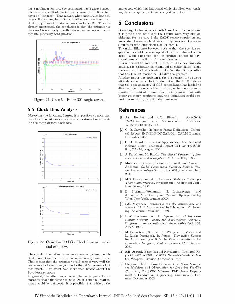
has a nonlinear feature, the estimation has a great suscep-tibility to the attitude variations because of the linearizednature of the filter. That means, when maneuvers happen,they will act strongly on its estimation and can take it outof the requirement limits as shown in figure 21. Thus, asalready mentioned, the conclusion is that the estimator inthe case 4 is not ready to suffer strong maneuvers with suchsatellite geometry configuration.

0 50 100 150 200 250 300−2.5

−2

−1.5

−1

−0.5

0

0.5

1

1.5

2

Time (s)

Eu

ler

321

erro

r (d

g)

Euler 321 angles error


Figure 21: Case 5 - Euler-321 angle errors.

5.5 Clock Bias Analysis

Observing the following figures, it is possible to note thatthe clock bias estimation was well conditioned in estimat-ing the ramp-drifted clock bias.

0 50 100 150 200 250 300

−2

−1

0

1

2

3

4

5

6

7

x 10−8

Time (s)

clo

ck b

ias

erro

r (s

)

Clock Bias error

Clock bias(s)

0 50 100 150 200 250 300

−3

−2

−1

0

1

2

3

4

5

6

7

x 10−8

Time (s)

sigm

a−cb

(s)

Standard deviation − Clock Bias

sigma−Clock bias(s)

Figure 22: Case 4 + EADS - Clock bias est. errorand std. dev.

The standard deviation convergence was very strong, whileat the same time the error has achieved a very small value.That means that the estimator could correct very well thedeviations in Pseudoranges due to the GPS receiver clockbias effect. This effect was mentioned before about thePseudorange errors.In general, the filter has achieved the convergence for allstates at about the time t = 200s. At this time all require-ments could be achieved. It is possible that, without the

maneuver, which has happened while the filter was reach-ing the convergence, this value might be better.

6 Conclusions

Observing the behavior for both Case 4 and 5 simulations,it is possible to note that the results were very similar,although for the case 5 the EADS sensor simulation hasassociated biases while it was simply unbiased Gaussiansimulation with only clock bias for case 4.The main difference between both is that the position re-quirements could be accomplished in the unbiased simu-lation, while the errors for the vertical component havestayed around the limit of the requirement.It is important to note that, except for the clock bias esti-mation, the estimator has estimated no other biases. Thus,the natural conclusion leads to the fact that it is possiblethat the bias estimation could solve the problem.Another important problem is the big sensibility to strongattitude maneuvers. In this simulation the GDOP showsthat the poor geometry of GPS constellation has leaded todisadvantage in one specific direction, which became moresensitive to attitude maneuvers. It is possible that withbetter geometry configurations, the estimation could sup-port the sensibility to attitude maneuvers.

References

[1] J.S. Bendat and A.G. Piersol. RANDOM

DATA:Analysis and Measurement Procedures.Wiley-Interscience, 1971.

[2] G. B. Carvalho. Reference Frame Definitions. Techni-cal Report INT-GEN-DF-ZAR-001, ZARM Bremen,November 2003.

[3] G. B. Carvalho. Practical Approaches of the ExtendedKalman Filter. Technical Report INT-KF-TN-ZAR-001, ZARM, August 2004.

[4] J. Farrel and M. Barth. The Global Positioning Sys-

tem and Inertial Navigation. McGraw-Hill, 1998.

[5] Mohinder S. Grewal, Lawrence R. Weill, and Angus P.Andrews. Global Positioning Systems, Inertial Nav-

igation and Integration. John Wiley & Sons, Inc.,2001.

[6] M.S. Grewal and A.P. Andrews. Kalman Filtering -

Theory and Practice. Prentice Hall, Englewood Cliffs,New Jersey, 1993.

[7] B. Hofmann-Wellenhof, H. Lichtenegger, andJ. Collins. GPS Theory and Practice. Springer-VerlagWien New York, August 2000.

[8] P.S. Maybeck. Stochastic models, estimation, and

control Vol. 1. Mathematics in Science and Engineer-ing. Academic Press Inc., 1979.

[9] B.W. Parkinson and J.J. Spilker Jr. Global Posi-

tioning System: Theory and Applications Volume I.Progress in Astronautics and Aeronautics, Vol. 163.AIAA, 1996.

[10] M. Schlotterer, S. Theil, M. Wiegand, S. Voegt, andL. Lubke-Ossenbeck, B. Peters. Navigation Systemfor Auto-Landing of RLV. In 52nd International As-

tronautical Congress, Toulouse, France. IAF, October2001.

[11] S.H. Stovall. Basic Inertial Navigation. Technical Re-port NAWCWPNS TM 8128, Naval-Air Warfare Cen-ter/Weapons Division, September 1997.

[12] Stephan Theil. Satellite and Test Mass Dynam-

ics Modeling and Observation for Drag-free Satellite

Control of the STEP Mission. PhD thesis, Depart-ment of Production Engineering, University of Bre-men, December 2002.


Documents

G. Baldo Carvalho S. Theil - dem.inpe.brhkk/2004/Gustavo-SBEIN-Paper.pdf · INTEGRATION MODEL COMPARISON FOR COUPLED NAVIGATION USING AN IMU AND THE GPS THROUGH THE EKF G. Baldo Carvalho