Funding Long Shots

Funding Long Shots*

John Hull†, Andrew W. Lo‡, Roger M. Stein§

This Draft: 24 October 2017

Abstract

We define long shots as investment projects with four features: (1) low probabilities of success; (2) long gestation lags before any cash flows are realized; (3) large required up-front investments; and (4) very large payoffs (relative to initial investment) in the unlikely event of success. Funding long shots is becoming increasingly difficult—even for high-risk investment vehicles like hedge funds and venture funds—despite the fact that some of society’s biggest challenges such as cancer, Alzheimer’s disease, global warming, and fossil-fuel depletion depend critically on the ability to undertake such investments. We investigate the possibility of improving financing for long shots by pooling them into a single portfolio that can be financed via securitized debt, and examine the conditions under which such funding mechanisms are likely to be effective.

Keywords: Capital Budgeting; Impact Investing; Venture Capital; Private Equity; Megafund; Securitization; Portfolio Theory; Research-Backed Obligation

JEL Codes: G31, G32, G24, G11

*We thank Jayna Cummings for editorial assistance. Research support from the MIT Laboratory for Financial Engineering and the University of Toronto is gratefully acknowledged. The views and opinions expressed in this article are those of the authors only, and do not necessarily represent the views and opinions of any institution or agency, any of their affiliates or employees, or any of the individuals acknowledged above. †Maple Financial Chair in Derivatives and Risk Management, Joseph L. Rotman School of Management University of Toronto, 105 St George Street, Toronto, Ontario Canada M5S 3E6. ‡Charles E. and Susan T. Harris Professor, MIT Sloan School of Management, 100 Main Street, E62–618, Cambridge, MA 02142. §Research Affiliate, MIT Laboratory for Financial Engineering, One Broadway, Cambridge, MA 02142 and Adjunct Professor of Finance, Stern School of Business, New York University.

Table of Contents

1 Introduction ................................................................................................................................................... 1

2 Literature Review......................................................................................................................................... 5

3 Long-Shot Investments .............................................................................................................................. 8

3.1 A Simple Example ................................................................................................................................ 8

3.2 Project Correlation ........................................................................................................................... 10

4 Securitization .............................................................................................................................................. 13

4.1 Application to Long Shots ............................................................................................................. 15

4.2 Analytics of Long-Shot Securitization ....................................................................................... 16

4.3 Example ................................................................................................................................................ 19

4.4 Funding Viability............................................................................................................................... 21

4.5 Correlation Assumptions ............................................................................................................... 25

5 Practical approaches to improving credit quality ........................................................................ 26

5.1 Structure of Securities .................................................................................................................... 26

5.2 Structure of Assets ........................................................................................................................... 28

6 Illustrative Examples ............................................................................................................................... 30

6.1 Rare Diseases ..................................................................................................................................... 30

6.2 Alzheimer’s Disease ......................................................................................................................... 35

7 Conclusions .................................................................................................................................................. 40

24 October 2017 © 2017 by Hull, Lo, and Stein Page 1 All Rights Reserved

1 Introduction

The standard approach to capital budgeting and investment decisions for risky projects

involves estimating a project’s expected incremental cash flows, choosing an appropriate

risk-adjusted discount rate, and calculating the net present value (NPV) of the project’s

cash flows. This approach is appropriate for many of the investment opportunities

encountered in practice, such as the replacement of plant and equipment or the

development of new products and services. We will refer to these as “textbook projects.”

Usually they are expected to lead to some level of positive future cash inflows in many

states of the world, and the key issue is to determine whether these positive inflows will be

sufficient to justify the initial investment when averaged across all possible states of the

world. In well-functioning capital markets, a textbook project can be funded if it has

positive expected NPV.

In this paper, we focus on a different type of project, which we call a “long shot.” We define

a long-shot investment as one with four specific characteristics: (1) it requires a large

amount of initial capital; (2) it has a long gestation lag, during which no cash flows are

generated and/or additional capital investment is required; (3) it has a low probability of

success; and (4) if successful, its payoff is very large relative to the initial investment.

Examples of long shots include drug development, alternative energy (fusion, wind, solar)

technology, quantum computing, commercial space travel, and mitigating the

environmental impact of climate change through geo-engineering.1

The characteristics of long shots make them much more difficult to fund on a stand-alone

basis than textbook projects. Traditionally, venture capital (VC) or philanthropic donations

have been the primary sources of funding. However, some of society’s biggest challenges

such as cancer, Alzheimer’s disease, global warming, and fossil-fuel depletion depend

critically on the ability to undertake long shots, and because of the risk profile of a typical

long shot, the funding requirements far outstrip the capital available from these traditional

sources.

1 See for example Fernandez, Stein, and Lo (2012) and Gaddy, Sivaram, and O’Sullivan (2016).


The simplest long shot is one in which there is a single up-front capital investment, a

known project duration, and a known payoff at the end of the life if the project is successful.

Suppose, for example, that a research and development (R&D) project requires an initial

investment of $200 million, lasts 10 years, and has a 5% probability of a payoff of $10

billion, and that the project’s risk is purely idiosyncratic (i.e., no priced-factor exposure). If

the discount rate for the expected cash flows from this long shot is less than 9.60%, the

project has a positive expected NPV. In principle, such a project should be quite attractive

to investors, especially given the idiosyncratic nature of the risk and current level of

interest rates.2 However, such projects are, in fact, unlikely to appeal to traditional

investors because of their scale, duration, and low probability of success, relative to their

level of expected return.

A long shot’s risk can be mitigated by forming a portfolio of many such projects. If, for

example, a “megafund” of 150 statistically independent projects—each identical to the one

just considered—were formed, the probability of at least one success would be 99.95% and

the probability of at least four successes would be about 95%. While risk has been greatly

reduced—to the point that many institutional investors would now find the investment

attractive—such a portfolio would have a 10-year duration and require $30 billion of

funding. As a result, a portfolio of such scale would be virtually impossible for any single

venture capitalist to fund.3

In this paper, we ask whether diversification and securitization techniques can be used to

structure portfolios of long shots so as to make their risk/reward profile more attractive to

a broad range of conventional institutional investors. If so, such techniques could

dramatically increase the pool of available capital to fund long shots, many of which have

social value far beyond their private-sector returns. Our secondary goal is to distinguish

projects that can be handled by the private sector from those that must, at least in the early

stages, rely on some type of government support. Although long shots may not exhibit

2 The nature of much of R&D is such that the systematic risk associated with success or failure is very low. However, there may be some systematic risk associated with the value of the project in the event of success. 3 According to the National Venture Capital Association 2017 Yearbook, the total assets under management in the U.S. VC industry in 2016 were $333.5 billion.


“market failures” in the traditional economic sense, i.e., externalities or public-goods

aspects, we propose a new kind of market imperfection: the combination of outsized scale

of investment needed to achieve acceptable levels of diversification and their high levels of

risk, which make such investments difficult to undertake using current investment vehicles.

Securitization is a particularly effective tool in dealing with scale and risk.4 Just as a

traditional asset-backed security (ABS) is used to segment the risks in a portfolio of loans

or credit default swaps to appeal to a broader range of investors, a “research-backed

obligation” (RBO) can be structured as a series of debt and equity tranches to distribute the

risks in a portfolio of long-shot R&D projects. For example, in a simple RBO structure

consisting of just three tranches—a senior tranche, a mezzanine tranche, and an equity

tranche—structured under a strict priority arrangement, the cash flows from successful

projects would flow first to the senior tranche until it has received its specified principal

and interest payments. If there were sufficient cash flows remaining, these would then flow

to the mezzanine tranche until it has received its specified principal and interest payments.

Residual cash flows would then be allocated to the equity tranche.

The advantage of a securitization structure is that it has to the potential to attract a broad

range of investors, thereby increasing the potential scale of overall funding. In our simple

example of 150 projects, the senior tranche might be rated AAA and the mezzanine tranche

BBB. The probability of default on a loan in a traditional ABS plays the same role as the

probability that a long-shot project will fail. Of course, the probability of long-shot failure

(95% in our example) is generally much higher than the probability of loss on a loan, but

the simplest RBO structure is otherwise similar to a conventional ABS in most respects.

The analogy to an ABS also highlights the important role of pairwise correlations among

projects. Our illustrative example above assumed that project successes are independent

events, but this is not usually the case. “Success correlation”—the correlation between the

success or failure of two long shots—is one of the critical factors in determining whether

private-sector funding is feasible, as in the case of traditional ABS such as mortgage-backed

securities. There are a number of reasons for positive success correlation in long-shot 4 See Fernandez, Stein, and Lo (2012).


projects. For example, the successes of cancer therapies being pursued by different teams

using the same biological pathway are related because they depend on the therapeutic

viability of that single pathway. However, unlike mortgage defaults—which became highly

correlated during the national decline in home prices starting in 20065—success

correlations among biomedical projects are unlikely to change over time in response to

market cycles.

In Section 2 we review the relevant literature and in Section 3 we describe the basic

analytical framework of long shots. We then consider the application of securitization in

Section 4, and show how correlation and other parameters affect the economic viability of

long-shot investments. More practical aspects of securitizing long-shot portfolios are

considered in Section 5, and we provide two concrete examples in Section 6, one in which

securitization is effective and one where securitization fails. We conclude in Section 7.

5 See, for example, Lo (2012).


2 Literature Review

Funding risky ventures has traditionally been the domain of the VC industry. In 2016, the

VC industry represented only $333.5 billion of the $4.5 trillion of private assets under

management in the U.S. (National Venture Capital Association (2017), Preqin (2016)), but it

has historically had a disproportionate influence on technological innovation (Kortum and

Lerner (2000)). Nevertheless, long-shot investments have remained stubbornly difficult to

fund, even through VC. Modern examples of long-shot investments can be found in the

biopharma and energy sectors, where the lack of VC funding for expansion beyond the

early-research stage is often referred to as the “Valley of Death.”

This is not a new phenomenon. The basic scale-up problem has been known for over a

century within the chemical engineering sector, where the inventor of the first synthetic

plastic, Leo Baekeland, gave the now-famous advice, “Commit your blunders on a small

scale and make your profits on a large scale” (Baekeland (1916)).

Structural explanations for the lack of funding are common. For example, the “low-

hanging fruit” or the “better than the Beatles” problem are often given as explanations for

the decline in R&D efficiency within the biopharma industry (e.g., Scannell et al. (2012)).

Rather than focusing on particular explanations for why sectors such as rare disease drug

development and clean energy technologies are different from each other (Nanda, Younge,

and Fleming (2015), Gaddy, Sivaram, and O’Sullivan (2016)), we propose to capture the

dynamics of VC funding more generally via the framework of long-shot funding processes.

An enduring characteristic of the VC industry is its high volatility (Gompers and Lerner

(2004), Kaplan and Schoar (2005)), although the degree to which this reflects

fundamentals versus investor overreaction is still under debate in some cases (Gompers et

al. (2008)). Many relate “hot” investment markets to less circumspect VC investment in

poorer quality firms, possibly through the mechanism of herding among investors

(Scharfstein and Stein (1990)). However, Robinson and Sensoy (2016) have shown that

roughly three-quarters of the underperformance of VC can be attributed to co-cyclicality of

public market valuations and net cash flows to VC funds.


Nanda and Rhodes-Kropf (2013) found that, although startups initially funded in hot

markets were more likely to go bankrupt than those funded in less active periods, hot-

market-startups that were successful had higher valuations and filed a greater number of

more highly cited patents than comparable startups funded in cold markets. In other

words, the outcomes for startups in more active markets were more likely to be in both

tails of the distribution than those funded in less active markets. This may be indicative of

heterogeneity in VC. For example, Chemmanur, Loutskina, and Tian (2014) found that

corporate VC backed a proportionately larger number of startups with better patent

outcomes than did independent venture capitalists, but that these startups were riskier and

less profitable than their counterparts. This suggests that the lack of financing of long-shot

projects may be a question of composition rather than base quality.

The institutional response of the VC community to reducing all-or-nothing risks to

investors has been to stage investments in sequential “rounds” or “raises.” At the end of

each stage, a project is abandoned, sold, or retained. Gompers (1995) showed that such

staging structures have led venture capitalists to focus primarily on early stage companies.

In some sectors, the market in intellectual property assets created by intermediate stages

acts to counter this early-stage focus, as has been the case in the biopharma industry (Gans,

Hsu, and Stern (2002)).

Gompers (1995) argues that staging is a way for venture capitalists to reduce agency costs.

Kerr, Nanda, and Rhodes-Kropf (2014) view staging as a process of experimentation that

allows both the investor and the innovator to negotiate in an environment of extreme

Knightian uncertainty. Ewens, Nanda, and Rhodes-Kropf (2015) extend this analysis to

consider how it has influenced the type of projects that are funded. They find an adaptive

shift in VC strategies toward newly viable “long-shot bets,”6 but that this shift comes at the

expense of capital-intensive projects unaffected by the innovation. Furthermore, staging

can create agency costs of its own (Cornelli and Yosha (2003), Bergemann and Hege

(2005)). For example, Nanda and Rhodes-Kropf (2014) observed that the mere possibility

6 Their usage of “long shot” is colloquial, unlike our more specific definition.


of financing risk in future stages provides a significant disincentive for investors to invest

in first-round funding for otherwise sound projects.

To bridge the so-called “Valley of Death” in biomedicine—the preclinical stages of drug

discovery through phase 2 clinical trials—Fernandez, Stein, and Lo (2012) and Fagnan et

al. (2013) proposed combining multiple long shots into a single portfolio, and then

financing that portfolio using both securitized debt and equity. Although taking “multiple

shots on goal” in drug development is expensive—requiring hundreds of millions to several

billion dollars (depending on the therapeutic area) to achieve sufficient risk reduction

through diversification—securitization allows entrepreneurs to tap into much larger pools

of capital. In 2016, the total size of U.S. debt markets was $39.4 trillion, which is

considerably larger than the VC industry’s $333.5 billion in assets under management in

that same year (of which only about $11.7 billion was invested in the life sciences.). When

one considers that, by some estimates, developing a single cancer drug can cost more than

$2 billion (DiMasi, Grabowski, and Hansen, 2016), it becomes clear that the VC community

does not have sufficient capital to provide the required funding on its own.

The present paper provides a more systematic and comprehensive analysis of the

opportunities and limitations of securitization in funding this type of project. Our analysis

is applicable to all long shots, not just those in the biomedicine area.


3 Long-Shot Investments

Consider a project which requires an initial investment I at time 0, provides a single cash

inflow at time T in the event of success, and has a T period probability of success, p. We

define the investment as a long shot if the probability of success, 𝑝, is small, its life, 𝑇, is

long (often five years or more), and the initial investment, I, is “large.” The motivation for

our definition is to capture the unique features of investment projects that have potentially

transformative payoffs, but where the required investment, risk of failure, and duration are

much higher than for typical investments. The expected cash inflow, conditional on success,

must of course be much larger than I, otherwise no rational investor would consider

investing in the project. Examples of long shots include curing cancer, generating energy

via fusion, mining asteroids and colonizing space and other planets, and geo-engineering

our planet to mitigate climate change.

We argue that it is difficult for traditional financing sources involving VC and public or

private equity to fund long shots and examine the role that can be played by securitization

instead.

3.1 A Simple Example

To see the problems in applying traditional financing structures to long shots, consider a

stylized example involving cancer drug development. Assume that the typical out-of-pocket

costs for conducting clinical trials for a single anti-cancer compound are approximately

$200 million; the average duration for these trials is 10 years; and the historical success

rate of cancer drug development programs is approximately 5%. If successful, a typical

cancer drug might generate $2 billion in annual profits for the remainder of its patent life of

10 years (a 20-year patent minus 10 years of clinical trials). Figure 1 provides a timeline of

the cash flows.


Figure 1. Timeline of revenues and costs of a hypothetical cancer drug development project.

Using a 10% cost of capital (an approximate value for the pharmaceutical industry), these

profits are equivalent to a payoff of $12.3 billion in year 10, implying an annualized

expected return from the project of 11.9%.7 However, the 95% risk of total loss is

extremely high and unlikely to interest a typical investor (especially given the 10-year

gestation lag before any cash flows can begin). Therefore, entrepreneurs have difficulty

attracting financing for such projects from traditional sources such as VC and public or

private equity.

A natural approach to solving this problem is to combine several long shots in a portfolio.

However, the low probability of success means that a large number of projects are

necessary to achieve a reasonable degree of diversification. Consider an investment in a

portfolio of 𝑛 independently and identically distributed (IID) projects similar to the one we

have just considered.8 The expected return from the portfolio is still 11.9%. Risk, as

measured by the ratio of the standard deviation of the payoff to the expected payoff, is

�1 − 𝑝𝑛𝑝

For values of n equal to 1, 10, 50, and 100 and p = 5%, this is 4.36, 1.38, 0.62, and 0.44,

respectively. As is well known, the binomial distribution approaches the normal

7 We define the “expected return” as the return provided by the expected payoff. This is the most meaningful measure as it corresponds to the maximum discount rate for which the project is attractive. Note that for a single-period long-shot project it is much greater than the expected internal rate of return. (The expected internal rate of return is −92.5% for the project considered here.). 8 In our subsequent models and simulations, we relax the IID assumption.


distribution as n increases. However, for small p, this convergence happens slowly, as is

illustrated in Figure 2 which contains the probability distribution of the number of

successes when there are 10, 50, and 100 projects.

Figure 2. Probability distribution for the number of successes when the probability of success is 0.05 and the number of projects is (a) 10, (b) 50, and (c) 100.

Unfortunately, constructing a portfolio of 100 projects similar to the one we have

considered requires $20 billion, which dwarfs the assets under management of most VCs.

Also, the risk-return profile is still not sufficiently favorable to attract VCs.

3.2 Project Correlation

In practice, project successes are rarely independent events. The Gaussian copula,

developed by Vasicek (1987) and Li (2000), is a relatively simple way of modeling success

correlation. Suppose there are n non-independent projects, each with an unconditional

probability of success equal to p. The copula model associates a standard normal

distribution with each project. Each project i is successful when the value 𝑉𝑖 obtained from

the normal distribution corresponding to the project is less than 𝑁−1(𝑝) where N is the

cumulative normal distribution function. The pairwise correlations among {𝑉𝑖} represent

the factor correlations, which, suitably transformed, result in success correlations.

0

0.05

0.1

0.15

0.2

0.25

0.3

0 1 2 3 4 5 6 7 8 9 10

(b)

0

0.1

0.2

0.3

0.4

0.5

0.6

0.7

0 1 2 3 4 5 6 7 8 9 10

(a)

00.020.040.060.08

0.10.120.140.160.18

0.2

0 1 2 3 4 5 6 7 8 9 10

(c)


The correlations between the normal distributions in the Gaussian copula model can be

generated using a factor model. In the case of a single common factor, 𝑉𝑖 (1 ≤ i ≤ n) may be

written as:

𝑉𝑖 = 𝑎𝑖𝐹 + �1 − 𝑎𝑖2𝑍𝑖 (1)

where the 𝑎𝑖 are constants (−1 ≤ 𝑎𝑖 ≤ 1) while the common factor F and idiosyncratic noise

term 𝑍𝑖 have uncorrelated standard normal distributions. The correlation between 𝑉𝑖 and

𝑉𝑗, known as the copula correlation, is then simply 𝑎𝑖𝑎𝑗. For convenience, it is often

assumed that 𝑎𝑖 equals a constant, a, for all i. Conditional on F, the successes are then

uncorrelated with probability

𝑁 �𝑁−1(𝑝) −�ρ𝐹

�1 − 𝜌�

where 𝜌 = 𝑎2 is the pairwise unconditional correlation between the Vi’s.

Discretizing the normal distribution of F, the probability, q(h), of exactly h successes from n

projects is:

𝑞(ℎ) = �𝑤𝑘𝐵(ℎ,𝑛,𝑝𝑘)𝐾

𝑘=1

(2)

where

𝑝𝑘 = 𝑁�𝑁−1(𝑝) −�𝜌𝐹𝑘

�1 − 𝜌� (3)

and 𝐵(ℎ,𝑛,𝜋) is the binomial probability that there will be h occurrences of an event in n

trials when the probability of an occurrence is 𝜋. The parameters 𝑤𝑘 and 𝐹𝑘 are the weights


and values when a standard normal distribution is approximated using Gaussian-Hermite

quadrature and K points. 9

The impact of correlation on the probability distribution of the number of defaults depends

on the number of projects and their probabilities of success. Consider the situation where

the probability of success is 10%. When there are only five projects, a copula correlation of

5% increases the standard deviation of the number of successes by only 3.5% relative to

the zero-correlation case. This is due, in part, to the observation that the distribution of

outcomes of five projects exhibits pronounced skewness, even with no correlation. With

25 and 50 projects, the distributions of outcomes are more symmetrical without

correlation, and the increase in the standard deviation is 19.5% and 36.9%, respectively.

With 100 projects (the situation in Figure 3) the standard deviation increase is 66.2%, and

with 200 projects it is over 100%.

Figure 3. Probability distribution for the number of successes in a portfolio of 100 projects when the probability of success is 0.05 and the Gaussian copula correlation is (a) 0.01, (b) 0.05, and (c) 0.10.

9 Gauss-Hermite quadrature is an accurate way of approximating the normal distribution for the purposes of numerical integration. See, for example, Davis and Rabinowitz (1975, Ch2).

0

0.02

0.04

0.06

0.08

0.1

0.12

0.14

0.16

0.18

0.2

0 1 2 3 4 5 6 7 8 9 10

(a)

0

0.02

0.04

0.06

0.08

0.1

0.12

0.14

0.16

0.18

0.2

0 1 2 3 4 5 6 7 8 9 10

(b)

0

0.02

0.04

0.06

0.08

0.1

0.12

0.14

0.16

0.18

0.2

0 1 2 3 4 5 6 7 8 9 10

(c)


The Gaussian copula model can be generalized so that more than one factor drives the

correlations. Also, other copulas with different properties can be used. One convenient

way of developing other copulas is to assume non-normal, zero-mean, unit-variance

distributions for F and 𝑍𝑖 in (1).

4 Securitization

Securitization is a well-established financing mechanism that repackages cash flows from a

portfolio of assets into securities for which there is higher investment demand.

Traditionally the assets have been debt instruments with regularly scheduled payments, so

we begin by reviewing how securitization works in this case before moving on to consider

long shots.10

Figure 4 shows a simple idealized collateralized debt obligation (CDO) in which 100 five-

year loans, each with a principal balance of $1 million and an interest rate of 5%, are

transformed into three structured securities: a senior tranche with a principal balance of

$80 million, a mezzanine tranche with a principal balance of $15 million, and an equity

tranche with a principal balance of $5 million. The tranche yields (i.e., the returns that they

will receive in the absence of any losses from defaults, assuming they are sold at par) are

3%, 7%, and 25%, respectively. The weighted average yield is 4.7%. (This is less than the

5% interest rate on the loans consistent with the creator of the structure having a positive

expected profit.) As the underlying loans are paid down, the principal and interest

payments from those loans are used to pay debt service on the senior and mezzanine

bonds, and to make equity payments.

10 See Das and Stein (2013) and Hull (2017) for a further discussion of the use of securitization and tranching for debt instruments.


Figure 4. A simple example of a five-year structure for the securitization of debt instruments. Each loan lasts five years and carries an interest rate of 5%. The weighted average yields on the tranches is 4.7%. A strict priority rule determines how cash flows are allocated to tranches. The yield indicates the return that will be realized by a tranche if no losses are allocated to the tranche. Assuming a 50% recovery rate, the equity, mezzanine, and senior tranches will earn the specified yields if the number of defaults is less than 0, 10, and 40, respectively.

We assume a simple priority rule for both principal and interest payments on the

structured securities: the senior tranche receives the first $80 million of loan principal

repayments, the mezzanine tranche receives the next $15 million, and the equity tranche

receives the last $5 million. Similarly, interim loan interest payments flow first to the senior

tranche until it has received the specified return of 3% on its outstanding principal, then to

the mezzanine tranche, and if any interest cash flows remain after the mezzanine tranche

has received its specified return of 7% on outstanding principal, they are used to provide a

return of up to 25% to the equity tranche.11

In the idealized structure in Figure 4, losses are borne first by the equity tranche. If losses

reach $5 million of par, the equity tranche is wiped out and subsequent losses are borne by

the mezzanine tranche. If losses exceed $20 million, the mezzanine tranche is also wiped

out and subsequent losses are borne by the senior tranche. Suppose that the recovery rate

11 Here we assume a simple zero-coupon structure for the senior and mezzanine tranches so that we may ignore the timing of interim interest payments.

Loan 1Loan 2Loan 3

Loan 100

Principal:$100 million

SPV

Senior Tranche (AAA)Principal: $80 million

Yield = 3%

Mezzanine Tranche (BBB)Principal: $15 million

Yield = 7%

Equity Tranche Principal: $5 million

Yield = 25%


in the event of a default on a loan is 50%. The mezzanine tranche will not lose any

principal if the number of defaults is less than or equal to 10 = $5MM/(0.5×$1M) and the

senior tranche will not lose any principal if the number of defaults is less than or equal to

40.

In practice, the rules for distributing cash flows to the tranches in a cash CDO are more

complicated than the simple structure in Figure 4. For example, there are usually more

than three tranches and some over-collateralization where the principal of the loans is

greater than the principal of tranches. In addition, there are numerous forms of credit

enhancement beyond subordination such as coverage triggers, cash flow redirection,

reserve accounts, etc. Also, there are usually some departures from the strict priority rule

we have assumed. See Section 5 for a more detailed discussion.

4.1 Application to Long Shots

The use of securitization techniques to fund biomedical innovation has been proposed by

Fernandez, Stein, and Lo (2012) and Fagnan et al. (2014). Our aim is to generalize this

approach and discuss its viability and limitations in various cases.

A portfolio of long-shot projects can be financed through the issuance of an equity tranche

and a number of debt tranches. The cash flows generated by successful projects are then

channeled to pay principal and interest on the debt tranches. When a simple strict priority

rule is used, cash inflows from successful projects go first to the senior tranche until the

cash inflows have been exhausted or the senior tranche has received its specified yield.

Excess cash inflows then go to the next-most-senior tranche until the cash inflows are

exhausted or it has received its specified yield, and so on. As in the case of a cash CDO, the

rules for allocating cash flows are usually more complicated than this (see Section 5). The

model we use here is a simplification designed to explore the key factors determining the

feasibility of securitization. Figure 5 shows a simple situation where, as in Figure 4, there

are only three tranches: a senior tranche, a mezzanine tranche, and an equity tranche. The

portfolio consists of 150 long shot projects all assumed to have identical properties. Each

project requires an investment of $200 million and has a life of five years. The probability

of a successful outcome from a project is 10% and the expected annual compound return


from a project is 10%. This means that the expected cash flow from a successful project at

the end of the five years is $3.22 billion. Given that long-shot projects typically have very

little systematic risk, the 10% expected return is attractive. (As mentioned earlier, the

systemic risk associated with R&D projects is often low.) However, it may be difficult to

obtain funding from conventional sources.

Figure 5. A simple example of a five-year structure for the securitization of long-shot projects. Each project lasts five years and requires an initial investment of $200 million. Each project has a 10% probability of success. If successful, it gives a cash flow of $3.22 billion in five years. If unsuccessful, it gives rise to no cash flows. The expected cash inflow therefore provides a return of 10%. A strict priority rule determines how cash inflows from successful projects are allocated to tranches. The yield indicates the return that will be allocated to a tranche if there are a sufficient number of project successes. The senior tranche will lose principal if there are less than six successful projects. The mezzanine tranche will lose principal if there are less than eight successful projects.

4.2 Analytics of Long-Shot Securitization

We now present analytics for securitizations similar to that in Figure 5. We assume that a

portfolio of n projects is financed by m debt tranches and an equity tranche. We denote the

probability that h of the n projects are successful by q(h). (This could be determined using

the copula model in Section 3.2, or in some other way.) We assume a simple priority rule, as

in Figure 5, and denote by 𝐾𝑗 (1 ≤ j ≤ m) the cash flow necessary to provide the first j

tranches with their promised returns. (In the example in Figure 5, m = 2, 𝐾1 = $15×1.035 =

$17.39 billion and 𝐾2 = $17.39 + $5 × 1.075 = $24.40 billion.)

Long Shot 1 Long Shot 2

Long Shot 150

Total Investment:$30 billion

SPV

Senior Tranche$15 billionYield=3%

Mezzanine Tranche$5 billionYield=7%

Equity Tranche$10 billion

Residual Cash Flows


All projects have the same life and successful projects are assumed to give rise to identical

payoff distributions at maturity. We will denote the mean and standard deviation of the

payoff from a successful project by 𝜇 and 𝜎, respectively. The coefficient of correlation

between the payoffs from each pair of successful projects will be assumed to be the same

and will be denoted by 𝜌𝑐 .

Conditional on h successful projects, the mean and standard deviation of the total payoff

available for servicing the tranches are

𝜇ℎ = ℎ𝜇

and

𝜎ℎ = 𝜎�ℎ + 𝜌𝑐ℎ(ℎ − 1)

respectively.

The simplest assumption would be that the payoffs from successful projects are

multivariate normal, implying that the total payoff from h successes is normally

distributed. However, because this assumption has the undesirable property that payoffs

from successful projects can be negative, we instead assume that the payoffs from

successful projects are lognormal, which appears consistent with empirical observations12.

The risk of a debt tranche is then given by Proposition 1 (all proofs are provided in the

Appendix):

Proposition 1: If the payoff from a successful project is lognormally distributed, the

probability, 𝜋𝑗 , that the jth tranche will receive its promised return can be

approximated as

𝜋𝑗 = �𝑞(ℎ)𝑁�ln�𝜇ℎ 𝐾𝑗⁄ � − 𝑠ℎ2 2⁄

𝑠ℎ�

𝑛

ℎ=1

(4)

12 See Fernandez, Stein, and Lo (2012) for a discussion.


where

𝑠ℎ = �ln�1 +𝜎ℎ2

𝜇ℎ2� .

The risk of the equity tranche can be approximated in a similar manner, as described in

Proposition 2:

Proposition 2: When the payoff from a successful project is lognormally distributed, the first

two moments of the payoff from the equity tranche can be approximated as

𝑀1 = �𝑞(ℎ) �𝜇ℎ𝑁 �ln(𝜇ℎ 𝐾𝑚⁄ ) + 𝑠ℎ2 2⁄

𝑠ℎ� − 𝐾𝑚𝑁 �

ln(𝜇ℎ 𝐾𝑚⁄ ) − 𝑠ℎ2 2⁄𝑠ℎ

��𝑛

ℎ=1

𝑀2 = �𝑞(ℎ)[(𝜇ℎ2 + 𝜎ℎ2)]𝑁�ln(𝜇ℎ 𝐾𝑚⁄ ) + 3 𝑠ℎ2 2⁄

𝑠ℎ�

𝑛

ℎ=1

+ 𝐾𝑚2𝑁 �ln(𝜇ℎ 𝐾𝑚⁄ ) − 𝑠ℎ2 2⁄

𝑠ℎ�

− 2𝐾𝑚 𝜇ℎ𝑁 �ln(𝜇ℎ 𝐾𝑚⁄ ) + 𝑠ℎ2 2⁄

𝑠ℎ�

where


𝜇ℎ2� .

Define the mean and standard deviation of the return (not annualized) to the equity

tranche over the life of the project as 𝜇𝐸 and 𝜎𝐸 , respectively. If E is the investment in the

equity tranche, these are related to the moments in Proposition 2 by

𝜇𝐸 =𝑀1

𝐸− 1 (5)


𝜎𝐸 =�𝑀2 −𝑀1

2

𝐸 (6)

A special case of the results in Propositions 1 and 2 is when the payoff from a successful

project is assumed to be known with certainty. By letting 𝑠ℎ tend to zero, we see that the

probability that the jth tranche receives its promised return in Proposition 1 reduces to

𝜋𝑗 = � 𝑞(ℎ)ℎ�𝜇ℎ>𝐾𝑗�

(7)

The moments of the payoff to the equity tranche in Proposition 2 reduce to:

𝑀1 = � 𝑞(ℎ)ℎ�𝜇ℎ>𝐾𝑗�

(𝜇ℎ − 𝐾𝑚)

𝑀2 = � 𝑞(ℎ)ℎ�𝜇ℎ>𝐾𝑗�

(𝜇ℎ2 + 𝐾𝑚2 − 2𝐾𝑚𝜇ℎ)

4.3 Example

We now use the analytics in Section 4.2 to explore the properties of the securitization in

Figure 5. As already noted in the structure shown in Figure 5, 𝐾1= $17.39 billion and 𝐾2 =

$24.40 billion. Also, 𝜇 = $3.22 billion. In a typical securitization of this type, the objective is

to arrange for the senior tranche to have a high investment-grade rating (e.g., AAA) and for

the mezzanine tranche to have a mid-investment-grade rating (e.g., BBB). When evaluating

tranches, credit rating agencies compare the loss forecasted by their models with the

historical loss experience on bonds and other benchmarks. Standard & Poor’s (S&P) and

Fitch use probability of default as the metric of interest when doing this analysis, while

Moody’s uses expected loss. For simplicity, we will follow the approach adopted by S&P

and Fitch in what follows. Accordingly, if the loss probability corresponds to that of a AAA

bond, the tranche is a candidate for a AAA rating. Similarly, if the loss probability


corresponds to that of a BBB bond, the tranche is a candidate for a BBB rating. Based on

statistics provided by rating agencies, we assume in what follows that the five-year default

probability must be less than 0.2% for a AAA tranche and less than 1.8% for a BBB tranche.

Consider first the case where the payoff from a successful project is known (= $3.22

billion). From (7):

𝜋1 = �𝑞(ℎ) ℎ≥6

𝜋2 = �𝑞(ℎ) ℎ≥8

If there is no success correlation, the q(h) are binomial probabilities so that 𝜋1 = 0.9981

and 𝜋2 = 0.9860. The default probabilities on the senior and mezzanine tranches are

therefore 0.19% and 1.40%, respectively. Quantitatively, this would justify considering

AAA and BBB credit ratings, respectively. However, when the success correlation is

modeled using (1)–(3) with a copula correlation of 5%, 𝜋1 = 0.9444 and 𝜋2 = 0.8724. The

senior and mezzanine tranches are then no longer close to being candidates for AAA and

BBB ratings. To increase the credit quality of the structured securities created from this

portfolio it would be necessary to either change the capital structure of the securitization

(e.g., by increasing the subordination levels) or add structural features (such as those

described in Section 5), or both.

When the payoff from a successful project is uncertain, but correlation is zero, the senior

and mezzanine tranches become slightly more risky, but the impact of this is much less

than the impact of success correlation. For example, when there is no success correlation

and no payoff correlation, increasing the standard deviation of the payoff from a success

from 0% (of the expected payoff) to 25% only increases the default probability for the

senior tranche from 0.19% to 0.22% and increases the default probability for the

mezzanine tranche from 1.40% to 1.78%. Similar results hold for the situation where the

success correlation is non-zero.


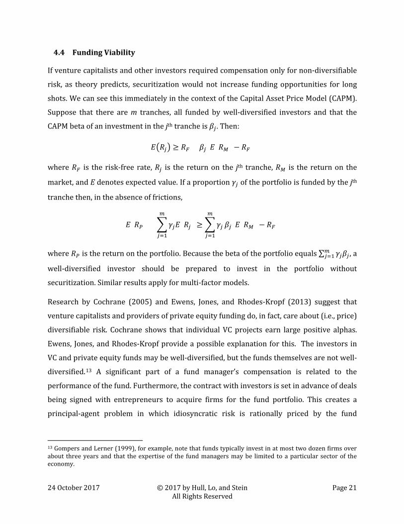
4.4 Funding Viability

If venture capitalists and other investors required compensation only for non-diversifiable

risk, as theory predicts, securitization would not increase funding opportunities for long

shots. We can see this immediately in the context of the Capital Asset Price Model (CAPM).

Suppose that there are m tranches, all funded by well-diversified investors and that the

CAPM beta of an investment in the jth tranche is 𝛽𝑗 . Then:

𝐸�𝑅𝑗� ≥ 𝑅𝐹 + 𝛽𝑗(𝐸(𝑅𝑀) − 𝑅𝐹)

where 𝑅𝐹 is the risk-free rate, 𝑅𝑗 is the return on the jth tranche, 𝑅𝑀 is the return on the

market, and E denotes expected value. If a proportion 𝛾𝑗 of the portfolio is funded by the jth

tranche then, in the absence of frictions,

𝐸(𝑅𝑃) = �𝛾𝑗𝐸(𝑅𝑗) ≥�𝛾𝑗

𝑚

𝑗=1

𝑚

𝑗=1

𝛽𝑗(𝐸(𝑅𝑀) − 𝑅𝐹)

where 𝑅𝑃 is the return on the portfolio. Because the beta of the portfolio equals ∑ 𝛾𝑗𝛽𝑗𝑚𝑗=1 , a

well-diversified investor should be prepared to invest in the portfolio without

securitization. Similar results apply for multi-factor models.

Research by Cochrane (2005) and Ewens, Jones, and Rhodes-Kropf (2013) suggest that

venture capitalists and providers of private equity funding do, in fact, care about (i.e., price)

diversifiable risk. Cochrane shows that individual VC projects earn large positive alphas.

Ewens, Jones, and Rhodes-Kropf provide a possible explanation for this. The investors in

VC and private equity funds may be well-diversified, but the funds themselves are not well-

diversified.13 A significant part of a fund manager’s compensation is related to the

performance of the fund. Furthermore, the contract with investors is set in advance of deals

being signed with entrepreneurs to acquire firms for the fund portfolio. This creates a

principal-agent problem in which idiosyncratic risk is rationally priced by the fund

13 Gompers and Lerner (1999), for example, note that funds typically invest in at most two dozen firms over about three years and that the expertise of the fund managers may be limited to a particular sector of the economy.


manager even though it would not be priced by the fund’s investors if they were

negotiating terms directly with entrepreneurs.

To assess the viability of a securitization similar to that in Figure 5, we estimate the Sharpe

ratio for the equity tranche assuming that the more senior debt tranches have been made

as large as their desired credit ratings will allow. The Sharpe ratio is the excess expected

return above the risk-free rate divided by the return standard deviation. It is a measure of

an investment’s risk/reward profile that is widely used by venture capitalists, private

equity fund managers, and hedge fund managers. As a reference point, the average Sharpe

ratio for the CRSP value-weighted return between 1970 and 2016 (calculated using a 60-

month rolling window) was 0.37 and the average realized return during this period was

10.9%.

Define 𝜋�𝑗 as the maximum probability of default for debt tranche j that is consistent with its

rating. From Proposition 1, the maximum value of Kj , 𝐾�𝑗 , is given by solving

𝜋�𝑗 = ∑ 𝑞(ℎ)𝑁 �ln�𝜇ℎ 𝐾�𝑗⁄ �−𝑠ℎ

2 2⁄

𝑠ℎ�𝑛

ℎ=1 .

The maximum size of the first tranche is 𝐾�1 and the maximum size of the jth tranche (j >1),

conditional on the sizes of earlier tranches being maximized, is 𝐾�𝑗 − 𝐾�𝑗−1.

Assume that the minimum proportion of funding to be provided by the equity tranche is e

(0 ≤ e <1). Suppose there are m debt tranches, T is the life of the projects, 𝑟𝑗 is the yield on

the jth most senior debt tranche, and C is the total funding required. The maximum

proportion of the funding that can be provided by the first (most senior) tranche is

𝑢1 = min � 𝐾�1𝐶(1+𝑟1)𝑇 , 1 − 𝑒�.

The maximum proportion of the funding that can be provided by the jth debt tranche (2 ≤ j≤

m) is

𝑢𝑗 = min�𝐾�𝑗−𝐾�𝑗−1𝐶�1+𝑟𝑗�

𝑇 , 1 − 𝑒 − ∑ 𝑢𝑘𝑗−1𝑘=1 �.


This leaves the size of the equity tranche to be 1 − ∑ 𝑢𝑗𝑚𝑗=1 .

There are a number of alternative ways of calculating the Sharpe ratio from the mean and

standard deviation of multi-year returns. We choose to define it as arithmetic average

return per year minus the risk-free rate divided by the standard deviation of the return per

year. For this purpose we assume that returns in successive years are independent. This

means that

Sharpe Ratio = 𝜇𝐸 𝑇 − 𝑟𝐹⁄𝜎𝐸 √𝑇⁄

where, as before, 𝑟𝐹 is the risk-free rate per year, and 𝜇𝐸 and 𝜎𝐸are the mean and standard

deviation of the cumulative return over the life of the structure which can be calculated

using (5) and (6) and the results in Proposition 2.

Table 1 contains results for the case in which m = 2, 𝑟1 = 3%, 𝑟2 = 7%, and T = 5, which are

the parameters corresponding to Figure 5. The risk-free rate, 𝑟𝐹, is assumed to be 2% and

we set e = 5%.14 In the top panel of Table 1, the projects are assumed to be uncorrelated

while in the bottom panel, the Gaussian copula correlation is assumed to be 5%. Figure 3b

illustrates the effect of this amount of correlation on the probability distribution of the

number of successes when there are 100 projects and the success probability is 5%.

14 Setting e > 0 ensures that there is always an equity tranche and that a Sharpe ratio for it can always be calculated.


Table 1. Minimum size, expected returns (E[Re]), and Sharpe ratios (SRe) of the equity tranche. Various combinations of the number of projects, the probability of success, the expected return, and copula correlation of projects in Figure 5 are considered. Projects are assumed to last five years. The probability of loss on the senior and mezzanine tranches are less than 0.2% and 1.8%, respectively, over the five years. Tranche yields are as in Figure 5. The risk-free rate is assumed to be 2%.

50 100 150 200 300 400

Min Size 100.00% 77.03% 66.17% 49.25% 30.73% 26.00%5% E[Re] 10.00% 10.87% 12.30% 14.48% 19.68% 22.80%

SRe 0.23 0.28 0.35 0.39 0.46 0.56Min Size 77.03% 46.84% 29.12% 20.26% 10.60% 5.16%

10% 10% E[Re] 10.86% 15.62% 20.96% 26.13% 38.44% 56.49%SRe 0.29 0.42 0.50 0.56 0.69 0.80

Min Size 50.86% 29.12% 16.77% 10.60% 5.00% 5.00%15% E[Re] 13.79% 20.95% 29.48% 38.42% 57.79% 58.71%

SRe 0.34 0.51 0.62 0.71 0.88 1.05Min Size 100.00% 64.52% 47.73% 21.59% 5.00% 5.00%

5% E[Re] 20.00% 25.31% 30.79% 47.28% 92.79% 94.37%SRe 0.40 0.53 0.66 0.74 0.92 1.10

Min Size 64.52% 17.87% 5.00% 5.00% 5.00% 5.00%20% 10% E[Re] 25.31% 52.95% 93.77% 94.37% 94.37% 94.37%

SRe 0.55 0.78 0.97 1.13 1.38 1.60Min Size 24.07% 5.00% 5.00% 5.00% 5.00% 5.00%

15% E[Re] 44.16% 93.77% 94.37% 94.37% 94.37% 94.37%SRe 0.67 0.99 1.23 1.42 1.74 2.01

Min Size 100.00% 100.00% 84.69% 77.03% 75.43% 74.62%5% E[Re] 10.00% 10.00% 10.54% 10.89% 11.34% 11.56%

SRe 0.18 0.22 0.22 0.22 0.24 0.25Min Size 100.00% 77.03% 67.77% 67.68% 61.54% 58.46%

10% 10% E[Re] 10.00% 10.87% 11.80% 12.31% 12.91% 13.25%SRe 0.24 0.25 0.26 0.28 0.29 0.29

Min Size 84.69% 66.17% 59.99% 56.90% 53.82% 52.27%15% E[Re] 10.52% 12.32% 13.12% 13.58% 14.07% 14.34%

SRe 0.27 0.30 0.31 0.32 0.33 0.33Min Size 100.00% 100.00% 76.34% 64.52% 62.04% 60.79%

5% E[Re] 20.00% 20.00% 23.12% 25.34% 26.30% 26.80%SRe 0.32 0.39 0.40 0.41 0.44 0.45

Min Size 100.00% 64.52% 50.21% 50.06% 40.57% 35.83%20% 10% E[Re] 20.00% 25.31% 29.50% 30.13% 33.88% 36.26%

SRe 0.43 0.46 0.49 0.52 0.54 0.54Min Size 76.34% 47.73% 38.19% 33.42% 28.65% 26.26%

15% E[Re] 23.10% 30.80% 35.07% 37.82% 41.17% 43.15%SRe 0.49 0.55 0.58 0.60 0.62 0.63

Number of ProjectsEquity Tranche

Success Prob

Project E[R]

0% Pairwise Correlation Among Projects

5% Pairwise Correlation Among Projects


The attractiveness of a securitization structure increases as the percentage of funding

provided by equity declines, as the expected return on the equity tranche increases, and as

the Sharpe ratio increases. Consider first the most challenging situation where the expected

return is 10% and the success probability is 5%. If projects are uncorrelated, roughly 50%

of a megafund of 200 projects could be financed by AAA and BBB bonds. This percentage

increases as the number of projects in the fund increases, but the total amount of equity

funding per project would not change substantially. The expected returns and Sharpe ratios

are not unreasonable when compared with those for the CRSP value-weighted index

mentioned earlier. However, when correlation between the projects is introduced, all

aspects of the structure become much less attractive.

As shown in Table 1, as the probability of success increases, the size of a feasible megafund

decreases and the structure becomes more attractive. For example when the success

probability is 10% (the situation in Figure 5), 150 projects would create an attractive

structure where about only 30% has to be funded from equity (so that 70% can be funded

from AAA and BBB bonds). However, the bottom panel of Table 1 indicates that the success

probability must be more than 15% when the copula correlation is 5% for such high levels

of leverage.

Increasing the expected return from 10% to 20% leads to attractive structures in the cases

of both 0% and 5% correlation. We conclude that this form of very simple securitization is

a potentially useful tool in all situations except those where the probability of success is

low and there is material correlation between the successes of different project outcomes.

4.5 Correlation Assumptions

In some situations, projects can be stratified into a small number of groups (e.g., different

broad disease categories or different sources of energy). In such cases, we expect the

within-group pairwise correlations to be greater than the between-group correlations. This

is equivalent to assuming a multi-factor model for the latent variables, 𝑉𝑖, in (1). We find

that similar results are obtained by replacing all correlations by the average correlation

(i.e., all off-diagonal entries in the correlation matrix are replaced by the average of the off-


diagonal entries). This corresponds to the assumption that is commonly made when debt

securitizations are analyzed.

5 Practical Approaches to Improving Credit Quality

The securitization model of Section 4 illustrates the relative importance of different

parameters in a long-shot securitization, but is a simplification in several respects. It

assumes that (a) all projects are entered into at the same time and have the same known

life; (b) all the funding is provided at the beginning of a project’s life; (c) a project is

categorized as a success or failure only at the end of its life; (d) a success is monetized only

at the end of a project’s life; (e) costs are known in advance; and (f) failures are written off

entirely. We have also assumed a simple zero-coupon structure for the structured debt and

that there were no structural enhancements beyond subordination.

In practice, structured transactions often depart from the assumptions of our stylized

models along two broad dimensions: the structure of the securities issued by an RBO, and

the structure and evolution of the assets in the portfolio and the markets in which they are

bought and sold.

5.1 Structure of Securities

Departures from the idealized structure of the securities primarily relate to the events on

which the security payouts depend or the mechanisms that are used to protect one or more

classes of investor.

Cash-flow securitizations are typically more complicated than the stylized structure in

Section 4 because they distribute interim, as well as final, cash flows from a portfolio of

underlying assets to investors. For example, a collateralized loan obligation (CLO) is a

simple example of a cash-flow securitization where interest and principal payments from a

portfolio of individual loans are used to repay principal and interest on tranches.

The strict priority rule we assumed in Section 4 typically applies to synthetic

securitizations (such as synthetic CDOs), but not to cash flow securitizations. In the latter,

the rules for determining how cash flows are directed to tranches can be quite complicated.


For example, cash flows are often redirected from junior to senior tranches if there is

insufficient cash flow to pay all tranches and amortization schedules may be accelerated in

such cases. This provides additional protection for senior tranches. However, it creates

path dependence and means that analytic models such as those in Section 4 serve only as

approximations. A more complete valuation generally requires a multi-period Monte Carlo

simulation model.

Some of the additional credit protection mechanisms available to cash-flow securitizations

include: reserve accounts that are pre-funded and then maintained at specific levels in

expectation of future interest and principal payments or project funding needs; coverage

triggers that require assets to be sold if specific reserves are not currently available to

cover future debt payments; and accelerated waterfalls that require the portfolio to be

prematurely liquidated to retire the bonds if certain financial criteria are not met. In

addition, the terms of the debt itself may be heterogeneous, with different amortization and

maturity schedules and periodic coupon payments, rather than a zero-coupon structure.

Table 2 summarizes some of the structural differences between the securities hypothesized

in the stylized model of Section 4 and those typically seen in the real world.

Stylized Model Real-world Securitization

Debt maturity Constant across classes Staggered by class

Coupon timing At maturity Periodic

Pre-maturity cash flows Ignored Incorporated

Structural protection Subordination Subordination, cash flow triggers, waterfall acceleration

Reserve accounts None Debt coverage, project development

Table 2. Summary of structural differences between the stylized synthetic securitization model in Section 4 and a typical long-shot securitization structure.


5.2 Structure of Assets

In our analytic models, we assume that the assets are purchased at time 0 and then

evaluated at time T, where the model time between 0 and T is considered to be a single

period. We assumed that each asset in the portfolio either realizes its exit value or fails at

time T and that there is no contingency, beyond the terminal success probability. This set of

assumptions is appropriate for synthetic transactions, but in practice cash-flow

securitizations are liable to be more complicated:

There is considerable contingency built into funding decisions and thus costs, since projects that do not pass an interim phase of advancement do not require funding for future phases (prior to reaching the exit target). Conversely, funding must also be budgeted to be available at dates beyond the initial investment.

Projects reach target exit phases at different rates. Thus, while some projects are still advancing, others may have already reached their exit target. Sales of these projects provide additional capital to fund development of remaining projects still in the portfolio. Furthermore, it is possible to exit some projects early, but still at a profit if they have advanced part-way through the development process. This is particularly helpful if additional capital is required for debt servicing. This “time tranching” also serves to reduce correlation.

Asset sales are not necessarily instantaneous (as is the case when the assets are, for example, corporate bonds). In the case of long-shot projects, buyers must be found and terms negotiated before an exit may take place. This typically takes additional time so that there is a lag between the time a portfolio manager decides to sell a project and the time that proceeds of the sale are received.

Table 3 summarizes these and other features that differentiate typical long-shot assets

from those in the stylized model of Section 4, and Figure 6 contains a schematic description

of how a cash-flow securitization with coupon-paying debt might be structured for a

portfolio of early-stage drug compounds. Not shown in Figure 6 are reserve accounts or the

various changes to the portfolio and cash-flow structure that may occur when, for example,

available funds are not sufficient to ensure that future debt payments can be made, and

therefore cash flow is redirected or assets are sold early to raise capital.


Feature of assets Stylized Analytic Model Real-world Securitization

Timing of cash flows Fixed Variable

Arrival time of transitions Fixed Variable

Monetization One time Staged

Development Costs Fixed Variable

Payment timing for costs One time up-front Multiple throughout

Contingency of costs Deterministic Contingent

Acquisition timing Instantaneous Staged

Exit timing Instantaneous Delayed

Table 3. Summary of differences in assets between the stylized securitization model in Section 4 and a typical long-shot securitization structure.

Figure 6. Schematic design of a cash-flow securitization, with coupon-paying debt, for a portfolio of early-stage drug development projects in which: (1) securities are issued; (2) proceeds from the sale of the securities are used to purchase a portfolio of candidate therapies (sometimes over a period of time); (3) as therapies move through the approval process, they gain value and are sold or they fail and are withdrawn; (4) proceeds of the sales are used to pay principal and interest and to fund trials on remaining drugs; and (5) at end of the transaction, the remaining portfolio is sold and the proceeds the distributed.


Fernandez, Stein, and Lo (2012) and Fagnan et al. (2014) have developed an open-source

library of software tools (called RBOToolbox) to simulate the performance of securitization

structures with behaviors such as those depicted in Figure 6. The simulation results for

hypothetical megafunds in oncology and in rare diseases yield attractive risk/reward

profiles when compared to current market investment opportunities. The results also

suggest that the flexibility built into real-life structures often increases the protection

provided to bondholders, allowing a greater percentage of funding to come from AAA and

BBB bonds than suggested by the simple model of Section 4. We provide a more detailed

analysis of the benefits of different components of cash flow securitization in the first

example in Section 6.

However, securitization is not a panacea. In situations where the number of distinct

research approaches is small and the projects’ success probabilities are low, securitization

is not feasible for the reasons discussed in Section 4.4. We illustrate both of these cases in

the next section.

6 Illustrative Examples

To illustrate the range of applications of long-shot financing, we provide two examples at

opposite extremes: a portfolio of rare-disease therapeutics and a portfolio of Alzheimer’s

disease (AD) therapeutics. For reasons that will become clear once we describe the

risk/reward profiles of each investment, the former can be easily financed with both

securitized debt and equity, particularly when additional securitization techniques such as

those discussed in Section 5 are used, whereas the latter is virtually impossible to finance

using any purely private-sector means.

6.1 Rare Diseases

According to the Orphan Drug Act of 1983, rare or “orphan” diseases are considered to be

those that affect fewer than 200,000 patients in the U.S. Developing successful therapies for

such diseases are long shots—the success rate, from the preclinical phase to FDA approval


ranges from less than 1% to 20% and higher, depending on the condition and type of

therapy. This is still much higher than for many other drug development areas and is due,

in part, to the scientific properties of many orphan diseases which are often caused by a

single mutation in a patient’s genome. This property results in two features that are

particularly well-suited to portfolios. First, the research on therapies may move directly to

the treatment of the mutation, rather than having to first establish the cause of the disease,

shortening development time and increasing the odds of success. Second, because many

diseases are monogenic (i.e., they are caused by a random mutation in a single gene), the

success correlations among different therapeutic programs is likely to be low. In addition

to these scientific properties, and although patient populations are often quite small, there

are additional financial considerations that make these therapies more economically

viable: they often receive faster regulatory approval (shorter trials), patients are often

registered through foundations and can thus be pre-screened and identified (leading to

smaller, cheaper trials), there are often periods of extended patent exclusivity (due to

legislative actions), and patients are readily reimbursed for treatments (leading to

attractive valuations upon success).

Following Fagnan et al. (2014) and Fagnan et al. (2015), we analyze a hypothetical

portfolio of orphan disease therapies. The goal of such a megafund is to purchase candidate

therapies at the preclinical or early phase 1 stage, where the drugs are typically very risky

and therefore difficult to fund individually, and to use the fund as a vehicle to finance trials

through to the much less risky phases 2 and 3 where investors have greater capacity given

their risk tolerance.15

We adopt most of the calibrations in Fagnan et al. (2014), including: (1) the success

probabilities, trial costs, and exit valuations; (2) the promised yields of the senior and

subordinated debt (5% and 8%, respectively); and (3) the assumption that the target

15 In order to be approved for use in patients, a drug must undergo a number of trial phases, each of which requires a larger population of test subjects and capital to fund, but the success of which increases the probability of ultimate approval and therefore increases the economic value of the compound. In the U.S., for example, the FDA mandates that phase 1 trials test the drug’s safety and dosage (typically 20-80 subjects), phase 2 trials test the drug’s efficacy and side effects (hundreds of subjects), and phase 3 trials test more rigorously the drug’s efficacy and further test dosing and adverse reactions (thousands of subjects).


portfolio consists of an equal number of preclinical compounds and phase 1 compounds

(acquired at launch), that all compounds have target exits in phase 3, and all forms of

structured exits such as deferred milestone payments, etc. are ignored. However, we

modify some assumptions related to the megafund’s capital structure:

Fagnan et al. (2014) assumed a capital structure of 15% senior debt, 20% subordinated

debt, and 65% equity. Our simulations assume 30% senior debt, 20% subordinated debt,

and 50% equity, which is somewhat more consistent with current market transactions.

To demonstrate the impact of different cash-flow structuring profiles, we

– structure debt as either coupon-paying or zero coupon; – structure maturities as either concurrent or staggered; and – include and exclude budgeting for debt service payments.

Our goal in varying the debt structure is to explore the impact that structuring can have on

the credit quality of the debt. While these results are specific to the transaction structure in

our example, they are directionally consistent with comparable results from other

structures.

The results of our simulation are given in Table 4 (a companion table in the Appendix

contains details of the structural differences between the simulations). The first rows of the

table show the probabilities of default for the senior and subordinated debt tranches (“PD

senior” and “PD subordinated,” respectively) along with the S&P rating that has the closest

historical default rate to the estimate for the debt maturity, based on S&P’s historical

default studies (Standard & Poor’s, 2016, Table 26). The next rows show the mean

annualized return on equity (ROE) for the equity holders along with the probabilities of a

loss to equity (“P(equity loss)”) and the probability of large returns (“P(ROE > 25%)”).

Finally, the last row of the table shows the average number of therapies successfully

advanced at least one phase through the approval process.


(1)

Simulation light structuring, zero coupon

(2)

Simulation light structuring, semi-annual coupon

(3)

Simulation fuller structuring, semi-annual coupon

(4)

Equity only

PD senior 9.4 % 1.2 % 7 bps -

Closest S&P historical default rate BB / BB- BBB AAA -

PD subordinated 22.1 % 4.4 % 1.7 % -

Closest S&P historical default rate B/B- BBB- / BB+ BBB+ / BBB -

ROE (mean) 15.0% 10.8% 13.8% 10.1%

P(equity loss) 17.3% 18.4% 14.5% 19.9%

P(ROE > 25%) 34.3% 23.2% 27.7% 9.9%

Mean drugs exiting (P2/P3) 2.7 / 4.3 3.6 / 3.5 2.9 / 4.2 0.9 / 2.4

Table 4. Summary of orphan disease megafund simulation with 1 million paths using debt structured as (1) zero coupon with no reserves or overcollateralization; (2) coupon paying debt with no reserves or overcollateralization; (3) coupon paying debt with reserves and overcollateralization; and (4) no debt but the same starting equity. The table shows the probabilities of default for senior and subordinated debt, the corresponding S&P ratings with the closest historical default rate, the mean annualized ROE for equity holders; probability that ROE < 0; and the probability that ROE > 0.25. It also shows the drugs exiting at phase 2 (P2) and phase 3 (P3). Portfolios contained an average of 16 (8) compounds when structured with (without) debt (see Appendix A.3).

As expected, the ROE results suggest that adding leverage generally increases the expected

return for the transaction. However, this advantage is mediated by the tradeoff between

increased purchasing power in constructing the portfolio (by virtue of a larger, levered

capital base) and the need to service debt, which reduces returns both by siphoning off

cash flow and by constraining portfolio growth (due either to the need to reduce

development costs in order to service debt, or, in some cases, to sell assets to meet debt

servicing requirements). Also, because more assets are purchased when using leverage,

levered transactions advance a larger number of projects (in this case, by advancing more

drugs through to phases 2 and 3).


A comparison of the columns of Table 4 suggests that the use of some of the structuring

elements of Section 5 appears to improve both the credit quality of the debt and the returns

to equity holders. In general, more structuring results in higher returns and lower

probabilities of default, with the probability of the simple zero-coupon structure exhibiting

a default probability more than two orders of magnitude larger than its more structured

counterpart. In addition, the risk to equity in using debt financing tends to be improved as

more structuring tools are applied, due in part to the increased diversification when a

larger number of assets is purchased. In this example, the probability of a loss to equity

decreases when a larger portfolio is financed (using debt), and the decrease is substantial

in the case of the most structured bond (see column 3): the probability of a negative return

is about 14.5%, versus 19.9% for straight equity (see column 4). It is also notable that the

probability of realizing an ROE of greater than 25% rises to 27.7% for the highly structured

transaction versus only 10% for the smaller, equity-only portfolio.

Note that the returns for the more fully structured case in Table 4 likely understate the

performance of the transaction because we assume the same coupons on debt for all of the

debt transactions, even though the more heavily structured transaction uses debt with

shorter average maturities and much lower default probabilities. It is likely that the

coupon on a zero-coupon bond with a five-year maturity and a 9.4% probability of default

would be much higher than that of a four-year maturity bond making semi-annual

payments with a default probability of just 7 basis points (bps). Such a difference in

coupons for these two bonds would magnify the differences in ROE by virtue of more cash

flow being directed to the portfolio and less to debt service. (The lower (higher) coupon

rates would also likely reduce (increase) the default probabilities for the bonds.)

This example demonstrates the importance of including real-world features in the analysis

of long-shot portfolios, but there are still more features that we have not included. For

example, given the complexities in negotiating transactions for exiting investments in

biomedical projects, it is likely that an initial portfolio would not be fully constructed at

closing and may take several years to complete. This timing is not captured by our

simulations.


More importantly, it is typical (currently about 90% of the time) for biomedical projects to

exit under terms involving a combination of an up-front payment and one or more

“milestone” payments that are subsequently paid to the seller upon the successful

achievement of additional clinical and commercial objectives by the buyer. For example, a

drug may be sold in phase 2 for $50 million up-front and another $25 million that is

payable by the buyer to the seller if the drug achieves its phase 3 endpoints. Such deal

terms have significant implications for the timing of cash flows which, in turn, affect the

default probabilities of the bonds, the correlation of cash flows, and the return to equity

holders.

6.2 Alzheimer’s Disease

An example of the limitations of long-shot financing can be seen in the case of drug

development for AD which is studied by Lo et al. (2014). Because the basic biology of AD is

less well developed than that of other diseases, formulating targets for drug development is

more difficult. Moreover, clinical trials for neurodegenerative diseases like AD often cost

more (up to $600 million vs. $200 million for a typical cancer drug and even less for a

targeted orphan disease therapy); take longer (13 years vs. 10 years in oncology), which

yields a shorter patent life upon approval; and have lower estimated probabilities of

success (see below). However, given that 5 million Americans are currently estimated to

suffer from AD, the earnings per year of an approved AD drug are considerably higher than

those of the average cancer drug (estimated at $5 billion vs. $2 billion per year), yielding an

NPV of $24.3 billion at approval.

The clearest manifestation of these combined challenges is that there have been no new AD

drugs approved by the FDA since 2003.

This is in a sharp contrast to the 36 cancer drugs approved between January 2015 and

April 2017. In fact, after informally polling a number of AD experts, Lo et al. (2014)

reported identifying only 64 potential AD targets, of which only two to three,

predominantly, were being pursued by the biopharma industry. Within the months prior to

this writing, there have been at least four highly visible failures of AD drug candidates in

phase 3 trials (Lilly’s solanezumab in November 2016, Lundbeck’s idalopirdine and


Merck’s verubecestat in February 2017, and Axovant’s intepirdine in September 2017),

raising further doubts in the minds of investors about this therapeutic area.

To examine what this implies for long-shot financing, we performed a variation of the

simulation in Lo et al. (2014). Consider a stylized megafund of 64 AD drug candidates with

the cost and revenue parameters in Table 5:

Cost per project $600 million Clinical trial duration 13 years Remaining patent life 7 years

Earnings per year $5 billion Cost of capital 10%16

Table 5. Parameters used for analysis of Alzheimer’s megafund.

The total cost of constructing the portfolio of 64 AD candidate therapies is 64 × $600

million = $38.4 billion and the NPV of the payoff for a single successful project is $24.3

billion, so that at least two successful projects are required just to recover the initial

investment (assuming no other fees or expenses). In the scenario of two successful drugs,

the investor would receive $48.6 billion in NPV, yielding a total return (not annualized) for

the 20-year investment of R = 48.638.4 − 1 = 𝑅 = 48.6

38.4 − 1 =26.6%, or just over 1% per year

annualized.

The only two remaining parameters needed to simulate the investment performance of an

AD megafund are the probability of success of each project and the pairwise correlation

among projects, if any. Because there have been no successful AD drugs developed over the

last 14 years, the probability of success is difficult to estimate. In the most recent published

study, Cummings, Morstorf, and Zhong (2014) estimate a failure rate of 99.6% for a 0.4%

16 Note that the 10% assumption for cost of capital is generous. For example, Kerins, Smith, and Smith (2004) and Moeza and Sahut (2013) both find that for diversified biotechnology venture investors, a gross cost of capital in the range of 13% to 15% is reasonable.


probability of success using a sample of 413 AD trials from 2002 to 2014.17 For simplicity,

we run simulations with p = 1%, 5%, and 10% for illustrative purposes. With respect to

pairwise correlation, we follow Lo et al. (2014) and use equicorrelated multivariate normal

latent variables to simulate correlated Bernoulli trials.18

The cumulative distribution functions (CDFs) for the total number of successes (out of 64

trials) are displayed in Figure 7 for various pairwise correlation assumptions. The red line

shows the results when using average estimated pairwise correlations provided by several

AD experts, while the interpretation of the others is given in the legends.

We also show results for the success correlation, 𝜌, ranging from 0% to 75%—Figure 7a

contains the CDFs for p = 1%, and the two remaining subfigures contain the CDFs for p =

5% and 10%. These figures show that the distribution of the total number of successes

depends heavily on 𝜌. With 𝜌 = 0% and p = 1%, the probability of at least one success out of

64 trials is 47.5%; with 𝜌 = 5%, this probability becomes 43.7%; with 𝜌 = 10%, this

probability becomes 40.2%; and with 𝜌 = 75%, this probability declines to 9.9%.

Of course, the impact of higher pairwise correlation is diminished when the probability of

success for each Bernoulli trial is higher. For example, Figure 7c shows that when p = 10%,

the probability of at least one success ranges from 99.9% with 𝜌 = 0% to 45% with 𝜌 =

75%, almost as high as in the case with p = 1% and 𝜌 = 0%. Therefore, the impact of success

correlation on default probabilities can be mitigated by selecting projects with higher

probabilities of success. However, doing so is akin to identifying investments with positive

“alpha”; it is easier said than done.

17 Using the “Rule of Threes,” the naïve 95% upper bound on the estimate of the success rate, having observed zero successes in 413 trials, would be 3/413= 0.07%. By similar calculations, a naïve 99% upper bound on the success rate would be 1.1% and a 99.9% upper bound would be 1.7% (assuming no correlation). 18 This is equivalent to the Gaussian copula model (1).


(a) (b)

(c)

Figure 7. Cumulative probability distribution functions for the number of successes, k, in 64 trials with equal pairwise correlation ranging from 0% to 75%, and correlation determined by averaging expert opinion (see Lo et al., 2014), for probability of success p equal to (a) 1%; (b) 5%; and (c) 10%. To show more detail in the left tail of the distribution functions, the graphs display only up to k = 25.

The performance results for the hypothetical AD megafund are contained in Table 6. With

𝑝 = 1% and 𝜌 = 0%, the expected annualized return is −53.4% with an annualized

standard deviation of 49.1%. And this is the best-case scenario for the fund when 𝑝 =

1%—as 𝜌 increases, the fund’s performance becomes worse, yielding an expected return of

−89.5% with 𝜌 = 75%. With such performance, no rational investor would participate in

this fund, hence securitization is not a feasible alternative.

Performance improves somewhat when 𝑝 = 5%. With no pairwise correlation, the

expected return in this case is 1% and the standard deviation is 20.3%. However, with even

the slightest positive correlation, the fund’s expected return becomes negative. Only when

the probability of success reaches 10% does megafund financing become feasible. But even

0.0%

20.0%

40.0%

60.0%

80.0%

100.0%

0 1 2 3 4 5 6 7 8 9 10 11 12 13 14 15 16 17 18 19 20 21 22 23 24 25

Correlation = 0%

Correlation = 5%

Correlation = 10%

Correlaton = 25%

Correlation = 50%

Correlation = 75%

Experts

0.0%

20.0%

40.0%

60.0%

80.0%

100.0%

0 1 2 3 4 5 6 7 8 9 10 11 12 13 14 15 16 17 18 19 20 21 22 23 24 25

Correlation = 0%

Correlation = 5%

Correlation = 10%

Correlaton = 25%

Correlation = 50%

Correlation = 75%

Experts

0.0%

20.0%

40.0%

60.0%

80.0%

100.0%

0 1 2 3 4 5 6 7 8 9 10 11 12 13 14 15 16 17 18 19 20 21 22 23 24 25

Correlation = 0%

Correlation = 5%

Correlation = 10%

Correlaton = 25%

Correlation = 50%

Correlation = 75%

Experts


in this extreme case, once pairwise correlations reach 25%, the expected return becomes

negative and megafund financing is again infeasible.

There is, of course, some level of p beyond 10% for which the expected return is positive,

but in the context of AD, such levels are currently unrealistic.

Table 6. Performance statistics of a hypothetical portfolio of 64 AD drug candidates over a 13-year investment period, each with probability of success, p, ranging from 1% to 10% and pairwise correlations, 𝝆, ranging from 0% to 75%, and with success probabilities and correlations determined by experts. E[hits]: expected hits; E[R]: expected returns; SD[R]: standard deviation.

Motivated by the results above, an alternative strategy to “picking winners” is to construct

portfolios containing many different therapeutic approaches, which can reduce correlation.

At one extreme, if all projects are perfectly correlated, the probability of one success is the

same as the probability of 64 successes. By investing in a more diverse portfolio, perhaps

containing more unconventional approaches, the portfolio’s expected returns may be

improved due to the reduction in correlation. These more unorthodox therapies may have

lower probabilities of success. However, the diversification benefit they confer could

overcome their (relatively) lower likelihood of paying off, particularly for portfolios with

such low initial probabilities of success. This technique—trading asset quality for portfolio

diversification—is routinely employed by credit portfolio managers in managing more

conventional fixed-income portfolios (Bohn and Stein, 2009). However, an important

constraint on our results is the availability of viable AD therapies in which to invest. In

p ρ E[hits]Prob at

least 1 hit E[R] SD[R] p ρ E[hits]Prob at

least 1 hit E[R] SD[R]

1% 0% 0.6 47.5% -53.4% 49.1% 10% 0% 6.4 99.9% 10.6% 5.3% 1% 5% 0.6 43.7% -56.9% 49.0% 10% 5% 6.4 98.9% 9.0% 12.4% 1% 10% 0.6 40.2% -60.2% 48.6% 10% 10% 6.4 97.2% 6.7% 19.2% 1% 25% 0.6 31.3% -68.7% 46.6% 10% 25% 6.4 88.4% -3.3% 35.7% 1% 50% 0.6 19.3% -80.2% 40.6% 10% 50% 6.4 68.4% -24.8% 51.7% 1% 75% 0.6 9.9% -89.5% 31.8% 10% 75% 6.4 45.0% -49.5% 56.4%

5% 0% 3.2 96.3% 1.0% 20.3% 3.8 78.5% -16.7% 44.0% 5% 5% 3.2 91.6% -4.0% 29.6% 5% 10% 3.2 86.7% -9.0% 36.0% 5% 25% 3.2 72.5% -23.7% 47.4% 5% 50% 3.2 50.3% -46.3% 53.7% 5% 75% 3.2 29.7% -67.4% 50.5%

Experts


practice, we are limited simply by the small number of distinct targets, mechanisms of

action, and researchers in the field.

Although AD therapies currently do not appear to be conducive to a purely private-sector

funding model, this should not be interpreted as motivation to divest from AD therapeutics

(although several large pharma companies seem to be doing just that). Instead, it

underscores the need for some sort of government intervention to address this societal

challenge. In fact, Lo et al. (2014) show that, from a public policy perspective, government

investment in an AD megafund may yield potentially highly attractive rates of return when

we include the projected cost savings to taxpayers of delaying the onset or slowing the

progression of AD (e.g., according to the Alzheimer’s Association (2017), the projected

2017 spending on AD by Medicare and Medicaid alone is $175 billion).

Additional research can lead to both improved probabilities of technical success (as the

scientific community expands its knowledge of the biology of AD) and a more diverse set of

therapeutic alternatives (as funding becomes available to finance research on novel

scientific approaches). Through more creative government-backed programs such as long-

term AD bonds backed by government guarantees (such as those described in Fagnan, et

al., 2013), these dual outcomes may serve, over time, to transform AD drug development to

a purely private-sector pursuit.

7 Conclusions

Long shots play a key role in innovation—they are the means by which some of society’s

biggest challenges will be met. In this paper, we propose the use of securitization to finance

long shots, a well-established financing technique uniquely suited because of the scale and

scope of debt markets and their risk-sharing capacity.

The viability of the securitization structure we have proposed depends critically on the

number of available projects, their probabilities of success, the costs of development, the

relative relationship between these costs and the payoff upon success, and the correlations

between projects. Because of the sensitivity of default probabilities to these correlations, it

is important to maximize diversification among the projects chosen for the portfolio. Of


course, greater diversity also means greater expertise required to manage the portfolio,

hence a balance must be struck.

We also show that in some settings, credit quality may be improved dramatically through

the use of more involved structuring techniques. While such techniques cannot turn a

negative NPV investment positive, they do permit more efficient use of the returns

generated by portfolios of positive NPV projects to service structured debt backed by the

portfolio. This may result in significant increases in the credit quality of the structured

debt, even when projects are correlated. We provide an example of such performance

improvement on portfolios composed of identical assets, but differing structures and

structural enhancements.

Finally, our analysis has the potential to allow us to distinguish projects that can only be

funded by the government from those that can be funded by the private sector. For long

shots that yield a much higher return to society than to the private sector, government

funding must be used to bridge the financing gap, perhaps in the form of public/private

partnerships. Except for these cases, however, it appears feasible to finance long shots

through private-sector securitization as described in this paper.


References

Aitchison, John and J. Alan C. Brown. 1957. The Lognormal Distribution, Cambridge, England: Cambridge University Press.

Alzheimer’s Association. 2017. 2017 Alzheimer’s Disease Facts and Figures. Chicago, IL: Alzheimer’s Association.

Baekeland, Leo H. 1916. “Practical Life as a Complement to University Education—Medal Address.” Journal of Industrial and Engineering Chemistry 8, 184-190.

Bergemann, Dirk, and Ulrich Hege. 2005. “The Financing of Innovation: Learning and Stopping.” RAND Journal of Economics 36, 719–752.

Bohn, Jeffrey and Roger M. Stein, 2009. Active Credit Portfolio Management in Practice. Upper Saddle River, New Jersey: Prentice Hall.

Chemmanur, Thomas J., Elena Loutskina and Xuan Tian. 2014. “Corporate Venture Capital, Value Creation, and Innovation.” Review of Financial Studies 27, 2434–2473.

Cochrane, John H. 2005. “The Risk and Return of Venture Capital.” Journal of Financial Economics 75, 3-52.

Cornelli, Francesca, and Oved Yosha. 2003. “Stage Financing and the Role of Convertible Securities.” Review of Economic Studies 70, 1–32.

Cummings, Jeffrey L., Travis Morstorf, and Kate Zhong. 2014. “Alzheimer’s Disease Drug Development Pipelines: Few Candidates: Frequent Failures.” Alzheimer’s Research & Therapy 6, 37.

Das, Ashish and Roger M. Stein, 2013. “Differences in Tranching Methods: Some Results and Implications,” in Credit Securitisations and Derivatives: Challenges for the Global Markets, edited by Daniel Rösch and Harald Scheule, 173–186. New York: John Wiley & Sons.

Davis, Philip J. and Philip Rabinowitz. 1975. Methods of Numerical Integration. New York: Academic Press.

DiMasi, Joseph A., Henry G. Grabowski, Ronald W. Hansen, 2016. “Innovation in the pharmaceutical industry: New estimates of R&D costs.” Journal of Health Economics 47, 20–33.

Ewens, Michael, Charler Jones, and Matthew Rhodes-Kropf, 2013. “The Price of Diversifiable Risk in Venture Capital and Private Equity.” Review of Financial Studies 26, 1853–1889.

Ewens, Michael, Ramana Nanda, and Matthew Rhodes-Kropf. 2015. “Entrepreneurship and the Cost of Experimentation.” Harvard Business School Working Paper 15-070.

Fagnan, David E., Jose-Maria Fernandez, Andrew W. Lo, and Roger M. Stein. 2013. “Can Financial Engineering Cure Cancer?” American Economic Review Papers & Proceedings 103, 406–411.


Fagnan, David E., Austin A. Gromatzky, Roger M. Stein, Jose-Maria Fernandez, and Andrew W. Lo. 2014. “Financing Drug Discovery for Orphan Diseases.” Drug Discovery Today 19, 533–538.

Fagnan, David E., N. Nora Yang, John C. McKew, and Andrew W. Lo. 2015. “Financing Translation: Analysis of the NCATS Rare-Diseases Portfolio.” Science Translational Medicine 7, 276ps3.

Fenton, Lawrence F. 1960. “The Sum of Lognormal Probability Distributions in Scatter Transmission Systems.” IRE Transactions in Communications Systems 8, 57–67.

Fernandez, Jose-Maria, Roger M. Stein, and Andrew W. Lo. 2012. “Commercializing Biomedical Research Through Securitization Techniques.” Nature Biotechnology 30, 395–400.

Gaddy, Benjamin, Varun Sivaram, and Francis O’Sullivan. 2016. “Venture Capital and Cleantech: The Wrong Model for Clean Energy Innovation.” Massachusetts Institute of Technology, MITEI-WP-2016-06.

Gans, Joshua S., David H. Hsu, and Scott Stern. 2002. “When Does Start-Up Innovation Spur the Gale of Creative Destruction?” The RAND Journal of Economics 33, 571–586.

Gompers, Paul. 1995. “Optimal Investment, Monitoring, and the Staging of Venture Capital.” Journal of Finance 50, 1461–1489.

Gompers, Paul, Anna Kovner, Josh Lerner, and David Scharfstein. 2008. “Venture capital investment cycles: The impact of public markets.” Journal of Financial Economics 87, 1–23.

Gompers, Paul, and Josh Lerner. 1999. “An analysis of compensation in the U.S. venture capital partnership.” Journal of Financial Economics 51, 3–44.

Gompers, Paul, and Josh Lerner. 2004. The Venture Capital Cycle. Cambridge, MA.: MIT Press.

Hull, John. 2017. Options, Futures and Other Derivatives, 10th edition. New York: Pearson.

Kaplan, Steven, and Antoinette Schoar. 2005. “Private Equity Performance: Returns, Persistence and Capital Flows.” Journal of Finance 60, 1791–1823.

Kerins, Frank, Janet Kiholm Smith, and Richard Smith. 2004. “Opportunity Cost of Capital for Venture Capital Investors and Entrepreneurs.” Journal of Financial and Quantitative Analysis 39, 385–405.

Kerr, William, Ramana Nanda, and Matthew Rhodes-Kropf. 2014. “Entrepreneurship as Experimentation.” Journal of Economic Perspectives 28, 25–48.

Kortum, Samuel, and Josh Lerner. 2000. “Assessing The Impact Of Venture Capital On Innovation.” RAND Journal of Economics 31, 674–92.

Li, David X. 2000. “On Default Correlation: A Copula Function Approach.” Journal of Fixed Income 9 (4), 43–54.


Lo, Andrew W. 2012. “Reading About the Financial Crisis: A Twenty-One-Book Review.” Journal of Economic Literature 50 (1), 151–178.

Lo, Andrew W., Carole Ho, Jayna Cummings, and Kenneth S. Kosik. 2014. “Parallel Discovery of Alzheimer’s Therapeutics.” Science Translational Medicine 6, 241–245.

Moeza, Khalfallah and Jean Michel Sahut. 2013. “Evaluation Cost of Venture Capital for Investors and Entrepreneurs in the French Market.” International Journal of Business 18, 81–98.

Nanda, Ramana and Matthew Rhodes-Kropf. 2013. “Investment Cycles and Startup Innovation.” Journal of Financial Economics 110, 403–418.

Nanda, Ramana, and Matthew Rhodes-Kropf. 2014. “Financing Risk and Innovation.” Harvard Business School Working Paper 11-103.

Nanda, Ramana, Ken Younge, and Lee Fleming. "Innovation and Entrepreneurship in Renewable Energy." 2015. Chap. 7 in The Changing Frontier: Rethinking Science and Innovation Policy, edited by Adam Jaffe and Benjamin Jones, 199–232. Chicago: University of Chicago Press.

National Venture Capital Association. 2017. 2016 National Venture Capital Association Yearbook. New York: Thomson Reuters.

Preqin. 2016. 2016 Preqin Global Private Equity & Venture Capital Report.

Robinson, David T., and Berk A. Sensoy. 2016. “Cyclicality, Performance Measurement, and Cash Flow Liquidity in Private Equity.” Journal of Financial Economics 122, 521–543.

Scannell, Jack W., Alex Blanckley, Helen Boldon, and Brian Warrington. 2012. “Diagnosing The Decline In Pharmaceutical R&D Efficiency.” Nature Reviews Drug Discovery 11, 191–200.

Scharfstein, David S. and Jeremy C. Stein. 1990. “Herd Behavior and Investment.” American Economic Review 80, 465–479.

Standard & Poor’s. 2016. Default, Transition, and Recovery: 2015 Annual Global Corporate Default Study and Rating Transitions. New York: Standard & Poor’s Financial Services.

Vasicek, Oldrich 1987. “Probability of Loss on a Loan Portfolio.” Working Paper, KMV.


APPENDIX A.1 Proof of Proposition 1

To prove Proposition 1 we note that the sum of variables that are multivariate lognormal is

approximately lognormally distributed. Appropriate parameters for the lognormal

distribution of the sum can be determined by moment matching.19 Define 𝑚ℎ and 𝑠ℎ as the

mean and standard deviation of the logarithm of total payoff from h successes. From the

properties of the lognormal distribution, we require

𝜇ℎ = exp(𝑚ℎ + 𝑠ℎ2 2⁄ )

𝜎ℎ2 = 𝜇ℎ2[exp(𝑠ℎ2) − 1]

so that


𝜇ℎ2�

𝑚ℎ = ln(𝜇ℎ) − 0.5𝑠ℎ2

Conditional on h successes, the probability that the payoff will be greater than 𝐾𝑗 is

𝑁�𝑚ℎ − ln �𝐾𝑗�

𝑠ℎ�

The result in Proposition 1 follows from substituting for 𝑚ℎ.

A.2 Proof of Proposition 2

To prove Proposition 2, define 𝑃ℎ as the payoff conditional on h successes and 𝑓ℎ(𝑃ℎ) as its

probability density. From Proposition 1

19 This approach was suggested by Fenton (1960) and is known as the Fenton-Wilkinson approximation. It is commonly used when pricing derivatives such as basket and Asian options and provides good accuracy in a wide range of situations.


� 𝑓ℎ(𝑃ℎ)𝑑𝑃ℎ∞

𝐾𝑚= 𝑁�

ln(𝜇ℎ 𝐾𝑚⁄ ) − 𝑠ℎ2 2⁄𝑠ℎ

�

From results in Aitchison and Brown (1957)

� 𝑃ℎ𝑓ℎ(𝑃ℎ)∞

𝐾𝑚𝑑𝑃ℎ = 𝜇ℎ𝑁 �

ln(𝜇ℎ 𝐾𝑚⁄ ) + 𝑠ℎ2 2⁄𝑠ℎ

�

� 𝑃ℎ2𝑓ℎ(𝑃ℎ)𝑑𝑃ℎ∞

𝐾𝑚= (𝜇ℎ2 + 𝜎ℎ2)𝑁�

ln(𝜇ℎ 𝐾𝑚⁄ ) + 3𝑠ℎ2 2⁄𝑠ℎ

�

The first moment of the distribution of the cash flow to the equity tranche is

𝑀1 = � (𝑃ℎ − 𝐾𝑚)𝑓ℎ(𝑃ℎ)∞

𝐾𝑚𝑑𝑃ℎ = � 𝑃ℎ𝑓ℎ(𝑃ℎ)

∞

𝐾𝑚𝑑𝑃ℎ − 𝐾𝑚� 𝑓ℎ(𝑃ℎ)

∞

𝐾𝑚𝑑𝑃ℎ

The second moment is

𝑀2 = � (𝑃ℎ − 𝐾𝑚)2𝑓ℎ(𝑃ℎ)∞

𝐾𝑚𝑑𝑃ℎ

= � 𝑃ℎ2𝑓ℎ(𝑃ℎ)∞

𝐾𝑚𝑑𝑃ℎ + 𝐾𝑚2 � 𝑓ℎ(𝑃ℎ)

∞

𝐾𝑚𝑑𝑃ℎ − 2𝐾𝑚� 𝑃ℎ𝑓ℎ(𝑃ℎ)

∞

𝐾𝑚𝑑𝑃ℎ

Proposition 2 follows.


A.3 Additional Parameters for Orphan Drug Megafund Simulation

Fund Characteristic

(1)

Simulation light structuring, zero coupon

(2)

Simulation light structuring,semi-

annual coupon

(3)

Simulation fuller structuring, semi-

annual coupon

(4)

Equity only

Total capital $575 MM $575 MM $575 MM $ 287.5 MM

Senior debt $287.5 MM $287.5 MM $287.5 MM -

Subordinated debt $172.5 MM $172.5 MM $172.5 MM -

Equity $115 MM $115 MM $115 MM $ 287.5 MM

Average number of drugs acquired (Pre/P1) 8.0/8.0 8.0/8.0 8.0 / 7.9 4.0/3.9

Senior bond

Maturity 5 yrs 4 yrs 4 yrs NA

Coupon payment schedule Terminal per Semi-annual Semi-annual NA

Amortization Terminal per 2 yr straight line 2 yr straight line NA

Subordinated bond

Maturity 5 yrs 6 yrs 6 yrs NA

Coupon payment schedule Terminal per Semi-annual Semi-annual NA

Amortization Terminal per 2 yr straight line 2 yr straight line NA

Budget for future trials No No Yes NO

Senior debt coverage requirement NA NA 1.75 NA

Subordinated debt coverage requirement NA NA 2.75 NA

Number of periods of P&I reserved 0 0 2 NA

Table A.1 Additional details of orphan disease megafund simulation with 1 million paths using debt structured as (1) zero coupon with no reserves or overcollateralization; (2) coupon paying debt with no reserves or overcollateralization; (3) coupon paying debt with reserves and overcollateralization; and (4) no debt but the same starting equity. P&I: principal and interest payments.

Documents

Funding Long Shots