Embed Size (px)
Citation preview

Fundamentals of Hidden Markov Model
Mehmet Yunus Dönmez

Markov Random Processes
A random sequence has the Markov property if its distribution is determined solely by its current state. Any random process having this property is called a Markov random process.
For observable state sequences (state is known from data), this leads to a Markov chain model.
For non-observable states, this leads to a Hidden Markov Model (HMM).

HMM Elements
An HMM for discrete symbol observation- N
the number of states in the modelthe state at time t
- Mthe number of distinct observation symbols per state
{1,2,..., }Ntq
1 2{ , ,..., }MV v v v

HMM Elements (2)
- : the state-transition probability distribution : A
- : the observation symbol probability distribution : B
ija
1[ | ]ij t ta p q j q i 1 ,i j N
( )jb k
( ) [ | ]j t k tb k p o v q j 1 k M

HMM Elements (3)
- : the initial state distribution,
Compact Notation of a HMM Model
=
i
1[ ]i p q i 1 i N
( , , )A B
1 1 2 2 ( 1)1 1 2( ) ( )... ( )T T Tq q q q q q q Tb o a b o a b o
1 2 1 2( , ,... | , , ,..., )T q q qTp o o o s s s

A General Case HMM
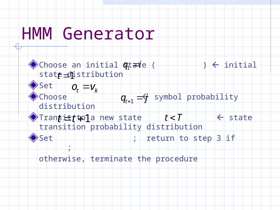
HMM Generator
Choose an initial state ( ) initial state distributionSet Choose symbol probability distributionTransit to a new state state transition probability distributionSet ; return to step 3 if ;otherwise, terminate the procedure
1q i1t t ko v
1tq j
1t t t T

HMM Properties
Often simplified , and
Obviously for all i
Discrete HMMs :
Continuous HMMs :
1( ) 1s 1( ) 0is
1ijja
1 2{ , ,... }MV v v v
dVR

HMM Properties (2)
The term “hidden” - we can only access to visible symbols (observations)- drawing conclusions without knowing the hidden sequence of states
Causal: Probabilities depend on previous states
Ergodic if every state is visited in transition sequence for any given initial state
Final or absorbing state: the state which, if entered, is never left

3 Basic Problems
The Evaluation Problem- given an HMM - given an observation- compute the probability of the observation
1 2{ , ,... | }Tp o o o
1 2, ,... To o o

3 Basic Problems (2)
The Decoding Problem- given an HMM- given an observation - compute the most likely state sequence
i.e.
1 2, ,... To o o
1 2, ,...,q q qTs s s
1,... 1 2 1argmax ( , ,..., | ,... , )q qT T Tp o o o q q

3 Basic Problems (3)
The learning / optimization problem - given an HMM - given an observation - find an HMM such that
1 2, ,... To o o
1 2 1 1 2{ , ,... | } { , ,... | }T Tp o o o p o o o

The Evaluation Problem
We know :
=
- From this :
=
1 2 1 2( , ,... | , , ,..., )T q q qTp o o o s s s
1 1 1 11 11,... 1( ) ( ) ( )
k k kq q q q q kk Ts b o a b o
1 2( , ,... | )Tp o o o
1 1 1 112
3
1 11,... 1,... 11,...1,...
1,...
( ) ( ) ( )k k k
T
q q q q q kq N k Tq Nq N
q N
s b o a b o

The Evaluation Problem(2)
Obvious:for sufficiently large values of T, it is infeasible to compute the above term for all possible state sequences need other solution

The Forward Algorithm
At time t and state i, probability of partial observation sequence
: array
1 2, ,... to o o ( )t i
1 1( ) ( )i ii b o 1 i N
[ ][ ]time state
1 11
( ) [ ( ) ] ( )N
t t ij j ti
j i a b o

The Forward Algorithm (2)
As a result at the last time T
[ ][ ] ( )timetime state state
[ ][ ]state
T state1 2( , ,... | )Tp o o o

Figure

The Backward Algorithm
1 2
1 11
1 2 11
, ,... ( )
( ) 1
( ) ( ) ( )
1, 2,...1
( , ,... | ) ( )
t t T t
T
N
t ij j t tj
N
Tj
o o o i
i
i a b o j
t T T
p o o o j

Figure

The Decoding Problem
Finding the “optimal” state sequence associated with the given observation sequence

Forward-Backward
Optimality criterion : to choose the states that are individually most likely at each time t
The probability of being in state i at time t
: accounts for partial observation sequence : account for remainder
tq
1
( ) ( | , )
( ) ( )
( ) ( )
i t
t tN
t ti
t p q i O
i i
i i
( )t i( )t i 1 2, ,...t t To o o
1 2, ,... to o o

The Viterbi Algorithm
The best score along a single path, at time t, which accounts for the first t observations and ends in state i
Keep track of the argument that maximize above equation
Viterbi Algorithm is similar in implementation to the forward calculation, but the major difference is the maximization over previous states
1 1( ) [max ( ) ] ( )t t ij j ti
j i a b o
( )t j

The Complete Procedure (for finding the best state sequence)
Initialization
Recursion
1 1
1
( ) ( )
( ) 0i ii b o
i
1 i N
11
11
( ) max[ ( ) ] ( )
( ) argmax[ ( ) ]
t t ij j ti N
t t iji N
j i a b o
j i a
2
1
t T
j N

The Complete Procedure (2)(for finding the best state sequence)
Termination
Path(state sequence) backtracking
*
1
*
1
max[ ( )]
argmax[ ( )]
Ti N
T Ti N
P i
q i
* *1 1( )
1, 2,...,1t t tq q
t T T

The Learning / Optimization problem
How do we adjust the model parameters to maximize ??
- Parameter Estimation- Baum-Welch Algorithm ( EM : Expectation
Maximization )- Iterative Procedure
( | )P O

Parameter Estimation
Probability of being in state i at time t, and state j at time t+1
1
1 1
1 11 1
( , ) ( , | , )
( ) ( ) ( )
( ) ( ) ( )
t t t
t ij j t t
N N
t ij j t ti j
i j P q i q j O
i a b o j
i a b o j

Figure

Parameter Estimation (2)
Probability of being in state i at time t, given the entire observation sequence and the model
We can relate these by summing over j
1
( ) ( , )N
t tj
i i j

Parameter Estimation (3)
By summing over time index t …- expected number of times that state i visited- expected number of transitions made from state i
• That is …
= expected number of times that state i in O
= expected number of transitions made from state i to j in O
1
1
( )T
tt
i
1
1
( , )T
tt
i j

Parameter Estimation (4)
Update using &
: expected frequency (number of times) in state i at time (t=1)
( , , )A B ( , )t i j ( )i t
_
1( )i i

Parameter Estimation (5)
New Transition Probability …
expected number of transitions from state i to j
expected number of transitions from state I
=
1
_11
1
( , )
( )
T
tt
ij T
tt
i ja
i

Parameter Estimation (6)
New Observation Probability…
expected number of times in state j and observing symbol
expected number of times in j
=
kv
1_. .
1
( )
( )( )
t k
T
tts t o v
j T
tt
j
b kj

Parameter Estimation (7)
From , if we define new
- New model is more likely than old model in the sense that
- The observation sequence is more likely to be produced by new model- has been proved by Baum & his colleagues- iteratively use new model in place of old model, and repeat the reestimation calculation “ML estimation”
( , , )A B _ _ _ _
( , , )A B
_
( | ) ( | )P O P O
Questions??