Functions and Models 1

11

Functions and Models

The fundamental objects that we deal with in calculus are functions. This chapterprepares the way for calculus by discussing the basic ideas concerning functions,their graphs, and ways of transforming and combining them. We stress that afunction can be represented in different ways: by an equation, in a table, by agraph, or in words. We look at the main types of functions that occur in calculusand describe the process of using these functions as mathematical models ofreal-world phenomena. We also discuss the use of graphing calculators andgraphing software for computers and see that parametric equations provide thebest method for graphing certain types of curves.

1thomasmayerarchive.com

57425_01_ch01_p010-021.qk 11/21/08 9:44 AM Page 11

12 CHAPTER 1 FUNCTIONS AND MODELS

Functions arise whenever one quantity depends on another. Consider the following foursituations.

A. The area of a circle depends on the radius of the circle. The rule that connects and is given by the equation . With each positive number there is associ-ated one value of , and we say that is a function of .

B. The human population of the world depends on the time . The table gives estimatesof the world population at time for certain years. For instance,

But for each value of the time there is a corresponding value of and we say that is a function of .

C. The cost of mailing a large envelope depends on the weight of the envelope.Although there is no simple formula that connects and , the post office has a rulefor determining when is known.

D. The vertical acceleration of the ground as measured by a seismograph during anearthquake is a function of the elapsed time Figure 1 shows a graph generated byseismic activity during the Northridge earthquake that shook Los Angeles in 1994.For a given value of the graph provides a corresponding value of .

Each of these examples describes a rule whereby, given a number ( , , , or ), anothernumber ( , , , or ) is assigned. In each case we say that the second number is a func-tion of the first number.

A function is a rule that assigns to each element in a set exactly one ele-ment, called , in a set .

We usually consider functions for which the sets and are sets of real numbers. Theset is called the domain of the function. The number is the value of at and isread “ of .” The range of is the set of all possible values of as varies through-out the domain. A symbol that represents an arbitrary number in the domain of a function

is called an independent variable. A symbol that represents a number in the range of is called a dependent variable. In Example A, for instance, r is the independent variableand A is the dependent variable.

ff

xf �x�fxfxff �x�D

ED

Ef �x�Dxf

aCPAtwtr

FIGURE 1Vertical ground acceleration during

the Northridge earthquake

{cm/s@}

(seconds)

Calif. Dept. of Mines and Geology

5

50

10 15 20 25

a

t

100

30

_50

at,

t.a

wCCw

wC

tPP,t

P�1950� � 2,560,000,000

t,P�t�tP

rAArA � �r 2A

rrA

1.1 Four Ways to Represent a Function

PopulationYear (millions)

1900 16501910 17501920 18601930 20701940 23001950 25601960 30401970 37101980 44501990 52802000 6080

57425_01_ch01_p010-021.qk 11/21/08 9:44 AM Page 12

SECTION 1.1 FOUR WAYS TO REPRESENT A FUNCTION 13

It’s helpful to think of a function as a machine (see Figure 2). If is in the domain ofthe function then when enters the machine, it’s accepted as an input and the machineproduces an output according to the rule of the function. Thus we can think of thedomain as the set of all possible inputs and the range as the set of all possible outputs.

The preprogrammed functions in a calculator are good examples of a function as amachine. For example, the square root key on your calculator computes such a function.You press the key labeled (or ) and enter the input . If , then is not in thedomain of this function; that is, is not an acceptable input, and the calculator will indi-cate an error. If , then an approximation to will appear in the display. Thus the

key on your calculator is not quite the same as the exact mathematical function defined by .

Another way to picture a function is by an arrow diagram as in Figure 3. Each arrowconnects an element of to an element of . The arrow indicates that is associatedwith is associated with , and so on.

The most common method for visualizing a function is its graph. If is a function withdomain , then its graph is the set of ordered pairs

(Notice that these are input-output pairs.) In other words, the graph of consists of allpoints in the coordinate plane such that and is in the domain of .

The graph of a function gives us a useful picture of the behavior or “life history” ofa function. Since the -coordinate of any point on the graph is , we can readthe value of from the graph as being the height of the graph above the point (seeFigure 4). The graph of also allows us to picture the domain of on the -axis and itsrange on the -axis as in Figure 5.

Reading information from a graph The graph of a function is shown in Figure 6.(a) Find the values of and .(b) What are the domain and range of ?

SOLUTION(a) We see from Figure 6 that the point lies on the graph of , so the value ofat 1 is . (In other words, the point on the graph that lies above is 3 unitsabove the -axis.)

When , the graph lies about 0.7 unit below the x-axis, so we estimate that.

(b) We see that is defined when , so the domain of is the closed inter-val . Notice that takes on all values from to 4, so the range of is

�y � �2 � y � 4� � ��2, 4

f�2f�0, 7f0 � x � 7f �x�

f �5� � �0.7x � 5x

x � 1f �1� � 3ff�1, 3�

ff �5�f �1�

fEXAMPLE 1

0

y � ƒ(x)

domain

range

FIGURE 4

{x, ƒ}

ƒ

f(1)f(2)

0 1 2 x

FIGURE 5

xx

y y

yxff

xf �x�y � f �x��x, y�y

ffxy � f �x��x, y�

f

��x, f �x�� x � D�

Df

af �a�x,f �x�ED

f �x� � sx fsx

sx x � 0x

xx � 0xsx s

f �x�xf,

x

FIGURE 2Machine diagram for a function ƒ

x(input)

ƒ(output)

f

fD E

ƒ

f(a)a

x

FIGURE 3 Arrow diagram for ƒ

FIGURE 6

x

y

0

1

1

The notation for intervals is given in Appendix A.

57425_01_ch01_p010-021.qk 11/21/08 9:44 AM Page 13


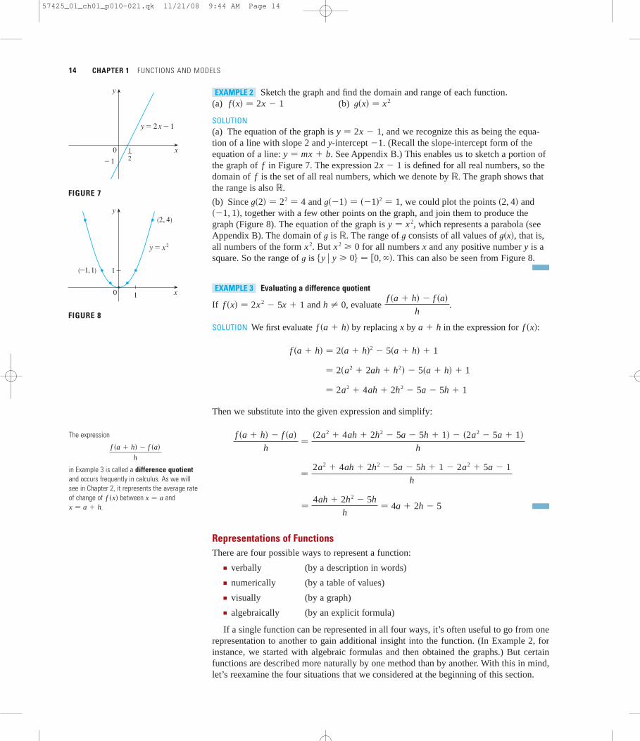
Sketch the graph and find the domain and range of each function.(a) (b)

SOLUTION(a) The equation of the graph is , and we recognize this as being the equa-tion of a line with slope 2 and -intercept . (Recall the slope-intercept form of theequation of a line: . See Appendix B.) This enables us to sketch a portion ofthe graph of in Figure 7. The expression is defined for all real numbers, so thedomain of is the set of all real numbers, which we denote by . The graph shows thatthe range is also .

(b) Since and , we could plot the points and, together with a few other points on the graph, and join them to produce the

graph (Figure 8). The equation of the graph is , which represents a parabola (seeAppendix B). The domain of is . The range of consists of all values of , that is,all numbers of the form . But for all numbers and any positive number is asquare. So the range of is . This can also be seen from Figure 8.

Evaluating a difference quotient

If and , evaluate .

SOLUTION We first evaluate by replacing by in the expression for :

Then we substitute into the given expression and simplify:

Representations of FunctionsThere are four possible ways to represent a function:

■ verbally (by a description in words)

■ numerically (by a table of values)

■ visually (by a graph)

■ algebraically (by an explicit formula)

If a single function can be represented in all four ways, it’s often useful to go from onerepresentation to another to gain additional insight into the function. (In Example 2, forinstance, we started with algebraic formulas and then obtained the graphs.) But certainfunctions are described more naturally by one method than by another. With this in mind,let’s reexamine the four situations that we considered at the beginning of this section.

�4ah � 2h2 � 5h

h� 4a � 2h � 5

�2a2 � 4ah � 2h2 � 5a � 5h � 1 � 2a2 � 5a � 1

h

f �a � h� � f �a�h

��2a2 � 4ah � 2h2 � 5a � 5h � 1� � �2a2 � 5a � 1�

h

� 2a2 � 4ah � 2h2 � 5a � 5h � 1

� 2�a2 � 2ah � h2� � 5�a � h� � 1

f �a � h� � 2�a � h�2 � 5�a � h� � 1

f �x�a � hxf �a � h�

f �a � h� � f �a�h

h � 0f �x� � 2x 2 � 5x � 1

EXAMPLE 3

�y � y � 0� � �0, ��t

yxx 2 � 0x 2t�x�t�t

y � x 2��1, 1�

�2, 4�t��1� � ��1�2 � 1t�2� � 22 � 4

�

�f2x � 1f

y � mx � b�1y

y � 2x � 1

t�x� � x 2f �x� � 2x � 1EXAMPLE 2

The expression

in Example 3 is called a difference quotientand occurs frequently in calculus. As we will see in Chapter 2, it represents the average rate of change of between and

.x � a � hx � af �x�

f �a � h� � f �a�h

FIGURE 7

x

y=2x-1

0-1

y

12

(_1, 1)

(2, 4)

0

y

1

x1

y=≈

FIGURE 8

57425_01_ch01_p010-021.qk 11/21/08 9:44 AM Page 14


A. The most useful representation of the area of a circle as a function of its radius isprobably the algebraic formula , though it is possible to compile a table ofvalues or to sketch a graph (half a parabola). Because a circle has to have a positiveradius, the domain is , and the range is also .

B. We are given a description of the function in words: is the human population ofthe world at time t. The table of values of world population provides a convenientrepresentation of this function. If we plot these values, we get the graph (called ascatter plot) in Figure 9. It too is a useful representation; the graph allows us toabsorb all the data at once. What about a formula? Of course, it’s impossible to devisean explicit formula that gives the exact human population at any time t. But it ispossible to find an expression for a function that approximates . In fact, usingmethods explained in Section 1.5, we obtain the approximation

and Figure 10 shows that it is a reasonably good “fit.” The function is called amathematical model for population growth. In other words, it is a function with anexplicit formula that approximates the behavior of our given function. We will see,however, that the ideas of calculus can be applied to a table of values; an explicitformula is not necessary.

The function is typical of the functions that arise whenever we attempt to applycalculus to the real world. We start with a verbal description of a function. Then wemay be able to construct a table of values of the function, perhaps from instrumentreadings in a scientific experiment. Even though we don’t have complete knowledgeof the values of the function, we will see throughout the book that it is still possible toperform the operations of calculus on such a function.

C. Again the function is described in words: is the cost of mailing a large envelopewith weight . The rule that the US Postal Service used as of 2008 is as follows: Thecost is 83 cents for up to 1 oz, plus 17 cents for each additional ounce (or less) up to13 oz. The table of values shown in the margin is the most convenient representationfor this function, though it is possible to sketch a graph (see Example 10).

D. The graph shown in Figure 1 is the most natural representation of the vertical acceler-ation function . It’s true that a table of values could be compiled, and it is even possible to devise an approximate formula. But everything a geologist needs toknow—amplitudes and patterns—can be seen easily from the graph. (The same is true for the patterns seen in electrocardiograms of heart patients and polygraphs forlie-detection.)

a�t�

wC�w�

P

FIGURE 10FIGURE 9

1900

6x10'

P

t1920 1940 1960 1980 2000 1900

6x10'

P

t1920 1940 1960 1980 2000

f

P�t� � f �t� � �0.008079266� �1.013731�t

P�t�P�t�

P�t�

�0, ��r � r 0� � �0, ��

A�r� � �r 2


1900 16501910 17501920 18601930 20701940 23001950 25601960 30401970 37101980 44501990 52802000 6080

(ounces) (dollars)

0.831.001.171.341.51

2.8712 � w � 13

4 � w � 53 � w � 42 � w � 31 � w � 20 � w � 1

C�w�w

A function defined by a table of values is called atabular function.

57425_01_ch01_p010-021.qk 11/21/08 9:44 AM Page 15


Drawing a graph from a verbal description When you turn on a hot-waterfaucet, the temperature of the water depends on how long the water has been running.Draw a rough graph of as a function of the time that has elapsed since the faucet wasturned on.

SOLUTION The initial temperature of the running water is close to room temperaturebecause the water has been sitting in the pipes. When the water from the hot-water tankstarts flowing from the faucet, increases quickly. In the next phase, is constant atthe temperature of the heated water in the tank. When the tank is drained, decreases to the temperature of the water supply. This enables us to make the rough sketch of asa function of in Figure 11.

In the following example we start with a verbal description of a function in a physicalsituation and obtain an explicit algebraic formula. The ability to do this is a useful skill insolving calculus problems that ask for the maximum or minimum values of quantities.

Expressing a cost as a function A rectangular storage container with anopen top has a volume of 10 m . The length of its base is twice its width. Material forthe base costs $10 per square meter; material for the sides costs $6 per square meter.Express the cost of materials as a function of the width of the base.

SOLUTION We draw a diagram as in Figure 12 and introduce notation by letting andbe the width and length of the base, respectively, and be the height.

The area of the base is , so the cost, in dollars, of the material for thebase is . Two of the sides have area and the other two have area , so thecost of the material for the sides is . The total cost is therefore

To express as a function of alone, we need to eliminate and we do so by using thefact that the volume is 10 m . Thus

which gives

Substituting this into the expression for , we have

Therefore the equation

expresses as a function of .

Find the domain of each function.

(a) (b)

SOLUTION(a) Because the square root of a negative number is not defined (as a real number), the domain of consists of all values of such that . This is equivalent to

, so the domain is the interval .��2, ��x � �2x � 2 � 0xf

t�x� �1

x 2 � xf �x� � sx � 2

EXAMPLE 6

wC

w 0C�w� � 20w2 �180

w

C � 20w2 � 36w 5

w2� � 20w2 �180

w

C

h �10

2w2 �5

w2

w�2w�h � 10

3hwC

C � 10�2w2 � � 6�2�wh� � 2�2wh� � 20w2 � 36wh

6�2�wh� � 2�2wh�2whwh10�2w2 �

�2w�w � 2w2h

2ww

3EXAMPLE 5v

tT

TTT

tTT

EXAMPLE 4

t

T

0

FIGURE 11

w

2w

h

FIGURE 12

In setting up applied functions as in Example 5, it may be useful to review the principles of problem solving as discussed onpage 83, particularly Step 1: Understand theProblem.

PS

Domain ConventionIf a function is given by a formula and thedomain is not stated explicitly, the convention isthat the domain is the set of all numbers forwhich the formula makes sense and defines areal number.

57425_01_ch01_p010-021.qk 11/21/08 9:44 AM Page 16


(b) Since

and division by is not allowed, we see that is not defined when or .Thus the domain of is

which could also be written in interval notation as

The graph of a function is a curve in the -plane. But the question arises: Which curvesin the -plane are graphs of functions? This is answered by the following test.

The Vertical Line Test A curve in the -plane is the graph of a function of if andonly if no vertical line intersects the curve more than once.

The reason for the truth of the Vertical Line Test can be seen in Figure 13. If each ver-tical line intersects a curve only once, at , then exactly one functional value is defined by . But if a line intersects the curve twice, at and ,then the curve can’t represent a function because a function can’t assign two different val-ues to .

For example, the parabola shown in Figure 14(a) is not the graph of a func-tion of because, as you can see, there are vertical lines that intersect the parabola twice.The parabola, however, does contain the graphs of two functions of . Notice that the equa-tion implies , so Thus the upper and lower halvesof the parabola are the graphs of the functions [from Example 6(a)] and

. [See Figures 14(b) and (c).] We observe that if we reverse the roles ofand , then the equation does define as a function of (with as

the independent variable and as the dependent variable) and the parabola now appears asthe graph of the function .

FIGURE 14 (b) y=œ„„„„x+2

_2 0 x

y

(_2, 0)

(a) x=¥-2

0 x

y

(c) y=_œ„„„„x+2

_20

y

x

hx

yy xx � h�y� � y 2 � 2yxt�x� � �sx � 2

f �x� � sx � 2

y � �sx � 2 .y 2 � x � 2x � y 2 � 2x

xx � y 2 � 2

a

x=a

(a, b)

0 a

(a, c)

(a, b)

x=a

0 x

y

x

y

FIGURE 13

a

�a, c��a, b�x � af �a� � b�a, b�x � a

xxy

xyxy

��, 0� � �0, 1� � �1, ��

�x � x � 0, x � 1�

t

x � 1x � 0t�x�0

t�x� �1

x 2 � x�

1

x�x � 1�

57425_01_ch01_p010-021.qk 11/21/08 9:44 AM Page 17


Piecewise Defined FunctionsThe functions in the following four examples are defined by different formulas in differ-ent parts of their domains.

Graphing a piecewise defined function A function is defined by

Evaluate , , and and sketch the graph.

SOLUTION Remember that a function is a rule. For this particular function the rule is thefollowing: First look at the value of the input . If it happens that , then the valueof is . On the other hand, if , then the value of is .

How do we draw the graph of ? We observe that if , then , so the part of the graph of that lies to the left of the vertical line must coincidewith the line , which has slope and -intercept 1. If , then ,so the part of the graph of that lies to the right of the line must coincide with thegraph of , which is a parabola. This enables us to sketch the graph in Figure 15.The solid dot indicates that the point is included on the graph; the open dot indi-cates that the point is excluded from the graph.

The next example of a piecewise defined function is the absolute value function. Recallthat the absolute value of a number , denoted by , is the distance from to on thereal number line. Distances are always positive or , so we have

for every number

For example,

In general, we have

(Remember that if is negative, then is positive.)

Sketch the graph of the absolute value function .

SOLUTION From the preceding discussion we know that

Using the same method as in Example 7, we see that the graph of coincides with theline to the right of the -axis and coincides with the line to the left of the-axis (see Figure 16).y

y � �xyy � xf

� x � � �x

�x

if x � 0

if x � 0

f �x� � � x �EXAMPLE 8

�aa

if a � 0� a � � �a

if a � 0� a � � a

� 3 � � � � � � 3� s2 � 1 � � s2 � 1� 0 � � 0� �3 � � 3� 3 � � 3

a� a � � 0

00a� a �a

�1, 1��1, 0�

y � x 2x � 1f

f �x� � x 2x 1y�1y � 1 � xx � 1f

f �x� � 1 � xx � 1f

Since 2 1, we have f �2� � 22 � 4.

Since 1 � 1, we have f �1� � 1 � 1 � 0.

Since 0 � 1, we have f �0� � 1 � 0 � 1.

x 2f �x�x 11 � xf �x�� 1xx

f �2�f �1�f �0�

f �x� � �1 � x

x 2

if x � 1

if x 1

fEXAMPLE 7v

1

x

y

1

FIGURE 15

x

y=| x |

0

y

FIGURE 16

For a more extensive review of absolute values,see Appendix A.

57425_01_ch01_p010-021.qk 11/21/08 9:44 AM Page 18


Find a formula for the function graphed in Figure 17.

SOLUTION The line through and has slope and -intercept , soits equation is . Thus, for the part of the graph of that joins to , wehave

The line through and has slope , so its point-slope form is

So we have

We also see that the graph of coincides with the -axis for . Putting this informa-tion together, we have the following three-piece formula for :

Graph of a postage function In Example C at the beginning of this sectionwe considered the cost of mailing a large envelope with weight . In effect, this isa piecewise defined function because, from the table of values on page 15, we have

The graph is shown in Figure 18. You can see why functions similar to this one arecalled step functions—they jump from one value to the next. Such functions will bestudied in Chapter 2.

SymmetryIf a function satisfies for every number in its domain, then is called aneven function. For instance, the function is even because

The geometric significance of an even function is that its graph is symmetric with respect

f ��x� � ��x�2 � x 2 � f �x�

f �x� � x 2fxf ��x� � f �x�f

��

0.83

1.00

1.17

1.34

if 0 � w � 1

if 1 � w � 2

if 2 � w � 3

if 3 � w � 4C�w� �

wC�w�EXAMPLE 10

f �x� � �x

2 � x

0

if 0 � x � 1

if 1 � x � 2

if x � 2

fx � 2xf

if 1 � x � 2f �x� � 2 � x

y � 2 � xory � 0 � ��1��x � 2�

m � �1�2, 0��1, 1�

if 0 � x � 1f �x� � x

�1, 1��0, 0�fy � xb � 0ym � 1�1, 1��0, 0�

FIGURE 17x

y

0 1

1

fEXAMPLE 9

Point-slope form of the equation of a line:

See Appendix B.

y � y1 � m�x � x1 �

FIGURE 18

C

0.50

1.00

1.50

0 1 2 3 54 w

57425_01_ch01_p011-021.qk 4/2/09 11:32 AM Page 19


to the -axis (see Figure 19). This means that if we have plotted the graph of for ,we obtain the entire graph simply by reflecting this portion about the -axis.

If satisfies for every number in its domain, then is called an oddfunction. For example, the function is odd because

The graph of an odd function is symmetric about the origin (see Figure 20). If we alreadyhave the graph of for , we can obtain the entire graph by rotating this portionthrough about the origin.

Determine whether each of the following functions is even, odd, or neither even nor odd.(a) (b) (c)

SOLUTION

(a)

Therefore is an odd function.

(b)

So is even.

(c)

Since and , we conclude that is neither even nor odd.

The graphs of the functions in Example 11 are shown in Figure 21. Notice that thegraph of h is symmetric neither about the y-axis nor about the origin.

FIGURE 21

1

1 x

y

h1

1

y

x

g1

_1

1

y

x

f

_1

(a) (b) (c)

hh��x� � �h�x�h��x� � h�x�

h��x� � 2��x� � ��x�2 � �2x � x 2

t

t��x� � 1 � ��x�4 � 1 � x 4 � t�x�

f

� �f �x�

� �x 5 � x � ��x 5 � x�

f ��x� � ��x�5 � ��x� � ��1�5x 5 � ��x�

h�x� � 2x � x 2t�x� � 1 � x 4f �x� � x 5 � x

EXAMPLE 11v

180�x � 0f

f ��x� � ��x�3 � �x 3 � �f �x�

f �x� � x 3fxf ��x� � �f �x�f

0x

_x ƒ

FIGURE 20 An odd function

x

y

0 x_x

f(_x) ƒ

An even function

x

FIGURE 19

y

yx � 0fy

57425_01_ch01_p010-021.qk 11/21/08 9:44 AM Page 20


Increasing and Decreasing FunctionsThe graph shown in Figure 22 rises from to , falls from to , and rises again from to . The function is said to be increasing on the interval , decreasing on , andincreasing again on . Notice that if and are any two numbers between and with , then . We use this as the defining property of an increasingfunction.

A function is called increasing on an interval if

It is called decreasing on if

In the definition of an increasing function it is important to realize that the inequalitymust be satisfied for every pair of numbers and in with .

You can see from Figure 23 that the function is decreasing on the intervaland increasing on the interval .�0, ��, 0

f �x� � x 2x1 � x2Ix2x1f �x1 � � f �x2 �

whenever x1 � x2 in If �x1 � f �x2 �

I

whenever x1 � x2 in If �x1 � � f �x2 �

If

f �x1 � � f �x2 �x1 � x2

bax2x1�c, d �b, c�a, bfD

CCBBA

A

B

C

D

y=ƒ

f(x¡)

a

y

0 xx¡ x™ b c d

FIGURE 22

f(x™)

FIGURE 23

0

y

x

y=≈

1.1 Exercises

1. The graph of a function is given.

(a) State the value of .

(b) Estimate the value of .

(c) For what values of is ?

(d) Estimate the value of such that .

(e) State the domain and range of .

(f) On what interval is increasing?

2. The graphs of and t are given.

(a) State the values of and .

(b) For what values of is ?

(c) Estimate the solution of the equation .

(d) On what interval is decreasing?f

f �x� � �1

f �x� � t�x�x

t�3�f ��4�f

y

0 x1

1

f

f

f �x� � 0x

f �x� � 1x

f ��1�f �1�

f (e) State the domain and range of

(f) State the domain and range of .

3. Figure 1 was recorded by an instrument operated by the Cali-fornia Department of Mines and Geology at the UniversityHospital of the University of Southern California in Los Ange-les. Use it to estimate the range of the vertical ground accelera-tion function at USC during the Northridge earthquake.

4. In this section we discussed examples of ordinary, everydayfunctions: Population is a function of time, postage cost is afunction of weight, water temperature is a function of time.Give three other examples of functions from everyday life thatare described verbally. What can you say about the domain andrange of each of your functions? If possible, sketch a roughgraph of each function.

g

x

y

0

f2

2

t

f.

1. Homework Hints available in TEC

57425_01_ch01_p010-021.qk 11/21/08 9:44 AM Page 21


5–8 Determine whether the curve is the graph of a function of . If it is, state the domain and range of the function.

5. 6.

7. 8.

9. The graph shown gives the weight of a certain person as afunction of age. Describe in words how this person’s weightvaries over time. What do you think happened when this personwas 30 years old?

10. The graph shows the height of the water in a bathtub as a function of time. Give a verbal description of what you thinkhappened.

11. You put some ice cubes in a glass, fill the glass with coldwater, and then let the glass sit on a table. Describe how thetemperature of the water changes as time passes. Then sketch arough graph of the temperature of the water as a function of theelapsed time.

12. Three runners compete in a 100-meter race. The graph depictsthe distance run as a function of time for each runner. Describe

0

height(inches)

15

10

5

time(min)

5 10 15

age(years)

weight(pounds)

0

150

100

50

10

200

20 30 40 50 60 70

y

x0 1

1

y

x0

1

1

y

x0 1

1

y

x0 1

1

x in words what the graph tells you about this race. Who won therace? Did each runner finish the race?

13. The graph shows the power consumption for a day in Septem-ber in San Francisco. ( is measured in megawatts; is mea-sured in hours starting at midnight.)(a) What was the power consumption at 6 AM? At 6 PM?(b) When was the power consumption the lowest? When was it

the highest? Do these times seem reasonable?

14. Sketch a rough graph of the number of hours of daylight as afunction of the time of year.

15. Sketch a rough graph of the outdoor temperature as a functionof time during a typical spring day.

16. Sketch a rough graph of the market value of a new car as afunction of time for a period of 20 years. Assume the car iswell maintained.

17. Sketch the graph of the amount of a particular brand of coffeesold by a store as a function of the price of the coffee.

18. You place a frozen pie in an oven and bake it for an hour. Thenyou take it out and let it cool before eating it. Describe how thetemperature of the pie changes as time passes. Then sketch arough graph of the temperature of the pie as a function of time.

19. A homeowner mows the lawn every Wednesday afternoon.Sketch a rough graph of the height of the grass as a function oftime over the course of a four-week period.

20. An airplane takes off from an airport and lands an hour later atanother airport, 400 miles away. If t represents the time in min-utes since the plane has left the terminal building, let be x�t�

P

0 181512963 t21

400

600

800

200

Pacific Gas & Electric

tP

0

y (m)

100

t (s)20

A B C

57425_01_ch01_p022-031.qk 11/21/08 9:47 AM Page 22


the horizontal distance traveled and be the altitude of theplane.(a) Sketch a possible graph of .(b) Sketch a possible graph of .(c) Sketch a possible graph of the ground speed.(d) Sketch a possible graph of the vertical velocity.

21. The number N (in millions) of US cellular phone subscribers isshown in the table. (Midyear estimates are given.)

(a) Use the data to sketch a rough graph of N as a function of (b) Use your graph to estimate the number of cell-phone sub-

scribers at midyear in 2001 and 2005.

22. Temperature readings (in °F) were recorded every two hoursfrom midnight to 2:00 PM in Baltimore on September 26, 2007.The time was measured in hours from midnight.

(a) Use the readings to sketch a rough graph of as a functionof

(b) Use your graph to estimate the temperature at 11:00 AM.

23. If , find , , , ,, , , , and .

24. A spherical balloon with radius r inches has volume. Find a function that represents the amount of air

required to inflate the balloon from a radius of r inches to aradius of r � 1 inches.

25–28 Evaluate the difference quotient for the given function. Simplify your answer.

25. ,

26. ,

27. ,

28. ,

29–33 Find the domain of the function.

29. 30.

31. 32. t�t� � s3 � t � s2 � t f �t� � s3 2t � 1

f �x� �2x 3 � 5

x 2 � x � 6f �x� �

x � 4

x 2 � 9

f �x� � f �1�x � 1

f �x� �x � 3

x � 1

f �x� � f �a�x � a

f �x� �1

x

f �a � h� � f �a�h

f �x� � x 3

f �3 � h� � f �3�h

f �x� � 4 � 3x � x 2

V�r� � 43 �r 3

f �a � h�[ f �a�]2, f �a2� f �2a�2 f �a�f �a � 1� f ��a� f �a� f ��2�f �2�f �x� � 3x 2 � x � 2

t.T

t

T

t.

y�t�x�t�

y�t�33.

34. Find the domain and range and sketch the graph of the function .

35–46 Find the domain and sketch the graph of the function.

35. 36.

37. 38.

39. 40.

41. 42.

43.

44.

45.

46.

47–52 Find an expression for the function whose graph is the given curve.

47. The line segment joining the points and

48. The line segment joining the points and

49. The bottom half of the parabola

50. The top half of the circle

51. 52.

53–57 Find a formula for the described function and state itsdomain.

53. A rectangle has perimeter 20 m. Express the area of the rect-angle as a function of the length of one of its sides.

54. A rectangle has area 16 m . Express the perimeter of the rect-angle as a function of the length of one of its sides.

2

y

0 x

1

1

y

0 x

1

1

x 2 � �y � 2�2 � 4

x � �y � 1�2 � 0

�7, �10��5, 10�

�5, 7��1, �3�

f �x� � �x � 9

�2x

�6

if x � �3

if � x � � 3

if x � 3

f �x� � �x � 2

x 2

if x � �1

if x � �1

f �x� � �3 �12 x

2x � 5

if x � 2

if x � 2

f �x� � �x � 2

1 � x

if x � 0

if x � 0

t�x� � � x � � xG�x� �3x � � x �

x

F�x� � � 2x � 1 �t�x� � sx � 5

H�t� �4 � t 2

2 � tf �t� � 2t � t 2

F �x� � x 2 � 2x � 1f �x� � 2 � 0.4x

h�x� � s4 � x 2

h�x� �1

s4 x 2 � 5x

t 1996 1998 2000 2002 2004 2006

N 44 69 109 141 182 233

t 0 2 4 6 8 10 12 14

T 68 65 63 63 65 76 85 91

57425_01_ch01_p022-031.qk 11/21/08 9:47 AM Page 23


55. Express the area of an equilateral triangle as a function of thelength of a side.

56. Express the surface area of a cube as a function of its volume.

57. An open rectangular box with volume 2 m has a square base.Express the surface area of the box as a function of the lengthof a side of the base.

58. A Norman window has the shape of a rectangle surmounted bya semicircle. If the perimeter of the window is 30 ft, expressthe area of the window as a function of the width of thewindow.

59. A box with an open top is to be constructed from a rectangularpiece of cardboard with dimensions 12 in. by 20 in. by cuttingout equal squares of side at each corner and then folding upthe sides as in the figure. Express the volume of the box as afunction of .

60. An electricity company charges its customers a base rate of $10a month, plus 6 cents per kilowatt-hour (kWh) for the first1200 kWh and 7 cents per kWh for all usage over 1200 kWh.Express the monthly cost as a function of the amount ofelectricity used. Then graph the function for .

61. In a certain country, income tax is assessed as follows. There isno tax on income up to $10,000. Any income over $10,000 istaxed at a rate of 10%, up to an income of $20,000. Any incomeover $20,000 is taxed at 15%.(a) Sketch the graph of the tax rate R as a function of the

income I.(b) How much tax is assessed on an income of $14,000?

On $26,000?(c) Sketch the graph of the total assessed tax T as a function of

the income I.

0 � x � 2000ExE

20

12x

x

x

x

x x

x x

xV

x

x

xA

3

62. The functions in Example 10 and Exercise 61(a) are called step functions because their graphs look like stairs. Give twoother examples of step functions that arise in everyday life.

63–64 Graphs of and are shown. Decide whether each functionis even, odd, or neither. Explain your reasoning.

63. 64.

65. (a) If the point is on the graph of an even function, whatother point must also be on the graph?

(b) If the point is on the graph of an odd function, whatother point must also be on the graph?

66. A function has domain and a portion of its graph isshown.(a) Complete the graph of if it is known that is even.(b) Complete the graph of if it is known that is odd.

67–72 Determine whether is even, odd, or neither. If you have agraphing calculator, use it to check your answer visually.

67. 68.

69. 70.

71. 72.

73. If and are both even functions, is even? If and areboth odd functions, is odd? What if is even and isodd? Justify your answers.

74. If and are both even functions, is the product even? If and are both odd functions, is odd? What if is even and is odd? Justify your answers.

tfftt

ffttf

tff � t

tff � ttf

f �x� � 1 � 3x 3 � x 5f �x� � 1 � 3x 2 � x 4

f �x� � x � x �f �x� �x

x � 1

f �x� �x 2

x 4 � 1f �x� �

x

x 2 � 1

f

x0

y

5_5

ffff

��5, 5�f

�5, 3�

�5, 3�

y

x

f

g

y

x

f

g

tf

57425_01_ch01_p022-031.qk 11/21/08 9:47 AM Page 24

SECTION 1.2 MATHEMATICAL MODELS: A CATALOG OF ESSENTIAL FUNCTIONS 25

A mathematical model is a mathematical description (often by means of a function or anequation) of a real-world phenomenon such as the size of a population, the demand for aproduct, the speed of a falling object, the concentration of a product in a chemical reac-tion, the life expectancy of a person at birth, or the cost of emission reductions. The pur-pose of the model is to understand the phenomenon and perhaps to make predictions aboutfuture behavior.

Figure 1 illustrates the process of mathematical modeling. Given a real-world problem,our first task is to formulate a mathematical model by identifying and naming the inde-pendent and dependent variables and making assumptions that simplify the phenomenonenough to make it mathematically tractable. We use our knowledge of the physical situa-tion and our mathematical skills to obtain equations that relate the variables. In situationswhere there is no physical law to guide us, we may need to collect data (either from alibrary or the Internet or by conducting our own experiments) and examine the data in theform of a table in order to discern patterns. From this numerical representation of a func-tion we may wish to obtain a graphical representation by plotting the data. The graphmight even suggest a suitable algebraic formula in some cases.

The second stage is to apply the mathematics that we know (such as the calculus thatwill be developed throughout this book) to the mathematical model that we have formu-lated in order to derive mathematical conclusions. Then, in the third stage, we take thosemathematical conclusions and interpret them as information about the original real-worldphenomenon by way of offering explanations or making predictions. The final step is totest our predictions by checking against new real data. If the predictions don’t comparewell with reality, we need to refine our model or to formulate a new model and start thecycle again.

A mathematical model is never a completely accurate representation of a physical situ-ation—it is an idealization. A good model simplifies reality enough to permit mathemati-cal calculations but is accurate enough to provide valuable conclusions. It is important torealize the limitations of the model. In the end, Mother Nature has the final say.

There are many different types of functions that can be used to model relationshipsobserved in the real world. In what follows, we discuss the behavior and graphs of these functions and give examples of situations appropriately modeled by such functions.

Linear ModelsWhen we say that y is a linear function of x, we mean that the graph of the function is aline, so we can use the slope-intercept form of the equation of a line to write a formula forthe function as

where m is the slope of the line and b is the y-intercept.

y � f �x� � mx � b

FIGURE 1 The modeling process

Real-worldproblem

Mathematicalmodel

Real-worldpredictions

Mathematicalconclusions

Test

Formulate Solve Interpret

1.2 Mathematical Models: A Catalog of Essential Functions

The coordinate geometry of lines is reviewed in Appendix B.

57425_01_ch01_p022-031.qk 11/21/08 9:47 AM Page 25


A characteristic feature of linear functions is that they grow at a constant rate. Forinstance, Figure 2 shows a graph of the linear function and a table of sam-ple values. Notice that whenever x increases by 0.1, the value of increases by 0.3. So

increases three times as fast as x. Thus the slope of the graph , namely 3, canbe interpreted as the rate of change of y with respect to x.

Interpreting the slope of a linear model(a) As dry air moves upward, it expands and cools. If the ground temperature is and the temperature at a height of 1 km is , express the temperature T (in °C) as afunction of the height h (in kilometers), assuming that a linear model is appropriate.(b) Draw the graph of the function in part (a). What does the slope represent?(c) What is the temperature at a height of 2.5 km?

SOLUTION(a) Because we are assuming that T is a linear function of h, we can write

We are given that when , so

In other words, the y-intercept is .We are also given that when , so

The slope of the line is therefore and the required linear function is

(b) The graph is sketched in Figure 3. The slope is , and this representsthe rate of change of temperature with respect to height.

(c) At a height of , the temperature is

If there is no physical law or principle to help us formulate a model, we construct anempirical model, which is based entirely on collected data. We seek a curve that “fits” thedata in the sense that it captures the basic trend of the data points.

T � �10�2.5� � 20 � �5C

h � 2.5 km

m � �10C�km

T � �10h � 20

m � 10 � 20 � �10

10 � m � 1 � 20

h � 1T � 10b � 20

20 � m � 0 � b � b

h � 0T � 20

T � mh � b

10C20C

EXAMPLE 1v

x

y

0

y=3x-2

_2

FIGURE 2

y � 3x � 2f �x�f �x�

f �x� � 3x � 2

x

1.0 1.01.1 1.31.2 1.61.3 1.91.4 2.21.5 2.5

f �x� � 3x � 2

FIGURE 3

T=_10h+20

T

h0

10

20

1 3

57425_01_ch01_p022-031.qk 11/21/08 9:47 AM Page 26


A linear regression model Table 1 lists the average carbon dioxide level inthe atmosphere, measured in parts per million at Mauna Loa Observatory from 1980 to2006. Use the data in Table 1 to find a model for the carbon dioxide level.

SOLUTION We use the data in Table 1 to make the scatter plot in Figure 4, where repre-sents time (in years) and represents the level (in parts per million, ppm).

Notice that the data points appear to lie close to a straight line, so it’s natural tochoose a linear model in this case. But there are many possible lines that approximatethese data points, so which one should we use? One possibility is the line that passesthrough the first and last data points. The slope of this line is

and its equation is

or

Equation 1 gives one possible linear model for the carbon dioxide level; it is graphedin Figure 5.

Notice that our model gives values higher than most of the actual levels. A betterlinear model is obtained by a procedure from statistics called linear regression. If we use

CO2

FIGURE 5 Linear model through

first and last data points

C

340

350

360

370

380

1980 1985 1990 t1995 2000 2005

C � 1.6615t � 2951.071

C � 338.7 � 1.6615�t � 1980�

381.9 � 338.7

2006 � 1980�

43.2

26 1.6615

C

FIGURE 4 Scatter plot for the average CO™ level

340

350

360

370

380

1980 1985 t1990 1995 2000 2005

CO2Ct

EXAMPLE 2v

TABLE 1

level levelYear (in ppm) Year (in ppm)

1980 338.7 1994 358.91982 341.1 1996 362.61984 344.4 1998 366.61986 347.2 2000 369.41988 351.5 2002 372.91990 354.2 2004 377.51992 356.4 2006 381.9

CO2CO2

57425_01_ch01_p022-031.qk 11/21/08 9:47 AM Page 27


a graphing calculator, we enter the data from Table 1 into the data editor and choose thelinear regression command. (With Maple we use the fit[leastsquare] command in thestats package; with Mathematica we use the Fit command.) The machine gives the slopeand y-intercept of the regression line as

So our least squares model for the level is

In Figure 6 we graph the regression line as well as the data points. Comparing withFigure 5, we see that it gives a better fit than our previous linear model.

Using a linear model for prediction Use the linear model given by Equa-tion 2 to estimate the average level for 1987 and to predict the level for the year2012. According to this model, when will the level exceed 400 parts per million?

SOLUTION Using Equation 2 with t � 1987, we estimate that the average level in1987 was

This is an example of interpolation because we have estimated a value between observedvalues. (In fact, the Mauna Loa Observatory reported that the average level in 1987was 348.93 ppm, so our estimate is quite accurate.)

With , we get

So we predict that the average level in the year 2012 will be 389.7 ppm. This is an example of extrapolation because we have predicted a value outside the region ofobservations. Consequently, we are far less certain about the accuracy of our prediction.

Using Equation 2, we see that the level exceeds 400 ppm when

Solving this inequality, we get

t �3276.20

1.62319 2018.37

1.62319t � 2876.20 � 400

CO2

CO2

C�2012� � �1.62319��2012� � 2876.20 389.66

t � 2012

CO2

C�1987� � �1.62319��1987� � 2876.20 349.08

CO2

CO2

CO2

EXAMPLE 3v

FIGURE 6The regression line

1980 1985

C

t1990 1995 2000 2005

340

350

360

370

380

C � 1.62319t � 2876.202

CO2

b � �2876.20m � 1.62319

A computer or graphing calculator finds theregression line by the method of least squares,which is to minimize the sum of the squares ofthe vertical distances between the data pointsand the line. The details are explained in Section 11.7.

57425_01_ch01_p022-031.qk 11/21/08 9:47 AM Page 28


We therefore predict that the level will exceed 400 ppm by the year 2018. This prediction is risky because it involves a time quite remote from our observations. In fact,we see from Figure 6 that the trend has been for levels to increase rather more rap-idly in recent years, so the level might exceed 400 ppm well before 2018.

PolynomialsA function is called a polynomial if

where is a nonnegative integer and the numbers are constants called thecoefficients of the polynomial. The domain of any polynomial is If the leading coefficient , then the degree of the polynomial is . For example, the function

is a polynomial of degree 6.A polynomial of degree 1 is of the form and so it is a linear function.

A polynomial of degree 2 is of the form and is called a quadraticfunction. Its graph is always a parabola obtained by shifting the parabola , as wewill see in the next section. The parabola opens upward if and downward if .(See Figure 7.)

A polynomial of degree 3 is of the form

and is called a cubic function. Figure 8 shows the graph of a cubic function in part (a)and graphs of polynomials of degrees 4 and 5 in parts (b) and (c). We will see later whythe graphs have these shapes.

FIGURE 8 (a) y=˛-x+1

x

1

y

10

(b) y=x$-3≈+x

x

2

y

1

(c) y=3x%-25˛+60x

x

20

y

1

a � 0P�x� � ax 3 � bx 2 � cx � d

The graphs of quadratic functions are parabolas.

FIGURE 7 0

y

2

x1

(a) y=≈+x+1

y

2

x1

(b) y=_2≈+3x+1

a � 0a � 0y � ax 2

P�x� � ax 2 � bx � cP�x� � mx � b

P�x� � 2x 6 � x 4 �25 x 3 � s2

nan � 0� � ��, �.

a0, a1, a2, . . . , ann

P�x� � anxn � an�1xn�1 � � � � � a2x 2 � a1x � a0

P

CO2

CO2

57425_01_ch01_p022-031.qk 11/21/08 9:47 AM Page 29


Polynomials are commonly used to model various quantities that occur in the naturaland social sciences. For instance, in Section 3.8 we will explain why economists often usea polynomial to represent the cost of producing units of a commodity. In the fol-lowing example we use a quadratic function to model the fall of a ball.

A quadratic model A ball is dropped from the upper observation deck of theCN Tower, 450 m above the ground, and its height h above the ground is recorded at 1-second intervals in Table 2. Find a model to fit the data and use the model to predictthe time at which the ball hits the ground.

SOLUTION We draw a scatter plot of the data in Figure 9 and observe that a linear modelis inappropriate. But it looks as if the data points might lie on a parabola, so we try aquadratic model instead. Using a graphing calculator or computer algebra system (whichuses the least squares method), we obtain the following quadratic model:

In Figure 10 we plot the graph of Equation 3 together with the data points and seethat the quadratic model gives a very good fit.

The ball hits the ground when , so we solve the quadratic equation

The quadratic formula gives

The positive root is , so we predict that the ball will hit the ground after about9.7 seconds.

Power FunctionsA function of the form , where is a constant, is called a power function. Weconsider several cases.

af �x� � xa

t 9.67

t ��0.96 � s�0.96�2 � 4��4.90��449.36�

2��4.90�

�4.90t 2 � 0.96t � 449.36 � 0

h � 0

FIGURE 10Quadratic model for a falling ball

2

200

400

4 6 8 t0

FIGURE 9Scatter plot for a falling ball

200

400

t(seconds)

0 2 4 6 8

hh(meters)

h � 449.36 � 0.96t � 4.90t 23

EXAMPLE 4

xP�x�

TABLE 2

Time Height(seconds) (meters)

0 4501 4452 4313 4084 3755 3326 2797 2168 1439 61

57425_01_ch01_p022-031.qk 11/21/08 9:47 AM Page 30


(i) , where n is a positive integerThe graphs of for , and are shown in Figure 11. (These are poly-nomials with only one term.) We already know the shape of the graphs of (a linethrough the origin with slope 1) and [a parabola, see Example 2(b) in Section 1.1].

The general shape of the graph of depends on whether is even or odd. If is even, then is an even function and its graph is similar to the parabola .If is odd, then is an odd function and its graph is similar to that of .Notice from Figure 12, however, that as increases, the graph of becomes flatternear 0 and steeper when . (If is small, then is smaller, is even smaller, is smaller still, and so on.)

(ii) , where n is a positive integerThe function is a root function. For it is the square root function , whose domain is and whose graph is the upper half of the parabola . [See Figure 13(a).] For other even values of n, the graph of issimilar to that of . For we have the cube root function whosedomain is (recall that every real number has a cube root) and whose graph is shownin Figure 13(b). The graph of for n odd is similar to that of .

(b) ƒ=Œ„x

x

y

0

(1, 1)

(a) ƒ=œ„x

x

y

0

(1, 1)

FIGURE 13Graphs of root functions

y � s3 x �n � 3�y � s

n x �

f �x� � s3 x n � 3y � sx

y � sn x x � y 2

�0, �f �x� � sx n � 2f �x� � x 1�n � s

n x

a � 1�n

FIGURE 12Families of power functions

y=x$

(1, 1)(_1, 1)

y=x^

y=≈

(_1, _1)

(1, 1)

0

y

x

x

y

0

y=x#

y=x%

x 4x 3x 2x� x � � 1y � xnn

y � x 3f �x� � xnny � x 2f �x� � xn

nnf �x� � xn

Graphs of ƒ=xn for n=1, 2, 3, 4, 5

x

1

y

10

y=x%

x

1

y

10

y=x#

x

1

y

10

y=≈

x

1

y

10

y=x

x

1

y

10

y=x$

FIGURE 11

y � x 2y � x

52, 3, 4n � 1, f �x� � xn

a � n

57425_01_ch01_p022-031.qk 11/21/08 9:47 AM Page 31


(iii)

The graph of the reciprocal function is shown in Figure 14. Its graphhas the equation , or , and is a hyperbola with the coordinate axes as itsasymptotes. This function arises in physics and chemistry in connection with Boyle’sLaw, which says that, when the temperature is constant, the volume of a gas isinversely proportional to the pressure :

where C is a constant. Thus the graph of V as a function of P (see Figure 15) has thesame general shape as the right half of Figure 14.

Another instance in which a power function is used to model a physical phenomenonis discussed in Exercise 26.

Rational FunctionsA rational function is a ratio of two polynomials:

where and are polynomials. The domain consists of all values of such that .A simple example of a rational function is the function , whose domain is

; this is the reciprocal function graphed in Figure 14. The function

is a rational function with domain . Its graph is shown in Figure 16.

Algebraic FunctionsA function is called an algebraic function if it can be constructed using algebraic oper-ations (such as addition, subtraction, multiplication, division, and taking roots) startingwith polynomials. Any rational function is automatically an algebraic function. Here aretwo more examples:

When we sketch algebraic functions in Chapter 4, we will see that their graphs can assumea variety of shapes. Figure 17 illustrates some of the possibilities.

t�x� �x 4 � 16x 2

x � sx � �x � 2�s3 x � 1f �x� � sx 2 � 1

f

�x � x � �2�

f �x� �2x 4 � x 2 � 1

x 2 � 4

�x � x � 0�f �x� � 1�x

Q�x� � 0xQP

f �x� �P�x�Q�x�

f

P

V

0

FIGURE 15Volume as a function of pressure

at constant temperature

V �C

P

PV

xy � 1y � 1�xf �x� � x�1 � 1�x

a � �1

FIGURE 14The reciprocal function

x

1

y

10

y=Δ

FIGURE 16

ƒ=2x$-≈+1

≈-4

x

20

y

20

57425_01_ch01_p032-041.qk 11/21/08 9:51 AM Page 32


An example of an algebraic function occurs in the theory of relativity. The mass of aparticle with velocity is

where is the rest mass of the particle and km�s is the speed of light ina vacuum.

Trigonometric FunctionsTrigonometry and the trigonometric functions are reviewed on Reference Page 2 and alsoin Appendix C. In calculus the convention is that radian measure is always used (exceptwhen otherwise indicated). For example, when we use the function , it is understood that means the sine of the angle whose radian measure is . Thus thegraphs of the sine and cosine functions are as shown in Figure 18.

Notice that for both the sine and cosine functions the domain is and the rangeis the closed interval . Thus, for all values of , we have

or, in terms of absolute values,

Also, the zeros of the sine function occur at the integer multiples of ; that is,

An important property of the sine and cosine functions is that they are periodic func-tions and have period . This means that, for all values of ,

cos�x � 2�� cos xsin�x � 2�� sin x

x2�

n an integerx � n�whensin x � 0

�

� cos x � � 1� sin x � � 1

�1 � cos x � 1�1 � sin x � 1

x��1, 1��, ��

(a) ƒ=sin x

π2

5π2

3π2

π2

_

x

y

π0_π

1

_12π 3π

(b) ©=cos x

x

y

0

1

_1

π_π

2π

3π

π2

5π2

3π2

π2

_

FIGURE 18

xsin xf �x� � sin x

c � 3.0 � 105m0

m � f �v� �m0

s1 � v 2�c 2

v

FIGURE 17

x

2

y

1

(a) ƒ=xœ„„„„x+3

x

1

y

50

(b) ©=$œ„„„„„„≈-25

x

1

y

10

(c) h(x)=x@?#(x-2)@

_3

The Reference Pages are located at the front and back of the book.

57425_01_ch01_p032-041.qk 11/21/08 9:51 AM Page 33


The periodic nature of these functions makes them suitable for modeling repetitive phe-nomena such as tides, vibrating springs, and sound waves. For instance, in Example 4 inSection 1.3 we will see that a reasonable model for the number of hours of daylight inPhiladelphia t days after January 1 is given by the function

The tangent function is related to the sine and cosine functions by the equation

and its graph is shown in Figure 19. It is undefined whenever , that is, when, Its range is . Notice that the tangent function has period :

The remaining three trigonometric functions (cosecant, secant, and cotangent) are the reciprocals of the sine, cosine, and tangent functions. Their graphs are shown inAppendix C.

Exponential FunctionsThe exponential functions are the functions of the form , where the base is apositive constant. The graphs of and are shown in Figure 20. In bothcases the domain is and the range is .

Exponential functions will be studied in detail in Section 1.5, and we will see that theyare useful for modeling many natural phenomena, such as population growth (if )and radioactive decay (if

Logarithmic FunctionsThe logarithmic functions , where the base is a positive constant, are theinverse functions of the exponential functions. They will be studied in Section 1.6. Figure21 shows the graphs of four logarithmic functions with various bases. In each case thedomain is , the range is , and the function increases slowly when .

Classify the following functions as one of the types of functions that wehave discussed.(a) (b)

(c) (d)

SOLUTION(a) is an exponential function. (The is the exponent.)

(b) is a power function. (The is the base.) We could also consider it to be apolynomial of degree 5.

(c) is an algebraic function.

(d) is a polynomial of degree 4.u�t� � 1 � t � 5t 4

h�x� �1 � x

1 � sx

xt�x� � x 5

xf �x� � 5x

u�t� � 1 � t � 5t 4h�x� �1 � x

1 � sx

t�x� � x 5f �x� � 5x

EXAMPLE 5

x 1��, ��0, ��

af �x� � loga x

a 1�.a 1

�0, ��, ��y � �0.5�xy � 2x

af �x� � ax

for all xtan�x � �� tan x

��, ��3��2, . . . .x � ��2cos x � 0

tan x �sin x

cos x

L�t� � 12 � 2.8 sin 2�

365�t � 80��

FIGURE 19y=tan x

x

y

π0_π

1

π 2

3π 2

π 2

_3π 2

_

FIGURE 21

0

y

1

x1

y=log£ x

y=log™ x

y=log∞ xy=log¡¸ x

FIGURE 20

y

x

1

10

y

x1

10

(a) y=2® (b) y=(0.5)®

57425_01_ch01_p032-041.qk 11/21/08 9:51 AM Page 34


1.2 Exercises

1–2 Classify each function as a power function, root function,polynomial (state its degree), rational function, algebraic function,trigonometric function, exponential function, or logarithmic function.

1. (a) (b)

(c) (d)

(e) (f)

2. (a) (b)

(c) (d)

(e) (f)

3–4 Match each equation with its graph. Explain your choices.(Don’t use a computer or graphing calculator.)

3. (a) (b) (c)

4. (a) (b)(c) (d)

5. (a) Find an equation for the family of linear functions withslope 2 and sketch several members of the family.

(b) Find an equation for the family of linear functions such thatand sketch several members of the family.

(c) Which function belongs to both families?f �2� � 1

G

f

g

Fy

x

y � s3 x y � x 3

y � 3xy � 3x

f

0

gh

y

x

y � x 8y � x 5y � x 2

y �sx 3 � 1

1 � s3 x y �

s

1 � s

y � tan t � cos ty � x 2�2 � x 3�

y � x�y � � x

w�� sin � cos2�v�t� � 5 t

u�t� � 1 � 1.1t � 2.54t 2h�x� �2x 3

1 � x 2

t�x� � s4 x f �x� � log2 x

6. What do all members of the family of linear functionshave in common? Sketch several mem-

bers of the family.

7. What do all members of the family of linear functionshave in common? Sketch several members of

the family.

8. Find expressions for the quadratic functions whose graphs areshown.

9. Find an expression for a cubic function if and.

10. Recent studies indicate that the average surface tempera-ture of the earth has been rising steadily. Some scientists have modeled the temperature by the linear function

, where is temperature in and represents years since 1900.(a) What do the slope and -intercept represent?(b) Use the equation to predict the average global surface tem-

perature in 2100.

11. If the recommended adult dosage for a drug is (in mg), thento determine the appropriate dosage for a child of age ,pharmacists use the equation . Supposethe dosage for an adult is 200 mg.(a) Find the slope of the graph of . What does it represent?(b) What is the dosage for a newborn?

12. The manager of a weekend flea market knows from past expe-rience that if he charges dollars for a rental space at the mar-ket, then the number of spaces he can rent is given by theequation .(a) Sketch a graph of this linear function. (Remember that the

rental charge per space and the number of spaces rentedcan’t be negative quantities.)

(b) What do the slope, the y-intercept, and the x-intercept ofthe graph represent?

13. The relationship between the Fahrenheit and Celsius temperature scales is given by the linear function .(a) Sketch a graph of this function.(b) What is the slope of the graph and what does it represent?

What is the F-intercept and what does it represent?

14. Jason leaves Detroit at 2:00 PM and drives at a constant speedwest along I-96. He passes Ann Arbor, 40 mi from Detroit, at2:50 PM.(a) Express the distance traveled in terms of the time elapsed.

F � 95 C � 32

�C��F�

y � 200 � 4xy

x

c

c � 0.0417D�a � 1�ac

D

T

t�CTT � 0.02t � 8.50

f ��1� � f �0� � f �2� � 0f �1� � 6f

y

(0, 1)

(1, _2.5)

(_2, 2)y

x0

(4, 2)

f

gx0

3

f �x� � c � x

f �x� � 1 � m�x � 3�

; Graphing calculator or computer with graphing software required 1. Homework Hints available in TEC

57425_01_ch01_p032-041.qk 11/21/08 9:51 AM Page 35


(b) Draw the graph of the equation in part (a).(c) What is the slope of this line? What does it represent?

15. Biologists have noticed that the chirping rate of crickets of acertain species is related to temperature, and the relationshipappears to be very nearly linear. A cricket produces 113 chirpsper minute at and 173 chirps per minute at .(a) Find a linear equation that models the temperature T as a

function of the number of chirps per minute N.(b) What is the slope of the graph? What does it represent?(c) If the crickets are chirping at 150 chirps per minute,

estimate the temperature.

16. The manager of a furniture factory finds that it costs $2200 to manufacture 100 chairs in one day and $4800 to produce300 chairs in one day.(a) Express the cost as a function of the number of chairs pro-

duced, assuming that it is linear. Then sketch the graph.(b) What is the slope of the graph and what does it represent?(c) What is the y-intercept of the graph and what does it

represent?

17. At the surface of the ocean, the water pressure is the same asthe air pressure above the water, . Below the surface,the water pressure increases by for every 10 ft ofdescent.(a) Express the water pressure as a function of the depth below

the ocean surface.(b) At what depth is the pressure ?

18. The monthly cost of driving a car depends on the number ofmiles driven. Lynn found that in May it cost her $380 to drive480 mi and in June it cost her $460 to drive 800 mi.(a) Express the monthly cost as a function of the distance

driven assuming that a linear relationship gives a suitablemodel.

(b) Use part (a) to predict the cost of driving 1500 miles permonth.

(c) Draw the graph of the linear function. What does the sloperepresent?

(d) What does the C-intercept represent?(e) Why does a linear function give a suitable model in this

situation?

19–20 For each scatter plot, decide what type of function youmight choose as a model for the data. Explain your choices.

19. (a) (b)

0 x

y

0 x

y

d,C

100 lb�in2

4.34 lb�in215 lb�in2

80�F70�F

20. (a) (b)

; 21. The table shows (lifetime) peptic ulcer rates (per 100 popu-lation) for various family incomes as reported by the NationalHealth Interview Survey.

(a) Make a scatter plot of these data and decide whether a linear model is appropriate.

(b) Find and graph a linear model using the first and last datapoints.

(c) Find and graph the least squares regression line.(d) Use the linear model in part (c) to estimate the ulcer rate

for an income of $25,000.(e) According to the model, how likely is someone with an

income of $80,000 to suffer from peptic ulcers?(f) Do you think it would be reasonable to apply the model to

someone with an income of $200,000?

; 22. Biologists have observed that the chirping rate of crickets of acertain species appears to be related to temperature. The tableshows the chirping rates for various temperatures.

(a) Make a scatter plot of the data.(b) Find and graph the regression line.(c) Use the linear model in part (b) to estimate the chirping

rate at .100�F

0 x

y

0 x

y

Ulcer rateIncome (per 100 population)

$4,000 14.1$6,000 13.0$8,000 13.4

$12,000 12.5$16,000 12.0$20,000 12.4$30,000 10.5$45,000 9.4$60,000 8.2

Temperature Chirping rate Temperature Chirping rate(°F) (chirps�min) (°F) (chirps�min)

50 20 75 14055 46 80 17360 79 85 19865 91 90 21170 113

57425_01_ch01_p032-041.qk 11/21/08 9:51 AM Page 36

SECTION 1.3 NEW FUNCTIONS FROM OLD FUNCTIONS 37

; 23. The table gives the winning heights for the Olympic polevault competitions up to the year 2000.

(a) Make a scatter plot and decide whether a linear model isappropriate.

(b) Find and graph the regression line.(c) Use the linear model to predict the height of the winning

pole vault at the 2004 Olympics and compare with theactual winning height of 5.95 meters.

(d) Is it reasonable to use the model to predict the winningheight at the 2100 Olympics?

; 24. The table shows the percentage of the population of Argen-tina that has lived in rural areas from 1955 to 2000. Find amodel for the data and use it to estimate the rural percentagein 1988 and 2002.

; 25. Use the data in the table to model the population of the worldin the 20th century by a cubic function. Then use your modelto estimate the population in the year 1925.

; 26. The table shows the mean (average) distances d of the planetsfrom the sun (taking the unit of measurement to be the dis-tance from the earth to the sun) and their periods T (time ofrevolution in years).

(a) Fit a power model to the data.(b) Kepler’s Third Law of Planetary Motion states that

“The square of the period of revolution of a planet is proportional to the cube of its mean distance fromthe sun.”

Does your model corroborate Kepler’s Third Law?

Year Height (m) Year Height (m)

1896 3.30 1956 4.561900 3.30 1960 4.701904 3.50 1964 5.101908 3.71 1968 5.401912 3.95 1972 5.641920 4.09 1976 5.641924 3.95 1980 5.781928 4.20 1984 5.751932 4.31 1988 5.901936 4.35 1992 5.871948 4.30 1996 5.921952 4.55 2000 5.90

Percentage PercentageYear (rural) Year (rural)

1955 30.4 1980 17.11960 26.4 1985 15.01965 23.6 1990 13.01970 21.1 1995 11.71975 19.0 2000 10.5

Population PopulationYear (millions) Year (millions)

1900 1650 1960 30401910 1750 1970 37101920 1860 1980 44501930 2070 1990 52801940 2300 2000 60801950 2560

Planet d T

Mercury 0.387 0.241Venus 0.723 0.615Earth 1.000 1.000Mars 1.523 1.881Jupiter 5.203 11.861Saturn 9.541 29.457Uranus 19.190 84.008Neptune 30.086 164.784

In this section we start with the basic functions we discussed in Section 1.2 and obtain newfunctions by shifting, stretching, and reflecting their graphs. We also show how to combinepairs of functions by the standard arithmetic operations and by composition.

Transformations of FunctionsBy applying certain transformations to the graph of a given function we can obtain thegraphs of certain related functions. This will give us the ability to sketch the graphs ofmany functions quickly by hand. It will also enable us to write equations for given graphs.Let’s first consider translations. If c is a positive number, then the graph of isjust the graph of shifted upward a distance of c units (because each y-coordinateis increased by the same number c). Likewise, if , where , then thec 0t�x� � f �x � c�

y � f �x�y � f �x� � c

1.3 New Functions from Old Functions

57425_01_ch01_p032-041.qk 11/21/08 9:51 AM Page 37

value of at x is the same as the value of at (c units to the left of x). Therefore the graph of is just the graph of shifted units to the right (seeFigure 1).

Vertical and Horizontal Shifts Suppose . To obtain the graph of

Now let’s consider the stretching and reflecting transformations. If , then thegraph of is the graph of stretched by a factor of c in the vertical direction (because each y-coordinate is multiplied by the same number c). The graph of

is the graph of reflected about the -axis because the point isreplaced by the point . (See Figure 2 and the following chart, where the results ofother stretching, shrinking, and reflecting transformations are also given.)

Vertical and Horizontal Stretching and Reflecting Suppose . To obtain the graph of

Figure 3 illustrates these stretching transformations when applied to the cosine functionwith . For instance, in order to get the graph of we multiply the y-coor-y � 2 cos xc � 2

y � f ��x�, reflect the graph of y � f �x� about the y-axis

y � �f �x�, reflect the graph of y � f �x� about the x-axis

y � f �x�c�, stretch the graph of y � f �x� horizontally by a factor of c

y � f �cx�, shrink the graph of y � f �x� horizontally by a factor of c

y � �1�c� f �x�, shrink the graph of y � f �x� vertically by a factor of c

y � cf �x�, stretch the graph of y � f �x� vertically by a factor of c

c 1

�x, �y��x, y�xy � f �x�y � �f �x�

y � f �x�y � cf �x�c 1

FIGURE 2Stretching and reflecting the graph of ƒ

y= ƒ1c

x

y

0

y=f(_x)

y=ƒ

y=_ƒ

y=cƒ(c>1)

FIGURE 1Translating the graph of ƒ

x

y

0

y=f(x-c)y=f(x+c) y =ƒ

y=ƒ-c

y=ƒ+c

c

c

c c

y � f �x � c�, shift the graph of y � f �x� a distance c units to the left

y � f �x � c�, shift the graph of y � f �x� a distance c units to the right

y � f �x� � c, shift the graph of y � f �x� a distance c units downward

y � f �x� � c, shift the graph of y � f �x� a distance c units upward

c 0

cy � f �x�y � f �x � c�x � cft


57425_01_ch01_p032-041.qk 11/21/08 9:51 AM Page 38


dinate of each point on the graph of by 2. This means that the graph of gets stretched vertically by a factor of 2.

Transforming the root function Given the graph of , use transfor-mations to graph , , , , and .

SOLUTION The graph of the square root function , obtained from Figure 13(a) in Section 1.2, is shown in Figure 4(a). In the other parts of the figure we sketch

by shifting 2 units downward, by shifting 2 units to the right,by reflecting about the -axis, by stretching vertically by a factor

of 2, and by reflecting about the -axis.

Sketch the graph of the function .

SOLUTION Completing the square, we write the equation of the graph as

This means we obtain the desired graph by starting with the parabola and shifting3 units to the left and then 1 unit upward (see Figure 5).

FIGURE 5 (a) y=≈ (b) y=(x+3)@+1

x0_1_3

1

y

(_3, 1)

x0

y

y � x 2

y � x 2 � 6x � 10 � �x � 3�2 � 1

f (x) � x 2 � 6x � 10EXAMPLE 2

(a) y=œ„x (b) y=œ„-2x (c) y=œ„„„„x-2 (d) y=_œ„x (e) y=2œ„x (f ) y=œ„„_x

0 x

y

0 x

y

0 x

y

20 x

y

_2

0 x

y

1

10 x

y

yy � s�x y � 2sx xy � �sx

y � sx � 2 y � sx � 2

y � sx

y � s�x y � 2sx y � �sx y � sx � 2 y � sx � 2y � sx EXAMPLE 1v

FIGURE 3

x

1

2

y

0

y=cos x

y=cos 2x

y=cos x12

x

1

2

y

0

y=2 cos x

y=cos x

y= cos x12

1

y � cos xy � cos x

FIGURE 4

57425_01_ch01_p032-041.qk 11/21/08 9:52 AM Page 39


Sketch the graphs of the following functions.(a) (b)

SOLUTION(a) We obtain the graph of from that of by compressing horizon-tally by a factor of 2. (See Figures 6 and 7.) Thus, whereas the period of is ,the period of is .

(b) To obtain the graph of , we again start with . We reflect about the -axis to get the graph of and then we shift 1 unit upward to get

(See Figure 8.)

Modeling amount of daylight as a function of time of year Figure 9 shows graphsof the number of hours of daylight as functions of the time of the year at several latitudes.Given that Philadelphia is located at approximately latitude, find a function thatmodels the length of daylight at Philadelphia.

SOLUTION Notice that each curve resembles a shifted and stretched sine function. Bylooking at the blue curve we see that, at the latitude of Philadelphia, daylight lasts about14.8 hours on June 21 and 9.2 hours on December 21, so the amplitude of the curve (thefactor by which we have to stretch the sine curve vertically) is .1

2 �14.8 � 9.2� � 2.8

FIGURE 9Graph of the length of daylight

from March 21 through December 21at various latitudes

Lucia C. Harrison, Daylight, Twilight, Darkness and Time (New York: Silver, Burdett, 1935) page 40.

0

2

4

6

8

10

12

14

16

18

20

Mar. Apr. May June July Aug. Sept. Oct. Nov. Dec.

Hours

60° N

50° N40° N30° N20° N

40�N

EXAMPLE 4

FIGURE 8x

1

2

y

π0 2π

y=1-sin x

π2

3π2

y � 1 � sin x.y � �sin xx

y � sin xy � 1 � sin x

FIGURE 6

x0

y

1

π2

π

y=sin x

FIGURE 7

x0

y

1

π2

π4

π

y=sin 2x

2��2 � �y � sin 2x2�y � sin x

y � sin xy � sin 2x

y � 1 � sin xy � sin 2xEXAMPLE 3

57425_01_ch01_p032-041.qk 11/21/08 9:52 AM Page 40


By what factor do we need to stretch the sine curve horizontally if we measure thetime t in days? Because there are about 365 days in a year, the period of our modelshould be 365. But the period of is , so the horizontal stretching factor is

.We also notice that the curve begins its cycle on March 21, the 80th day of the year,

so we have to shift the curve 80 units to the right. In addition, we shift it 12 unitsupward. Therefore we model the length of daylight in Philadelphia on the t th day of theyear by the function

Another transformation of some interest is taking the absolute value of a function. If, then according to the definition of absolute value, when andwhen . This tells us how to get the graph of from the graph

of : The part of the graph that lies above the -axis remains the same; the part thatlies below the -axis is reflected about the -axis.

The absolute value of a functionSketch the graph of the function .

SOLUTION We first graph the parabola in Figure 10(a) by shifting the paraboladownward 1 unit. We see that the graph lies below the -axis when ,

so we reflect that part of the graph about the -axis to obtain the graph of in Figure 10(b).

Combinations of FunctionsTwo functions and can be combined to form new functions , , , and in a manner similar to the way we add, subtract, multiply, and divide real numbers. Thesum and difference functions are defined by

If the domain of is A and the domain of is B, then the domain of is the intersec-tion because both and have to be defined. For example, the domain of

is and the domain of is , so the domainof is .

Similarly, the product and quotient functions are defined by

The domain of is , but we can’t divide by 0 and so the domain of is. For instance, if and , then the domain of

the rational function is , or . There is another way of combining two functions to obtain a new function. For

example, suppose that and . Since y is a function of uu � t�x� � x 2 � 1y � f �u� � su

��, 1� � �1, ��x � x � 1�� f�t��x� � x 2��x � 1�t�x� � x � 1f �x� � x 2�x � A � B � t�x� � 0�

f�tA � Bft

� f

t �x� �

f �x�t�x�

� ft��x� � f �x�t�x�

A � B � �0, 2� f � t��x� � sx � s2 � x

B � ��, 2t�x� � s2 � x A � �0, ��f �x� � sx t�x�f �x�A � B

f � ttf

� f � t��x� � f �x� � t�x�� f � t��x� � f �x� � t�x�

f�tftf � tf � ttf

FIGURE 10

0 x

y

_1 1

(a) y=≈-1 (b) y=| ≈-1 |

0 x

y

_1 1

y � � x 2 � 1�x�1 x 1xy � x 2

y � x 2 � 1

y � � x 2 � 1 �EXAMPLE 5v

xxxy � f �x�

y � � f �x��f �x� 0y � �f �x�f �x� 0y � f �x�y � � f �x��

L�t� � 12 � 2.8 sin 2�

365�t � 80��

c � 2��3652�y � sin t

57425_01_ch01_p032-041.qk 11/21/08 9:52 AM Page 41

and u is, in turn, a function of x, it follows that is ultimately a function of x. We computethis by substitution:

The procedure is called composition because the new function is composed of the twogiven functions and .

In general, given any two functions and , we start with a number x in the domain ofand find its image . If this number is in the domain of , then we can calculate

the value of . The result is a new function obtained by substitutinginto . It is called the composition (or composite) of and and is denoted by

(“ f circle t”).

Definition Given two functions and , the composite function (also calledthe composition of and ) is defined by

The domain of is the set of all in the domain of such that is in the domainof . In other words, is defined whenever both and are defined. Fig-ure 11 shows how to picture in terms of machines.

Composing functions If and , find the compositefunctions and .

SOLUTION We have

| Note: You can see from Example 6 that, in general, . Remember, the notation means that the function is applied first and then is applied second. InExample 6, is the function that first subtracts 3 and then squares; is the functionthat first squares and then subtracts 3.

If and , find each function and its domain.(a) (b) (c) (d)

SOLUTION

(a)

The domain of is .

(b)

For to be defined we must have . For to be defined we must haveIf , then . , that is, , or . Thus we have , so the domain of

is the closed interval .

(c)

The domain of is .�0, ��f � f

� f � f ��x� � f � f �x�� f (sx ) � ssx � s4 x

�0, 4�t � f0 � x � 4x � 4sx � 22 � sx � 0a 2 � b 20 � a � b

s2 � sx x � 0sx

�t � f ��x� � t� f �x�� t(sx ) � s2 � sx

� �x � x � 2� � ��, 2��x � 2 � x � 0�f � t

� f � t��x� � f �t�x�� f (s2 � x ) � ss2 � x � s4 2 � x

t � tf � ft � ff � t

t�x� � s2 � x f �x� � sx EXAMPLE 7v

t � ff � t

ftf � t

f � t � t � f

�t � f ��x� � t� f �x�� t�x 2 � � x 2 � 3

� f � t��x� � f �t�x�� f �x � 3� � �x � 3�2

t � ff � t

t�x� � x � 3f �x� � x 2EXAMPLE 6

f � t

f �t�x��t�x�� f � t��x�ft�x�txf � t

� f � t��x� � f �t�x��

tff � ttf

f � ttfft

h�x� � f �t�x��f �t�x��ft�x�t�x�t

tftf

y � f �u� � f �t�x�� f �x 2 � 1� � sx 2 � 1

y


f

g

FIGURE 11

f{©}

f • g

The f • g machine is composed of the g machine (first) and thenthe f machine.

x

©

(input)

(output)

57425_01_ch01_p042-051.qk 11/21/08 10:00 AM Page 42


1.3 Exercises

1. Suppose the graph of is given. Write equations for the graphsthat are obtained from the graph of as follows.(a) Shift 3 units upward.(b) Shift 3 units downward.(c) Shift 3 units to the right.(d) Shift 3 units to the left.(e) Reflect about the -axis.(f) Reflect about the -axis.(g) Stretch vertically by a factor of 3.(h) Shrink vertically by a factor of 3.

2. Explain how each graph is obtained from the graph of .(a) (b)

(c) (d)

(e) (f)

3. The graph of is given. Match each equation with itsgraph and give reasons for your choices.(a) (b) y � f �x� � 3y � f �x � 4�

y � f �x�

y � 8 f ( 18 x)y � �f �x� � 1

y � f �8x�y � 8 f �x�y � f �x � 8�y � f �x� � 8

y � f �x�

yx

ff (c) (d)

(e)

!@

$

%

#f

y

3

_3

6

0 x3_3_6 6

y � 2 f �x � 6�y � �f �x � 4�y � 1

3 f �x�

(d)

This expression is defined when both and The firstinequality means , and the second is equivalent to , or , or

. Thus , so the domain of is the closed interval .

It is possible to take the composition of three or more functions. For instance, the com-posite function is found by first applying , then , and then as follows:

Find if , and .

SOLUTION

So far we have used composition to build complicated functions from simpler ones. Butin calculus it is often useful to be able to decompose a complicated function into simplerones, as in the following example.

Decomposing a function Given , find functions , , andh such that .

SOLUTION Since , the formula for F says: First add 9, then take thecosine of the result, and finally square. So we let

Then

� �cos�x � 9��2 � F�x�

� f � t � h��x� � f �t�h�x�� f �t�x � 9�� f �cos�x � 9��

f �x� � x 2t�x� � cos xh�x� � x � 9

F�x� � �cos�x � 9��2

F � f � t � htfF�x� � cos2�x � 9�EXAMPLE 9

� f ��x � 3�10 � ��x � 3�10

�x � 3�10 � 1

� f � t � h��x� � f �t�h�x�� f �t�x � 3��

h�x� � x � 3f �x� � x�x � 1�, t�x� � x 10f � t � hEXAMPLE 8

� f � t � h��x� � f �t�h�x��

fthf � t � h

��2, 2�t � t�2 � x � 2x � �22 � x � 4s2 � x � 2x � 2

2 � s2 � x � 0.2 � x � 0

�t � t��x� � t�t�x�� t(s2 � x ) � s2 � s2 � x

1. Homework Hints available in TEC

57425_01_ch01_p042-051.qk 11/21/08 10:00 AM Page 43


4. The graph of is given. Draw the graphs of the followingfunctions.(a) (b)

(c) (d)

5. The graph of is given. Use it to graph the following functions.(a) (b)

(c) (d)

6–7 The graph of is given. Use transformations tocreate a function whose graph is as shown.

6. 7.

8. (a) How is the graph of related to the graph of? Use your answer and Figure 6 to sketch the

graph of .(b) How is the graph of related to the graph of

? Use your answer and Figure 4(a) to sketch thegraph of .

9–24 Graph the function by hand, not by plotting points, but bystarting with the graph of one of the standard functions given in Sec-tion 1.2, and then applying the appropriate transformations.

9. 10.

11. 12.

13. 14. y � 4 sin 3xy � 1 � 2 cos x

y � x 2 � 4x � 3y � �x � 1�2

y � 1 � x 2y � �x 3

y � 1 � sx y � sx

y � 1 � sx y � 2 sin x

y � sin xy � 2 sin x

_4_1

_2.5

x

y

_1 0

5 x

y

20

3

1.5 y=œ„„„„„„3x-≈

x

y

30

y � s3x � x 2

x

y

0 1

1

y � �f ��x�y � f ��x�y � f ( 1

2 x)y � f �2x�

f

x

y

0 1

2

y � f ( 13 x) � 1y � �2 f �x�

y � f �x � 2�y � f �x� � 2

f15. 16.

17. 18.

19. 20.

21. 22.

23. 24.

25. The city of New Orleans is located at latitude . Use Fig-ure 9 to find a function that models the number of hours ofdaylight at New Orleans as a function of the time of year. Tocheck the accuracy of your model, use the fact that on March 31the sun rises at 5:51 AM and sets at 6:18 PM in New Orleans.

26. A variable star is one whose brightness alternately increasesand decreases. For the most visible variable star, Delta Cephei,the time between periods of maximum brightness is 5.4 days,the average brightness (or magnitude) of the star is 4.0, and itsbrightness varies by magnitude. Find a function thatmodels the brightness of Delta Cephei as a function of time.

27. (a) How is the graph of related to the graph of ?

(b) Sketch the graph of .

(c) Sketch the graph of .

28. Use the given graph of to sketch the graph of .Which features of are the most important in sketching

? Explain how they are used.

29–30 Find (a) , (b) , (c) , and (d) and state theirdomains.

29. ,

30. ,

31–36 Find the functions (a) , (b) , (c) , and (d) and their domains.

31. ,

32. ,

33. ,

34. , t�x� � s3 1 � x f �x� � sx

t�x� � cos xf �x� � 1 � 3x

t�x� � x 2 � 3x � 4f �x� � x � 2

t�x� � 2x � 1f �x� � x 2 � 1

t � tf � ft � ff � t

t�x� � sx 2 � 1f �x� � s3 � x

t�x� � 3x 2 � 1f �x� � x 3 � 2x 2

ftftf � tf � t

1

10 x

y

y � 1f �x�f

y � 1f �x�f

y � s� x �y � sin � x �

fy � f (� x �)

�0.35

30�N

y � � cos x �y � � sx � 1 �

y �1

4 tanx �

4 �y � � x � 2 �

y � 1 � s3 x � 1y � 1

2 �x 2 � 8x�

y � � x � � 2y � sx � 3

y �1

x � 4y � sin�x2�

57425_01_ch01_p042-051.qk 11/21/08 10:00 AM Page 44


35. ,

36. ,

37–40 Find

37. , ,

38. , ,

39. , ,

40. , ,

41–46 Express the function in the form

41. 42.

43. 44.

45. 46.

47–49 Express the function in the form

47. 48.

49.

50. Use the table to evaluate each expression.(a) (b) (c)

(d) (e) (f)

51. Use the given graphs of and to evaluate each expression, or explain why it is undefined.(a) (b) (c)

(d) (e) (f)

x

y

0

fg

2

2

� f � f ��4��t � t��2��t � f ��6�� f � t��0�t� f �0��f �t�2��

tf

� f � t��6��t � f ��3�t�t�1��f � f �1��t� f �1��f �t�1��

H�x� � sec4(sx )

H�x� � s8 2 � � x �H�x� � 1 � 3x2

f � t � h.

u�t� �tan t

1 � tan tu�t� � scos t

G�x� � � x

1 � x 3F �x� �

s3 x

1 � s3 x

F�x� � cos2xF�x� � �2x � x 2�4

f � t.

h�x� � s3 x

t�x� �x

x � 1f �x� � tan x

h�x� � x 3 � 2t�x� � x 2f �x� � sx � 3

h�x� � 1 � xt�x� � x 2f �x� � 2x � 1

h�x� � x � 1t�x� � 2xf �x� � x � 1

f � t � h.

t�x� � sin 2xf �x� �x

1 � x

t�x� �x � 1

x � 2f �x� � x �

1

x52. Use the given graphs of and to estimate the value of

for . Use these estimates tosketch a rough graph of .

53. A stone is dropped into a lake, creating a circular ripple thattravels outward at a speed of .(a) Express the radius of this circle as a function of the

time (in seconds).(b) If is the area of this circle as a function of the radius, find

and interpret it.

54. A spherical balloon is being inflated and the radius of the bal-loon is increasing at a rate of .(a) Express the radius of the balloon as a function of the

time (in seconds).(b) If is the volume of the balloon as a function of the radius,

find and interpret it.

55. A ship is moving at a speed of parallel to a straightshoreline. The ship is 6 km from shore and it passes a light-house at noon.(a) Express the distance between the lighthouse and the ship

as a function of , the distance the ship has traveled sincenoon; that is, find so that .

(b) Express as a function of , the time elapsed since noon;that is, find so that .

(c) Find . What does this function represent?

56. An airplane is flying at a speed of at an altitude ofone mile and passes directly over a radar station at time .(a) Express the horizontal distance (in miles) that the plane

has flown as a function of .(b) Express the distance between the plane and the radar

station as a function of .(c) Use composition to express as a function of .

57. The Heaviside function H is defined by

It is used in the study of electric circuits to represent thesudden surge of electric current, or voltage, when a switch isinstantaneously turned on.(a) Sketch the graph of the Heaviside function.(b) Sketch the graph of the voltage in a circuit if the

switch is turned on at time and 120 volts are appliedinstantaneously to the circuit. Write a formula for interms of .

(c) Sketch the graph of the voltage in a circuit if theswitch is turned on at time seconds and 240 volts aret � 5

V�t�H�t�

V�t�t � 0

V�t�

H�t� � 0

1

if t 0

if t � 0

tsd

st

dt � 0

350 mih

f � t

d � t�t�t

tds � f �d�f

ds

30 kmh

V � rV

tr

2 cms

A � rA

tr

60 cms

g

f

x

y

0 1

1

f � t

x � �5, �4, �3, . . . , 5f �t�x��tf

x 1 2 3 4 5 6

3 1 4 2 2 5

6 3 2 1 2 3t�x�

f �x�

57425_01_ch01_p042-051.qk 11/21/08 10:00 AM Page 45


applied instantaneously to the circuit. Write a formula forin terms of . (Note that starting at corre-

sponds to a translation.)

58. The Heaviside function defined in Exercise 57 can also be usedto define the ramp function , which represents agradual increase in voltage or current in a circuit.(a) Sketch the graph of the ramp function .(b) Sketch the graph of the voltage in a circuit if the

switch is turned on at time and the voltage is gradu-ally increased to 120 volts over a 60-second time interval.Write a formula for in terms of for .

(c) Sketch the graph of the voltage in a circuit if theswitch is turned on at time seconds and the voltage isgradually increased to 100 volts over a period of 25 seconds.Write a formula for in terms of for .

59. Let and be linear functions with equations and . Is also a linear function? If so,what is the slope of its graph?

f � tt�x� � m2 x � b2

f �x� � m1x � b1tf

t � 32H�t�V�t�

t � 7V�t�

t � 60H�t�V�t�

t � 0V�t�

y � tH�t�

y � ctH�t�

t � 5H�t�V�t�60. If you invest dollars at 4% interest compounded annually,

then the amount of the investment after one year is. Find , , and . What

do these compositions represent? Find a formula for the com-position of copies of .

61. (a) If and , find a functionsuch that . (Think about what operations you

would have to perform on the formula for to end up withthe formula for .)

(b) If and , find a functionsuch that .

62. If and , find a function such that.

63. Suppose t is an even function and let . Is h always aneven function?

64. Suppose t is an odd function and let . Is h always anodd function? What if is odd? What if is even?ff

h � f � t

h � f � t

t � f � hth�x� � 4x � 1f �x� � x � 4

f � t � ht

h�x� � 3x 2 � 3x � 2f �x� � 3x � 5h

t

f � t � hfh�x� � 4x 2 � 4x � 7t�x� � 2x � 1

An

A � A � A � AA � A � AA � AA�x� � 1.04xA�x�

x

In this section we assume that you have access to a graphing calculator or a computer withgraphing software. We will see that the use of such a device enables us to graph more com-plicated functions and to solve more complex problems than would otherwise be possible.We also point out some of the pitfalls that can occur with these machines.

Graphing calculators and computers can give very accurate graphs of functions. But wewill see in Chapter 4 that only through the use of calculus can we be sure that we haveuncovered all the interesting aspects of a graph.

A graphing calculator or computer displays a rectangular portion of the graph of a func-tion in a display window or viewing screen, which we refer to as a viewing rectangle.The default screen often gives an incomplete or misleading picture, so it is important tochoose the viewing rectangle with care. If we choose the -values to range from a mini-mum value of to a maximum value of and the -values to range froma minimum of to a maximum of , then the visible portion of the graphlies in the rectangle

shown in Figure 1. We refer to this rectangle as the by viewing rectangle.The machine draws the graph of a function much as you would. It plots points of the

form for a certain number of equally spaced values of between and . If an -value is not in the domain of , or if lies outside the viewing rectangle, it moves on

to the next -value. The machine connects each point to the preceding plotted point to forma representation of the graph of .

Choosing a good viewing rectangle Draw the graph of the functionin each of the following viewing rectangles.

(a) by (b) by

(c) by (d) by ��100, 1000��50, 50��5, 30��10, 10��4, 4��4, 4��2, 2��2, 2�

f �x� � x 2 � 3EXAMPLE 1

fx

f �x�fxbax�x, f �x��

f�c, d��a, b�

�a, b� � �c, d � � ��x, y� � a � x � b, c � y � d �

Ymax � dYmin � cyXmax � bXmin � a

x

1.4 Graphing Calculators and Computers

FIGURE 1The viewing rectangle �a, b� by �c, d�

y=d

x=a x=b

y=c

(a, d ) (b, d )

(a, c )(b, c)

57425_01_ch01_p042-051.qk 11/21/08 10:01 AM Page 46

SECTION 1.4 GRAPHING CALCULATORS AND COMPUTERS 47

SOLUTION For part (a) we select the range by setting min , max , min and max . The resulting graph is shown in Figure 2(a). The display

window is blank! A moment’s thought provides the explanation: Notice that forall , so for all . Thus the range of the function is .This means that the graph of lies entirely outside the viewing rectangle by

.The graphs for the viewing rectangles in parts (b), (c), and (d) are also shown in

Figure 2. Observe that we get a more complete picture in parts (c) and (d), but in part (d)it is not clear that the -intercept is 3.

We see from Example 1 that the choice of a viewing rectangle can make a big differ-ence in the appearance of a graph. Often it’s necessary to change to a larger viewing rectangle to obtain a more complete picture, a more global view, of the graph. In the nextexample we see that knowledge of the domain and range of a function sometimes providesus with enough information to select a good viewing rectangle.

Determine an appropriate viewing rectangle for the functionand use it to graph .

SOLUTION The expression for is defined when

Therefore the domain of is the interval . Also,

so the range of is the interval .We choose the viewing rectangle so that the -interval is somewhat larger than the

domain and the -interval is larger than the range. Taking the viewing rectangle to beby , we get the graph shown in Figure 3.

Graph the function .

SOLUTION Here the domain is , the set of all real numbers. That doesn’t help us choosea viewing rectangle. Let’s experiment. If we start with the viewing rectangle by

, we get the graph in Figure 4. It appears blank, but actually the graph is sonearly vertical that it blends in with the -axis.

If we change the viewing rectangle to by , we get the pictureshown in Figure 5(a). The graph appears to consist of vertical lines, but we know that

��20, 20��20, 20�y

��5, 5��5, 5�

�

y � x 3 � 150xEXAMPLE 3

��1, 4��3, 3�y

x[0, 2s2 ]f

0 � s8 � 2x 2 � s8 � 2s2 � 2.83

��2, 2�f

&? � x � � 2 &? �2 � x � 2

8 � 2x 2 � 0 &? 2x 2 � 8 &? x 2 � 4

f �x�

ff �x� � s8 � 2x 2

EXAMPLE 2

FIGURE 2 Graphs of ƒ=≈+3

(b) �_4, 4� by �_4, 4�

4

_4

_4 4

(c) �_10, 10� by �_5, 30�

30

_5

_10 10

(d) �_50, 50� by �_100, 1000�

1000

_100

_50 50

y

��2, 2��2, 2�f

�3, ��f �x� � x2 � 3xx 2 � 3 � 3xx 2 � 0

� 2Y� �2,Y� 2X� �2X

(a) �_2, 2� by �_2, 2�

2

_2

_2 2

FIGURE 3

4

_1

_3 3

8-2≈y=œ„„„„„„

5

_5

_5 5

FIGURE 4

57425_01_ch01_p042-051.qk 11/21/08 10:01 AM Page 47


can’t be correct. If we look carefully while the graph is being drawn, we see that thegraph leaves the screen and reappears during the graphing process. This indicates that we need to see more in the vertical direction, so we change the viewing rectangle to

by . The resulting graph is shown in Figure 5(b). It still doesn’tquite reveal all the main features of the function, so we try by in Figure 5(c). Now we are more confident that we have arrived at an appropriate view-ing rectangle. In Chapter 4 we will be able to see that the graph shown in Figure 5(c)does indeed reveal all the main features of the function.

Graph the function in an appropriate viewing rectangle.

SOLUTION Figure 6(a) shows the graph of produced by a graphing calculator using theviewing rectangle by . At first glance the graph appears to be rea-sonable. But if we change the viewing rectangle to the ones shown in the following partsof Figure 6, the graphs look very different. Something strange is happening.

In order to explain the big differences in appearance of these graphs and to find anappropriate viewing rectangle, we need to find the period of the function We know that the function has period and the graph of is shrunk horizontally by a factor of 50, so the period of is

2

50�

25� 0.126

y � sin 50xy � sin 50x2y � sin x

y � sin 50x.

FIGURE 6Graphs of ƒ=sin 50x

in four viewing rectangles

(a) (b)

(c) (d)

1.5

_1.5

_10 10

1.5

_1.5

_12 12

1.5

_1.5

_9 9

1.5

_1.5

_6 6

��1.5, 1.5��12, 12�f

f �x� � sin 50xEXAMPLE 4v

FIGURE 5 y=˛-150x

(a) (c)(b)

1000

_1000

_20 20

500

_500

_20 20

20

_20

_20 20

��1000, 1000��20, 20��500, 500��20, 20�

The appearance of the graphs in Figure 6depends on the machine used. The graphs youget with your own graphing device might notlook like these figures, but they will also bequite inaccurate.

57425_01_ch01_p042-051.qk 11/21/08 10:01 AM Page 48


This suggests that we should deal only with small values of in order to show just a fewoscillations of the graph. If we choose the viewing rectangle by ,we get the graph shown in Figure 7.

Now we see what went wrong in Figure 6. The oscillations of are so rapidthat when the calculator plots points and joins them, it misses most of the maximum andminimum points and therefore gives a very misleading impression of the graph.

We have seen that the use of an inappropriate viewing rectangle can give a misleadingimpression of the graph of a function. In Examples 1 and 3 we solved the problem bychanging to a larger viewing rectangle. In Example 4 we had to make the viewing rect-angle smaller. In the next example we look at a function for which there is no single view-ing rectangle that reveals the true shape of the graph.

Sometimes one graph is not enoughGraph the function .

SOLUTION Figure 8 shows the graph of produced by a graphing calculator with viewingrectangle by . It looks much like the graph of , but per-haps with some bumps attached. If we zoom in to the viewing rectangle by

, we can see much more clearly the shape of these bumps in Figure 9. Thereason for this behavior is that the second term, , is very small in comparisonwith the first term, . Thus we really need two graphs to see the true nature of thisfunction.

Eliminating an extraneous line Draw the graph of the function .

SOLUTION Figure 10(a) shows the graph produced by a graphing calculator with view-ing rectangle by . In connecting successive points on the graph, the calculator produced a steep line segment from the top to the bottom of the screen. Thatline segment is not truly part of the graph. Notice that the domain of the function

is . We can eliminate the extraneous near-vertical line byexperimenting with a change of scale. When we change to the smaller viewing rectangle

by on this particular calculator, we obtain the much better graphin Figure 10(b).

(a) (b)

9

_9

_9 9

4.7

_4.7

_4.7 4.7

FIGURE 10

��4.7, 4.7��4.7, 4.7�

�x � x � 1�y � 1�1 � x�

��9, 9��9, 9�

y �1

1 � xEXAMPLE 6

FIGURE 9

0.1

_0.1

_0.1 0.1

FIGURE 8

1.5

_1.5

_6.5 6.5

sin x

1100 cos 100x

��0.1, 0.1��0.1, 0.1�

y � sin x��1.5, 1.5��6.5, 6.5�f

f �x� � sin x �1

100 cos 100xEXAMPLE 5v

y � sin 50x

��1.5, 1.5��0.25, 0.25�x

FIGURE 7ƒ=sin 50x

1.5

_1.5

_.25 .25

Another way to avoid the extraneous line is tochange the graphing mode on the calculator sothat the dots are not connected.

57425_01_ch01_p042-051.qk 11/21/08 10:01 AM Page 49

How to get the complete graph of the cube root functionGraph the function .

SOLUTION Some graphing devices display the graph shown in Figure 11, whereas othersproduce a graph like that in Figure 12. We know from Section 1.2 (Figure 13) that thegraph in Figure 12 is correct, so what happened in Figure 11? The explanation is thatsome machines compute the cube root of using a logarithm, which is not defined if is negative, so only the right half of the graph is produced.

You should experiment with your own machine to see which of these two graphs isproduced. If you get the graph in Figure 11, you can obtain the correct picture by graph-ing the function

Notice that this function is equal to (except when ).

To understand how the expression for a function relates to its graph, it’s helpful to grapha family of functions, that is, a collection of functions whose equations are related. In thenext example we graph members of a family of cubic polynomials.

A family of cubic polynomials Graph the function for variousvalues of the number . How does the graph change when is changed?

SOLUTION Figure 13 shows the graphs of for , , , , and . Wesee that, for positive values of , the graph increases from left to right with no maximumor minimum points (peaks or valleys). When , the curve is flat at the origin. When

is negative, the curve has a maximum point and a minimum point. As decreases, themaximum point becomes higher and the minimum point lower.

Solving an equation graphically Find the solution of the equation correct to two decimal places.

SOLUTION The solutions of the equation are the -coordinates of the points ofintersection of the curves and . From Figure 14(a) we see that there is y � xy � cos x

xcos x � x

cos x � xEXAMPLE 9

FIGURE 13Several members of the family offunctions y=˛+cx, all graphedin the viewing rectangle �_2, 2�by �_2.5, 2.5�

(a) y=˛+2x (b) y=˛+x (c) y=˛ (d) y=˛-x (e) y=˛-2x

ccc � 0

c�2�101c � 2y � x 3 � cx

ccy � x 3 � cxEXAMPLE 8v

x � 0s3 x

f �x� �x

� x � � � x �13

FIGURE 11

2

_2

_3 3

FIGURE 12

2

_2

_3 3

xx

y � s3 x

EXAMPLE 7


In Visual 1.4 you can see an animation of Figure 13.TEC

You can get the correct graph with Maple if you first type

with(RealDomain);

57425_01_ch01_p042-051.qk 11/21/08 10:01 AM Page 50


only one solution and it lies between 0 and 1. Zooming in to the viewing rectangle by , we see from Figure 14(b) that the root lies between 0.7 and 0.8. So we zoom infurther to the viewing rectangle by in Figure 14(c). By moving thecursor to the intersection point of the two curves, or by inspection and the fact that the -scale is 0.01, we see that the solution of the equation is about 0.74. (Many calculators

have a built-in intersection feature.)

�0.7, 0.8� by �0.7, 0.8�x-scale=0.01

(c)�0, 1� by �0, 1�x-scale=0.1

(b)�_5, 5� by �_1.5, 1.5�x-scale=1

(a)

0.8

0.70.8

y=x

1

01

y=x

1.5

_1.5

_5 5

y=x

y=cos x

FIGURE 14Locating the rootsof cos x=x

y=cos x

y=cos x

x

�0.7, 0.8��0.7, 0.8��0, 1�

�0, 1�

1.4 ; Exercises

1. Use a graphing calculator or computer to determine which ofthe given viewing rectangles produces the most appropriategraph of the function .(a) by (b) by (c) by

2. Use a graphing calculator or computer to determine which ofthe given viewing rectangles produces the most appropriategraph of the function .(a) by (b) by (c) by (d) by

3–14 Determine an appropriate viewing rectangle for the given function and use it to draw the graph.

3. 4.

5. 6.

7. 8.

9. 10.

11. 12.

13. 14.

15. (a) Try to find an appropriate viewing rectangle for.

(b) Do you need more than one window? Why?

16. Graph the function in an appropriate viewing rectangle. Why does part of the graph appear to bemissing?

f �x� � x 2s30 � x

f �x� � �x � 10�3 2�x

y � x 2 � 0.02 sin 50xy � 10 sin x � sin 100x

f �x� � sec�20�x�f �x� � sin sx

f �x� � cos�0.001x�f �x� � sin2�1000x�

f �x� �x

x 2 � 100f �x� � x 3 � 225x

f �x� � s0.1x � 20

f �x� � s4 81 � x 4

f �x� � x 3 � 15x 2 � 65xf �x� � x 2 � 36x � 32

��50, 50��5, 5��50, 50��50, 50��10, 10��10, 10��3, 3��3, 3�

f �x� � x 4 � 16x 2 � 20

�0, 10��0, 10��0, 2��0, 10��5, 5��5, 5�

f �x� � sx 3 � 5x 2

17. Graph the ellipse by graphing the functionswhose graphs are the upper and lower halves of the ellipse.

18. Graph the hyperbola by graphing the functionswhose graphs are the upper and lower branches of the hyperbola.

19–20 Do the graphs intersect in the given viewing rectangle? If they do, how many points of intersection are there?

19. , ;

20. , ;

21–23 Find all solutions of the equation correct to two decimalplaces.

21. 22.

23.

24. We saw in Example 9 that the equation has exactlyone solution.(a) Use a graph to show that the equation has

three solutions and find their values correct to two decimalplaces.

(b) Find an approximate value of such that the equationhas exactly two solutions.

25. Use graphs to determine which of the functions and is eventually larger (that is, larger when isvery large).

26. Use graphs to determine which of the functionsand is eventually larger.t�x� � x 3f �x� � x 4 � 100x 3

xt�x� � x 3�10f �x� � 10x 2

cos x � mxm

cos x � 0.3x

cos x � x

tan x � s1 � x 2

sx � x 3 � 1x 4 � x � 1

��6, 2� by ��5, 20�y � 3x � 18y � 6 � 4x � x 2

��1, 3� by ��2.5, 1.5�y � 0.23x � 2.25y � 3x 2 � 6x � 1

y 2 � 9x 2 � 1

4x 2 � 2y 2 � 1


57425_01_ch01_p042-051.qk 11/22/08 12:30 PM Page 51


27. For what values of is it true that ?

28. Graph the polynomials and on the same screen, first using the viewing rectangle by[ ] and then changing to by .What do you observe from these graphs?

29. In this exercise we consider the family of root functions, where is a positive integer.

(a) Graph the functions , , and on thesame screen using the viewing rectangle by .

(b) Graph the functions , , and on the same screen using the viewing rectangle by . (See Example 7.)

(c) Graph the functions , , , andon the same screen using the viewing rectangleby .

(d) What conclusions can you make from these graphs?

30. In this exercise we consider the family of functions, where is a positive integer.

(a) Graph the functions and on the samescreen using the viewing rectangle by .

(b) Graph the functions and on the samescreen using the same viewing rectangle as in part (a).

(c) Graph all of the functions in parts (a) and (b) on the samescreen using the viewing rectangle by .

(d) What conclusions can you make from these graphs?

31. Graph the function for several values of . How does the graph change when changes?

32. Graph the function for various values of . Describe how changing the value of affects the graph.

33. Graph the function , , for , and 6. How does the graph change as increases?

34. The curves with equations

are called bullet-nose curves. Graph some of these curves tosee why. What happens as increases?c

y � � x �sc � x 2

nn � 1, 2, 3, 4, 5x � 0y � x n2�x

ccs1 � cx 2 f �x� �

ccf �x� � x 4 � cx 2 � x

��1, 3��1, 3�

y � 1�x 4y � 1�x 2��3, 3��3, 3�

y � 1�x 3y � 1�xnf �x� � 1�x n

��1, 2��1, 3�y � s

5 x y � s

4 x y � s3 x y � sx

��2, 2��3, 3�

y � s5 x y � s

3 x y � x��1, 3��1, 4�

y � s6 x y � s

4 x y � sx nf �x� � s

n x

��10,000, 10,000��10, 10��2, 2��2, 2�

Q�x� � 3x 5P�x� � 3x 5 � 5x 3 � 2x

� sin x � x � � 0.1x 35. What happens to the graph of the equation as varies?

36. This exercise explores the effect of the inner function on acomposite function .(a) Graph the function using the viewing rect-

angle by . How does this graph differfrom the graph of the sine function?

(b) Graph the function using the viewing rectangleby . How does this graph differ from the

graph of the sine function?

37. The figure shows the graphs of and asdisplayed by a TI-83 graphing calculator. The first graph isinaccurate. Explain why the two graphs appear identical.[Hint: The TI-83’s graphing window is 95 pixels wide. Whatspecific points does the calculator plot?]

38. The first graph in the figure is that of as displayedby a TI-83 graphing calculator. It is inaccurate and so, to helpexplain its appearance, we replot the curve in dot mode in the second graph. What two sine curves does the calculatorappear to be plotting? Show that each point on the graph of

that the TI-83 chooses to plot is in fact on one ofthese two curves. (The TI-83’s graphing window is 95 pixelswide.)

0 2π 0 2π

y � sin 45x

y � sin 45x

y=sin 96x

0 2π

y=sin 2x

0 2π

y � sin 2xy � sin 96x

��1.5, 1.5��5, 5�y � sin�x 2 �

��1.5, 1.5��0, 400�y � sin(sx )

y � f �t�x��t

cy 2 � cx 3 � x 2

The function is called an exponential function because the variable, x, is theexponent. It should not be confused with the power function , in which the vari-able is the base.

In general, an exponential function is a function of the form

where is a positive constant. Let’s recall what this means.a

f �x� � ax

t�x� � x 2f �x� � 2x

1.5 Exponential Functions

57425_01_ch01_p052-061.qk 11/21/08 10:04 AM Page 52

SECTION 1.5 EXPONENTIAL FUNCTIONS 53

If , a positive integer, then

n factors

If , and if , where is a positive integer, then

If is a rational number, , where and are integers and , then

But what is the meaning of if x is an irrational number? For instance, what is meant byor ?

To help us answer this question we first look at the graph of the function , wherex is rational. A representation of this graph is shown in Figure 1. We want to enlarge thedomain of to include both rational and irrational numbers.

There are holes in the graph in Figure 1 corresponding to irrational values of x. We wantto fill in the holes by defining , where , so that is an increasing function.In particular, since the irrational number satisfies

we must have

and we know what and mean because 1.7 and 1.8 are rational numbers. Similarly,if we use better approximations for , we obtain better approximations for :

. . . .

. . . .

. . . .

It can be shown that there is exactly one number that is greater than all of the numbers

. . .

and less than all of the numbers

. . .

We define to be this number. Using the preceding approximation process we can com-pute it correct to six decimal places:

Similarly, we can define (or , if ) where x is any irrational number. Figure 2shows how all the holes in Figure 1 have been filled to complete the graph of the function

.f �x� � 2x, x � �

a � 0a x2x

2s3 � 3.321997

2s3

21.73206, 21.7321, 21.733, 21.74, 21.8,

21.73205, 21.7320, 21.732, 21.73, 21.7,

1.73205 � s3 � 1.73206 ? 21.73205 � 2s3 � 21.73206

1.7320 � s3 � 1.7321 ? 21.7320 � 2s3 � 21.7321

1.732 � s3 � 1.733 ? 21.732 � 2s3 � 21.733

1.73 � s3 � 1.74 ? 21.73 � 2s3 � 21.74

2s3s3

21.821.7

21.7 � 2s3 � 21.8

1.7 � s3 � 1.8

s3 fx � �f �x� � 2x

y � 2x

y � 2x5�2s3

ax

ax � ap�q � qsap � ( q

sa ) p

q � 0qpx � p�qx

a�n �1

an

nx � �nx � 0, then a 0 � 1

an � a � a � � � � � a

x � n

FIGURE 1 Representation of y=2®, x rational

x0

y

1

1

x10

y

1

FIGURE 2y=2®, x real

A proof of this fact is given in J. Marsden and A. Weinstein, Calculus Unlimited (MenloPark, CA: Benjamin/Cummings, 1981). For anonline version, see

caltechbook.library.caltech.edu/197/

57425_01_ch01_p052-061.qk 11/21/08 10:04 AM Page 53


The graphs of members of the family of functions are shown in Figure 3 for var-ious values of the base a. Notice that all of these graphs pass through the same point because for . Notice also that as the base a gets larger, the exponential func-tion grows more rapidly (for ).

You can see from Figure 3 that there are basically three kinds of exponential functions. If , the exponential function decreases; if , it is a constant; and if

, it increases. These three cases are illustrated in Figure 4. Observe that if ,then the exponential function has domain � and range . Notice also that,since , the graph of is just the reflection of the graph of

about the -axis.

One reason for the importance of the exponential function lies in the following proper-ties. If x and y are rational numbers, then these laws are well known from elementary algebra. It can be proved that they remain true for arbitrary real numbers x and y.

Laws of Exponents If a and b are positive numbers and x and y are any real num-bers, then

1. 2. 3. 4.

Reflecting and shifting an exponential function Sketch the graph of the func-tion and determine its domain and range.

SOLUTION First we reflect the graph of [shown in Figures 2 and 5(a)] about the x-axis to get the graph of in Figure 5(b). Then we shift the graph of y � �2xy � �2x

y � 2x

y � 3 � 2xEXAMPLE 1

�ab�x � axbx�ax�y � axyax�y �ax

ayax�y � axay

FIGURE 4 (a) y=a®, 0<a<1 (b) y=1® (c) y=a®, a>1

1(0, 1)

(0, 1)

x0

y y

x0x0

y

yy � axy � �1�a�x�1�a�x � 1�ax � a�x

�0, �y � axa � 1a � 1

a � 10 � a � 1y � ax

FIGURE 3 0

1®

1.5®2®4®10®” ’®14” ’®1

2

x

y

1

x � 0a � 0a 0 � 1

�0, 1�y � ax

If , then approaches as becomes large. If , then approaches as decreases through negative values. In bothcases the -axis is a horizontal asymptote.These matters are discussed in Section 2.5.

xx

0a xa � 1x0a x0 � a � 1

For a review of reflecting and shifting graphs,see Section 1.3.

www.stewartcalculus.comFor review and practice using the Laws of Exponents, click on Review of Algebra.

57425_01_ch01_p052-061.qk 11/21/08 10:04 AM Page 54


upward 3 units to obtain the graph of in Figure 5(c). The domain is andthe range is .

An exponential function versus a power function Use a graphing device tocompare the exponential function and the power function . Whichfunction grows more quickly when x is large?

SOLUTION Figure 6 shows both functions graphed in the viewing rectangle by . We see that the graphs intersect three times, but for the graph of

stays above the graph of . Figure 7 gives a more global view andshows that for large values of x, the exponential function grows far more rapidlythan the power function .

Applications of Exponential FunctionsThe exponential function occurs very frequently in mathematical models of nature andsociety. Here we indicate briefly how it arises in the description of population growth. In later chapters we will pursue these and other applications in greater detail.

First we consider a population of bacteria in a homogeneous nutrient medium. Supposethat by sampling the population at certain intervals it is determined that the populationdoubles every hour. If the number of bacteria at time t is , where t is measured in hours,and the initial population is , then we have

p�3� � 2p�2� � 23 1000

p�2� � 2p�1� � 22 1000

p�1� � 2p�0� � 2 1000

p�0� � 1000p�t�

250

0 8

y=2®

y=≈

FIGURE 7

40

0_2 6

y=2® y=≈

FIGURE 6

y � x 2y � 2x

t�x� � x 2f �x� � 2xx � 4�0, 40�

��2, 6�

t�x� � x 2f �x� � 2xEXAMPLE 2v

FIGURE 5

0

1

(a) y=2®

x

y

0

_1

(b) y=_2®

x

y

y=3

0

2

(c) y=3-2®

x

y

��, 3��y � 3 � 2x

Example 2 shows that increases morequickly than . To demonstrate just howquickly increases, let’s perform thefollowing thought experiment. Suppose we startwith a piece of paper a thousandth of an inchthick and we fold it in half 50 times. Each timewe fold the paper in half, the thickness of thepaper doubles, so the thickness of the resultingpaper would be inches. How thick do you think that is? It works out to be more than17 million miles!

250�1000

f �x� � 2x

y � x 2

y � 2x

57425_01_ch01_p052-061.qk 11/21/08 10:04 AM Page 55


It seems from this pattern that, in general,

This population function is a constant multiple of the exponential function , so itexhibits the rapid growth that we observed in Figures 2 and 7. Under ideal conditions(unlimited space and nutrition and freedom from disease) this exponential growth is typi-cal of what actually occurs in nature.

What about the human population? Table 1 shows data for the population of the worldin the 20th century and Figure 8 shows the corresponding scatter plot.

The pattern of the data points in Figure 8 suggests exponential growth, so we use agraphing calculator with exponential regression capability to apply the method of leastsquares and obtain the exponential model

Figure 9 shows the graph of this exponential function together with the original datapoints. We see that the exponential curve fits the data reasonably well. The period of rela-tively slow population growth is explained by the two world wars and the Great Depres-sion of the 1930s.

The half-life of strontium-90, , is 25 years. This means that half ofany given quantity of will disintegrate in 25 years.(a) If a sample of has a mass of 24 mg, find an expression for the mass thatremains after t years.(b) Find the mass remaining after 40 years, correct to the nearest milligram.(c) Use a graphing device to graph and use the graph to estimate the time requiredfor the mass to be reduced to 5 mg.

m�t�

m�t�90Sr

90Sr

90SrEXAMPLE 3v

FIGURE 9 Exponential model for

population growth1900

6x10'

P

t1920 1940 1960 1980 2000

P � �0.008079266� � �1.013731�t

FIGURE 8 Scatter plot for world population growth

1900

6x10'

P

t1920 1940 1960 1980 2000

y � 2t

p�t� � 2 t 1000 � �1000�2t

TABLE 1


1900 16501910 17501920 18601930 20701940 23001950 25601960 30401970 37101980 44501990 52802000 6080

57425_01_ch01_p052-061.qk 11/21/08 10:04 AM Page 56


SOLUTION(a) The mass is initially 24 mg and is halved during each 25-year period, so

From this pattern, it appears that the mass remaining after t years is

This is an exponential function with base .

(b) The mass that remains after 40 years is

(c) We use a graphing calculator or computer to graph the function inFigure 10. We also graph the line and use the cursor to estimate that when . So the mass of the sample will be reduced to 5 mg after about 57 years.

The Number eOf all possible bases for an exponential function, there is one that is most convenient forthe purposes of calculus. The choice of a base a is influenced by the way the graph of

crosses the y-axis. Figures 11 and 12 show the tangent lines to the graphs of and at the point . (Tangent lines will be defined precisely in Section 2.6. Forpresent purposes, you can think of the tangent line to an exponential graph at a point as theline that touches the graph only at that point.) If we measure the slopes of these tangentlines at , we find that for and for .

FIGURE 12

0

1

mÅ1.1

FIGURE 11

0

y=2®

1

mÅ0.7

x

yy=3®

x

y

y � 3xm � 1.1y � 2xm � 0.7�0, 1�

�0, 1�y � 3xy � 2xy � ax

t � 57m�t� � 5m � 5

m�t� � 24 � 2�t�25

m�40� � 24 � 2�40�25 � 7.9 mg

a � 2�1�25 � 1�21�25

m�t� �1

2t�25 �24� � 24 � 2�t�25 � 24 � �2�1�25�t

m�100� �1

2 �

1

23 �24� �1

24 �24�

m�75� �1

2 �

1

22 �24� �1

23 �24�

m�50� �1

2 �

1

2�24� �

1

22 �24�

m�25� �1

2�24�

m�0� � 24

m=24 · 2_t/25

m=5

30

0 100

FIGURE 10

57425_01_ch01_p052-061.qk 11/21/08 10:04 AM Page 57


It turns out, as we will see in Chapter 3, that some of the formulas of calculus will begreatly simplified if we choose the base a so that the slope of the tangent line to at

is exactly 1. (See Figure 13.) In fact, there is such a number and it is denoted by theletter e. (This notation was chosen by the Swiss mathematician Leonhard Euler in 1727,probably because it is the first letter of the word exponential.) In view of Figures 11 and12, it comes as no surprise that the number e lies between 2 and 3 and the graph of lies between the graphs of and . (See Figure 14.) In Chapter 3 we will seethat the value of e, correct to five decimal places, is

We call the function the natural exponential function.

Transforming the natural exponential function Graph the functionand state the domain and range.

SOLUTION We start with the graph of from Figures 13 and 15(a) and reflect aboutthe y-axis to get the graph of in Figure 15(b). (Notice that the graph crosses they-axis with a slope of �1). Then we compress the graph vertically by a factor of 2 toobtain the graph of in Figure 15(c). Finally, we shift the graph downward oneunit to get the desired graph in Figure 15(d). The domain is and the range is .

How far to the right do you think we would have to go for the height of the graph ofto exceed a million? The next example demonstrates the rapid growth of this func-

tion by providing an answer that might surprise you.y � ex

FIGURE 15

12(d) y= e–®-1

y=_10

1

12(c) y= e–®

0

1

0

(b) y=e–®

1

x0

y

(a) y=´

1

y

x

y

x

y

x

��1, ��

y � 12 e�x

y � e�xy � ex

y � 12 e�x � 1EXAMPLE 4v

FIGURE 140

1

y=2®

y=e®

y=3®y

x

f �x� � ex

e � 2.71828

y � 3xy � 2xy � ex

�0, 1�y � ax

FIGURE 13The natural exponential functioncrosses the y-axis with a slope of 1.

0

y=´

1

m=1

x

y

Module 1.5 enables you to graph exponential functions with various bases andtheir tangent lines in order to estimate moreclosely the value of for which the tangent hasslope .1

a

TEC

57425_01_ch01_p052-061.qk 11/21/08 10:04 AM Page 58


Exponential functions get big fast Use a graphing device to find the values ofx for which .

SOLUTION In Figure 16 we graph both the function and the horizontal line. We see that these curves intersect when . Thus when

. It is perhaps surprising that the values of the exponential function have alreadysurpassed a million when x is only 14.

FIGURE 16

1.5x10^

0 15

y=´

y=10^

x � 13.8ex � 106x � 13.8y � 1,000,000

y � ex

ex � 1,000,000EXAMPLE 5

1.5 Exercises

1–4 Use the Law of Exponents to rewrite and simplify the expression.

1. (a) (b)

2. (a) (b)

3. (a) (b)

4. (a) (b)

5. (a) Write an equation that defines the exponential functionwith base .

(b) What is the domain of this function?(c) If , what is the range of this function?(d) Sketch the general shape of the graph of the exponential

function for each of the following cases.(i) (ii) (iii)

6. (a) How is the number defined?(b) What is an approximate value for ?(c) What is the natural exponential function?

; 7–10 Graph the given functions on a common screen. How arethese graphs related?

7. , , ,

8. , , ,

9. , , , y � ( 110)x

y � ( 13 )x

y � 10 xy � 3x

y � 8�xy � 8xy � e �xy � e x

y � 20 xy � 5xy � e xy � 2x

ee

0 � a � 1a � 1a � 1

a � 1

a � 0

sasb

s3 ab

x 2n � x 3n�1

x n�2

�6y3�4

2y 5b8�2b�4

x�3x 2�38 4�3

1

s3 x 4

4�3

2�8

10. , , ,

11–16 Make a rough sketch of the graph of the function. Do notuse a calculator. Just use the graphs given in Figures 3 and 13and, if necessary, the transformations of Section 1.3.

11. 12.

13. 14.

15. 16.

17. Starting with the graph of , write the equation of thegraph that results from(a) shifting 2 units downward(b) shifting 2 units to the right(c) reflecting about the x-axis(d) reflecting about the y-axis(e) reflecting about the x-axis and then about the y-axis

18. Starting with the graph of , find the equation of thegraph that results from(a) reflecting about the line (b) reflecting about the line

19–20 Find the domain of each function.

19. (a) (b)

20. (a) (b) t�t� � s1 � 2 t t�t� � sin�e�t �

f �x� �1 � x

e cos xf �x� �1 � e x 2

1 � e1�x 2

x � 2y � 4

y � e x

y � e x

y � 2�1 � e x �y � 1 �12 e�x

y � e � x �y � �2�x

y � �0.5�x � 2y � 10 x�2

y � 0.1xy � 0.3xy � 0.6xy � 0.9 x


57425_01_ch01_p052-061.qk 11/21/08 10:05 AM Page 59


21–22 Find the exponential function whose graph is given.

21.

22.

23. If , show that

24. Suppose you are offered a job that lasts one month. Whichof the following methods of payment do you prefer?I. One million dollars at the end of the month.

II. One cent on the first day of the month, two cents on thesecond day, four cents on the third day, and, in general,

cents on the th day.

25. Suppose the graphs of and are drawnon a coordinate grid where the unit of measurement is1 inch. Show that, at a distance 2 ft to the right of the origin,the height of the graph of is 48 ft but the height of thegraph of is about 265 mi.

; 26. Compare the functions and by graphingboth functions in several viewing rectangles. Find all pointsof intersection of the graphs correct to one decimal place.Which function grows more rapidly when is large?

; 27. Compare the functions and by graph-ing both and in several viewing rectangles. When doesthe graph of finally surpass the graph of ?

; 28. Use a graph to estimate the values of such that.

29. Under ideal conditions a certain bacteria population isknown to double every three hours. Suppose that there areinitially 100 bacteria.(a) What is the size of the population after 15 hours?(b) What is the size of the population after hours?(c) Estimate the size of the population after 20 hours.

t

e x � 1,000,000,000x

ft

tft�x� � e xf �x� � x 10

x

t�x� � 5xf �x� � x 5

t

f

t�x� � 2xf �x� � x 2

n2n�1

f (x � h) � f (x)

h� 5x5h � 1

h f �x� � 5x

(_1, 3)

”1, ’43

0

y

x

0

(1, 6)

(3, 24)y

x

f �x� � Ca x; (d) Graph the population function and estimate the time for

the population to reach 50,000.

30. A bacterial culture starts with 500 bacteria and doubles insize every half hour.(a) How many bacteria are there after 3 hours?(b) How many bacteria are there after hours?(c) How many bacteria are there after 40 minutes?

; (d) Graph the population function and estimate the time forthe population to reach 100,000.

31. The half-life of bismuth-210, , is 5 days.(a) If a sample has a mass of 200 mg, find the amount

remaining after 15 days.(b) Find the amount remaining after days.(c) Estimate the amount remaining after 3 weeks.

; (d) Use a graph to estimate the time required for the mass tobe reduced to 1 mg.

32. An isotope of sodium, , has a half-life of 15 hours. A sample of this isotope has mass 2 g.(a) Find the amount remaining after 60 hours.(b) Find the amount remaining after hours.(c) Estimate the amount remaining after 4 days.

; (d) Use a graph to estimate the time required for the mass tobe reduced to 0.01 g.

; 33. Use a graphing calculator with exponential regression capa-bility to model the population of the world with the datafrom 1950 to 2000 in Table 1 on page 56. Use the model toestimate the population in 1993 and to predict the populationin the year 2010.

; 34. The table gives the population of the United States, in mil-lions, for the years 1900–2000. Use a graphing calculatorwith exponential regression capability to model the US pop-ulation since 1900. Use the model to estimate the populationin 1925 and to predict the population in the years 2010 and2020.

; 35. If you graph the function

you’ll see that appears to be an odd function. Prove it.

; 36. Graph several members of the family of functions

where . How does the graph change when changes?How does it change when changes?a

ba � 0

f �x� �1

1 � ae bx

f

f �x� �1 � e 1�x

1 � e 1�x

t

24Na

t

210 Bi

t

Year Population Year Population

1900 76 1960 1791910 92 1970 2031920 106 1980 2271930 123 1990 2501940 131 2000 2811950 150

57425_01_ch01_p052-061.qk 11/21/08 10:05 AM Page 60

SECTION 1.6 INVERSE FUNCTIONS AND LOGARITHMS 61

Table 1 gives data from an experiment in which a bacteria culture started with 100 bacte-ria in a limited nutrient medium; the size of the bacteria population was recorded at hourlyintervals. The number of bacteria N is a function of the time t : .

Suppose, however, that the biologist changes her point of view and becomes interestedin the time required for the population to reach various levels. In other words, she is think-ing of t as a function of N. This function is called the inverse function of f, denoted by ,and read “ f inverse.” Thus is the time required for the population level to reachN. The values of can be found by reading Table 1 from right to left or by consultingTable 2. For instance, because

Not all functions possess inverses. Let’s compare the functions and whose arrowdiagrams are shown in Figure 1. Note that never takes on the same value twice (any twoinputs in have different outputs), whereas does take on the same value twice (both 2and 3 have the same output, 4). In symbols,

but

Functions that share this property with are called one-to-one functions.

Definition A function is called a one-to-one function if it never takes on thesame value twice; that is,

If a horizontal line intersects the graph of in more than one point, then we see fromFigure 2 that there are numbers and such that . This means that is notone-to-one. Therefore we have the following geometric method for determining whether afunction is one-to-one.

Horizontal Line Test A function is one-to-one if and only if no horizontal line inter-sects its graph more than once.

ff �x1 � � f �x2 �x2x1

f

whenever x1 � x2f �x1 � � f �x2 �

f1

f

whenever x1 � x 2f �x1 � � f �x 2 �

t�2� � t�3�

tAf

tf

f �6� � 550.f �1�550� � 6f �1

t � f �1�N �f �1

N � f �t�

1.6 Inverse Functions and Logarithms

TABLE 2 t as a function of N

N � time to reach N bacteria

100 0168 1259 2358 3445 4509 5550 6573 7586 8

t � f �1�N�

TABLE 1 N as a function of t

t(hours) � population at time t

0 1001 1682 2593 3584 4455 5096 5507 5738 586

N � f �t�

4

3

2

1

10

4

2

A Bg

FIGURE 1

4

3

2

1

10

7

4

2

A Bf

f is one-to-one; g is not

0

‡fl

y=ƒ

FIGURE 2This function is not one-to-onebecause f(⁄)=f(¤).

y

x⁄ ¤

In the language of inputs and outputs, this defi-nition says that is one-to-one if each outputcorresponds to only one input.

f

57425_01_ch01_p052-061.qk 11/21/08 10:05 AM Page 61


Is the function one-to-one?

SOLUTION 1 If , then (two different numbers can’t have the same cube).Therefore, by Definition 1, is one-to-one.

SOLUTION 2 From Figure 3 we see that no horizontal line intersects the graph ofmore than once. Therefore, by the Horizontal Line Test, is one-to-one.

Is the function one-to-one?

SOLUTION 1 This function is not one-to-one because, for instance,

and so 1 and have the same output.

SOLUTION 2 From Figure 4 we see that there are horizontal lines that intersect the graphof more than once. Therefore, by the Horizontal Line Test, is not one-to-one.

One-to-one functions are important because they are precisely the functions that pos-sess inverse functions according to the following definition.

Definition Let be a one-to-one function with domain and range . Thenits inverse function has domain and range and is defined by

for any in .

This definition says that if maps into , then maps back into . (If were notone-to-one, then would not be uniquely defined.) The arrow diagram in Figure 5 indi-cates that reverses the effect of . Note that

For example, the inverse function of is because if , then

| CAUTION Do not mistake the in for an exponent. Thus

The reciprocal could, however, be written as .� f �x��11�f �x�

1

f �x�does not meanf �1�x�

f �1�1

f �1�y� � f �1�x 3 � � �x 3 �1�3 � x

y � x 3f �1�x� � x 1�3f �x� � x 3

range of f �1 � domain of f

domain of f �1 � range of f

ff �1f �1

fxyf �1yxf

By

f �x� � y&?f �1�y� � x

ABf �1BAf2

tt

�1

t�1� � 1 � t��1�

t�x� � x 2EXAMPLE 2v

ff �x� � x 3

f �x� � x 3x 3

1 � x 32x1 � x 2

f �x� � x 3EXAMPLE 1v

FIGURE 3 ƒ=˛ is one-to-one.

0

y=˛

y

x

FIGURE 4 ©=≈ is not one-to-one.

0

y=≈

x

y

x

y

A

B

f – !f

FIGURE 5

57425_01_ch01_p062-071.qk 11/21/08 10:11 AM Page 62


Evaluating an inverse function If , , and ,find and .

SOLUTION From the definition of we have

The diagram in Figure 6 makes it clear how reverses the effect of in this case.

The letter is traditionally used as the independent variable, so when we concentrate onrather than on , we usually reverse the roles of and in Definition 2 and write

By substituting for in Definition 2 and substituting for in (3), we get the followingcancellation equations:

The first cancellation equation says that if we start with , apply , and then apply wearrive back at , where we started (see the machine diagram in Figure 7). Thus undoeswhat does. The second equation says that undoes what does.

For example, if , then and so the cancellation equations become

These equations simply say that the cube function and the cube root function cancel eachother when applied in succession.

Now let’s see how to compute inverse functions. If we have a function and areable to solve this equation for in terms of , then according to Definition 2 we must haveyx

y � f �x�

f ( f �1�x�) � �x 1�3�3 � x

f �1( f �x�) � �x 3 �1�3 � x

f �1�x� � x 1�3f �x� � x 3

FIGURE 7 x xf ƒ f –!

f �1fff �1x

f �1,fx

f ( f �1�x�) � x for every x in B

f �1( f �x�) � x for every x in A4

xy

f �y� � x&?f �1�x� � y3

yxff �1x

FIGURE 6 The inverse function reverses

inputs and outputs.

B

5

7

_10

f

A

1

3

8

A

1

3

8

f –!

B

5

7

_10

ff �1

f �8� � �10becausef �1��10� � 8

f �1� � 5becausef �1�5� � 1

f �3� � 7becausef �1�7� � 3

f �1

f �1��10�f �1�5�,f �1�7�,f �8� � �10f �3� � 7f �1� � 5EXAMPLE 3v

57425_01_ch01_p062-071.qk 11/21/08 10:11 AM Page 63


. If we want to call the independent variable x, we then interchange and andarrive at the equation .

How to Find the Inverse Function of a One-to-One Function f

Step 1 Write .

Step 2 Solve this equation for in terms of (if possible).

Step 3 To express as a function of x, interchange and . The resulting equation is .

Find the inverse function of .

SOLUTION According to (5) we first write

Then we solve this equation for :

Finally, we interchange and :

Therefore the inverse function is .

The principle of interchanging and to find the inverse function also gives us themethod for obtaining the graph of from the graph of . Since if and only if

, the point is on the graph of if and only if the point is on thegraph of . But we get the point from by reflecting about the line . (SeeFigure 8.)

Therefore, as illustrated by Figure 9:

The graph of is obtained by reflecting the graph of about the line .

Sketching a function and its inverse Sketch the graphs of and its inverse function using the same coordinate axes.

SOLUTION First we sketch the curve (the top half of the parabola, or ) and then we reflect about the line to get the

graph of . (See Figure 10.) As a check on our graph, notice that the expression forf �1y � xx � �y 2 � 1y 2 � �1 � x

y � s�1 � x

f �x� � s�1 � x EXAMPLE 5

y � xff �1

FIGURE 8 FIGURE 9

0

y

x

(b, a)

(a, b)

y=x

0

y

x

f –!

y=x f

y � x�a, b��b, a�f �1�b, a�f�a, b�f �1�b� � a

f �a� � bff �1yx

f �1�x� � s3 x � 2

y � s3 x � 2

yx

x � s3 y � 2

x 3 � y � 2

x

y � x 3 � 2

f �x� � x 3 � 2EXAMPLE 4v

y � f �1�x�yxf �1

yx

y � f �x�

5

y � f �1�x�yxx � f �1�y�

In Example 4, notice how reverses theeffect of . The function is the rule “Cube,then add 2”; is the rule “Subtract 2, thentake the cube root.”

f �1fff �1

57425_01_ch01_p062-071.qk 11/21/08 10:11 AM Page 64


is . So the graph of is the right half of the parabolaand this seems reasonable from Figure 10.

Logarithmic FunctionsIf and , the exponential function is either increasing or decreasingand so it is one-to-one by the Horizontal Line Test. It therefore has an inverse function ,which is called the logarithmic function with base a and is denoted by . If we usethe formulation of an inverse function given by (3),

then we have

Thus, if , then is the exponent to which the base must be raised to give . Forexample, because .

The cancellation equations (4), when applied to the functions and, become

The logarithmic function has domain and range . Its graph is the reflectionof the graph of about the line .

Figure 11 shows the case where . (The most important logarithmic functions havebase .) The fact that is a very rapidly increasing function for is reflected in the fact that is a very slowly increasing function for .

Figure 12 shows the graphs of with various values of the base . Since, the graphs of all logarithmic functions pass through the point .

The following properties of logarithmic functions follow from the corresponding prop-erties of exponential functions given in Section 1.5.

Laws of Logarithms If x and y are positive numbers, then

1.

2.

3. (where r is any real number)

Use the laws of logarithms to evaluate .

SOLUTION Using Law 2, we have

because .24 � 16

log2 80 � log2 5 � log2�80

5 � � log2 16 � 4

log2 80 � log2 5EXAMPLE 6

loga�xr � � r loga x

loga� x

y� � loga x � loga y

loga�xy� � loga x � loga y

�1, 0�loga 1 � 0a � 1y � loga x

x � 1y � loga xx � 0y � axa � 1

a � 1y � xy � ax

��0, ��loga

aloga x � x for every x � 0

loga�ax� � x for every x � �7

f �1�x� � loga xf �x� � ax

10�3 � 0.001log10 0.001 � �3xaloga xx � 0

ay � x&?loga x � y6

f �y� � x&?f �1�x� � y

loga

f �1f �x� � axa � 1a � 0

y � �x 2 � 1f �1f �1�x� � �x 2 � 1, x � 0f �1

0

y=xy=ƒ

(0, _1)

y=f –!(x)

(_1, 0)

FIGURE 10

y

x

0

y=x

y=a®, a>1

y=loga x, a>1

FIGURE 11

y

x

FIGURE 12

0

y

1

x1

y=log£ x

y=log™ x

y=log∞ xy=log¡¸ x

57425_01_ch01_p062-071.qk 11/21/08 10:11 AM Page 65


Natural LogarithmsOf all possible bases for logarithms, we will see in Chapter 3 that the most convenientchoice of a base is the number , which was defined in Section 1.5. The logarithm withbase is called the natural logarithm and has a special notation:

If we put and replace with “ln” in (6) and (7), then the defining propertiesof the natural logarithm function become

In particular, if we set , we get

Find if .

SOLUTION 1 From (8) we see that

Therefore .(If you have trouble working with the “ln” notation, just replace it by . Then the

equation becomes ; so, by the definition of logarithm, .)

SOLUTION 2 Start with the equation

and apply the exponential function to both sides of the equation:

But the second cancellation equation in (9) says that . Therefore .

Solve the equation .

SOLUTION We take natural logarithms of both sides of the equation and use (9):

x � 13 �5 � ln 10�

3x � 5 � ln 10

5 � 3x � ln 10

ln�e 5�3x� � ln 10

e 5�3x � 10EXAMPLE 8

x � e 5e ln x � x

e ln x � e 5

ln x � 5

e 5 � xloge x � 5loge

x � e 5

e 5 � xmeansln x � 5

ln x � 5xEXAMPLE 7

ln e � 1

x � 1

e ln x � x x � 0

ln�ex� � x x � �9

ey � x&?ln x � y8

logea � e

loge x � ln x

ee

aNotation for LogarithmsMost textbooks in calculus and the sciences, aswell as calculators, use the notation for thenatural logarithm and for the “commonlogarithm,” . In the more advanced mathe-matical and scientific literature and in computerlanguages, however, the notation usuallydenotes the natural logarithm.

log x

log10 xlog x

ln x

57425_01_ch01_p062-071.qk 11/21/08 10:11 AM Page 66


Since the natural logarithm is found on scientific calculators, we can approximate thesolution: to four decimal places, .

Using the Laws of Logarithms Express as a single logarithm.

SOLUTION Using Laws 3 and 1 of logarithms, we have

The following formula shows that logarithms with any base can be expressed in termsof the natural logarithm.

Change of Base Formula For any positive number , we have

PROOF Let . Then, from (6), we have . Taking natural logarithms ofboth sides of this equation, we get . Therefore

Scientific calculators have a key for natural logarithms, so Formula 10 enables us to usea calculator to compute a logarithm with any base (as shown in the following example).Similarly, Formula 10 allows us to graph any logarithmic function on a graphing calcula-tor or computer (see Exercises 43 and 44).

Evaluate correct to six decimal places.

SOLUTION Formula 10 gives

Interpreting an inverse function In Example 3 in Section 1.5 we showed that the mass of that remains from a 24-mg sample after years is .Find the inverse of this function and interpret it.

SOLUTION We need to solve the equation for t. We start by isolating theexponential and taking natural logarithms of both sides:

t � �25

ln 2�ln m � ln 24� �

25

ln 2 �ln 24 � ln m�

� t

25ln 2 � ln m � ln 24

ln�2�t�25� � ln� m

24� 2�t�25 �

m

24

m � 24 � 2�t�25

m � f �t� � 24 � 2�t�25t90SrEXAMPLE 11

log8 5 �ln 5

ln 8 0.773976

log8 5EXAMPLE 10

y �ln x

ln a

y ln a � ln xay � xy � loga x

loga x �ln x

ln a

�a � 1�a10

� ln(asb )

� ln a � ln sb

ln a �12 ln b � ln a � ln b 1�2

ln a �12 ln bEXAMPLE 9v

x 0.8991

57425_01_ch01_p062-071.qk 11/21/08 10:11 AM Page 67


So the inverse function is

This function gives the time required for the mass to decay to m milligrams. In particu-lar, the time required for the mass to be reduced to 5 mg is

This answer agrees with the graphical estimate that we made in Example 3(c) inSection 1.5.

Graph and Growth of the Natural LogarithmThe graphs of the exponential function and its inverse function, the natural loga-rithm function, are shown in Figure 13. Because the curve crosses the y-axis witha slope of 1, it follows that the reflected curve crosses the x-axis with a slope of 1.

In common with all other logarithmic functions with base greater than 1, the naturallogarithm is an increasing function defined on and the y-axis is a vertical asymptote.(This means that the values of become very large negative as approaches 0.)

Shifting the natural logarithm functionSketch the graph of the function .

SOLUTION We start with the graph of as given in Figure 13. Using the transfor-mations of Section 1.3, we shift it 2 units to the right to get the graph of and then we shift it 1 unit downward to get the graph of . (See Fig-ure 14.)

FIGURE 14

0

y

2 x(3, 0)

x=2

y=ln(x-2)

0

y

x

y=ln x

(1, 0) 0

y

2 x

x=2

(3, _1)

y=ln(x-2)-1

y � ln�x � 2� � 1y � ln�x � 2�

y � ln x

y � ln�x � 2� � 1EXAMPLE 12

xln x�0, ��

y

1

0x1

y=xy=´

y=ln x

FIGURE 13The graph of y=ln x is the reflection

of the graph of y=´ about the line y=x

y � ln xy � ex

y � ex

t � f �1�5� �25

ln 2�ln 24 � ln 5� 56.58 years

f �1�m� �25

ln 2�ln 24 � ln m�

57425_01_ch01_p062-071.qk 11/21/08 10:12 AM Page 68


Although is an increasing function, it grows very slowly when . In fact, grows more slowly than any positive power of . To illustrate this fact, we compareapproximate values of the functions and in the following tableand we graph them in Figures 15 and 16. You can see that initially the graphs of and grow at comparable rates, but eventually the root function far surpasses thelogarithm.

x0

y

1000

20

y=œ„x

y=ln x

x0

y

1

1

y=œ„x

y=ln x

FIGURE 16FIGURE 15

y � ln xy � sx

y � x 1�2 � sx y � ln xx

ln xx � 1ln x

x 1 2 5 10 50 100 500 1000 10,000 100,000

0 0.69 1.61 2.30 3.91 4.6 6.2 6.9 9.2 11.5

1 1.41 2.24 3.16 7.07 10.0 22.4 31.6 100 316

0 0.49 0.72 0.73 0.55 0.46 0.28 0.22 0.09 0.04ln x

sx

sx

ln x

1.6 Exercises

1. (a) What is a one-to-one function?(b) How can you tell from the graph of a function whether it is

one-to-one?

2. (a) Suppose is a one-to-one function with domain andrange . How is the inverse function defined? What isthe domain of ? What is the range of ?

(b) If you are given a formula for , how do you find a formula for ?

(c) If you are given the graph of , how do you find the graphof ?

3–14 A function is given by a table of values, a graph, a formula, ora verbal description. Determine whether it is one-to-one.

3.

4.

f �1f

f �1f

f �1f �1f �1B

Af

5. 6.

7. 8.

9. 10.

11. 12.

13. is the height of a football t seconds after kickoff.

14. is your height at age t.f �t�

f �t�

t�x� � cos xt�x� � 1�x

f �x� � 10 � 3xf �x� � x 2 � 2x

y

xx

y

y

x

x

y

x 1 2 3 4 5 6

1.5 2.0 3.6 5.3 2.8 2.0f �x�

x 1 2 3 4 5 6

1.0 1.9 2.8 3.5 3.1 2.9f �x�

; Graphing calculator or computer with graphing software required Computer algebra system required 1. Homework Hints available in TECCAS

57425_01_ch01_p062-071.qk 11/21/08 10:12 AM Page 69


15. If is a one-to-one function such that , what is ?

16. If , find and .

17. If , find .

18. The graph of is given.(a) Why is one-to-one?(b) What are the domain and range of ?(c) What is the value of ?(d) Estimate the value of .

19. The formula , where , expressesthe Celsius temperature C as a function of the Fahrenheittemperature F. Find a formula for the inverse function andinterpret it. What is the domain of the inverse function?

20. In the theory of relativity, the mass of a particle with speed is

where is the rest mass of the particle and is the speedof light in a vacuum. Find the inverse function of andexplain its meaning.

21–26 Find a formula for the inverse of the function.

21. 22.

23. 24. ,

25. 26.

; 27–28 Find an explicit formula for and use it to graph , and the line on the same screen. To check your work,

see whether the graphs of and are reflections about theline.

27. , 28.

29–30 Use the given graph of to sketch the graph of .

29. 30. y

x0 2

1

y

x0 1

1

f �1f

f �x� � 2 � e xx � 0f �x� � x 4 � 1

f �1fy � xf

f �1,f �1

y �e x

1 � 2e xy � ln�x � 3�

x �12y � x 2 � xf �x� � e 2x�1

f �x� �4x � 1

2x � 3f �x� � 1 � s2 � 3x

fcm 0

m � f �v� �m 0

s1 � v 2�c 2

v

F � �459.67C � 59 �F � 32�

y

x0 1

1

f �1�0�f �1�2�

f �1f

f

t�1�4�t�x� � 3 � x � e x

f � f �1�2��f �1�3�f �x� � x 5 � x 3 � x

f �1�9�f �2� � 9f 31. Let , .

(a) Find . How is it related to ?(b) Identify the graph of and explain your answer to part (a).

32. Let .(a) Find . How is it related to ?

; (b) Graph . How do you explain your answer to part (a)?

33. (a) How is the logarithmic function defined?(b) What is the domain of this function?(c) What is the range of this function?(d) Sketch the general shape of the graph of the function

if .

34. (a) What is the natural logarithm?(b) What is the common logarithm?(c) Sketch the graphs of the natural logarithm function and

the natural exponential function with a common set ofaxes.

35–38 Find the exact value of each expression.

35. (a) (b)

36. (a) (b)

37. (a)(b)

38. (a) (b)

39–41 Express the given quantity as a single logarithm.

39.

40.

41.

42. Use Formula 10 to evaluate each logarithm correct to six decimal places.(a) (b)

; 43–44 Use Formula 10 to graph the given functions on a commonscreen. How are these graphs related?

43. , , ,

44. , , ,

45. Suppose that the graph of is drawn on a coordinategrid where the unit of measurement is an inch. How manymiles to the right of the origin do we have to move before theheight of the curve reaches ft?

; 46. Compare the functions and by graph-ing both and in several viewing rectangles. When does thegraph of finally surpass the graph of ?

47–48 Make a rough sketch of the graph of each function. Do notuse a calculator. Just use the graphs given in Figures 12 and 13and, if necessary, the transformations of Section 1.3.

47. (a) (b) y � �ln xy � log10�x � 5�

tftf

t�x� � ln xf �x� � x 0.1

3

y � log2 x

y � 10 xy � e xy � log10 xy � ln x

y � log50 xy � log10 xy � ln xy � log1.5 x

log2 8.4log12 10

ln�1 � x 2� �12 ln x � ln sin x

ln�a � b� � ln�a � b� � 2 ln c

ln 5 � 5 ln 3

ln(ln ee10)e�2 ln 5

log3 100 � log3 18 � log3 50log2 6 � log2 15 � log2 20

log10 s10 ln�1�e�

log3 ( 127)log5 125

a � 1y � loga x

y � loga x

t

tt�1

t�x� � s3 1 � x 3

fff �1

0 � x � 1f �x� � s1 � x 2

57425_01_ch01_p062-071.qk 11/21/08 10:12 AM Page 70

SECTION 1.7 PARAMETRIC CURVES 71

48. (a) (b)

49–52 Solve each equation for .

49. (a) (b)

50. (a) (b)

51. (a) (b)

52. (a) (b) , where

53–54 Solve each inequality for .

53. (a) (b)

54. (a) (b)

55–56 Find (a) the domain of and (b) and its domain.

55. 56.

57. Graph the function and explainwhy it is one-to-one. Then use a computer algebra system to find an explicit expression for . (Your CAS will produce three possible expressions. Explain why two of themare irrelevant in this context.)

58. (a) If , use a computer algebra systemto find an expression for .

(b) Use the expression in part (a) to graph ,and on the same screen.y � t

�1�x�y � t�x�, y � x

t�1�x�

t�x� � x 6 � x 4, x � 0CAS

f �1�x�

f �x� � sx 3 � x 2 � x � 1CAS

f �x� � ln�2 � ln x�f �x� � s3 � e 2x

f �1f

e2�3x � 42 ln x 9

ln x � �1ex 10

x

a � be ax � Ce bxln�ln x� � 1

ln x � ln�x � 1� � 12x�5 � 3

e 2x � 3ex � 2 � 0ln�x 2 � 1� � 3

ln�3x � 10� � 2e7�4x � 6

x

y � ln x y � ln��x� 59. If a bacteria population starts with 100 bacteria and doublesevery three hours, then the number of bacteria after hours is . (See Exercise 29 in Section 1.5.)(a) Find the inverse of this function and explain its meaning.(b) When will the population reach 50,000?

60. When a camera flash goes off, the batteries immediatelybegin to recharge the flash’s capacitor, which stores electriccharge given by

(The maximum charge capacity is and is measured in seconds.)(a) Find the inverse of this function and explain its meaning.(b) How long does it take to recharge the capacitor to 90% of

capacity if ?

61. Starting with the graph of , find the equation of thegraph that results from(a) shifting 3 units upward(b) shifting 3 units to the left(c) reflecting about the x-axis(d) reflecting about the y-axis(e) reflecting about the line (f) reflecting about the x-axis and then about the line (g) reflecting about the y-axis and then about the line (h) shifting 3 units to the left and then reflecting about the

line

62. (a) If we shift a curve to the left, what happens to its reflec-tion about the line ? In view of this geometric principle, find an expression for the inverse of

, where is a one-to-one function.(b) Find an expression for the inverse of ,

where .c � 0h�x� � f �cx�

ft�x� � f �x � c�

y � x

y � x

y � xy � x

y � x

y � ln x

a � 2

tQ0

Q�t� � Q0�1 � e �t�a �

n � f �t� � 100 � 2 t�3t

Imagine that a particle moves along the curve C shown in Figure 1. It is impossible todescribe C by an equation of the form because C fails the Vertical Line Test. Butthe x- and y-coordinates of the particle are functions of time and so we can write and . Such a pair of equations is often a convenient way of describing a curve andgives rise to the following definition.

Suppose that and are both given as functions of a third variable (called a param-eter) by the equations

(called parametric equations). Each value of determines a point , which we canplot in a coordinate plane. As varies, the point varies and traces outa curve , which we call a parametric curve. The parameter t does not necessarily repre-sent time and, in fact, we could use a letter other than t for the parameter. But in manyapplications of parametric curves, t does denote time and therefore we can interpret

as the position of a particle at time t.�x, y� � � f �t�, t�t��

C�x, y� � � f �t�, t�t��t

�x, y�t

y � t�t�x � f �t�

tyx

y � t�t�x � f �t�

y � f �x�

1.7 Parametric Curves

C

0

(x, y)={f(t), g(t)}

FIGURE 1

y

x

57425_01_ch01_p062-071.qk 11/21/08 10:12 AM Page 71


Graphing a parametric curve Sketch and identify the curve defined by theparametric equations

SOLUTION Each value of gives a point on the curve, as shown in the table. For instance,if , then , and so the corresponding point is . In Figure 2 we plotthe points determined by several values of the parameter and we join them to pro-duce a curve.

A particle whose position is given by the parametric equations moves along the curvein the direction of the arrows as increases. Notice that the consecutive points marked onthe curve appear at equal time intervals but not at equal distances. That is because theparticle slows down and then speeds up as increases.

It appears from Figure 2 that the curve traced out by the particle may be a parabola.This can be confirmed by eliminating the parameter as follows. We obtain from the second equation and substitute into the first equation. This gives

and so the curve represented by the given parametric equations is the parabola.

No restriction was placed on the parameter in Example 1, so we assumed that t couldbe any real number. But sometimes we restrict t to lie in a finite interval. For instance, theparametric curve

shown in Figure 3 is the part of the parabola in Example 1 that starts at the point andends at the point . The arrowhead indicates the direction in which the curve is tracedas increases from 0 to 4.

In general, the curve with parametric equations

has initial point and terminal point .

Identifying a parametric curve What curve is represented by the followingparametric equations?

0 � t � 2�y � sin tx � cos t

EXAMPLE 2v

� f �b�, t�b�� f �a�, t�a��

a � t � by � t�t�x � f �t�

t�8, 5�

�0, 1�

0 � t � 4y � t � 1x � t 2 � 2t

t

x � y 2 � 4y � 3

x � t 2 � 2t � �y � 1�2 � 2�y � 1� � y 2 � 4y � 3

t � y � 1t

t

t

FIGURE 2

0

t=0

t=1

t=2

t=3t=4

t=_1t=_2

(0, 1)

y

x8

t�x, y��0, 1�y � 1x � 0t � 0

t

y � t � 1x � t2 � 2t

EXAMPLE 1

t x y

�2 8 �1�1 3 0

0 0 11 �1 22 0 33 3 44 8 5

This equation in and describes where theparticle has been, but it doesn’t tell us whenthe particle was at a particular point. The para-metric equations have an advantage––they tellus when the particle was at a point. They alsoindicate the direction of the motion.

yx

FIGURE 3

0

(8, 5)

(0, 1)

y

x

57425_01_ch01_p072-081.qk 11/21/08 10:23 AM Page 72


SOLUTION If we plot points, it appears that the curve is a circle. We can confirm thisimpression by eliminating Observe that

Thus the point moves on the unit circle . Notice that in this examplethe parameter can be interpreted as the angle ( in radians) shown in Figure 4. As increases from 0 to , the point moves once around the circle inthe counterclockwise direction starting from the point .

What curve is represented by the given parametric equations?

SOLUTION Again we have

so the parametric equations again represent the unit circle . But as increases from 0 to , the point starts at and moves twicearound the circle in the clockwise direction as indicated in Figure 5.

Examples 2 and 3 show that different sets of parametric equations can represent thesame curve. Thus we distinguish between a curve, which is a set of points, and a parametriccurve, in which the points are traced in a particular way.

Find parametric equations for the circle with center and radius .

SOLUTION If we take the equations of the unit circle in Example 2 and multiply theexpressions for and by , we get , . You can verify that theseequations represent a circle with radius and center the origin traced counterclockwise.We now shift units in the -direction and units in the -direction and obtain para-metric equations of the circle (Figure 6) with center and radius :

Sketch the curve with parametric equations , .

SOLUTION Observe that and so the point moves on the parabola. But note also that, since , we have , so the para-

metric equations represent only the part of the parabola for which . Sinceis periodic, the point moves back and forth infinitely often

along the parabola from to . (See Figure 7.)�1, 1��1, 1��x, y� � �sin t, sin2t�sin t

�1 � x � 1�1 � x � 1�1 � sin t � 1y � x 2�x, y�y � �sin t�2 � x 2

y � sin2tx � sin tEXAMPLE 5v

FIGURE 6x=h+r cos t, y=k+r sin t 0

(h, k)

r

x

y

0 � t � 2�y � k � r sin tx � h � r cos t

r�h, k�ykxh

ry � r sin tx � r cos tryx

r�h, k�EXAMPLE 4

�0, 1��x, y� � �sin 2t, cos 2t�2�tx 2 � y 2 � 1

x 2 � y 2 � sin2 2t � cos2 2t � 1

0 � t � 2�y � cos 2tx � sin 2t

EXAMPLE 3

�1, 0��x, y� � �cos t, sin t�2�

ttx 2 � y 2 � 1�x, y�

x 2 � y 2 � cos2t � sin2t � 1

t.

FIGURE 4

3π2t=

π2t=

0t

t=0

(1, 0)

(cos t, sin t )

t=2π

t=πx

y

0

t=0, π, 2π

FIGURE 5

x

y

(0, 1)

FIGURE 7

0

(1, 1)(_1, 1)

x

y

57425_01_ch01_p072-081.qk 11/21/08 10:23 AM Page 73

Graphing DevicesMost graphing calculators and computer graphing programs can be used to graph curvesdefined by parametric equations. In fact, it’s instructive to watch a parametric curve beingdrawn by a graphing calculator because the points are plotted in order as the correspond-ing parameter values increase.

Graphing as a function of Use a graphing device to graph the curve .

SOLUTION If we let the parameter be , then we have the equations

Using these parametric equations to graph the curve, we obtain Figure 9. It would bepossible to solve the given equation for y as four functions of x andgraph them individually, but the parametric equations provide a much easier method.

In general, if we need to graph an equation of the form , we can use the para-metric equations

Notice also that curves with equations (the ones we are most familiar with—graphs of functions) can also be regarded as curves with parametric equations

Graphing devices are particularly useful when sketching complicated curves. For instance, the curves shown in Figures 10, 11, and 12 would be virtually impossible to pro-duce by hand.

y � f �t�x � t

y � f �x�

y � tx � t�t�

x � t�y�

�x � y 4 � 3y 2 �

y � tx � t 4 � 3t 2

t � y

x � y 4 � 3y 2yxEXAMPLE 6

y=sin 2tx=cos t y=sin 2t

x=cos t

FIGURE 8

t

x

y

t

y

x


Module 1.7A gives an animation of therelationship between motion along a parametriccurve , and motion along thegraphs of and as functions of . Clicking onTRIG gives you the family of parametric curves

If you choose and click on animate, you will see how the graphs of

and relate to the circle inExample 2. If you choose ,

, you will see graphs as in Figure 8. Byclicking on animate or moving the -slider to the right, you can see from the color coding howmotion along the graphs of and

corresponds to motion along theparametric curve, which is called a Lissajous figure.

y � sin 2t

x � cos t

t

d � 2

a � b � c � 1

y � sin tx � cos t

a � b � c � d � 1

y � c sin dtx � a cos bt

ttf

y � t�t�x � f �t�

TEC

3

_3

_3 3

FIGURE 9

57425_01_ch01_p072-081.qk 11/21/08 10:23 AM Page 74


One of the most important uses of parametric curves is in computer-aided design(CAD). In the Laboratory Project after Section 3.4 we will investigate special parametriccurves, called Bézier curves, that are used extensively in manufacturing, especially in theautomotive industry. These curves are also employed in specifying the shapes of letters andother symbols in laser printers.

The Cycloid

Deriving parametric equations for a cycloid The curve traced out by a point on the circumference of a circle as the circle rolls along a straight line is called a cycloid(see Figure 13). If the circle has radius and rolls along the -axis and if one position of

is the origin, find parametric equations for the cycloid.

SOLUTION We choose as parameter the angle of rotation of the circle when isat the origin). Suppose the circle has rotated through radians. Because the circle hasbeen in contact with the line, we see from Figure 14 that the distance it has rolled fromthe origin is

Therefore the center of the circle is . Let the coordinates of be . Thenfrom Figure 14 we see that

Therefore parametric equations of the cycloid are

One arch of the cycloid comes from one rotation of the circle and so is described by. Although Equations 1 were derived from Figure 14, which illustrates the

case where , it can be seen that these equations are still valid for othervalues of (see Exercise 37).�

0 � � � ��20 � � � 2�

� � �y � r �1 � cos ��x � r �� sin ��1

y � � TC � � � QC � � r � r cos � � r �1 � cos ��

x � � OT � � � PQ � � r� � r sin � � r�� sin ��

�x, y�PC�r�, r�

� OT � � arc PT � r�

�P�� 0�

FIGURE 13 P

PP

Pxr

PEXAMPLE 7

8

_8

_6.5 6.5

FIGURE 10x=t+2 sin 2t y=t+2 cos 5t

2.5

_2.5

2.5

FIGURE 11x=1.5 cos t-cos 30ty=1.5 sin t-sin 30t

_2.5

1

_1

1

FIGURE 12x=sin(t+cos 100t)y=cos(t+sin 100t)

_1

An animation in Module 1.7B showshow the cycloid is formed as the circle moves.TEC

FIGURE 14

xO

y

T

C(r¨, r )r ¨

xy

r¨

P Q

57425_01_ch01_p072-081.qk 11/21/08 10:23 AM Page 75


1–4 Sketch the curve by using the parametric equations to plotpoints. Indicate with an arrow the direction in which the curve istraced as increases.

1. , ,

2. , ,

3. , ,

4. , ,

5–8(a) Sketch the curve by using the parametric equations to plot

points. Indicate with an arrow the direction in which the curveis traced as t increases.

(b) Eliminate the parameter to find a Cartesian equation of thecurve.

5. ,

6. ,

7. ,

8. ,

9–16(a) Eliminate the parameter to find a Cartesian equation of the

curve.(b) Sketch the curve and indicate with an arrow the direction in

which the curve is traced as the parameter increases.

9. , , �� y � cos 12�x � sin 12�

y � t 3x � t 2

y � 1 � tx � st

y � 2 � t 2x � 1 � 3t

y � 2t � 1x � 3t � 5

�2 � t � 2y � e t � tx � e�t � t

0 � t � ��2y � 1 � sin tx � cos2t

�3 � t � 3y � t 3 � 4tx � t 2

�2 � t � 2y � t 2 � tx � t 2 � t

t

10. , ,

11. , ,

12. , ,

13. ,

14. ,

15. ,

16. , ,

17–20 Describe the motion of a particle with position as varies in the given interval.

17. , ,

18. , ,

19. , ,

20. , ,

21. Suppose a curve is given by the parametric equations ,, where the range of is and the range of is

. What can you say about the curve?

22. Match the graphs of the parametric equations andin (a)–(d) with the parametric curves labeled I–IV.

Give reasons for your choices.y � t�t�

x � f �t�

�2, 3�t�1, 4�fy � t�t�

x � f �t�

�2� � t � 2�y � cos2tx � sin t

�� t � 5�y � 2 cos tx � 5 sin t

0 � t � 3��2y � 4 � cos tx � 2 sin t

��2 � t � 3��2y � 1 � 2 sin tx � 3 � 2 cos t

t�x, y�

t � 1y � st x � ln t

y � cos 2�x � sin �

y � e 2 tx � et � 1

y � t � 1x � e 2 t

��2 � � � ��2y � sec �x � tan2�

0 � t � ��2y � csc tx � sin t

0 � � � �y � 2 sin �x � 12 cos �

1.7 Exercises

Although it is possible to eliminate the parameter from Equations 1, the resultingCartesian equation in and is very complicated and not as convenient to work with asthe parametric equations.

One of the first people to study the cycloid was Galileo, who proposed that bridges bebuilt in the shape of cycloids and who tried to find the area under one arch of a cycloid.Later this curve arose in connection with the brachistochrone problem: Find the curvealong which a particle will slide in the shortest time (under the influence of gravity) froma point to a lower point not directly beneath . The Swiss mathematician JohnBernoulli, who posed this problem in 1696, showed that among all possible curves thatjoin to , as in Figure 15, the particle will take the least time sliding from to if thecurve is part of an inverted arch of a cycloid.

The Dutch physicist Huygens had already shown that the cycloid is also the solution tothe tautochrone problem; that is, no matter where a particle is placed on an invertedcycloid, it takes the same time to slide to the bottom (see Figure 16). Huygens proposedthat pendulum clocks (which he invented) should swing in cycloidal arcs because then thependulum would take the same time to make a complete oscillation whether it swingsthrough a wide or a small arc.

P

BABA

ABA

yx�

FIGURE 15

A

B

cycloid

P

PP

P

P

FIGURE 16


57425_01_ch01_p072-081.qk 11/21/08 10:24 AM Page 76


23–25 Use the graphs of and to sketch the para-metric curve , . Indicate with arrows the directionin which the curve is traced as increases.

23.

24.

t

x

1

1 t

y

1

1

t

x

_1

1 t

y

1

1

ty � t�t�x � f �t�

y � t�t�x � f �t�

(c) III

t

2

2

yx

t

2

2

(d) IV

t

2

2

yx

t

2

2

y

x

2

2

1

y

x

1

2

t

x2

1

1

t

y1

1

y

x

2

2

(a) I

(b) IIx

t

2

1 t

2

1

y y

x

2

2

25.

26. Match the parametric equations with the graphs labeled I-VI.Give reasons for your choices. (Do not use a graphing device.)(a) ,(b) ,(c) ,(d) ,(e) ,

(f) ,

; 27. Graph the curve .

; 28. Graph the curves and and find theirpoints of intersection correct to one decimal place.

29. (a) Show that the parametric equations

where , describe the line segment that joins thepoints and .

(b) Find parametric equations to represent the line segmentfrom to .

; 30. Use a graphing device and the result of Exercise 29(a) to drawthe triangle with vertices , , and .

31. Find parametric equations for the path of a particle that movesalong the circle in the manner described.(a) Once around clockwise, starting at (b) Three times around counterclockwise, starting at (c) Halfway around counterclockwise, starting at �0, 3�

�2, 1��2, 1�

x 2 � �y � 1�2 � 4

C �1, 5�B �4, 2�A �1, 1�

�3, �1��2, 7�

P2�x 2, y2 �P1�x1, y1�0 � t � 1

y � y1 � �y2 � y1�tx � x1 � �x 2 � x1�t

x � y 3 � 4yy � x 3 � 4x

x � y � 2 sin �y

x

y

x

y

x

y

x

y

x

y

x

yI II III

IV V VI

y �cos 2t

4 � t 2x �sin 2t

4 � t 2

y � t 2 � cos 3tx � t � sin 4ty � sin 2tx � cos 5ty � sin�t � sin 2t�x � sin 2t

y � st x � t 2 � 2ty � t 2x � t 4 � t � 1

t

y1

1t

x1

1

57425_01_ch01_p072-081.qk 4/9/09 8:48 AM Page 77


; 32. (a) Find parametric equations for the ellipse. [Hint: Modify the equations of

the circle in Example 2.](b) Use these parametric equations to graph the ellipse when

and b � 1, 2, 4, and 8.(c) How does the shape of the ellipse change as b varies?

; 33–34 Use a graphing calculator or computer to reproduce thepicture.

33. 34.

35–36 Compare the curves represented by the parametric equa-tions. How do they differ?

35. (a) , (b) ,(c) ,

36. (a) , (b) ,(c) ,

37. Derive Equations 1 for the case .

38. Let be a point at a distance from the center of a circle ofradius . The curve traced out by as the circle rolls along astraight line is called a trochoid. (Think of the motion of apoint on a spoke of a bicycle wheel.) The cycloid is the spe-cial case of a trochoid with . Using the same parameter

as for the cycloid and, assuming the line is the -axis andwhen is at one of its lowest points, show that para-

metric equations of the trochoid are

Sketch the trochoid for the cases and .

39. If and are fixed numbers, find parametric equations forthe curve that consists of all possible positions of the point in the figure, using the angle as the parameter. Then elimi-nate the parameter and identify the curve.

O

y

x¨

a b P

�P

ba

d rd � r

y � r � d cos � x � r� � d sin �

P� � 0x�

d � r

PrdP

��2 � � � �

y � e�2 tx � e ty � sec2tx � cos ty � t �2x � t

y � e�2 tx � e�3 ty � t 4x � t 6y � t 2x � t 3

0

y

x

2

3 8

4

0

2

y

x2

a � 3

x 2�a 2 � y 2�b 2 � 1

40. A curve, called a witch of Maria Agnesi, consists of allpossible positions of the point in the figure. Show thatparametric equations for this curve can be written as

Sketch the curve.

; 41. Suppose that the position of one particle at time is given by

and the position of a second particle is given by

(a) Graph the paths of both particles. How many points ofintersection are there?

(b) Are any of these points of intersection collision points? In other words, are the particles ever at the same place atthe same time? If so, find the collision points.

(c) Describe what happens if the path of the second particleis given by

42. If a projectile is fired with an initial velocity of metersper second at an angle above the horizontal and air resist-ance is assumed to be negligible, then its position after sec-onds is given by the parametric equations

where is the acceleration due to gravity ( m�s ).(a) If a gun is fired with and m�s, when

will the bullet hit the ground? How far from the gun willit hit the ground? What is the maximum height reached by the bullet?

; (b) Use a graphing device to check your answers to part (a).Then graph the path of the projectile for several other values of the angle to see where it hits the ground.Summarize your findings.

(c) Show that the path is parabolic by eliminating the parameter.

; 43. Investigate the family of curves defined by the parametricequations , . How does the shape change as increases? Illustrate by graphing several members of thefamily.

; 44. The swallowtail catastrophe curves are defined by theparametric equations , . y � �ct 2 � 3t 4x � 2ct � 4t 3

cy � t 3 � ctx � t 2

v0 � 500 � 30�

29.8t

y � �v0 sin �t �12 tt 2x � �v0 cos �t

t

v0

x 2 � 3 � cos t y2 � 1 � sin t 0 � t � 2�

0 � t � 2�y2 � 1 � sin tx 2 � �3 � cos t

0 � t � 2�y1 � 2 cos tx1 � 3 sin t

t

O x

a

A P

y=2a

¨

yC

y � 2a sin2�x � 2a cot �

P

57425_01_ch01_p072-081.qk 11/21/08 10:24 AM Page 78

LABORATORY PROJECT RUNNING CIRCLES AROUND CIRCLES 79

Graph several of these curves. What features do the curveshave in common? How do they change when increases?

; 45. The curves with equations , arecalled Lissajous figures. Investigate how these curves varywhen , , and vary. (Take to be a positive integer.)nnba

y � b cos tx � a sin nt

c; 46. Investigate the family of curves defined by the parametric

equations , , where . Start by letting be a positive integer and see what happens tothe shape as increases. Then explore some of the possibili-ties that occur when is a fraction.c

cc

c � 0y � sin t � sin ctx � cos t

L A B O R AT O R Y P R O J E C T ; Running Circles Around Circles

In this project we investigate families of curves, called hypocycloids and epicycloids, that aregenerated by the motion of a point on a circle that rolls inside or outside another circle.

1. A hypocycloid is a curve traced out by a fixed point P on a circle C of radius b as C rolls onthe inside of a circle with center O and radius a. Show that if the initial position of P is and the parameter is chosen as in the figure, then parametric equations of the hypocycloidare

2. Use a graphing device (or the interactive graphic in TEC Module 1.7B) to draw the graphs ofhypocycloids with a a positive integer and b � 1. How does the value of a affect the graph?Show that if we take a � 4, then the parametric equations of the hypocycloid reduce to

This curve is called a hypocycloid of four cusps, or an astroid.

3. Now try b � 1 and , a fraction where n and d have no common factor. First let n � 1and try to determine graphically the effect of the denominator d on the shape of the graph.Then let n vary while keeping d constant. What happens when ?

4. What happens if and is irrational? Experiment with an irrational number like or. Take larger and larger values for and speculate on what would happen if we were to

graph the hypocycloid for all real values of .

5. If the circle rolls on the outside of the fixed circle, the curve traced out by is called anepicycloid. Find parametric equations for the epicycloid.

6. Investigate the possible shapes for epicycloids. Use methods similar to Problems 2–4.

PC

��e � 2

s2 ab � 1

n � d � 1

a � n�d

y � 4 sin3�x � 4 cos3�

y � �a � b� sin � � b sin�a � b

b ��x � �a � b� cos � � b cos�a � b

b ��

��a, 0�

xO

y

a

C

Pb(a, 0)¨A

Look at Module 1.7B to see how hypocycloids and epicycloids are formed by the motion of rolling circles.

TEC

; Graphing calculator or computer with graphing software required

57425_01_ch01_p072-081.qk 12/4/08 4:17 PM Page 79


8. You can always divide by .

9. If , then .

10. If , then .

11. If and , then .

12. The parametric equations , have the same graphas , .y � t 6x � t 3

y � t 4x � t 2

ln x

ln a� ln

x

a a 1x 0

�ln x�6 � 6 ln xx 0

ln a � ln b0 � a � b

e xDetermine whether the statement is true or false. If it is true, explain why. If it is false, explain why or give an example that disproves the statement.

1. If is a function, then .

2. If , then .

3. If is a function, then .

4. If and is a decreasing function, then .

5. A vertical line intersects the graph of a function at most once.

6. If and are functions, then .

7. If is one-to-one, then .f �1�x� �1

f �x�f

f � t � t � ftf

f �x1 � f �x2 �fx1 � x2

f �3x� � 3 f �x�f

s � tf �s� � f �t�

f �s � t� � f �s� � f �t�f

True-False Quiz

1. (a) What is a function? What are its domain and range?(b) What is the graph of a function?(c) How can you tell whether a given curve is the graph of

a function?

2. Discuss four ways of representing a function. Illustrate yourdiscussion with examples.

3. (a) What is an even function? How can you tell if a function iseven by looking at its graph?

(b) What is an odd function? How can you tell if a function isodd by looking at its graph?

4. What is an increasing function?

5. What is a mathematical model?

6. Give an example of each type of function.(a) Linear function (b) Power function(c) Exponential function (d) Quadratic function(e) Polynomial of degree 5 (f) Rational function

7. Sketch by hand, on the same axes, the graphs of the followingfunctions.(a) (b)(c) (d)

8. Draw, by hand, a rough sketch of the graph of each function.(a) (b)(c) (d)(e) (f)(g) y � sx

y � � x �y � 1�xy � ln xy � e xy � tan xy � sin x

j�x� � x 4h�x� � x 3t�x� � x 2f �x� � x

9. Suppose that has domain and has domain .(a) What is the domain of ?(b) What is the domain of ?(c) What is the domain of ?

10. How is the composite function defined? What is itsdomain?

11. Suppose the graph of is given. Write an equation for each ofthe graphs that are obtained from the graph of as follows.(a) Shift 2 units upward.(b) Shift 2 units downward.(c) Shift 2 units to the right.(d) Shift 2 units to the left.(e) Reflect about the x-axis.(f) Reflect about the y-axis.(g) Stretch vertically by a factor of 2.(h) Shrink vertically by a factor of 2.( i ) Stretch horizontally by a factor of 2.( j) Shrink horizontally by a factor of 2.

12. (a) What is a one-to-one function? How can you tell if a func-tion is one-to-one by looking at its graph?

(b) If is a one-to-one function, how is its inverse function defined? How do you obtain the graph of from the

graph of ?

13. (a) What is a parametric curve?(b) How do you sketch a parametric curve?(c) Why might a parametric curve be more useful than a curve

of the form ?y � f �x�

ff �1f �1

f

ff

f � t

f�t

f t

f � t

BtAf

1 Review

Concept Check

57425_01_ch01_p072-081.qk 11/21/08 10:25 AM Page 80

CHAPTER 1 REVIEW 81

9. Suppose that the graph of is given. Describe how the graphsof the following functions can be obtained from the graph of (a) (b)(c) (d)(e) (f)

10. The graph of is given. Draw the graphs of the following functions.(a) (b)

(c) (d)

(e) (f)

11–16 Use transformations to sketch the graph of the function.

11. 12.

13. 14.

15.

16.

17. Determine whether is even, odd, or neither even nor odd.(a)(b)(c)(d)

18. Find an expression for the function whose graph consists of the line segment from the point to the point together with the top half of the circle with center the originand radius 1.

19. If and , find the functions (a) ,(b) , (c) , (d) , and their domains.

20. Express the function as a composition ofthree functions.

F�x� � 1�sx � sx

t � tf � ft � ff � tt�x� � x 2 � 9f �x� � ln x

��1, 0��2, 2�

f �x� � 1 � sin xf �x� � e�x 2f �x� � x 3 � x 7

f �x� � 2x 5 � 3x 2 � 2f

f �x� � �x

e x � 1

if x � 0

if x � 0

f �x� �1

x � 2

y � 2 � sx y � 12�1 � e x �

y � 3 ln �x � 2�y � �sin 2x

y

x0 1

1

y � f �1�x � 3�y � f �1�x�y � 1

2 f �x� � 1y � 2 � f �x�y � �f �x�y � f �x � 8�

f

y � f �1�x�y � �f �x�y � f �x � 2� � 2y � 1 � 2 f �x�y � f �x � 8�y � f �x� � 8

f.f1. Let be the function whose graph is given.

(a) Estimate the value of .

(b) Estimate the values of such that .

(c) State the domain of

(d) State the range of

(e) On what interval is increasing?

(f) Is one-to-one? Explain.

(g) Is even, odd, or neither even nor odd? Explain.

2. The graph of is given.(a) State the value of .(b) Why is one-to-one?(c) Estimate the value of .(d) Estimate the domain of .(e) Sketch the graph of .

3. If , evaluate the difference quotient

4. Sketch a rough graph of the yield of a crop as a function of theamount of fertilizer used.

5–8 Find the domain and range of the function. Write your answerin interval notation.

5. 6.

7. 8. F �t� � 3 � cos 2th�x� � ln�x � 6�

t�x� � s16 � x 4 f �x� � 2��3x � 1�

f �a � h� � f �a�h

f �x� � x 2 � 2x � 3

gy

x0 1

1

t�1

t�1

t�1�2�

t

t�2�t

y

x1

1

f

f

f

f

f.

f.

f �x� � 3x

f �2�f

Exercises


57425_01_ch01_p072-081.qk 11/21/08 10:25 AM Page 81


21. Life expectancy improved dramatically in the 20th century.The table gives the life expectancy at birth (in years) of malesborn in the United States. Use a scatter plot to choose anappropriate type of model. Use your model to predict the lifespan of a male born in the year 2010.

22. A small-appliance manufacturer finds that it costs $9000 toproduce 1000 toaster ovens a week and $12,000 to produce1500 toaster ovens a week.(a) Express the cost as a function of the number of toaster

ovens produced, assuming that it is linear. Then sketch thegraph.

(b) What is the slope of the graph and what does it represent?(c) What is the y-intercept of the graph and what does it

represent?

23. If , find .

24. Find the inverse function of .

25. Find the exact value of each expression.(a) (b)

26. Solve each equation for x.(a) (b)(c)

27. The half-life of palladium-100, , is four days. (So half ofany given quantity of will disintegrate in four days.)The initial mass of a sample is one gram.(a) Find the mass that remains after 16 days.(b) Find the mass that remains after t days.(c) Find the inverse of this function and explain its meaning.(d) When will the mass be reduced to 0.01 g?

28. The population of a certain species in a limited environmentwith initial population 100 and carrying capacity 1000 is

where is measured in years.

; (a) Graph this function and estimate how long it takes for thepopulation to reach 900.

t

P�t� �100,000

100 � 900e�t

m�t�

100Pd

100Pd

e e x� 2

ln x � 2e x � 5

log10 25 � log10 4e 2 ln 3

f �x� �x � 1

2x � 1

f �1�2�f �x� � 2x � ln x

(b) Find the inverse of this function and explain its meaning.(c) Use the inverse function to find the time required for the

population to reach 900. Compare with the result ofpart (a).

; 29. Graph members of the family of functions for several values of c. How does the graph change when changes?

; 30. Graph the three functions , , and onthe same screen for two or three values of . For large values of x, which of these functions has the largest values and which has the smallest values?

31. (a) Sketch the curve represented by the parametric equations, , , and indicate with an arrow

the direction in which the curve is traced as increases.(b) Eliminate the parameter to find a Cartesian equation of

the curve.

32. (a) Find parametric equations for the path of a particle thatmoves counterclockwise halfway around the circle

, from the top to the bottom.

; (b) Use the equations from part (a) to graph the semicircularpath.

; 33. Use parametric equations to graph the function

and its inverse function on the same screen.

34. (a) Find parametric equations for the set of all points deter-mined as shown in the figure such that .(This curve is called the cissoid of Diocles after theGreek scholar Diocles, who introduced the cissoid as agraphical method for constructing the edge of a cubewhose volume is twice that of a given cube.)

(b) Use the geometric description of the curve to draw arough sketch of the curve by hand. Check your work byusing the parametric equations to graph the curve.

xO

y

A

Px=2a

B

a¨ C

� OP � � � AB �P

f �x� � 2x � ln x

�x � 2�2 � y 2 � 4

t0 � t � 1y � st x � e t

a � 1y � loga xy � a xy � x a

cf �x� � ln�x 2 � c�

Birth year Life expectancy Birth year Life expectancy

1900 48.3 1960 66.61910 51.1 1970 67.11920 55.2 1980 70.01930 57.4 1990 71.81940 62.5 2000 73.01950 65.6

57425_01_ch01_p082-088.qk 11/21/08 10:27 AM Page 82

Principles of Problem SolvingThere are no hard and fast rules that will ensure success in solving problems. However, itis possible to outline some general steps in the problem-solving process and to give someprinciples that may be useful in the solution of certain problems. These steps and principlesare just common sense made explicit. They have been adapted from George Polya’s bookHow To Solve It.

The first step is to read the problem and make sure that you understand it clearly. Ask your-self the following questions:

For many problems it is useful to

draw a diagram

and identify the given and required quantities on the diagram.Usually it is necessary to

introduce suitable notation

In choosing symbols for the unknown quantities we often use letters such as a, b, c, m, n,x, and y, but in some cases it helps to use initials as suggestive symbols; for instance, forvolume or for time.

Think of a Plan Find a connection between the given information and the unknown that will enable you tocalculate the unknown. It often helps to ask yourself explicitly: “How can I relate the givento the unknown?” If you don’t see a connection immediately, the following ideas may behelpful in devising a plan.

Try to Recognize Something Familiar Relate the given situation to previous knowledge.Look at the unknown and try to recall a more familiar problem that has a similar unknown.

Try to Recognize Patterns Some problems are solved by recognizing that some kind ofpattern is occurring. The pattern could be geometric, or numerical, or algebraic. If you cansee regularity or repetition in a problem, you might be able to guess what the continuingpattern is and then prove it.

Use Analogy Try to think of an analogous problem, that is, a similar problem, a relatedproblem, but one that is easier than the original problem. If you can solve the similar, sim-pler problem, then it might give you the clues you need to solve the original, more difficultproblem. For instance, if a problem involves very large numbers, you could first try a sim-ilar problem with smaller numbers. Or if the problem involves three-dimensional geome-try, you could look for a similar problem in two-dimensional geometry. Or if the problemyou start with is a general one, you could first try a special case.

Introduce Something Extra It may sometimes be necessary to introduce something new,an auxiliary aid, to help make the connection between the given and the unknown. Forinstance, in a problem where a diagram is useful the auxiliary aid could be a new line drawnin a diagram. In a more algebraic problem it could be a new unknown that is related to theoriginal unknown.

2

tV

What is the unknown?

What are the given quantities?

What are the given conditions?

Understand the Problem1

83

57425_01_ch01_p082-088.qk 11/21/08 10:27 AM Page 83

Take Cases We may sometimes have to split a problem into several cases and give a dif-ferent argument for each of the cases. For instance, we often have to use this strategy indealing with absolute value.

Work Backward Sometimes it is useful to imagine that your problem is solved and workbackward, step by step, until you arrive at the given data. Then you may be able to reverseyour steps and thereby construct a solution to the original problem. This procedure is com-monly used in solving equations. For instance, in solving the equation , we sup-pose that is a number that satisfies and work backward. We add 5 to each sideof the equation and then divide each side by 3 to get . Since each of these steps canbe reversed, we have solved the problem.

Establish Subgoals In a complex problem it is often useful to set subgoals (in which thedesired situation is only partially fulfilled). If we can first reach these subgoals, then wemay be able to build on them to reach our final goal.

Indirect Reasoning Sometimes it is appropriate to attack a problem indirectly. In usingproof by contradiction to prove that implies , we assume that is true and is false andtry to see why this can’t happen. Somehow we have to use this information and arrive at acontradiction to what we absolutely know is true.

Mathematical Induction In proving statements that involve a positive integer , it is fre-quently helpful to use the following principle.

Principle of Mathematical Induction Let be a statement about the positive integer .Suppose that

1. is true.

2. is true whenever is true.

Then is true for all positive integers .

This is reasonable because, since is true, it follows from condition 2 (with ) that is true. Then, using condition 2 with , we see that is true. Again using condition 2, this time with , we have that is true. This procedure can be followedindefinitely.

Carry Out the Plan In Step 2 a plan was devised. In carrying out that plan we have to check each stage of theplan and write the details that prove that each stage is correct.

Look Back Having completed our solution, it is wise to look back over it, partly to see if we have madeerrors in the solution and partly to see if we can think of an easier way to solve the prob-lem. Another reason for looking back is that it will familiarize us with the method of solu-tion and this may be useful for solving a future problem. Descartes said, “Every problemthat I solved became a rule which served afterwards to solve other problems.”

These principles of problem solving are illustrated in the following examples. Beforeyou look at the solutions, try to solve these problems yourself, referring to these Principlesof Problem Solving if you get stuck. You may find it useful to refer to this section from timeto time as you solve the exercises in the remaining chapters of this book.

4

3

S4k � 3S3k � 2S2

k � 1S1

nSn

SkSk�1

S1

nSn

n

QPQP

x � 43x � 5 � 7x

3x � 5 � 7

84

57425_01_ch01_p082-088.qk 11/21/08 10:27 AM Page 84

Express the hypotenuse of a right triangle with area as a function ofits perimeter P.

SOLUTION Let’s first sort out the information by identifying the unknown quantity and thedata:

It helps to draw a diagram and we do so in Figure 1.

In order to connect the given quantities to the unknown, we introduce two extra vari-ables and , which are the lengths of the other two sides of the triangle. This enables usto express the given condition, which is that the triangle is right-angled, by the Pythago-rean Theorem:

The other connections among the variables come by writing expressions for the area andperimeter:

Since is given, notice that we now have three equations in the three unknowns , , and :

Although we have the correct number of equations, they are not easy to solve in astraightforward fashion. But if we use the problem-solving strategy of trying to recognizesomething familiar, then we can solve these equations by an easier method. Look at theright sides of Equations 1, 2, and 3. Do these expressions remind you of anything famil-iar? Notice that they contain the ingredients of a familiar formula:

Using this idea, we express in two ways. From Equations 1 and 2 we have

From Equation 3 we have

Thus

This is the required expression for h as a function of P.

h �P2 � 100

2P

2Ph � P2 � 100

h 2 � 100 � P2 � 2Ph � h 2

�a � b�2 � �P � h�2 � P2 � 2Ph � h 2

�a � b�2 � �a 2 � b 2 � � 2ab � h 2 � 4�25�

�a � b�2

�a � b�2 � a 2 � 2ab � b 2

P � a � b � h3

25 � 12 ab2

h 2 � a 2 � b 21

hbaP

P � a � b � h25 � 12 ab

h 2 � a 2 � b 2

ba

a

hb

FIGURE 1

Given quantities: perimeter P, area 25 m2

Unknown: hypotenuse h

25 m2hEXAMPLE 1

85

Understand the problemPS

Draw a diagramPS

Connect the given with the unknownIntroduce something extraPS

PS

Relate to the familiarPS

57425_01_ch01_p082-088.qk 11/21/08 10:27 AM Page 85

86

As the next example illustrates, it is often necessary to use the problem-solving principleof taking cases when dealing with absolute values.

Solve the inequality .

SOLUTION Recall the definition of absolute value:

It follows that

Similarly

These expressions show that we must consider three cases:

Case I If , we have

Case II If the given inequality becomes

(always true)

Case III If , the inequality becomes

Combining cases I, II, and III, we see that the inequality is satisfied when .So the solution is the interval .��5, 6�

�5 � x � 6

x � 6

2x � 12

x � 3 � x � 2 � 11

x � 3

5 � 11

�x � 3 � x � 2 � 11

�2 � x � 3,

x � �5

�2x � 10

�x � 3 � x � 2 � 11

� x � 3 � � � x � 2 � � 11

x � �2

x � 3�2 � x � 3x � �2

� �x � 2

�x � 2

if x � �2

if x � �2

� x � 2 � � �x � 2

��x � 2�if x � 2 � 0

if x � 2 � 0

� �x � 3

�x � 3

if x � 3

if x � 3

� x � 3 � � �x � 3

��x � 3�if x � 3 � 0

if x � 3 � 0

� x � � �x

�x

if x � 0

if x � 0

� x � 3 � � � x � 2 � � 11EXAMPLE 2

Take casesPS

57425_01_ch01_p082-088.qk 11/21/08 10:28 AM Page 86

In the following example we first guess the answer by looking at special cases and rec-ognizing a pattern. Then we prove our conjecture by mathematical induction.

In using the Principle of Mathematical Induction, we follow three steps:

Step 1 Prove that is true when .

Step 2 Assume that is true when and deduce that is true when

Step 3 Conclude that is true for all n by the Principle of Mathematical Induction.

If and for n � 0, 1, 2, . . . , find a formula for .

SOLUTION We start by finding formulas for for the special cases n � 1, 2, and 3.

We notice a pattern: The coefficient of x in the denominator of is n � 1 in thethree cases we have computed. So we make the guess that, in general,

To prove this, we use the Principle of Mathematical Induction. We have already verifiedthat (4) is true for n � 1. Assume that it is true for , that is,

fk�x� �x

�k � 1�x � 1

n � k

fn�x� �x

�n � 1�x � 14

fn�x�

�

x

3x � 1

x

3x � 1� 1

�

x

3x � 1

4x � 1

3x � 1

�x

4x � 1

f3�x� � � f0 � f2 ��x� � f0( f2�x�) � f0� x

3x � 1�

�

x

2x � 1

x

2x � 1� 1

�

x

2x � 1

3x � 1

2x � 1

�x

3x � 1

f2�x� � � f0 � f1 ��x� � f0( f1�x�) � f0� x

2x � 1�

�

x

x � 1

x

x � 1� 1

�

x

x � 1

2x � 1

x � 1

�x

2x � 1

f1�x� � � f0 � f0��x� � f0( f0�x�) � f0� x

x � 1�fn�x�

fn�x�fn�1 � f0 � fnf0�x� � x��x � 1�EXAMPLE 3

Sn

n � k � 1.Snn � kSn

n � 1Sn

87

Analogy: Try a similar, simpler problemPS

Look for a patternPS

57425_01_ch01_p082-088.qk 11/21/08 10:28 AM Page 87

88

Then

This expression shows that (4) is true for . Therefore, by mathematical induc-tion, it is true for all positive integers n.

1. One of the legs of a right triangle has length 4 cm. Express the length of the altitude perpen-dicular to the hypotenuse as a function of the length of the hypotenuse.

2. The altitude perpendicular to the hypotenuse of a right triangle is 12 cm. Express the lengthof the hypotenuse as a function of the perimeter.

3. Solve the equation .

4. Solve the inequality .

5. Sketch the graph of the function .

6. Sketch the graph of the function .

7. Draw the graph of the equation

8. Draw the graph of the equation .

9. Sketch the region in the plane consisting of all points such that .

10. Sketch the region in the plane consisting of all points such that

11. Evaluate .

12. (a) Show that the function is an odd function.(b) Find the inverse function of

13. Solve the inequality .

14. Use indirect reasoning to prove that is an irrational number.

15. A driver sets out on a journey. For the first half of the distance she drives at the leisurely paceof 30 mi�h; she drives the second half at 60 mi�h. What is her average speed on this trip?

16. Is it true that ?

17. Prove that if n is a positive integer, then is divisible by 6.

18. Prove that .

19. If and for find a formula for .

20. (a) If and for find an expression for and

use mathematical induction to prove it.

; (b) Graph on the same screen and describe the effects of repeated composition.f0, f1, f2, f3

fn�x�n � 0, 1, 2, . . . , fn�1 � f0 � fnf0�x� �1

2 � x

fn�x�n � 0, 1, 2, . . . , fn�1�x� � f0( fn�x�)f0�x� � x 2

1 � 3 � 5 � �� 2n � 1� � n2

7n � 1

f � �t � h� � f � t � f � h

log2 5

ln�x 2 � 2x � 2� � 0

f.f �x� � ln(x � sx 2 � 1)

�log2 3��log3 4��log4 5� � � � �log31 32�� x � y � � � x � � � y � � 2

�x, y�� x � � � y � � 1�x, y�

x 4 � 4x 2 � x 2y 2 � 4y 2 � 0

x � � x � � y � � y �.t�x� � � x 2 � 1 � � � x 2 � 4 �

� x 2 � 4� x � � 3 �f �x� �

� x � 1 � � � x � 3 � � 5

� x � 5 � � 3� 2x � 1 � �

n � k � 1

�

x

�k � 1�x � 1

x

�k � 1�x � 1� 1

�

x

�k � 1�x � 1

�k � 2�x � 1

�k � 1�x � 1

�x

�k � 2�x � 1

fk�1�x� � � f0 � fk��x� � f0( fk�x�) � f0� x

�k � 1�x � 1�

Problems


57425_01_ch01_p082-088.qk 11/21/08 10:28 AM Page 88

Documents

Functions and Models 1