Fuels and Exposure – Is It Really the Fuels?/media/Files/Activity Files... · Fuels and Exposure – Is It Really the Fuels? ... • More difficult model estimation for non- or

Fuels and Exposure –

Is It Really the Fuels?

Douglas R. Lawson

National Renewable Energy [email protected]

Environmental Health, Energy, and Transport:Bringing Health to the Transportation Fuel Mixture

Roundtable on Environmental Health Sciences, Research, and MedicineInstitute of Medicine, National Academy of Sciences

Washington, DCNovember 29, 2007

Acknowledgment

DOE Office of FreedomCAR & Vehicle Technologies

James J. Eberhardt, Chief Scientist

Outline of Presentation

• Introduction: ozone and PM

• Accuracy of mobile source emission inventories

and future projections

– Inventories provide the basis for future regulation

• Real-world vehicle emissions

• MSATs and E10

• Comparative toxicity studies – fuels vs.

lubricating oil

• The future?

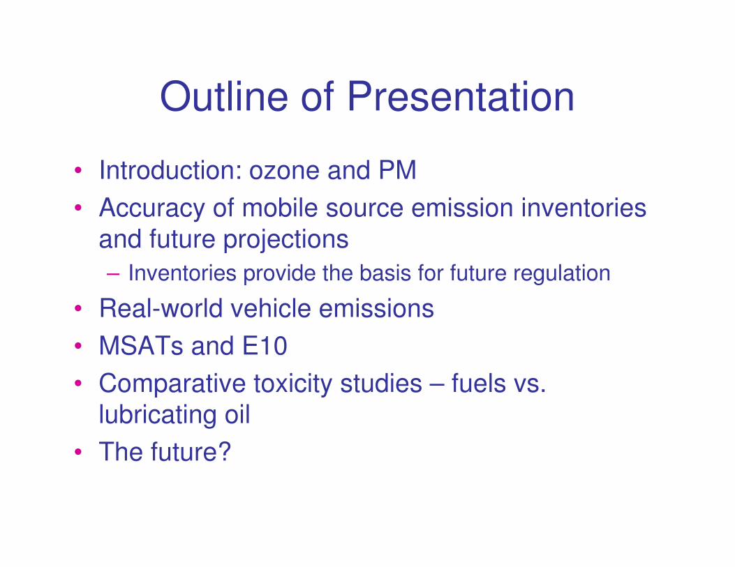
Nonattainment Areas for Ozone and PM2.5

(2004) No. of Counties

with Monitors

exceeding the

NAAQS

• CO 0

• Lead 1

• SO2 0

• NO2 0

• PM10 12

• PM2.5 82

• O3 297

“Ozone and PM Are Our Highest Priority” – from “Air Quality Management in the

21st Century,” John Bachmann, EPA, October 18, 2005

From: “Latest Findings on National Air Quality: 2001 Status and Trends”

Evolution of California Auto Controls(Implementation: 1963 – 1993)

0

2

4

6

8

10

12

14

1963

1965

1967

1969

1971

1973

1975

1977

1979

1981

1983

1985

1987

1989

1991

1993

g/m

ile N

MV

OC

+ N

Ox

Positive Crankcase Ventilation

Exhaust Standards

EGR

Oxidation Catalyst

Three Way CatalystOn-Board Computer

Advanced ComputerFuel Injection

O2 Sensor

Phase 1 Gasoline

Ref: A. Lloyd, 13th CRC On-Road Vehicle Emissions Workshop, San Diego, CA, April 2003

0

0.1

0.2

0.3

0.4

0.5

0.6

0.7

1994

1995

1996

1997

1998

1999

2000

2001

2002

2003

2004

2005

2006

2007

2008

2009

2010

g/m

ile N

MV

OC

+ N

Ox

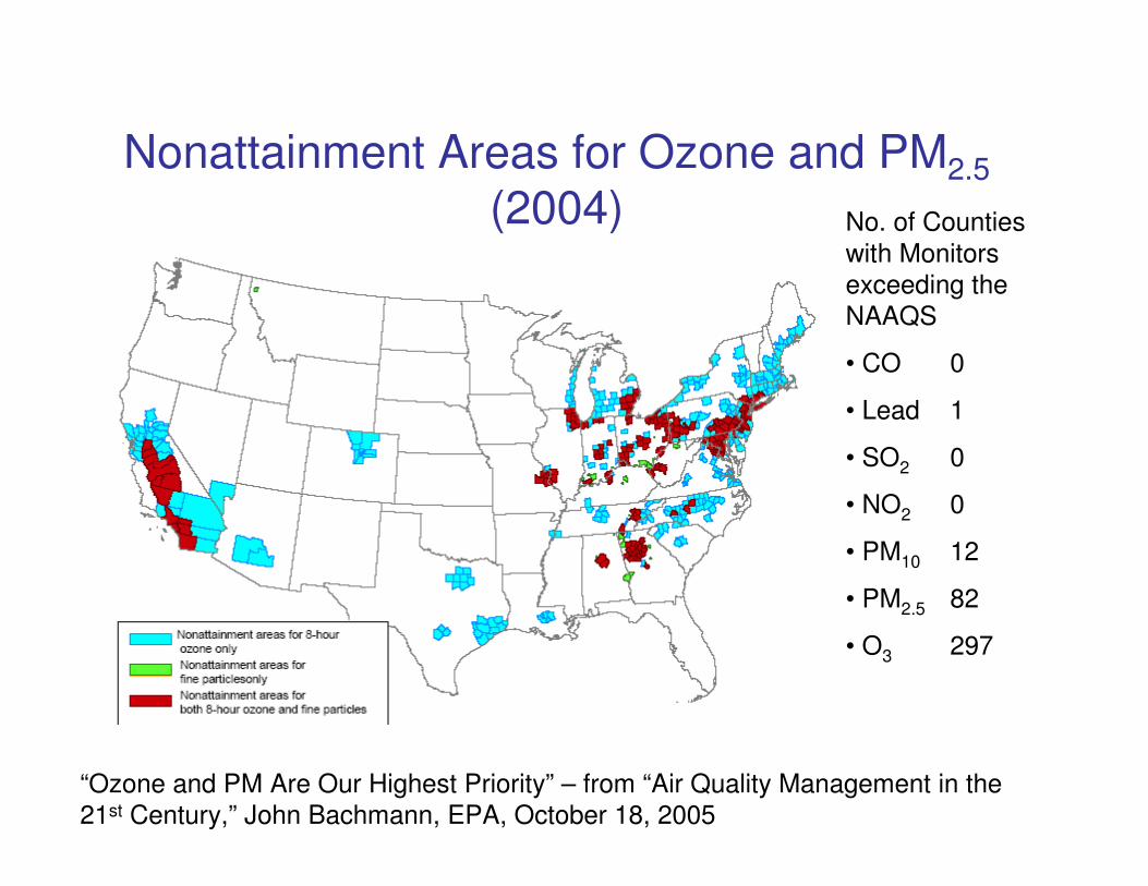
Evolution of California Auto Controls(Implementation: 1994 – 2010)

Low Emission Vehicle I

Phase 2 Gasoline

Low Emission Vehicle II

Ref: A. Lloyd, 13th CRC On-Road Vehicle Emissions Workshop, San Diego, CA, April 2003

Ref: C.E. Freese, 13th DEER Conference, Detroit MI, August 2007

Ozone trends in the South Coast Air Basin 1973 through 2006

0

0 .1

0 .2

0 .3

0 .4

0 .5

0 .6

7 3 7 4 7 5 7 6 7 7 7 8 7 9 8 0 8 1 8 2 8 3 8 4 8 5 8 6 8 7 8 8 8 9 9 0 9 1 9 2 9 3 9 4 9 5 9 6 9 7 9 8 9 9 0 0 0 1 0 2 0 3 0 4 0 5 0 6

1 -h r M a x 1 -h r 3 y r 4 th H i 8 -h r M a x 8 -h r 3 y r A ve 4 th H i

The California Air Resources Board says that “Cleaner-burning gasoline reduces smog-forming

emissions from motor vehicles by 15 percent.” (http://www.arb.ca.gov/fuels/gasoline/cbgupdat.htm).

In which year was CBG introduced?

4th Maximum 8-hr. Ozone

Denver Area

0.000

0.010

0.020

0.030

0.040

0.050

0.060

0.070

0.080

0.090

0.100

1993

1994

1995

1996

1997

1998

1999

2000

2001

2002

2003

2004

2005

2006

2007

*4th

Maxim

um

8-H

r. O

zo

ne (

pp

m)

NREL R. Flats-N Chatfield FC-W

Mobile Sources Largest Contributor

to Urban Air Quality

• Why are we having so much difficulty in reducing ambient ozone (and PM) levels?

• New vehicle certification standards have reduced emissions as much as 99%– Is it impossible to reduce ambient ozone (and

PM) levels?

– Are we not doing enough of everything?, or

– Are our control programs not doing enough of the right thing?

Emission Inventories for

PM, CO, VOC

Provide Basis for Control Strategies

Projected Contributions of Mobile

Sources to Los Angeles Air Quality

• “It is apparent that by 1980, motor vehicles will not be the major source of hydrocarbons and oxides of nitrogen, and greater emphasis will have to be placed on emissions from nonvehicular sources.” – Air Pollution Control in California, 1971 Annual Report, page 34.

• “Contribution to VOC by mobile sources is reduced due to the CARB programs. On the contrary, area sources become major contributors to VOC emissions (from 28% in 1997 to 36% in 2010).” 2003 South Coast AQMD, Appendix 3, page III-2-15.

• “However, contribution to VOC by mobile sources is reduced due toCARB regulations over time. Area sources become major contributors to VOC emissions (from 27 percent in 2002 to 42 percent in 2020).”, Draft 2007 South Coast AQMP, Appendix III, page III-2-14.

“Forecasting is difficult, especially when it involves the future.” Quote attributed

to C. Stengel or Y. Berra, depending on the source.

Nationwide PM2.5 Emission Inventory, 2002

www.epa.gov/ttn/chief/trends/index.html#tables

0

500

1,000

1,500

2,000

2,500

Fuel C

ombus

tion

Indu

stria

l Pro

cess

es

Misc

ella

neous

Fugiti

ve D

ust

Mob

ile, G

asolin

e

Mob

ile, D

iese

l

Kil

oto

ns/

year

Phoenix PM2.5 Comparison

5%

17%

16%

35%

14%

13%

Gasoline Exhaust Diesel Exhaust Crustal/Soil Vegetative Burning Secondary Sulfates Secondary Nitrates

Emission Inventory Ambient Data/Receptor Modeling

28%

14%

19%

8%

16%

15%

Refs: Emission Inventory, EPA OAQPS, 1997; Ambient Results: Lewis et al., JAWMA, 2003

0

4000

8000

12000

16000

80 82 84 86 88 90 92 94 96 98 00 02 04

Year

To

ns/D

ay

0

25

50

75

100

Days >

8-h

r F

ed

Std

Tons/Day (current est.) 1999 Almanac

2006 Almanac Days >8-hr Fed Std

Mobile Source Emission Inventory Reality Check:

South Coast Air Basin CO Trends Ambient vs. Inventory, 1980-2005

2.4x

1987 SCAQS Tunnel Study: On-road mobile emissions were 2.7 and 3.8 times

higher for CO and NMHC than EMFAC7C model predictions

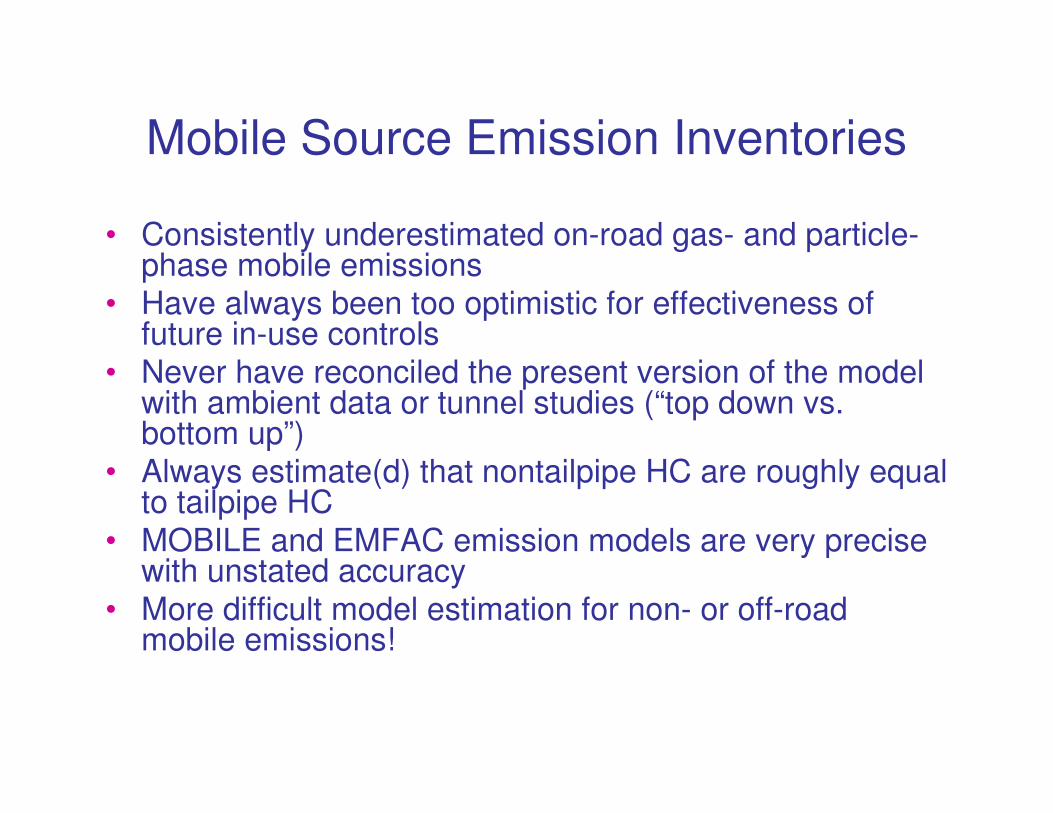
Mobile Source Emission Inventories

• Consistently underestimated on-road gas- and particle-phase mobile emissions

• Have always been too optimistic for effectiveness of future in-use controls

• Never have reconciled the present version of the model with ambient data or tunnel studies (“top down vs. bottom up”)

• Always estimate(d) that nontailpipe HC are roughly equal to tailpipe HC

• MOBILE and EMFAC emission models are very precise with unstated accuracy

• More difficult model estimation for non- or off-road mobile emissions!

Real-World Vehicle Emissions

Nationwide On-

Road Idle HC

Emissions

EPA’s 1985 National

Tampering Survey

6498 vehicles

Ref: Lawson et al. 1996

On average, fleet emissions increase as vehicles age; mean fleet emissions driven by high emitters; median vehicle is clean

Most new cars are clean; a few new vehicles are dirty; most old cars are “clean”

New vehicles irrelevant to air quality

1983 (

25)

1985

1987

1989

1991

1993

1995

1997

1999

2001 (

1113)

2003

0.000

0.050

0.100

0.150

0.200

0.250

Average HC

Emissions, %

Model Year

Cleanest Quintile

2nd Cleanest

Marginal

Dirtier

Dirtiest Quintile

Remote Sensing HC Emissions by Quintile

Speer Blvd./I-25 (Denver)

1983 (

25)

1985

1987

1989

1991

1993

1995

1997

1999

2001 (

1113)

2003

0.0

1.0

2.0

3.0

4.0

5.0

6.0

% of Total HC

Model Year

Cleanest Quintile

2nd Cleanest

Marginal

Dirtier

Dirtiest Quintile

Dec. 3, 5, 6, 2002

10,015 Measurements

Ref: http://www.feat.biochem.du.edu

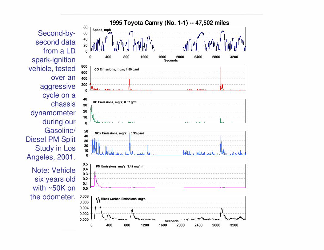
1995 Toyota Camry (No. 1-1) -- 47,502 miles

0

20

40

60

80

0 400 800 1200 1600 2000 2400 2800 3200Seconds

Speed, mph

0

200

400

600

800CO Emissions, mg/s; 1.80 g/mi

0

10

20

30

40HC Emissions, mg/s; 0.07 g/mi

0

10

20

30

40

50 NOx Emissions, mg/s; 0.35 g/mi

0.0

0.1

0.2

0.3

0.4

0.5 PM Emissions, mg/s; 3.42 mg/mi

0.000

0.002

0.004

0.006

0.008

0 400 800 1200 1600 2000 2400 2800 3200Seconds

Black Carbon Emissions, mg/s

Speed, mph

Second-by-

second data

from a LD

spark-ignition

vehicle, tested

over an

aggressive

cycle on a

chassis

dynamometer

during our

Gasoline/

Diesel PM Split

Study in Los

Angeles, 2001.

Note: Vehicle

six years old

with ~50K on

the odometer.

0

200

400

600

800

Seconds

Cold Phase Warm Phase

CO Emissions, mg/sec; 2.28 g/mi (cold); 1.44 g/mi (warm)

0

10

20

30

40

Seconds


HC Emissions, mg/sec; 0.16 g/mi (cold); 0.01 g/mi (warm)

01020304050

Seconds


NOx Emissions, mg/sec; 0.46 g/mi (cold); 0.26 g/mi (warm)

0.0

0.1

0.2

0.3

0.4

Seconds


PM Emissions, mg/sec; 7.7 mg/mi (cold); 0.2 mg/mi (warm)

0.0000.0020.0040.0060.008

0 200 400 600 800 1000 1200 1400Seconds


BC Emissions, mg/sec

1995 Toyota Camry (No. 1-1) -- 47,502 miles

0

20

40

60

80

0 200 400 600 800 1000 1200 1400Seconds

Speed, mph

0.00

0.10

0.20

0.30

0.40

0.50

0.60

Em

issio

n R

ate

, m

g/m

i

Benz(a)anthracene Chrysene Benzo(b+j+k)fluoranthene Benzo(a)pyrene Indeno[123-cd]pyrene Dibenzo(ah+ac)anthracene

Spark Ignition Emissions of PAH (POM) Listed as MSATs

0.000

0.001

0.002

0.003

0.004

0.005

0.006

SI Vehicle Profile

Fra

ctio

n o

f P

M M

ass

CW

CW

CW

CW

SMOKERSNewer Vehicles

Older VehiclesCW

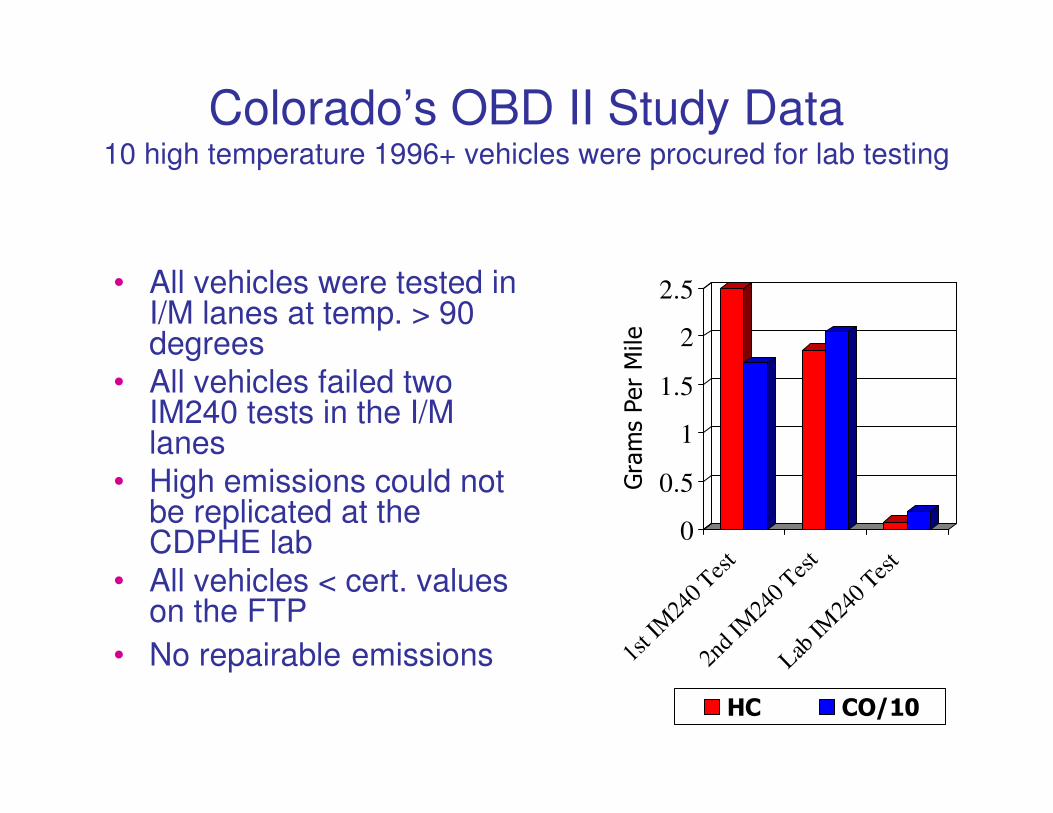
Colorado’s OBD II Study Data10 high temperature 1996+ vehicles were procured for lab testing

• All vehicles were tested in I/M lanes at temp. > 90 degrees

• All vehicles failed two IM240 tests in the I/M lanes

• High emissions could not be replicated at the CDPHE lab

• All vehicles < cert. values on the FTP

• No repairable emissions

0

0.5

1

1.5

2

2.5

Grams Per Mile

1st I

M24

0 Tes

t

2nd

IM24

0 Tes

t

Lab IM

240

Test

HC CO/10

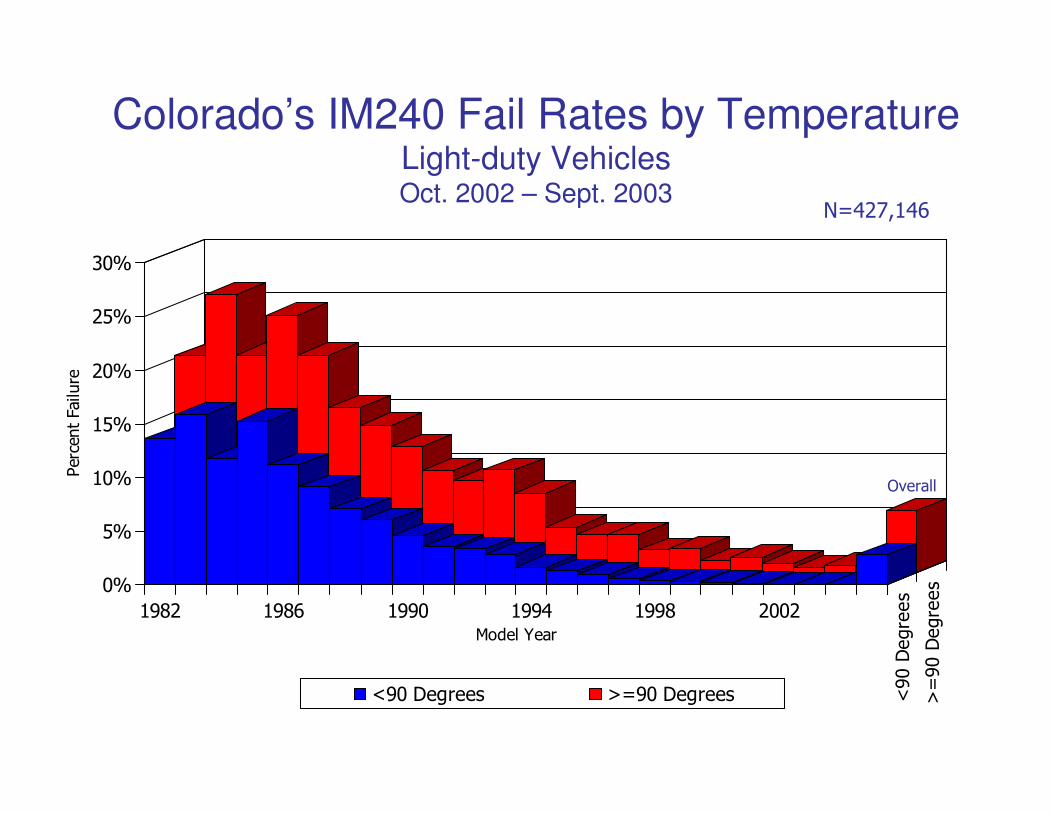
0%

5%

10%

15%

20%

25%

30%

Percent Failure

1982 1986 1990 1994 1998 2002

<90 Degrees

>=90 Degrees

Model Year

<90 Degrees >=90 Degrees

Colorado’s IM240 Fail Rates by TemperatureLight-duty VehiclesOct. 2002 – Sept. 2003

N=427,146

Overall

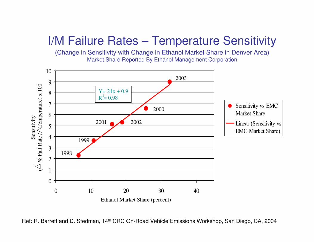
I/M Failure Rates – Temperature Sensitivity(Change in Sensitivity with Change in Ethanol Market Share in Denver Area)

Market Share Reported By Ethanol Management Corporation

0

1

2

3

4

5

6

7

8

9

10

0 10 20 30 40

Sensitivity vs EMC

Market Share

Linear (Sensitivity vs

EMC Market Share)

Ethanol Market Share (percent)

Sen

siti

vit

y

( %

Fai

l R

ate

/ T

emp

erat

ure

) x

100

1999

1998

2001 2002

2000

2003

Y= 24x + 0.9

R = 0.982

Ref: R. Barrett and D. Stedman, 14th CRC On-Road Vehicle Emissions Workshop, San Diego, CA, 2004

DOE’s Comparative Toxicity Studies

Comparative Toxicity of Particulate and Semi-Volatile Organic

Emissions from Normal and High-Emitting Gasoline, Diesel and

Compressed Natural Gas Engines

1. PM and vapor-phase SVOCs from vehicles on chassis dynamometers (SwRI)

Gasoline G (normal emitter) 5 1982-1996 automobiles, 35 – 190K mi

BG (black smoker) 1976 malfunctioning pickup, 199K mi

WG (white smoker) 1990 malfunctioning automobile, 185K mi

Diesel D (normal emitter) 3 1998-2000 automobiles & pickup, 7- 48K mi

HD (high emitter) 1991 malfunctioning pickup, 27K mi

CNG NT (new technology) 2002 with oxidation catalyst, 216 mi

(transit buses) NE (normal emitter) 1997, no after-treatment, 134K mi

HE (high emitter) 1992, retired with 250K miles

2. Chemistry analyzed in detail (DRI)

3. Instilled combined PM+SVOC (in original mass ratios) into rat lungs, and

measured inflammation at 24 hr by bronchoalveolar lavage (LRRI)

4. Compared inflammatory potential (average of 5 variables) per unit of mass (LRRI)

5. Used multivariate analysis (PCA-PLS) to identify components co-varying most

closely with toxicity (LRRI)Seagrave et al., Toxicol. Sci. 70:212, 2002McDonald et al., Environ. Health Perspect. 112:1527, 2004

Zielinska et al., J. Air Waste Man. Assoc. 54:1138, 2004

Seagrave et al., Toxicol. Sci. 87:232, 2005

0

0.5

1

1.5

2

2.5

3

3.5

G BG WG D HD NT NE HE

----- Gasoline ------ -- Diesel -- --------- CNG --------

----------------------------------------------------------------------

Bacterial Mutagenicity

Per Unit of Mass,

Relative to Normal

Gasoline

(Salmonella T-98)

Comparison of Bacterial Mutagenicity

•••• Per unit of PM+SVOC mass, normal gasoline and diesel had similar

mutagenicity

•••• Masses from normal and high emitting CNG buses were the most

mutagenic

0

1

2

3

4

5

6

7

G BG WG D HD NT NE HE

-----------------------------------------------------

Inflammatory Potential

Per Unit of Mass,

Relative to Normal

Gasoline

----- Gasoline ------ -- Diesel -- --------- CNG --------

Comparison of Lung Inflammatory Potential

•••• Per unit of PM+SVOC mass, normal gasoline and diesel had similar potency,

CNG had lower potency

•••• Mass from high-emitting gasoline & diesel vehicles was more toxic

Observed

Predicted

2.01.51.00.50.0

2.0

1.5

1.0

0.5

0.0

High EmitNew Tech Norm Emit

D30G30

HD

D

WG

BG

G

Obseved vs Fitted Inflam. Histopatholgy

....

WG

••••

HD

••••BG

D

••••

G

NT HE NE ••••

•••• ••••

Multivariate Analysis Implicated Lubricating Oil

•••• Models to predict relative responses based on composition were optimized

•••• Composition variables were ranked by their influence on the models

0.00

0.20

0.40

0.60

0.80

1.00

1.20

1.40

1.60

S-18H-7

H-12

O2TC

S-4H-6

E2TC

H-5S-9S-5

H-16

S-10

S-1H-3

H-15

S-14

S-3H-8S-8

S-20

S-19

S-17

S-7

S-11H-4EC

S-12

S-2

H-11

H-10

H-9

PartOC

S-13

H-2H-1

S-16

H-14

H-13

S-6

SO4

E3TC

EarthMet

NonMetTC

PM

SVOC

O1TC

4ringPAH

Metalloi

3AMet

O3TC

5ringPAH

O4TC

NO3

E1TC

PMPAH

>5ringPA

TransMet

TotPAH

SVOCPAH

3ringPAH

4AMet

2ringPAH

S-15

NH4

OxyPAH

NitroPAH

OPTC

VIP

•••• 27 of the top 30 variables were hopanes or steranes, markers of

crankcase lube oil

Example: model fitted to histopathology scores

Light-Duty Vehicle Emissions• Light-duty vehicles have been built “clean” since 1982• High-emitter “wall” has progressed forward with passage of time;

fleet turnover has somewhat reduced the number of high emitters,but a small fraction (~5%) produces over half the on-road tailpipe emissions. The U.S. will not attain the national ambient air quality standards until the high emitter problem is solved. Adopting California’s LEV standards does little, if anything, to improve air quality.

• I/M programs, depending upon configuration, have done much less to reduce emissions than the models predict. In some locations, there has been no empirically observed benefit from I/M programs

• High emitters are high emitters regardless of the fuel used (i.e., treating the symptom rather than the problem)

• Oxygen in gasoline (lower level E-XX blends) produces increased permeation (nontailpipe) emissions of VOC relative to non-EtOHcontaining gasoline

• Increased carbonyl emissions (formaldehyde and acetaldehyde –and likely many more oxygenated species) are produced by oxygenated gasoline

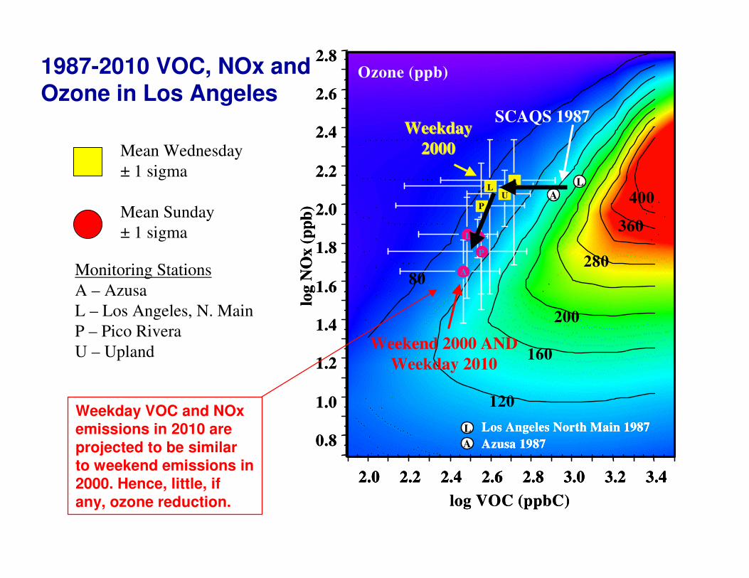
Monitoring Stations

A – Azusa

L – Los Angeles, N. Main

P – Pico Rivera

U – Upland

400

360

120

160

200

28080

2.0 2.2 2.4 2.6 2.8 3.0 3.2 3.4

2.8

2.6

2.4

2.2

2.0

1.8

1.6

1.4

1.2

1.0

0.8

log N

Ox (

pp

b)

log VOC (ppbC)

Ozone (ppb)

400

360

120

160

200

28080

2.0 2.2 2.4 2.6 2.8 3.0 3.2 3.42.0 2.2 2.4 2.6 2.8 3.0 3.2 3.4

2.8

2.6

2.4

2.2

2.0

1.8

1.6

1.4

1.2

1.0

0.8

log N

Ox (

pp

b)

log VOC (ppbC)

Ozone (ppb)

P

LU

A

A

L U

P

Los Angeles North Main 1987

Azusa 1987

L

A

A

L

P

LU

A

A

L U

P


Azusa 1987

L

A


Azusa 1987

L

A

A

L

Mean Wednesday

± 1 sigma

Mean Sunday

± 1 sigma

1987-2010 VOC, NOx and Ozone in Los Angeles

Weekday VOC and NOx

emissions in 2010 are

projected to be similar

to weekend emissions in

2000. Hence, little, if

any, ozone reduction.

SCAQS 1987

Weekend 2000 AND

Weekday 2010

WeekdayWeekday

20002000

Questions?

Documents

Fuels and Exposure – Is It Really the Fuels?/media/Files/Activity Files... · Fuels and Exposure – Is It Really the Fuels? ... • More difficult model estimation for non- or