arX

iv:1

204.

1521

v2 [

hep-

th]

12

Jun

2013

Fubini instantons in curved space

Bum-Hoon Leea,b∗, Wonwoo Leeb†, Changheon Ohc‡, Daeho Roa§,

and Dong-han Yeomb,d¶

aDepartment of Physics and BK21 Division, Sogang University, Seoul 121-742, Korea

bCenter for Quantum Spacetime, Sogang University, Seoul 121-742, Korea

cMeerecompany, Gyeonggi-do 445-938, Korea

dYukawa Institute for Theoretical Physics, Kyoto University, Kyoto 606-8502, Japan

September 17, 2018

Abstract

We study Fubini instantons of a self-gravitating scalar field. The Fubini instantondescribes the decay of a vacuum state under tunneling instead of rolling in the presenceof a tachyonic potential. The tunneling occurs from the maximum of the potential, whichis a vacuum state, to any arbitrary state, belonging to the tunneling without any barrier.We consider two different types of the tachyonic potential. One has only a quartic term.The other has both the quartic and quadratic terms. We show that, there exist severalkinds of new O(4)-symmetric Fubini instanton solution, which are possible only if gravityis taken into account. One type of them has the structure with Z2 symmetry. This type ofthe solution is possible only in the de Sitter background. We discuss on the interpretationof the solutions with Z2 symmetry.

PACS numbers: 04.62.+v, 98.80.Cq

∗bhl@sogang.ac.kr

†warrior@sogang.ac.kr

‡choh0423@gmail.com

§dhro@sogang.ac.kr

¶innocent.yeom@gmail.com

1

1 Introduction

The very first picture of an inflationary multiverse scenario was proposed in Ref. [1], in which itwould seem that the author wanted to suggest a universe without the cosmological singularityproblem using an interesting feature of self-reproducting or regenerating exponential expansionof the universe. A major development in this scenario was triggered by the discovery of theeternal inflationary scenario [2–5] and a paradigm for string theory landscape [6,7]. The eternalinflation is related to the expanding false vacuum solution with a positive cosmological constant,which in turn means that the inflation is eternal into the future. If the theory has multipleminima then the false vacuum state decays into the true vacuum state, i.e. the phase transitionproceeded via the nucleation of a vacuum bubble. In this scenario the universe is situated withinsome bubble called a pocket universe [4] having a certain value of the cosmological constant andthe whole universes are referred to as multiverse. The description of self-reproduction includingtunneling process and random walk was combined into a scenario called recycling universe [8].These scenarios seem to provide an escape from the question of the initial conditions of theuniverse, i.e. it seems to be eternal into the past. Unfortunately, inflationary spacetimescannot be made complete in the past direction [9], even though the universe is eternal intothe future. There are still interesting arguments on the beginning of the universe [10]. Thestring theory landscape is a setting that involves a huge number of different metastable andstable vacua [11,12], originated from different choices of Calabi-Yau manifolds and generalizedmagnetic fluxes. The huge number of different vacua can be approximated by the potential ofa scalar field. The important thing is the fact that, once the de Sitter vacuum can exist, theinflationary expansion is eternal into the future and has the possibility of self-reproduction.

On the other hand, there are theories of gauged d = 4, N = 8 supergravity having deSitter(dS) solution, in which all SUSYs are spontaneously broken. It is well known that thedS solution corresponds to a M/sting theory solution with a non-compact 7- or 6-dimensionalinternal space, in which a small value of the cosmological constant stems from the 4-form flux.The simplest representative of these kind of theories has a tachyonic potential with the dSmaxima [13–15]. The potential in the vicinity of the maximum reduces to a form having aquadratic term, that is not metastable but unstable. However, according to some authors, thetime for collapse giving rise to the tachyonic potential can be much greater than the age of theuniverse for anthropic reasoning. If the curvature radius of the potential in the vicinity of themaximum is greater than that used in the above theory, then that will be all together differentstory. The supergravity analogue of the tachyonic potential could be constructed also by usingan exact supergravity solution representing the Dp-Dp system [16].

From the above scenarios, the study of the possibility of the tunneling process for thepotential with stable and metastable vacua, or even tachyonic behavior has acquired renewedinterest. In the present paper, we will study the tunneling process under a simple tachyonicpotential governed by a quartic term both without the quadratic term and with the term as atoy model. To obtain the general solution including the effect of the backreaction, we solve thecoupled equations for the gravity and the scalar field simultaneously. Although the model has

2

a tachyonic potential, it might still be an useful example to show how the tunneling processoccurs in various shapes of the potential provided by the above scenarios.

A quantum particle can tunnel through a finite potential barrier via the so-called barrierpenetration. This process can be described by the Euclidean solution obeying appropriateboundary conditions. There exist two kinds of Euclidean solutions describing quantum tunnel-ing phenomena. One corresponds to an instanton solution representing a stable pseudoparticleconfiguration characterized by the existence of a nontrivial topological charge. It does notchange even if we continuously deform the field, as long as the boundary conditions remain thesame. The instanton solution corresponds to the minimum of the Euclidean action to pass fromthe initial to final state [17]. The solution, in case of a double well potential, describes a generalshift in the ground state energy of the classical vacuum due to the presence of an additionalpotential well, then lifting the so-called classical degeneracy. The other is a bounce solutionrepresenting an unstable nontopological configuration that corresponds to a saddle point ratherthan a minimum of the Euclidean action. The second derivative of the Euclidean action aroundthe bounce has one negative eigenvalue which leads to the imaginary part of the energy. Theexistence of the negative eigenvalue implies that the vacuum state is unstable, i.e. the statedecays into other states [18].

The Euclidean solutions can also mediate phase transitions. The phase transition describesthe sudden change of a physical system from one state to another. The transition are of twodifferent types transition accompanied by temperature or zero temperature. The competitionbetween the entropy and the energy terms in the thermodynamic potential cause thermal phasetransitions in which dynamics is irrelevant. In the modern classification scheme, thermal phasetransitions are divided into two broad categories either with a discontinuous jump in the first-order derivatives of the free energy or without it. A first-order phase transition is characterizedby the discontinuity in the first derivative of the free energy and is associated with the existenceof latent heat, whereas a nth-order phase transition is characterized by the continuity in thefirst derivative while there is a discontinuity in the nth-order derivative. A quantum phasetransition describes a transition between different phases by quantum fluctuation, which occursat zero temperature, unlike the case of a thermal phase transition which is governed by athermal fluctuation [19].

To simplify things, we consider an asymmetric double well potential to distinguish twodifferent phase transitions at zero temperature. If the initial state is the metastable vacuumstate and the tunneling occurs from that state to the other vacuum state, then the transitioncorresponds to a tunneling process [20–25]. On the other hand, if the initial state is the localmaxima of the potential and the field is rolling down to one vacuum state continuously ratherthan any discontinuous jump, then the transition corresponds to the rolling. However, onemore channel exists as tunneling and that corresponds to the one without a barrier. In thiskind of transition, the initial state on the top of a potential can tunnel to the other staterather than rolling down the potential [26–28, 30]. There are two different kind of transitionsin this case. One is the tunneling without a barrier representing the tunneling from the localmaximum of the potential to the vacuum state [28–31]. Recently, an analytic study on this

3

type of solution was performed in [31]. The other is a tunneling without a barrier representingthe tunneling from the maximum of the potential to any arbitrary state. This case correspondsto the Fubini instanton [26, 27], where the tachyonic potential is employed. Can we describethe rolling corresponding to the transition between the initial metastable vacuum state and theother final vacuum state? This may look similar to a superfluid motion by the liquid helium.Although to establish the phase transition corresponding to the superfluid motion is itself avery challenging problem, we concentrate on the Fubini instantons in this work.

The Fubini instanton [26, 27] describes the decay of a vacuum state by the quantum phasetransition instead of rolling down the tachyonic potential consisted of a quartic term only. Onthe other hand, one can consider a tachyonic potential consisted of a quadratic term only, thepoint Φ = 0 is unstable. A small perturbation will cause it to roll down the hill of the potential.Originally, it was Fubini who introduced a fundamental scale of hadron phenomena by means ofthe dilatation noninvariant vacuum state in the framework of a scale invariant Lagrangian fieldtheory [26]. However, the solution is a one-parameter family of instanton solutions representinga tunneling without a barrier as an interpolating solution from the maximum of the potentialto any arbitrary state. The instanton solution was studied in a conformally invariant model,i.e. a fixed background was used and the effect of the backreaction by instantons was neglected[32–34]. This is a good approximation, when the variation of the potential during the transitionis much smaller than the maximum of the potential. The instanton has gained much interestnow-a-days in the context of anti-de Sitter(AdS)/conformal field theory correspondence [35,36].

The paper is organized as follows: In Sec. 2, we review the Fubini instanton in the absence ofgravity. We present numerical solutions including the Euclidean energy density as an exampleand analyze the structure of the solution in the theory with a potential having only the quarticself-interaction term. We stress the fact that there is no such solutions with the potentialcontaining both the quartic and the quadratic terms. In Sec. 3, we show that the instantonsolutions exist in the curved space. We perform a numerical study to solve the coupled equationsfor the gravity and the scalar field simultaneously. We show that there exist numerical solutionswithout oscillation in the initial AdS space in the potential with only the quartic term. Wealso show that there exist numerical solutions in the potential both with the quartic and thequadratic terms irrespective of the value of the cosmological constant, which is possible onlywhen the gravity is switched on. In order to estimate the decay rate of the background state,we compute the action difference between that of the solution and the background obtained bynumerical means. We present an oscillating numerical solutions in the potential with only thequartic term with various values of the cosmological constant. One type of these solutions hasthe structure with Z2 symmetry. We will discuss on the interpretation of the solutions withZ2 symmetry in the final Section. We analyze the behavior of the solutions using the phasediagram method. In Sec. 4, to observe the dynamics of the solutions, we briefly sketch thecausal structures of the solutions in the Lorentzian spacetime. Finally in Sec. 5, we summarizeand discuss our results.

4

2 Fubini instanton in the absence of gravity

One can consider the following action in the absence of gravity

S =

∫

M

√−gd4x

[

−1

2∇αΦ∇αΦ− U(Φ)

]

, (1)

where g = det ηµν , ηµν = diag(−1, 1, 1, 1) is the Minkowski metric, and the tachyonic potentialhas a quartic self-interaction term and also a quadratic term as follows:

U(Φ) = −λ

4Φ4 +

m2

2Φ2 + Uo, (2)

where m2 > 0 and λ > 0. The plots of potentials (a) without the quadratic term and (b) withthe quadratic term are shown in Fig. 1. The potential has a metastable vacuum state at Φ = 0and no other stationary state in Fig. 1(a), while Fig. 1(b) illustrates that the potential has alocal minimum at Φ = 0 and two maxima [27, 37, 38]. In both the cases, the potential is notbounded from below.

Before going to the tunneling problem in four dimensions, we briefly describe the problemin one dimension. One can consider the simplest quantum tunneling problem in one dimension.Quantum field theory in one dimension is nothing but ordinary quantum mechanics. In caseof m2 = 0, the amplitude for transmission obeys the WKB formula in the semiclassical ap-proximation, in which Φ± = ±(4Uo

λ)1/4 are the classical turning points. On the other hand, the

double-hump potential with m2 > 0 and Uo = 0 can be considered as an inverted double-wellpotential for a bounce solution representing the tunneling from Φ = 0 to Φ± = ±m

√

2/λ. The

solution is given by Φs(τ) = ±m√

2/λsech[m(τ − τo)], where τo is an integration constant. Thebounce solutions can be easily understood in the Euclidean space. The particle can only reachthe point Φ = 0 at τ = ±∞ and it bounces off Φ± = ±m

√

2/λ at τ = 0 with a vanishingvelocity [39].

We now turn to the tunneling problem in four dimensions. It is an well-known fact thatthe massless theory has an instanton [26]. Actually, the instanton corresponds to the bouncesolution representing the decay of the background vacuum state. The equation of motion withO(4) symmetry, obtained by varying the Euclidean action, is then;

d2Φ

dη2+

3

η

dΦ

dη= −d(−U)

dΦ, (3)

where η(=√τ 2 + x2) plays the role of the evolution parameter in Euclidean space and the

second term in the left-hand side plays the role of a damping term. The boundary conditionsare

dΦ

dη

∣

∣

∣

η=0= 0 and Φ|η=∞ = 0 . (4)

The particle in the classical mechanics problem starts at Φ = Φo with zero velocity in theinverted potential, and stops at Φ|η=∞ = 0 without any oscillation.

5

(b)(b)

Uo

U

Uo

U(a)

Figure 1: Potentials for the case of (a) Fubini instantons and (b) generalized Fubini instantons.

For the potential with m2 = 0, the analytic solution of the Fubini instanton has the form

Φ(η) =

√

8

λ

b

η2 + b2, (5)

where η is the radial length in the Euclidean space, b is any arbitrary length scale whichcharacterizes the size of the instanton and is related to the initial value Φo. In addition, the

value of the scalar field of the center of the solution depends on b as Φ(0) =√

8λ1b. This solution

was used in the related perturbation theory [40].

The characteristic behavior of the analytic solution is ploted in Fig. 2 in terms of the valueof the parameter b. We take λ = 1 for all the cases. The solid line denotes the solution withb = 1, the dashed line with b = 3, and the dotted line with b = 5. The corresponding Euclideanaction is given by

SE =32π2b2

λ

∫ ∞

0

η5(1− b2

η2)

(η2 + b2)4dη =

8π2

3λ, (6)

where the action does not depend on the parameter b due to the consequence of the conformalinvariance of the potential and we take that value to be Uo = 0. The action has the same valueirrespective of the starting point Φo. In other words, the tunneling from the maximum of thepotential to any arbitrary state always happens with same probability.

The numerical solutions for Φ and Φ′ and the Euclidean energy including the density varia-tion with η are as shown in Fig. 3. Figure 3(a) illustrates the numerical solution for Φ, in whichthe initial value set as Φo = −1 and the solution asymptotically approaches the value Φ = 0.Figure 3(b) illustrates Φ′ with respect to η. There is a peak of Φ′ near η = 2.31. Figure 3(c)depicts the volume energy density, when the density has got the form ξ = [1

2Φ′2+U ]. The lower

6

0 2 4 6 8 100.0

0.5

1.0

1.5

2.0

2.5 b=1 b=3 b=5

Figure 2: The analytic solution of the Fubini instanton in absence of gravity.

right box in the same figure shows the magnification of the small region clearly representing theexistence of a smooth hill. The smooth peak of the volume energy density exists at η = 5.17.There is a disagreement between the location of the peak for the energy density and that forΦ′. It clearly reveals the fact that the position with the maximum value for Φ′ is still not thesame as the maximum of the energy density due to non-trivial contribution coming from thepotential, U = −λ

4Φ4. Figure 3(d) shows the Euclidean energy Eξ for each slice of constant η.

The Euclidean energy signifies the value of energy after the full integration of variables exceptfor η in the present work, Eξ = 2π2η3ξ. There are one minimum and one maximum point forEξ. The location of the minimum of Eξ is around η = 2.31, whereas that of the maximumis near η = 6.93. Ironically, the location of the minimum of Eξ coincides with that of themaximum of Φ′. These solutions can be considered as a ball consisting of only a thick wallexcept for one point at the center of the solution with a lower arbitrary state than the outervacuum state unlike a vacuum bubble that consists of an inside part with a lower vacuum stateand a wall.

For a theory with m2 > 0, the conformal invariance is broken and any solution with a finiteaction is forbidden by scaling argument. In other worlds, the particle can not have enoughenergy to reach the hill overcome the barrier near Φ = 0 since the damping term has got a largevalue due to a large value of Φ′ near the initial point [41].

3 Fubini instantons of a self-gravitating scalar field

Let us consider the following action:

S =

∫

M

√−gd4x

[

R

2κ− 1

2∇αΦ∇αΦ− U(Φ)

]

+

∮

∂M

√−hd3x

K −Ko

κ, (7)

7

0 20 40-8

0

8

(d)

0 20 40

-0.1

0.0

5 10

0.000

0.002

(c)

0 20 400.00

0.09

0.18(b)

'

0 20 40-1.0

-0.5

0.0

(a)

Figure 3: (a) The numerical solution for Φ in the case of m2 = 0, (b) the variation of Φ′ with respect to η,(c) the energy density ξ and (d) the Euclidean energy Eξ evaluated at constant η.

where g = det gµν , κ ≡ 8πG, R denotes the scalar curvature of the spacetime M, h is theinduced boundary metric, K and Ko are the traces of the extrinsic curvatures of ∂M forthe metric gµν and ηµν , respectively. The second term on the right-hand side is the boundaryterm [42]. It is necessary to have a well-posed variational problem including the Einstein-Hilbertterm. Here we adopt the notations and sign conventions of Misner, Thorne and Wheeler [43].

We study the creation process of Fubini instantons in curved spacetime. In the first place,we consider the massless case, and then we will also consider generalized Fubini instantons, theso-called massive case (see the form of the potential in Eq. (2)). The cosmological constant isgiven by Λ = κU0, such that background space will be dS, flat or AdS depending on the signsof U0.

In order to solve the coupled equations, we assume an O(4) symmetry for the geometry andthe scalar field similar to Ref. [22]

ds2 = dη2 + ρ2(η)[

dχ2 + sin2 χ(

dθ2 + sin2 θdφ2)]

. (8)

8

And then, Φ and ρ depends only on η, and the Euclidean equation can be written respectivelyas follows:

Φ′′ +3ρ′

ρΦ′ =

dU

dΦand ρ′′ = −κ

3ρ(Φ′2 + U) , (9)

and the Hamiltonian constraint is then given by

ρ′2 − 1− κρ2

3

(

1

2Φ′2 − U

)

= 0 . (10)

In order to yield a meaningful solution, the constraint requires a delicate balance among all thedifferent terms. Otherwise the solution can yield qualitatively incorrect behavior [44].

To solve the Eqs. (9), we have to impose suitable boundary conditions. When the gravity

is switched off, boundary conditions for the Fubini instanton are dΦdη

∣

∣

∣

η=0= 0 and Φ|η=∞ = 0 as

in Ref. [26]. While gravity is taken into account, we can write boundary conditions as follows:

ρ|η=0 = 0,dρ

dη

∣

∣

∣

η=0= 1,

dΦ

dη

∣

∣

∣

η=0= 0, and Φ|η=ηmax

= 0 , (11)

where ηmax is the maximum value of η. For the flat and AdS background ηmax = ∞, whileηmax is finite for the dS background. The first condition is to obtain a geodesically completespacetime. The second condition is nothing but Eq. (10). The third condition is the regularitycondition as can be seen from the first equation in Eq. (9). One should find the undeterminedinitial value of Φ, i.e. Φ|η=0 = Φo, using the undershoot-overshoot procedure [21,30], to satisfythe fourth condition Φ|η=ηmax

= 0. We employ these conditions for Fubini instantons in Sec.III A, B.

If the background space is dS, we can impose conditions specified at η = 0 and η = ηmax.For this purpose, we choose the values of the field ρ and derivatives of the field Φ as follows:

ρ|η=0 = 0, ρ|η=ηmax= 0,

dΦ

dη

∣

∣

∣

η=0= 0, and

dΦ

dη

∣

∣

∣

η=ηmax

= 0. (12)

The first two conditions are for the background space. The last two conditions are for the scalarfield. In general, the solutions satisfying Eq. (12) do not guaranty Φη=ηmax

to be zero. For thesolution having Φη=ηmax

= 0, the conditions Eq. (12) are equivalent to the conditions Eq. (11).If Φη=ηmax

= ±Φo, they represent completely new type of solutions with Z2 symmetry. We willdiscuss this case more in detail in Sec. III C.

In order to solve the Euclidean field Eqs. (9) and (10) numerically, we rewrite the equationsin terms of dimensionless variables as in Ref. [30]. In the present work, we employ the shootingmethod using the adaptive step size Runge-Kutta as the integrator similar to the treatment inRef. [45]. For this procedure we choose the initial values of Φ(ηinitial), Φ

′(ηinitial), ρ(ηinitial), and

9

ρ′(ηinitial) at η = ηinitial as follows:

Φ(ηinitial) ∼ Φo −ǫ2

8Φo(Φ

2o − 1) + · · · ,

Φ′(ηinitial) ∼ − ǫ

4Φo(Φ

2o − 1) + · · · , (13)

ρ(ηinitial) ∼ ǫ+ · · · ,ρ′(ηinitial) ∼ 1 + · · · ,

where ηinitial = 0 + ǫ for ǫ ≪ 1. The minus sign in front of the second formula is due to thenegative value of the Φ′′ determined by the sign of dU/dΦ at η = 0. However, the initialvalue of Φ′ is taking to be positive in the present work. Once we specify the initial value Φ0,the remaining conditions can be exactly determined from Eqs. (13). Furthermore we imposeadditional conditions implicitly. To avoid a singular solution at η = ηmax for the Euclidean fieldequations and to demand a Z2 symmetry, the conditions dΦ/dη → 0 and ρ → 0 as η → ηmax

are needed in the next section. In this work, we require that the value of dΦ/dη goes to a valuesmaller than 10−6 as η → ηmax, as the exact value of ηmax is not known [30]. The parameter κis the ratio between the gravitational constant or Planck mass and the mass scale in the theory,κ = m2

λκ = 8πm2

M2pλ, and the parameter κUo is related to the rescaled cosmological constant Λ/m2.

To find the probability of the instanton solution, we only consider the Euclidean action forthe bulk part in Eq. (7) to get,

SE =

∫

M

√gEd

4xE

[

−RE

2κ+

1

2Φ′2 + U

]

= 2π2

∫

ρ3dη[−U ] , (14)

where RE = 6[1/ρ2 − ρ′2/ρ2 − ρ′′/ρ]. We used Eqs. (9) and (10) to arrive at this. The volumeenergy density has the form: ξ = −U , which has a different sign compared to the sign ofthe density used in Ref. [30]. The Euclidean energy signifies the energy value after the fullintegration of variables except for η in the present case as Eξ = 2π2ρ3ξ.

In the beginning, we obtain the numerical solution for m2 = 0. And then we obtain thenumerical solution for m2 > 0. We call the space dS when the initial vacuum state has apositive cosmological constant, Uo > 0, flat when Uo = 0 and AdS when Uo < 0.

The rate of decay of a metastable state can be evaluated in terms of the classical con-figuration and represented as Ae−B in this approximation, in which the leading semiclassicalexponent B = Scs − Sbg is the difference between the Euclidean action corresponding to theclassical solution Scs and the background action Sbg. The prefactor A is evaluated from theGaussian integral over fluctuations around the background classical solution [46, 47].

3.1 Solutions without oscillation

We perform the numerical work withm2 = 0 and take κ = 0.1. The solutions without oscillationare only possible in the initial AdS background as shown in Fig. 4. We guess that there is no

10

0 10 20

-4

-2

0

0.0 1.5 3.0-4

-2

0

(a)

0 10 200

20

40(b)

U0=-0.05 U0=-0.10 U0=-0.15

(a)

U0=-0.05 U0=-0.10 U0=-0.15

Figure 4: (color online). The numerical solutions of Fubini instantons with m2 = 0 in the AdS space.

U0 Φ0 Color of plot Scs Sbg B

−0.05 −3.09706 Red 1.38470× 105 1.36162× 105 2.30801× 103

−0.10 −3.60269 Green 3.91419× 105 3.82936× 105 8.48298× 104

−0.15 −3.93551 Blue 8.25148× 105 8.03225× 105 2.19226× 104

Table 1: The dimensionless variables and color of plot used and the actions obtained in Fig. 4.

solution without any oscillation for the initial flat and dS background. In the given κ, theremay exist the phase space of solutions having the region of an arbitrary Φo. If κ is increased,the oscillating behavior is appearing in the phase space of solutions [48].

Figure 4(a) illustrates the solution for Φ, in which the right box in the same figure showsthe magnification of a small region representing the initial values of Φ and the behavior of thecurves. The curves move upwards with increasing value of Uo, then overlap near η = 1, and moredownwards with increasing value of Uo. Figure 4(b) shows the solutions of ρ. The curves movedownwards with increasing Uo. The shape of the numerical solution ρ can be easily understood

if one thinks of the shape of the solution in a fixed AdS space as ρ =√

3Λsinh

√

Λ3η. Table

1 shows the dimensionless variables and the color of plot used, and also the actions obtainedfrom Fig. 4. From the numerical data, one can easily see that the magnitude of Φo approachesthe vacuum state Φ = 0 as Uo approaches a vanishing value. The vanishing of Uo means thebackground geometry which serves as the initial vacuum state is flat. The action difference B

11

0 10 20

0

2

0 10 20

-6

0

0.0 0.1 0.2-7

-6

(a) U0= -0.15 U0= -0.10 U0= -0.05 U0= 0.00 U0= 0.10 U0= 0.15 U0= 0.20

0 10 200

9

18 U0= -0.15 U0= -0.10 U0= -0.05 U0= 0.00 U0= 0.10 U0= 0.15 U0= 0.20

(c)

0 10 20

0

8

0.2 0.4

8

9

'

(b) U0= -0.15 U0= -0.10 U0= -0.05 U0= 0.00 U0= 0.10 U0= 0.15 U0= 0.20

U0= -0.15 U0= -0.10 U0= -0.05 U0= 0.00 U0= 0.10 U0= 0.15 U0= 0.20

'

(d)

Figure 5: (color online). The numerical solution of Φ, the derivative of Φ with respect to η, ρ, and thederivative of ρ with respect to η for the generalized Fubini instantons with m2 > 0.

between the action of the solution Scs and that of the background Sbg has positive values. Wecarry out the action integral in the range 0 ≦ η ≦ 25 numerically as the action difference Bdiverges to infinity if we perform the integration for an infinite η value. This divergence is due tothe fact that the size of the solution including the outside part in the evolution parameter spacedecrease compared to the size of the initial background similar to what happens for the caseof the nucleation of a vacuum bubble. In the analytic computation, the outside part and thebackground are simply canceled at the same radius. In the present numerical work, it is difficultto decide the exact size of the solution. Thus we straightforwardly compute the action differenceand then the difference B has got an approximate behavior δ(sinh3 η) = 3 sinh2 η cosh η whichcause the divergence at infinity. If this minor error is cured, the action difference has a finitevalue.

Now we perform the numerical work with m2 > 0 and take κ = 0.3. This type of solutionsbelongs to usual tunneling with a barrier. We obtained the numerical solutions with an arbitrarycosmological constant as shown in Fig. 5. The solutions are only possible for specific Φos.

The figures represent the vary fact that the solution is only possible in curved spacetime

12

U0 Φ0 Color of plot Scs Sbg B

−0.15 −6.92872 Black 8.70060× 107 4.13605× 107 4.56455× 107

−0.10 −6.89194 Red 1.00592× 107 7.78648× 106 2.27277× 106

−0.05 −6.85532 Green 1.17726× 106 9.75934× 105 2.01329× 105

0.00 −6.81885 Blue 2.18938× 102 0 2.18938× 102

0.10 −6.74631 Sky blue −2.61086× 104 −2.63187× 104 2.10070× 102

0.15 −6.71021 Pink −1.73397× 104 −1.75457× 104 2.05942× 102

0.20 −6.67421 Yellow −1.29572× 104 −1.31591× 104 2.01936× 102

Table 2: The dimensionless variables and color of plot used and the actions obtained in Fig. 5.

irrespective of the value of the cosmological constant. Figure 5(a) illustrates the solution of Φ.The upper right box in the same figure shows the magnification of the small region representingbehavior of the curves which move to the left with an increase in Uo. Figure 5(b) shows Φ′

with respect to η. The upper right box in the same figure shows the magnification of the smallregion representing behavior of the curves moving below with increasing value of Uo. Figure5(c) illustrates the solutions of ρ. The curves move downwards with increasing value of Uo.The shape of the numerical solutions of ρ can be easily understood if one consider a fixed

space. In the fixed flat space, ρ = η. In the dS space, ρ =√

3Λsin

√

Λ3η. In the AdS space,

ρ =√

3Λsinh

√

Λ3η. Figure 5(d) depicts the variation of ρ with respect to η. The curves move

below with increase in Uo. The horizontal line with Uo = 0 indicate a flat space with ρ′ = 1.Table 2 shows the dimensionless variables and color of the plot used among with the actionobtained from Fig. 5. From the numerical data, one can infer that the magnitude of Φo decreasesas Uo increases. We carry out the action integral in the range 0 ≦ η ≦ 30.58 numerically. Inthe dS space, the solution and the background have their own periods for η, which we take

the period as the integration limit. For the background dS space, we take η = π√

3

κUo

. The

action for Scs and Sbg are positive or zero as long as Uo ≦ 0. The background action is zerofor Uo = 0. In this work, we do not check for the special case Scs = 0. Simply, the actionhas a negative value for the dS space. It is related to the fact that the Euclidean action forEinstein gravity is not bounded from below, and this is known as the conformal factor problemin Euclidean quantum gravity [49]. It was argued in [50] that the conformal divergence dueto the unboundedness of the action might get cancelled with a similar term of opposite signcaused by the measure of the path integral. However, the difference between the action of thesolution and that of the background remains positive-valued.

13

0 2000

200

0 3 60

3

6(d) Φ0= -1 Φ0= -2 Φ0= -3 Φ0= -4 Φ0= -5 Φ0= -6 Φ0= -7

0 100 200

-5

0

0 15-2

0

(c) Φ0= -1 Φ0= -2 Φ0= -3 Φ0= -4 Φ0= -5 Φ0= -6 Φ0= -7

0 2000

200

0 3 60

3

6(b) Φ0= -1 Φ0= -2 Φ0= -3 Φ0= -4 Φ0= -5 Φ0= -6 Φ0= -7

0 100 200

-5

0

0 15-2

0

(a) Φ0= -1 Φ0= -2 Φ0= -3 Φ0= -4 Φ0= -5 Φ0= -6 Φ0= -7

B. the initial AdS background

A. the initial flat background

Figure 6: The numerical solutions representing oscillatory solutions.

3.2 Oscillating Fubini instantons

The oscillating instanton and the bounce solutions with an O(4) symmetry between the dS-dSvacuum states was first studied in Ref. [51], in which the authors found the solutions in a fixedbackground geometry and showed how does the maximum allowed number nmax depend onthe parameters of the theory, where n denotes the crossing number of the potential barrier bythe oscillating solutions. The oscillating bounce solutions in the presence of gravity was alsostudied in Ref. [52], in which the authors analyzed the negative modes and the fluctuationsaround the oscillating solutions. The instanton was interpreted as the thermal tunneling [53].The oscillating instanton solutions under a symmetric double-well potential in the curved spacewith an arbitrary vacuum energy was also investigated in detail in [30], where a numericalsolution is possible as long as the local maximum value of the potential remains positive. Thesolutions have a thick wall and can be interpreted as a mechanism for the nucleation of thethick wall for topological inflation [54]. Similarly, the process for the tunneling without a barrierin curved space, was studied in Ref. [28, 29]. The existence of numerical solutions was shownin Ref. [30], in which the case representing the tunneling from flat to AdS space shows anoscillating behavior. The solution oscillates around Φ = 0 in the inverted potential and the

14

Φ0 Scs (AdS) Sbg (AdS) B (AdS) B (flat)

−1 9.03462× 105 9.01815× 105 1.64726× 103 1.08561× 102

−2 9.05239× 105 9.01815× 105 3.42429× 103 1.58782× 102

−3 9.07584× 105 9.01815× 105 5.76952× 103 2.77028× 102

−4 9.10850× 105 9.01815× 105 9.03545× 103 3.62471× 102

−5 9.16368× 105 9.01815× 105 1.45537× 104 7.67645× 102

−6 9.26167× 105 9.01815× 105 2.43521× 104 1.37407× 103

−7 9.47248× 105 9.01815× 105 4.54330× 104 3.70685× 103

Table 3: The dimensionless variables and color of plot used and the actions obtained in Fig. 6.

oscillating behavior die away unlike the case under a harmonic potential.

In the present paper, the oscillation means that the field in the solutions oscillates aroundthe minimum of the inverted potential and die away asymptotically to the minimum Φ = 0for the case with m2 = 0. Thus the resulting geometry of the initial state has wrinkles due tothe variation of the volume energy density and the instanton simultaneously. The behavior ofthe solutions representing the resulting geometry with wrinkles is quite different from those inRef. [30].

Figure 6 shows the numerical solutions representing an oscillatory behavior in (A) the initialflat background and (B) the initial AdS background. We take κ = 0.30, Uo = 0 (for the flatcase), and Uo = −0.0001 (for the AdS case), respectively. Figures 6(a) and (c) illustrate thenumerical solutions of Φ. The lower right box in those figure shows the magnification of a smallregion representing the behavior of the solution around Φ = 0. The peak corresponds to thefirst turning point of the particle similar to a classical mechanics problem in the presence of aninverted potential. For the case with Φo = −7 the first turning point reaches furthermost pointaway from Φ = 0 among all the other cases, as one can easily see from the figure. The curvesoscillate around Φ = 0 and eventually stop at Φ = 0 in the flat and AdS space. We take theinitial point as an arbitrary Φo, which means that the number of oscillations for each solutioncan be different. However, there is the tendency that the number of oscillations is decreasedas the value of Φo is decreased in the given κ. Figures 6(b) and (d) illustrate the numericalsolutions for ρ. The upper left box in those figure shows the magnification of an initial smallregion representing behavior of the curves which move below with the decrease in Φo.

Table 3 shows the initial values of Φ, the actions for the AdS, and flat background whichare obtained from Fig. 6. In the flat case, the background action is zero as Uo = 0 and thereforeScs is equal to B. In the present case, we cut all the data at a certain point which is η = 200.

We now analyze the behavior of the solutions using a phase diagram method. After plugging

15

the value of ρ′

ρfrom Eq. (10) into Eq. (9) and using Φ′′ = Φ′ dΦ′

dΦ, the equation becomes

dΦ′

dΦ= −

3√

1ρ2

+ κ3(12Φ′2 + λ

4Φ4 − Uo)Φ

′ + λΦ3

Φ′. (15)

First, we consider the situation where the kinetic energy is small compared to the potentialenergy such that |U | ≫ Φ′2, Uo ≪ 1 and the term 1/ρ2 is smaller than other terms. In otherwords, the last term is the most dominant among other terms in the numerator. Then theequation reduces to the form

Φ′ ≃√

λ

2(Φ4

o − Φ4) . (16)

The above relation shows that the first stage of the curve has got such kind of form. Second,we consider the situation where dΦ′/dΦ = 0, i.e. with vanishing acceleration and then weimpose all the above mentioned conditions. It will then describe the special points in the phasediagram. Then the equation reduces to the form

Φ′ ≃ −2

√

λ

3κΦ . (17)

Third, we consider the situation where dΦ′/dΦ = −c, i.e. a negative constant. We imposeall the above mentioned conditions among with Φ2 ≫ 2c/

√3κλ. Thus, we obtain the above

equation again. This relation implies that the special points with a vanishing acceleration andsome of the region with a negative constant acceleration in the phase diagram have got a linearfunction type behavior in the phase diagram as shown in Figs. 7(a) and (c).

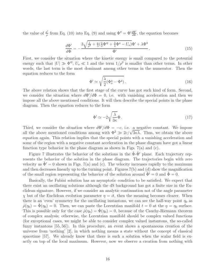
Figure 7 illustrates the behavior of the solutions in the Φ-Φ′ plane. Each trajectory rep-resents the behavior of the solution in the phase diagram. The trajectories begin with zerovelocity as Φ′ = 0 shown in Figs. 7(a) and (c). The velocity increases rapidly to the maximumand then decreases linearly up to the turning point. Figures 7(b) and (d) show the magnificationof the small region representing the behavior of the solution around Φ′ = 0 and Φ = 0.

Basically, the Fubini solution has an asymptotic condition to be satisfied. We expect thatthere exist an oscillating solutions although the dS background has got a finite size in the Eu-clidean signature. However, if we consider an analytic continuation not of the angle parameterχ but of the Euclidean evolution parameter η = it, then the meaning becomes clearer. Whenthere is an ‘even’ symmetry for the oscillating instantons, we can see the half-way point η0 asρ(η0) = Φ(η0) = 0. Then, we can paste the Lorentzian manifold t = 0 at the η = η0 surface.This is possible only for the case ρ(η0) = Φ(η0) = 0, because of the Cauchy-Riemann theoremof complex analysis; otherwise, the Lorentzian manifold should be complex valued functions(for exceptional cases, we might be able to consider complex valued instantons, the so-calledfuzzy instantons [55, 56]). In this procedure, an event shows a spontaneous creation of theuniverse from ‘nothing’ [2], in which nothing means a state without the concept of classicalspacetime [57]. We already know that there is such a solution when the scalar field is ex-actly on top of the local maximum. However, now we observe a creation from nothing with

16

-0.25 0.00 0.25

-0.03

0.03 Φ0= -1 Φ0= -2 Φ0= -3 Φ0= -4 Φ0= -5 Φ0= -6 Φ0= -7

'

(d)

-8 -4 0

0

4

Φ0= -1 Φ0= -2 Φ0= -3 Φ0= -4 Φ0= -5 Φ0= -6 Φ0= -7

'

(c)

-0.25 0.00 0.25

-0.03

0.03 Φ0= -1 Φ0= -2 Φ0= -3 Φ0= -4 Φ0= -5 Φ0= -6 Φ0= -7

'

(b)

-8 -4 0

0

4

Φ0= -1 Φ0= -2 Φ0= -3 Φ0= -4 Φ0= -5 Φ0= -6 Φ0= -7

'

(a)

B. the initial AdS background

A. the initial flat background

Figure 7: The behavior of the solutions represented in the phase diagram.

17

highly non-trivial field dynamics. This is worthwhile to be highlighted and we postpone furtheranalysis for the future work.

3.3 Fubini instantons with Z2 symmetry

We now shift our attention to the new type of solutions in the initial background as the dSspace, i.e. Uo > 0. The Euclidean dS space has a compact geometry. Thus the solutions canhave Z2 symmetry. We consider the boundary conditions in Eq. (12). To obtain the solutionswith Z2 symmetry, we need to impose additional conditions. For the background geometry,ρ′ = 0 at η = ηmax

2. On the other hand, for the scalar field, we impose Φ = 0 at η = ηmax

2for

the solutions with odd number of crossings of the potential well and Φ′ = 0 at η = ηmax

2for

the solutions with even number of crossings. The solutions with odd number of crossing havethe opposite state of the value Φ at η = 0 and η = ηmax, i.e. Φ|η=ηmax

= −Φo. The solutionswith even number of crossing have the same state of the value Φ at η = 0 and η = ηmax, i.e.Φ|η=ηmax

= Φo. We stress that the boundary conditions in Eq. (12) gives rise to completely newtype of solutions of Fubini instanton.

Figure 8 shows the numerical solutions of the Fubini instanton with Z2 symmetry. We takeκ = 0.50 and Uo = 0.03. Thus the dS region in the Φ-space spans the region −0.589 . Φ .0.589. We consider four cases with different initial positions of Φ. Figure 8(a) illustrates thenumerical solution of Φ. The trajectories with the blue and red color go back to the sameposition of Φ in the presence of the inverted potential, i.e. they have even number of crossings.The trajectories with the black and green color go back to the opposite position of Φ, i.e. theyhave odd number of crossings. Figure 8(b) depicts the numerical solution of ρ. Figures 8(c) and(d) illustrate the behavior of the solutions in the Φ-Φ′ plane. Each trajectory represents thebehavior of the solution in the phase diagrams. The blue and red lines indicate that the interiorpart of two instantons has got the same state as Φ, whereas the green and black lines indicatethat the interior part has got the opposite state of Φ. Figure 8(d) illustrates the magnificationof a small region representing the behavior of the solution around Φ′ = 0 and Φ = 0. Figure8(e) illustrates the volume energy density, where the density has got a form ξ = −U . The boxshows the magnification of a small region representing behavior of curves. The densities in eachof the case have got positive values near the initial starting point Φo far away from the pointΦ = 0, because the densities have the form ξ = −U and Uo > 0. The solutions oscillate in thedS region as found the present work. The density always negative values for the case of theblack line. Figure 8(f) illustrates the Euclidean energy Eξ = 2π2ρ3ξ for each slice of constant ηvalues. The negative energy parts in each of the case signifies a rolling state in the dS region.Table 4 shows the initial value of Φ, colors of the plot used, and the actions obtained from Fig.8.

18

-0.5 0.0 0.5

-0.2

0.0

0.2

' =-0.3787513662 =-2.45703 =-3.9490198 =-5.145680234

(d)

-5 0 5

-5

0

5

' =-0.3787513662 =-2.45703 =-3.9490198 =-5.145680234

(c)

0 20 400

8

16

=-0.3787513662 =-2.45703 =-3.9490198 =-5.145680234

(b)

0 20 40

-5

0

5

=-0.3787513662 =-2.45703 =-3.9490198 =-5.145680234

(a)

0 20 40

0

150

0 10 20 30 40-0.030

-0.025

-0.020

=-0.3787513662 =-2.45703 =-3.9490198 =-5.145680234

(e)

0 10 20 30 40

-1200

-600

0

=-0.3787513662 =-2.45703 =-3.9490198 =-5.145680234

(f)

Figure 8: (color online). The numerical solutions of the Fubini instanton with Z2 symmetry.

19

Φ0 Color of plot Scs Sbg B

−0.37875 Black −3.15525× 104 −3.15827× 104 30.2

−2.45703 Red −3.15176× 104 −3.15827× 104 65.2

−3.94902 Green −3.14005× 104 −3.15827× 104 182.2

−5.14568 Blue −3.10727× 104 −3.15827× 104 510.0

Table 4: The dimensionless variables and the color of plot used, and the actions obtained in Fig. 8.

4 Causal structures

In this section, we briefly outline the causal structure of the solutions in the Lorentzian signa-ture. Due to the pressure difference, the nucleated AdS region will expand over the backgroundand hence the boundary of the nucleated AdS region will be time-like.

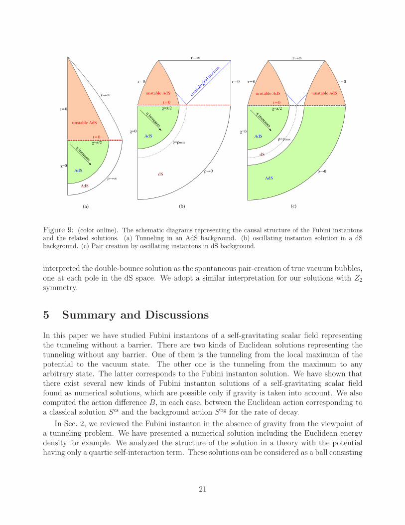
Figure 9 shows the schematic diagrams representing the causal structures of the Fubiniinstantons and the related solutions. The χ = π/2 surface can be analytically continued to thesurface t = 0 in the Lorentzian signature. The lower vacuum region in the instanton (greencolored region) will be unstable during the Lorentzian time evolution (orange colored region).Due to the instability of the Fubini type potential, the whole causal structure may depend onthe shape of the potential or the vacuum structure i.e. whether the left or the right side of thepotential has true vacua or not. Therefore, the followings are meaningful only as reasonableestimations for general behavior and these may be different for special examples.

Figure 9(a) illustrates the instanton solution in an AdS background. It will form time-liker = 0 and r = ∞ boundaries in the Lorentzian signature. However, the AdS region may beunstable to form a kind of singularity. Figure 9(b) illustrates the instanton solution in thedS background. The dS region has a cosmological horizon and will this form a future infinity.The AdS region (orange colored region) will expand over the dS region due to the pressuredifference. Figure 9(c) is the pair creation by the oscillating instanton solutions. Therefore,in the instanton part, the dS region around the ρ = ρmax is surrounded by the AdS (greencolored region) part. In the Lorentzian signature, we can interpret these two AdS parts asbeing nucleated in a dS background. In Fig. 9(c), we infer that, there still remains a dS regionand a future infinity.

The pair creation of the instantons in this work is quite different from the ordinary quantumprocess of pair creation of particles. We take the initial background as the dS space, i.e. Uo > 0.The Euclidean dS space has a compact geometry. Thus, the geometry has two poles. If oneobject is created on the north pole and the other on the south pole, we can interpret thatprocess as the pair creation of objects. As an example of the process, the two-crossing solutionbetween the sides of the potential barrier in the double-well potential was considered as atype of a double-bounce solution or an anti-double-bounce solution [58], in which the authors

20

dS

AdS

η increases

χ=π/2

χ=0

ρ→0

t=0

r=0

r→∞

unstable AdS

ρ=ρmax

r=0

cosm

olog

ical

hor

izon

AdS

AdS

η increases

χ=π/2

χ=0

ρ→∞

t=0

r=0

r→∞

unstable AdS

dS

AdS

η increases

χ=π/2

χ=0

ρ→0

t=0

r=0

r→∞

unstable AdS

ρ=ρmax

r=0

unstable AdS

AdS

(a) (b) (c)

Figure 9: (color online). The schematic diagrams representing the causal structure of the Fubini instantonsand the related solutions. (a) Tunneling in an AdS background. (b) oscillating instanton solution in a dSbackground. (c) Pair creation by oscillating instantons in dS background.

interpreted the double-bounce solution as the spontaneous pair-creation of true vacuum bubbles,one at each pole in the dS space. We adopt a similar interpretation for our solutions with Z2

symmetry.

5 Summary and Discussions

In this paper we have studied Fubini instantons of a self-gravitating scalar field representingthe tunneling without a barrier. There are two kinds of Euclidean solutions representing thetunneling without any barrier. One of them is the tunneling from the local maximum of thepotential to the vacuum state. The other one is the tunneling from the maximum to anyarbitrary state. The latter corresponds to the Fubini instanton solution. We have shown thatthere exist several new kinds of Fubini instanton solutions of a self-gravitating scalar fieldfound as numerical solutions, which are possible only if gravity is taken into account. We alsocomputed the action difference B, in each case, between the Euclidean action corresponding toa classical solution Scs and the background action Sbg for the rate of decay.

In Sec. 2, we reviewed the Fubini instanton in the absence of gravity from the viewpoint ofa tunneling problem. We have presented a numerical solution including the Euclidean energydensity for example. We analyzed the structure of the solution in a theory with the potentialhaving only a quartic self-interaction term. These solutions can be considered as a ball consisting

21

of only a thick wall except for the one point at the center of the solution with a lower arbitrarystate than the outer vacuum state unlike a vacuum bubble which consists of an inner part witha lower vacuum state and a wall.

In Sec. 3, we have studied the instanton solutions in curved space. We performed carefulnumerical study to solve the coupled equations for the gravity and the scalar field simultane-ously. We have shown that there exist numerical solutions without any oscillation in the initialAdS space for the potential with only the quartic term. We have also shown that there existnumerical solutions for the potential with both a quartic and a quadratic term irrespectiveof the value of the cosmological constant. For this particular case, there is no solution withan O(4) symmetry when gravity is switched off. In order to estimate the decay rate of thebackground state, we calculated the action difference between the action of the solution andthat of the background obtained using numerical means.

We have obtained oscillating Fubini instantons as new types of solutions. We have shownthat there exist oscillating numerical solutions for the potential with only the quartic term inthe flat and AdS space, except for the solution without oscillation in the initial AdS space withthe specific value of a cosmological constant and the parameters. We have analyzed the behaviorof the solutions using the phase diagram method. The oscillation dies away asymptotically inboth the flat and the AdS space.

We have obtained numerical solutions representing the Fubini instanton with Z2 symmetry.We stress that they represent completely new type of solutions of Fubini instanton. Thesesolutions can be interpreted as the pair creation with each one having the same state and witheach one having the opposite state, respectively. The solutions can lead to more interestinginterpretation as follows: any arbitrary state can tunnel into another arbitrary state with anO(4)-symmetry in the curved spacetime, although no vacuum state exists as the instantonsolution. The solutions are possible as long as the maximum of the potential remains positive.

The subject on the pair creation of bubbles was first considered in Ref. [59]. The numericalsolution representing the pair of solutions is in Fig. 2 in Ref. [58], which can be interpreted asthe pair creation of the bubbles, one at each pole in the dS space. However, there is a differentinterpretation on the solutions [53, 60], in which the authors studied a decay channel of deSitter vacua. The solutions with O(3) symmetry can be understood as describing tunnelingin a finite horizon volume at finite temperature. The solutions maybe correspond to thermalproduction of a bubble in their interpretation. In this stage, the comparative analysis betweenthe O(4)-symmetric solution and O(3)-symmetric solution with respect to the pair creation isneeded to be studied more. We leave this for future work.

In Sec. 4, we have analyzed the schematic diagrams representing the causal structures of theFubini instantons and the related solutions in the Lorentzian signature. For the special caserepresenting the solution with Z2 symmetry, the dS region around the ρ = ρmax is surroundedby an AdS part.

We now mention on the negative mode problem. It was known that the bounce solutionhas one negative mode in the spectrum of small perturbations about the solution [46,61]. The

22

bounce solution with one negative mode corresponds to the tunneling process in the lowestWKB approximation. In Ref. [61], Coleman argued that the Euclidean solution with only onenegative mode is related to the tunneling process in the flat Minkowski spacetime. However,there is no rigorous proof on extension of Coleman’s argument to the curved space claimingthe physical irrelevance of the solutions with additional negative modes. For example, thetime-translation invariance, or zero modes, is one of crucial elements to prove the uniquenessof the negative mode in his argument. However, the existence of zero modes is not guaranteedin curved spacetime. Another point is that the Euclidean time interval is at most of O(H−1) inde Sitter space. Hence, only a finite number of the bounces can be placed far apart from eachother. Therefore, the dilute gas approximation may become invalid easily, which leads to thebreakdown of the WKB approximation [62]. There appears diverse situations on the negativemodes when the gravity is taken into account [62–65]. Although, the bounce solution with onenegative mode in curved space dominates the tunneling process, the solutions with additionalnegative modes may also contribute to the tunneling process. There exist some works includingthe physical interpretation on the oscillating solutions with more than one negative mode. Onecan naturally interpret the system in de Sitter background as a thermal system. The authors inRefs. [51,53] interpreted that the existence of additional negative modes represents the solutionsas unstable intermediate thermal configuration. They seem to observe the clue to support thisidea on the other point of view. It is known that the N times oscillating solutions have Nnegative modes [51,53,66]. The even numbers of negative modes of the form 4N and 4N +2 donot have imaginary part of the energy, while the odd numbers of negative modes of the form4N + 3 have the imaginary part of the energy with the wrong sign. However, 4N + 1 negativemodes may have a meaning for a tunneling process even if the solution may not be related tothe lowest WKB approximation. Recently the analysis on the negative modes of oscillatinginstantons has been investigated [66]. The oscillating instantons as homogeneous tunnelingchannels have been also studied [67]. In conclusion, we believe many Euclidean solutions incurved space with zero and negative modes may have physical significance and deserves furtherinvestigation.

In summary, we illustrate the following finding in our new contribution regarding this issue:

1. In the absence of gravity, a −φ4-type potential has infinitely many instanton solutionswhereas a −φ4 + φ2-type potential has no instanton solution. However, the inclusion of

the gravity changes all the situation abruptly : for the former case, the solution space getreduced to a finite space and for the latter case, there exists solutions.

2. We also confirm that −φ4-type potentials have oscillating instanton solutions as well asthe solutions with Z2 symmetry.

Therefore, the Fubini instanton is one of the few examples that shows the effect of gravitybringing drastic changes to the tunneling process. There can be more applications of theoscillating instantons and we confirm that the Fubini-type potentials also contribute largelytowards these processes. We postpone any possible application of such oscillating solutionsincluding the phase space of solutions for our future work [48].

23

6 Acknowledgements

We would like to thank Andrei Linde for kind historic comments on the inflationary multiversescenario and Fubini instanton. We would like to thank Erick J. Weinberg, George Lavrelashvili,Hongsu Kim, Yunseok Seo, and Dong-il Hwang for helpful discussions and comments, and thankChaitali Roychowdhury for a careful English revision of the manuscript. We would like to thankManu B. Paranjape and Richard MacKenzie for their hospitality during our visit to Univer-site de Montreal. This work was supported by the Korea Science and Engineering Foundation(KOSEF) grant funded by the Korea government(MEST) through the Center for QuantumSpacetime(CQUeST) of Sogang University with grant number R11 - 2005 - 021. WL was up-ported by Basic Science Research Program through the National Research Foundation of Ko-rea(NRF) funded by the Ministry of Education, Science and Technology(2012R1A1A2043908).DY is supported by the JSPS Grant-in-Aid for Scientific Research (A) No. 21244033. Weappreciate APCTP for its hospitality during completion of this work.

24

References

[1] A. D. Linde, Nonsingular regenerating inflationary universe, Cambridge Universitypreprint, Print-82-0554.

[2] A. Vilenkin, Phys. Rev. D 27, 2848 (1983); arXiv: gr-qc/0409055.

[3] A. D. Linde, Phys. Lett. B 175, 395 (1986).

[4] A. H. Guth, Phys. Rep. 333-334, 555 (2000).

[5] S. Winitzki, Lect. Notes Phys. 738, 157 (2008).

[6] R. Bousso and J. Polchinski, J. High Energy Phys. 06 (2000) 006.

[7] L. Susskind, arXiv: hep-th/0302219.

[8] J. Garriga and A. Vilenkin, Phys. Rev. D 57, 2230 (1998).

[9] A. Borde, A. H. Guth, and A. Vilenkin, Phys. Rev. Lett. 90, 151301 (2003).

[10] A. Mithani and A. Vilenkin, arXiv:1204.4658; L. Susskind, arXiv:1204.5385;arXiv:1205.0589.

[11] S. Kachru, R. Kallosh, A. Linde, and S. P. Trivedi, Phys. Rev. D 68, 046005 (2003).

[12] S. K. Ashok and M. R. Douglas, J. High Energy Phys. 01 (2004) 060.

[13] C. M. Hull, Classical Quantum Gravity 2, 343 (1985).

[14] R. Kallosh, A. Linde, S. Prokushkin, and M. Shmakova, Phys. Rev. D 65, 105016 (2002);ibid. D 66, 123503 (2002).

[15] R. Kallosh and A. Linde, Phys. Rev. D 67, 023510 (2003).

[16] H. Kim, J. High Energy Phys. 01 (2003) 080.

[17] A. A. Belavin, A. M. Polyakov, A. S. Schwartz, and Yu. S. Tyupkin, Phys. Lett. 59B, 85(1975).

[18] S. Coleman, Aspects of symmetry (Cambridge University Press, Cambridge, England,1985).

[19] I. Herbut, A Modern Approach to Critical Phenomena (Cambridge University Press, Cam-bridge, 2007).

[20] M. B. Voloshin, I. Yu. Kobzarev, and L. B. Okun, Yad. Fiz. 20, 1229 (1974) [Sov. J. Nucl.Phys. 20, 644 (1975)].

25

[21] S. Coleman, Phys. Rev. D 15, 2929 (1977); ibid. D 16, 1248(E) (1977).

[22] S. Coleman and F. De Luccia, Phys. Rev. D 21, 3305 (1980).

[23] S. Parke, Phys. Lett. 121B, 313 (1983).

[24] K. Lee and E. J. Weinberg, Phys. Rev. D 36, 1088 (1987).

[25] B.-H. Lee and W. Lee, Classical Quantum Gravity 26, 225002 (2009).

[26] S. Fubini, Nuovo Cimento A 34, 521 (1976).

[27] A. D. Linde, Nucl. Phys. B216, 421 (1983); ibid. B223, 544(E) (1983).

[28] K. Lee and E. J. Weinberg, Nucl. Phys. B267, 181 (1986); K. Lee, Nucl. Phys. B282, 509(1987).

[29] L. G. Jensen and P. H. Steinhardt, Nucl. Phys. B317, 693 (1989).

[30] B.-H. Lee, C. H. Lee, W. Lee, and C. Oh, Phys. Rev. D 85, 024022 (2012).

[31] S. Kanno, M. Sasaki, and J. Soda, Classical Quantum Gravity 29, 075010 (2012); Prog.Theor. Phys. 128, 213 (2012).

[32] J. Garriga, X. Montes, M. Sasaki, and T. Tanaka, Nucl. Phys. B 551, 317 (1999).

[33] S. Khlebnikov, Nucl. Phys. B 631, 307 (2002).

[34] F. Loran, Mod. Phys. Lett. A 22, 2217 (2007).

[35] S. de Haro and A. C. Petkou, J. High Energy Phys. 12 (2006) 076; S. de Haro, I. Papadim-itriou, and A. C. Petkou, Phys. Rev. Lett. 98, 231601 (2007).

[36] J. L. F. Barbon and E. Rabinivici, J. High Energy Phys. 04 (2010) 123; J. High EnergyPhys. 04 (2011) 044.

[37] A. N. Kuznetsov and P. G. Tinyakov, Mod. Phys. Lett. A 11, 479 (1996); Phys. Rev. D56, 1156 (1997).

[38] A. A. Yurova and A. V. Yurov, Phys. Lett. A 372, 4222 (2008).

[39] C. M. Bender and T. T. Wu, Phys. Rev. D 7, 1620 (1973); J.-Q. Liang and H. J. W. Muller-Kirsten, Phys. Rev. D 45, 2963 (1992); ibid. D 48, 964(E) (1993).

[40] L. N. Lipatov, Sov. Phys. JETP 45, 216 (1977).

[41] I. Affleck, Nucl. Phys. B191, 429 (1981).

26

[42] J. W. York, Jr., Phys. Rev. Lett, 28, 1082 (1972); G. W. Gibbons and S. W. Hawking,Phys. Rev. D 15, 2752 (1977); J. W. York, Jr., Found. Phys. 16, 249 (1986).

[43] C. W. Misner, K. S. Thorne, and J. A. Wheeler, Gravitation (Freeman, San Francisco,1973).

[44] B. K. Berger, Gen. Rel. Grav. 38, 625 (2006).

[45] W. H. Press, S. A. Teukolsky, W. T. Vetterling, and B. P. Flannery, Numerical Recipes in

Fortran (Cambridge University Press, Cambridge, England, 1992).

[46] C. G. Callan, Jr. and S. Coleman, Phys. Rev. D 16, 1762 (1977).

[47] E. J. Weinberg, Phys. Rev. D 47, 4614 (1993); J. Baacke and G. Lavrelashvili, Phys. Rev.D 69, 025009 (2004); G. V. Dunne and H. Min, Phys. Rev. D 72, 125004 (2005).

[48] B.-H. Lee, W. Lee, D. Ro, and D.-h. Yeom, in progress.

[49] G. W. Gibbons, S. W. Hawking, and M. J. Perry, Nucl. Phys. B138, 141 (1978).

[50] A. Dasgupta and R. Loll, Nucl. Phys. B 606, 357 (2001).

[51] J. C. Hackworth and E. J. Weinberg, Phys. Rev. D 71, 044014 (2005); E. J. Weinberg,AIP Conf. Proc. 805, 259 (2005).

[52] G .V. Lavrelashvili, Phys. Rev. D 73, 083513 (2006); G. V. Dunne and Q.-h. Wang, Phys.Rev. D 74, 024018 (2006).

[53] A. R. Brown and E. J. Weinberg, Phys. Rev. D 76, 064003 (2007).

[54] A. Vilenkin, Phys. Rev. Lett. 72, 3137 (1994); A. Linde, Phys. Lett. B 327, 208 (1994).

[55] J. B. Hartle, S. W. Hawking, and T. Hertog, Phys. Rev. Lett. 100, 201301 (2008); Phys.Rev. D 77, 123537 (2008).

[56] D.-i. Hwang, H. Sahlmann, and D.-h. Yeom, Classical Quantum Gravity 29, 095005 (2012);D.-i. Hwang, B.-H. Lee, H. Sahlmann, and D.-h. Yeom, Classical Quantum Gravity 29,175001 (2012).

[57] A. Vilenkin, Nucl. Phys. B252, 141 (1985).

[58] R. Bousso and A. Linde, Phys. Rev. D 58, 083503 (1998).

[59] J. Garriga and A. Megevand, Phys. Rev. D 69, 083510 (2004); Int. J. Theor. Phys. 43,883 (2004).

[60] A. Masoumi and E. J. Weinberg, Phys. Rev. D 86, 104029 (2012).

27

[61] S. R. Coleman, Nucl. Phys. B298, 178 (1988).

[62] T. Tanaka and M. Sasaki, Prog. Theor. Phys. 88, 503 (1992); T. Tanaka, Nucl. Phys.B556, 373 (1999).

[63] A. R. Brown and A. Dahlen, Phys. Rev. D 84, 105004 (2011).

[64] G. V. Lavrelashvili, V. A. Rubakov, and P. G. Tinyakov, Phys. Lett. 161B, 280 (1985).

[65] A. Khvedelidze, G. Lavrelashvili, and T. Tanaka, Phys. Rev. D 62, 083501 (2000);G. Lavrelashvili, Nucl. Phys. B, Proc. Suppl. 88, 75 (2000).

[66] L. Battarra, G. Lavrelashvili and J.-L. Lehners, Phys. Rev. D 86, 124001 (2012).

[67] B.-H. Lee, W. Lee, and D.-h. Yeom, arXiv:1206.7040 [hep-th].

28