Embed Size (px)
Citation preview

CONTRIBUTED RESEARCH ARTICLES 163
fslr: Connecting the FSL Software with Rby John Muschelli, Elizabeth Sweeney, Martin Lindquist, and Ciprian Crainiceanu
Abstract We present the package fslr, a set of R functions that interface with FSL (FMRIB SoftwareLibrary), a commonly-used open-source software package for processing and analyzing neuroimagingdata. The fslr package performs operations on ‘nifti’ image objects in R using command-linefunctions from FSL, and returns R objects back to the user. fslr allows users to develop imageprocessing and analysis pipelines based on FSL functionality while interfacing with the functionalityprovided by R. We present an example of the analysis of structural magnetic resonance images,which demonstrates how R users can leverage the functionality of FSL without switching to shellcommands.
Glossary of acronymsMRI Magnetic Resonance Imaging/Image FSL FMRIB Software LibraryPD Proton Density FAST FMRIB’s Automated Segmentation Tool
FLAIR Fluid-Attenuated Inversion Recovery FLIRT FMRIB’s Linear Image Registration ToolMS Multiple Sclerosis BET Brain Extraction Tool
FMRIB Functional MRI of the Brain Group FNIRT FMRIB’s Nonlinear Image Registration ToolMNI Montreal Neurological Institute
Introduction
FSL (FMRIB Software Library) is a commonly-used software for processing and analyzing neuroimag-ing data (Jenkinson et al., 2012). This software provides open-source, command-line tools and agraphical user interface (GUI) for image processing tasks such as image smoothing, brain extraction(Smith, 2002), bias-field correction, segmentation (Zhang et al., 2001), and registration (Jenkinson andSmith, 2001; Jenkinson et al., 2002). Many of these functions are used extensively in medical imagingpipelines. According to a recent survey paper by Carp (2012), 13.9% of published neuroimagingstudies used FSL.
There exist a number of R packages for reading and manipulating image data, including Ana-lyzeFMRI (Bordier et al., 2011), RNiftyReg (Clayden, 2015), and fmri (Tabelow and Polzehl, 2011)(see the Medical Imaging CRAN task view http://CRAN.R-project.org/view=MedicalImaging formore information). Although these packages are useful for performing image analysis, much of thefundamental functionality that FSL and other imaging software provide is not currently implementedin R. In particular, this includes algorithms for performing slice-time correction, motion correction,brain extraction, tissue-class segmentation, bias-field correction, co-registration, and normalization.This lack of functionality is currently hindering R users from performing complete analysis of imagedata within R. Instead of re-implementing FSL functions in R, we propose a user-friendly interfacebetween R and FSL that preserves all the functionality of FSL, while retaining the advantages of usingR. This will allow R users to implement complete imaging pipelines without necessarily learningsoftware-specific syntax.
The fslr package relies heavily on the oro.nifti (Whitcher et al., 2011) package implementation ofimages (referred to as ‘nifti’ objects) that are in the Neuroimaging Informatics Technology Initiative(NIfTI) format, as well as other common image formats such as ANALYZE. oro.nifti also providesuseful functions for plotting and manipulating images. fslr expands on the oro.nifti package byproviding additional functions for manipulation of ‘nifti’ objects.
fslr workflow
The general workflow for most fslr functions that interface with FSL is as follows:
1. Filename or ‘nifti’ object is passed to fslr function.
2. FSL command is created within fslr function and executed using the system command.
3. Output is written to disk and/or read into R and returned from the function.
From the user’s perspective, the input/output process is all within R. The advantage of thisapproach is that the user can read in an image, do manipulations of the ‘nifti’ object using standardsyntax for arrays, and pass this object into the fslr function without using FSL-specific syntax writtenin a shell language. Also, one can perform image operations using FSL, perform operations on the‘nifti’ object in R that would be more difficult using FSL, and then perform additional operationsusing FSL by passing that object to another fslr command. Thus, users can create complete pipelinesfor the analysis of imaging data by accessing FSL through fslr.
The R Journal Vol. 7/1, June 2015 ISSN 2073-4859
CONTRIBUTED RESEARCH ARTICLES 164
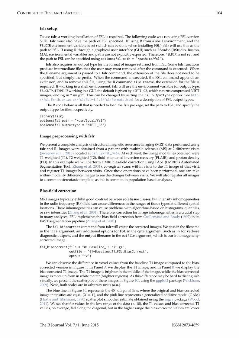
fslr setup
To use fslr, a working installation of FSL is required. The following code was run using FSL version5.0.0. fslr must also have the path of FSL specified. If using R from a shell environment, and theFSLDIR environment variable is set (which can be done when installing FSL), fslr will use this as thepath to FSL. If using R through a graphical user interface (GUI) such as RStudio (RStudio, Boston,MA), environmental variables and paths are not explicitly exported. Therefore, FSLDIR is not set, andthe path to FSL can be specified using options(fsl.path = "/path/to/fsl").
fslr also requires an output type for the format of images returned from FSL. Some fslr functionsproduce intermediate files that the user may want removed after the command is executed. Whenthe filename argument is passed to a fslr command, the extension of the file does not need to bespecified, but simply the prefix. When the command is executed, the FSL command appends anextension, and to remove this file, using the R command file.remove, the extension for the file isrequired. If working in a shell environment, fslr will use the environment variable for output type:FSLOUTPUTTYPE. If working in a GUI, the default is given by NIFTI_GZ, which returns compressed NIfTIimages, ending in “.nii.gz”. This can be changed by setting the fsl.outputtype option. See http://fsl.fmrib.ox.ac.uk/fsl/fsl-4.1.9/fsl/formats.html for a description of FSL output types.
The R code below is all that is needed to load the fslr package, set the path to FSL, and specify theoutput type for files, respectively.
library(fslr)options(fsl.path = "/usr/local/fsl")options(fsl.outputtype = "NIFTI_GZ")
Image preprocessing with fslr
We present a complete analysis of structural magnetic resonance imaging (MRI) data performed usingfslr and R. Images were obtained from a patient with multiple sclerosis (MS) at 2 different visits(Sweeney et al., 2013), located at bit.ly/FSL_Data. At each visit, the image modalities obtained wereT1-weighted (T1), T2-weighted (T2), fluid-attenuated inversion recovery (FLAIR), and proton density(PD). In this example we will perform a MRI bias-field correction using FAST (FMRIB’s AutomatedSegmentation Tool; Zhang et al. 2001), co-register scans within visits to the T1 image of that visit,and register T1 images between visits. Once these operations have been performed, one can takewithin-modality difference images to see the changes between visits. We will also register all imagesto a common stereotaxic template, as this is common in population-based analyses.
Bias-field correction
MRI images typically exhibit good contrast between soft tissue classes, but intensity inhomogeneitiesin the radio frequency (RF) field can cause differences in the ranges of tissue types at different spatiallocations. These inhomogeneities can cause problems with algorithms based on histograms, quantiles,or raw intensities (Zhang et al., 2001). Therefore, correction for image inhomogeneities is a crucial stepin many analyses. FSL implements the bias-field correction from Guillemaud and Brady (1997) in itsFAST segmentation pipeline (Zhang et al., 2001).
The fsl_biascorrect command from fslr will create the corrected images. We pass in the filenamein the file argument, any additional options for FSL in the opts argument, such as -v for verbosediagnostic outputs, and the output filename in the outfile argument, which is our inhomogeneity-corrected image.
fsl_biascorrect(file = "01-Baseline_T1.nii.gz",outfile = "01-Baseline_T1_FSL_BiasCorrect",opts = "-v")
We can observe the difference in voxel values from the baseline T1 image compared to the bias-corrected version in Figure 1. In Panel A we display the T1 image, and in Panel B we display thebias-corrected T1 image. The T1 image is brighter in the middle of the image, while the bias-correctedimage is more uniform in white matter (brighter regions). As this difference may be hard to distinguishvisually, we present the scatterplot of these images in Figure 1C, using the ggplot2 package (Wickham,2009). Note, both scales are in arbitrary units (a.u.).
The blue line in Figure 1C represents the 45◦ diagonal line, where the original and bias-correctedimage intensities are equal (X = Y), and the pink line represents a generalized additive model (GAM)(Hastie and Tibshirani, 1990) scatterplot smoother estimate obtained using the mgcv package (Wood,2011). We see that for values in the low range of the data (< 10), the T1 values and bias-corrected T1values, on average, fall along the diagonal, but in the higher range the bias-corrected values are lower.
The R Journal Vol. 7/1, June 2015 ISSN 2073-4859

CONTRIBUTED RESEARCH ARTICLES 165
C0
50
100
150
200
0 100 200T1 Values (a.u.)
Bia
s−F
ield
−C
orre
cted
T1
Val
ues
(a.u
.)
X = Y LineGAM
Comparison of T1 Values and Bias−Corrected Values
●
●
●
●
●
●●
●●●
●
●
●●
●●
●
●
●
●
●
●
●
●
●
●
●
●
●
●
●
●
●●
●
●
●
●
●
●
●
●
●
●
●
●
●●
●
●●●
●
●●
●
●
●
●
●
●
●
●
●
●
●
●●
●
●
●
●
●
●●
●●
●
●
●
●
●
●
●
●
●
●
●
●
●
●●
●●●
●
●
●
●
●
●
●
●
●
●
● ●
●
●
●●
●
●
●
●●
●
●
●
●
●
●
●
●
●
●
●●
●
●
●
●
●●
●
●
●
●
●
●
●
●
●
●
●
●●●
●
●
●
●●
●
●
●
●
●
●
●
●
●
●
●
●
●●
●
●
●
●
●
●●
●
●
●
●
●●
●
●
●
●
●
●
●●
●●
●
●
●
●
●
●
●
●●
●
●
●
●●●●
●
●
●
●
●
●
●
●
●●●
●
●
●
●
●
●
●●
●
●
●
●●
●
●
●
●
●
●
●●
●
●
●
●
●
●●
●
●
●
●
●
●●
●
●
●●
●
●●
●
●
●
●
●●
●●
●
●
●
●
●
●
●
●
●●
●●
●
●
●
●
●●
●
●
●
●
●
●
●
●●
●
●
●
●
●
●
●
●
●
●
●
●●●●
●
●
●
●
●
●
●
●
●
●
●
●
●
●●
●
●
●
●
●
●
●
●
●
●
●
●
●
●
●
●
●
●
●
●
●
●
●
●
●
●●
● ●
●
●●
●
●●
●●
●
●
●●●
●
●
●
●
●●
●
●
●
●
●
●
●
●
●
●
●
●
●
●●
●●
●
●●
●
●
●
●
●
●
●
●
●
●
●
●
●●
●
●
●●
●
●
●
●
●
●
●
●
●
●
●
●
●
●
●
●
●
●
●
●
●
●
●
●
●
●
●
●
●
●●
●
●
●
●
●
●
●
●
●
●
●
●
●
●
●
●
●
●●
●●
●
●
●
●
●
●
●
●
●
●
●
●
●●
●
●
●
●
●
●
●
●
●●
●
●
●
●
●
●
●
●
●●
●
●●
●
●
●
●
●
●●
●
●
●
●
●
●
●
●
●
●
●
●
●
●
●
●
●
●
●
●
●
●●
●
●
●
●
●
●
●
●
●
●●
●
●
●
●
●
●●
●
●●
●
●
●
●
●●
●
●
●
●
●
●
●
●
●
●
●
●
●
●
●
●
●
●
●
●
●
●●
●
●
●
●
●
●
●
●
●
●
●
●
●
●
●
●
●
●
●●
●
●
●
●
●
●
●
●
●
●
●●
●
●
●
●
●
●
●
●
●
●
●
●
●
●
●●
●
●
●
●
●
●
●
●
●
●
●
●
●
●
●
●
●●
●●
●
●
●
●
●
●
●
●●
●
●
●
●●
●
●●
●
●
●
●
●
●
●
●
●●
●
●
●
●
●
●
●
●
●
●
●
●
●
●
●
●
●
●
●
●
●●
●
●
●
●
●
●
●
●
●
●
●
●
●
●
●
●
●
●
●●
●
●
●
●
●
●
●
●
●
●
●
●
●
●
●
●
●
●
●
●
●
●
●
●
●
●
●
●●
●
●
●
●
●●●
●●●
●●
●
●
●
●
●
●
●
●
●
●
●
●
●
●
●
●
●
●
●
●●●
●
●
●
●
●
●●
●
●
●
●
●
●
●
●
●●
●
●
●
●
●●
●
●
●
●
●
●
●
●
●
●
●
●
●
●
●
●
●
●
●
●
●
●●
●
●
●
●
●
●
●
●
●
●
●
●
●
●
●
●
●
●●
●
●
●
●
●
●
●
●
●
●
●
●
●●
●
●
●
●
●
●
●
●●
●
●
●
●
●
●
●
●
●
●
●
●
●
●
●
●
●
●●
●
●
●
●
●●
●
●
●
●
●
●
●
●
●
●
●
●
●
●
●
●
●
●
●
●
●●
●●
●
●
●
●
●
●
●
●
●
●
●●
●●
●
●●
●
●●
●●
●
●
●
●
●
●
●●
●
●
●
●●
●●●●●
●
●
●
●
●
●●
●
●
●
●
●
●●
●
●
●
●●
●
●
●
●
●
●
●●
●●
●
●
●
●
●
●●●
●
●
●
●
●
●
●
●
●
●
●
●●
●
●
●
●
●
● ●●
●
●
●
●
●
●
●●
●
●
●
●
●
●
●
●●
●
●
●
●
●
●
●
●
●
●
●●
●
●
●
●
●
●
●
●
●
●
●
●
●
●
●
●
●
●●
●
●
●
●
●
●
●●
●●
●
●
●
●
●
●
●
●
●
●
●●
●
●●
●
●
●
●
●
●
●
●
●
●
●
●
●●●●
●●
●
●
●●
●●
●
●
●
●
●
●
●
●
●
●
●
●
●
●
●
●
●
●
●
●
●
●
●●
●●
●
●
●
●
●
●●
●
●●●
●
●
●
●
●
●
●
●
●●
●
●
●
●
●
●●
●
●
●
●
●
●
●
●
●●●
●
●
●●●●●
●
●
●
●
●
●
●
●
●
●
●
●●●
●
●
●
●
●
●●
●
●●
●●
●
●●
●
●
●●
●
●
●
●
●
●
●●
●
●
●
●
●
●
●
●
●
●
●
●
●
●
●
●
●
●
●
●
●
●
●
●
●
●
●
●
●
●
●
●
●
●
●
●
●
●
●
●
●
●
●
●
●
●
●
●
●
●
●
●
●
●
●●
●●
●
●
●
●
●
●
●●●
●
●
●
●
●
●
●
●
●
●●
●
●
●
●
●●
●
●
●●
●●
●
●
●
●
●
●
●
●
●
●
●●
●●
●
●
●
●●
●
●
●
●●
●
●
●
●
●
●
●
●
●
●●
●
●
●
●
●
●
●
●
●
●
●
●
●
●
●
●
●
●
●
●
●
●
●
●
●●●
●
●
●
●
●
●
●●
●
●
●
●
●●
●
●
●
●●
●
●●●
●
●
●
●
●
●
●
●
●
●
●
●
●●●●
●
●
●
●
●
●
●
●
●
●
●
●●●
●
●
●
●●
●●
●
●
●
●
●
●
●
●
●
●
●●
●
●
●
●
●
●
●
●
●
●●
●
●
●
●
●●
●
●
●
●
●
●
●
●
●
●
●●
●
●●
●
●
●
●
●
●
●
●
●●
●
●
●
●
●
●●
●
●
●
●
●
●
●
●
●
●
●●
●●●
●
●
●
●
●
●
●
●●
●
●
●●
●●
●
●
●
●
●●
●
●
●
●
●
●
●
●●
●
●
●
●
●
●●●
●
●●
●
●
●
●
●
●
●
●
●
●
●
●
●
●
●●
●
●
●
●
●
●
●
●●●
●
●
●
●
●
●
●
●
●
●
●●
●
●
●
●
●
●
●
●
●
●
●
●
●
●
●
●
●
●
●
●●
●
●
●
●●
●●
●
●
●
●
●
●
●
●
●
●
●●
●
●
●
●
●
●
●
●
●
●
●
●●
●●
●
●
●
●
●
●
●
●
●
●
●
●
●
●
●
●
●
●
●
●
●●
●
●
●
●
●
●
●
●
●
●
●
●
●
●
●
●
●
●
●●
●
●
●
●
●
●●
●●
●●
●
●
●
●
●
●
●
●
●
●
●
●
●
●
●
●
●
●
●
●
●
●
●
●
●
●
●
●
●
●
●
●
●
●
●
●
●●
●
●
●
●
●
●
●
●
●
●
●
●
●
●
●●
●
●
●
●
●
●
●
●
●
●
●
●
●
●
●
●
●
●
●
●
●
●
●
●
●
●
●
●
●
●
●●
●
●●
●
●
●
●
●
●
●
●
●
●●
●
●
●
●
●
●
●
●●
●
●
●
●
●
●●
●
●
●●●
●
●
●
●
●
●
●
●
●
●
●
●●
●
●
●
●
●●
●
●
●
●
●
●
●
●
●
●
●
●
●
●●
●
●
●●
●●
●
●
●
●
●
●●
●
●
●
●
●
●
●
●
●
●
●
●
●
●
●
●
●
●
●●
●
●
●
●
●
●
●
●
●
●
●
●
●
●●●
●
●
●
●
●
●
●
●
●
●
●
●
●
●
●
●
●
●
●
●
●
●
●
●
●
●
●
●
●
●
●
●
●
●
●
●
●
●
●
●
●
●
●
●
●
●
●
●
●
●
●
●
●
●
●●
●
●
●●●
●
●
●●●●
●
●
●
●●
●
●
●
●
●
●
●
●
●
●
●
●
●●
●
●
●
●
●
●●
●
●
●●
●
●
●
●
●
●
●
●●●
●
●
●●
●●
●
●
●●
●●
●
●
●●
●
●
●
●
●
●
●
●
●
●
●
●
●
●
●
●
●
●
●
●
●
●
●
●
●
●●
●
●●●
●
●
●●
●●
●
●
●
●
●
●
●
●
●
●
●
●●
●
●
●●
●
●
●
●
●●
●
●
●
●
●
●
●●●
●
●●●●
●
●
●
●
●
●
●●
●
●
●
●
●
●
●
●
●
●
●
●
●
●
●
●
●
●
●
●
●
●
●
●
●
●
●
●
●
●
●●
●●
●●
●
●
●
●●
●
●●
●
●
●
●
●
●
●
●
●
●
●
●
●
●
●
●
●
●
●
●
●
●●●
●
●
●
●
●●
●
●
●
●
●
●
●
●●●
●
●●
●
●
●
●
●
●●
●
●●
●
●
●
●●
●
●●●●●
●
●
●
●
●
●
●
●
●●
●
●
●●
●
●
●
●
●
●
●
●
●
●
●
●
●
●●
●
●
●
●
●
●
●
●
●
●
●
●
●
● ●
●
●
●
●
●
●
●
●
●
●
●
●
●
●
●
●●
●
●●●
●
●●
●
●●
●
●
●●
●
●●
●
●
●
●
●
●
●
●
●
●
●●
●
●
●
●
●
●
●
●
●
●●
●
●●
●
●
●●
●
●
●
●●
●
●
●
●
●
●●
●
●
●
●
●
●
●
●
●
●●
●
●
●
●
●
●
●
●
●
●
●
●●
●
●●
●●
●
●
●
●●●
●
●
●
●
●
●
●
●
●
●●
●
●
●
●
●
●
●●
●●●
●
●
●
●
●
●
●●
●
●
●●●
●
●
●
●
●
●
●
●
●
●
●
●
●●
●
●
●
●●
●
●●
●
●
●
●
●
●
●●
●
●
●
●
●
●
●
●
●
●
●
●
●
●
●●
●
●●
●
●●
●
●
●●
●
●
●
●
●
●
●
●
●
●
●
●
●
●
●
●●
●
●
●
●
●
●●
●
●●
●
●●
●
●
●
●
●
●
●
●
●
●
●
●
●
●
●
●
●
●
●
●●
●
●
●
●
●
●
●
●●
●
●
●
●
●●
●
●
●
●
●●
●
●
●
●
●
●
●
●●●
●●●
●
●●
●
●
●
●
●
●
●
●
●
●
●●
●
●
●
●●
●●
●
●
●
●
●
●
●●
●
●
●
●
●
●
●
●
●
●
●
●
●
●
●
●
●
●
●
●
●
●
●
●●
●
●●
●
●
●
●
●
●
●
●
●
●
●
●
●
●
●
● ●
●
●
●
●
●
●●
●
●
●
●
●
●
●
●
●
●
●
●
●
●
●
●
●●
●
●
●
●
●
●
●●
●
●
●
●●
●
●
●
●
●
●
●
●
●
●
●
●
●
●
●
●
●
●
●
●
●
●
●
●
●
●
●●
●
●
●
●
●
●
●
●●●●
●
●
●
●
●●●
●
●
●
●
●
●
●
●
●
●
●
●
●
●
●
●
●
●
●
●
●
●
●
●
●
●
●●
●
●
●
●●
●
●
●
●●●●●
●
●
●
●●
●●
●●
●
●
●
●
●
●
●
●
●
●
●
●
●
●
●
●
●
●●
●
●
●
●
●●
●
●
●
●
●●
●
●
●
●
●
●
●●
●
●
●
●●●
●
●
●
●
●
●
●
●
●
●●
●
●●
●
●
●
●
●●●
●
●
●
●
●
●
●
●
●
●
●
●
●
●
●
●
●
●
●
●
●
●
●
●
●●●
●
●
●
●
●
●
●
●
●
●
●
●●
●
●
●
●
●
●
●
●●
●
●
●●
●
●
●
●
●
●●●
●
●
●
●
●
●●●
●
●
●
●
●●●
●
●
●
●
●
●
● ●
●●
●
●
●
●
●
●
●
●
●
●
●
●
●
●
●
●
●
●
●●
●
●●
●●
●
●
●
●●●
●●
●
●
●
●
●
●
●
●
●
●
●●
●
●
●
●●
●
●
●
●
●
●
●
●
●
●●
●
●
●
●
●
●
●
●
●●
●
●
●
●
●
●
●
●
●
●
●
●
●
●
●●
●
●
●
●
●
●
●
●●
●●
●
●●●
●
●
●
●
●
●
●
●
●
●
●
●
●
●
●●
●
●
●
●
●
●
●
●
●
●
●
●●
●
●
●
●
●●
●
●
●
●
●
●
●
●
●●●
●
●
●
●●
●
●
●
●●
●
●
●
●
●
●
●●
●
●
●
●
●
●
●
●
●
●
●●
●
●
●●
●
●
●
●
●
●
●
●
●●
●
●
●
●
●
●
●
●
●
●●
●
●
●
●
●
●
●
●
●
●
●●
●
●
●●
●
●
●
●●
●
●
●●
●
●
●
●
●
●
●
●
●
●
●
●
●
●
●
●
●
●
●
●
●
●●
●
●
●
●●
●
●
●●
●
●
●
●
●
●
●
●
●
●
●
●
●
●
●
●
●
●
●
●
●
●
●
●
●
●
●
●
●
●
●●
●●
●●
●
●
●
●
●
●
●
●
●
●
●
●
●
●
●
●
●
●
●
●
●●
●
●
●
●
●
●
●
●
●
●
●
●
●
●
●
●●
●
●
●
●
●
●●
●
●
●
●●
●
●
●
●
●
●●
●
●
●
●
●
●
●●
●
●
●
●
●
●
●
●
●
●
●
●
●
●
●
●
●
●
●
●
●
●●
●
●
●
●
●
●
●
●
●
●
●●
●
●
●
●
●
●
●
●
●
●
●
●
●
●
●
●
●
●
●
●
●●
●
●
●
●
●●
●
●
●
●
●
●
●
●
●
●
●●
●
●
●
●
●●
●●
●
●
●
●
●
●
●
●
●
●
●
●
●
●
●●
●
●
●
●
●
●
●
●
●
●
●
●●
●
●
●
●●
●
●
●
●
●
●
●
●
●
●●
●●
●
●●
●
●
●
●
●
●
●
●
●
●●●
●
●
●
●
●●●
●
●
●
●
●
●
●●
●
●
●●
●
●
●
●
●
●
●
●
●
●
●
●●●●
●
●
●
●
●
●
●
●
●●
●
●
●
●●
●●
●
●
●
●
●
●
●
●
●
●
●●
●
●●●
●
●
●
●
●
●
●
●●
●
●
●
●
●
●
●
●
●
●
●
●
●
●
●
●
●
●
●
●
●●
●
●
●
●
●
●●●●
●
●
●
●
●
●
●
●
●
●
●
●
●
●
●
●
●
●
●
●
●
●●
●
●
●
●
●
●
●
●
●
●
●●
●
●
●
●
●
●●
●
●●
●
●
●
●
●
●
●●
●●
●
●
●
●
●
●
●
●
●
●
●
●
●
●
●●
●
●●
●
●
●
●
●
●
●
● ●
●
●
●●
●
●
●
●
●
●
●
●
●
●
●
●
●
●
●●
●
●
●
●
●
●
●
●
●
●●
●
●
●●
●
●
●●
●
●
●
●
●
●
●
●
●
●
●
●
●
●
●
●
●
●
●
●●●
●
●
●
●
●
●
●
●
●
●
●
●
●
●
●●●
●
●
●
●
●
●
●●
●
●
●
●
●
●
●
●
●
●
●
●
●●
●
●
●●
●
●
●
●
●
●
●
●
●●
●
●
●●
●
●●
●
●
●
●
●
●●
●
●
●
●
●●
●
●
●●
●
●
●
●
●●
●
●
●
●
●●
●
●
●
●
●
●
●
●
●
●
●●●●
●
●
●●
●
●
●
●
●
●
●●
●
●
●
●
●●
●
●
●
●
●
●
●
●●
●
●
●
●●
●
●
●
●
●
●
●
●
●
●
●
●
●
●
●
●●
●
●
●
●
●
●
●
●
●●
●
●●
●
●
●●
●
●
●●
●
●
●●●
●
●
●
●
●
●
●
●
●
●
●
●●
●
●
●
●
●
●
●
●
●
●
●
●
●
●
●
●
●●
●
●
●
●
●
●
●
●
●
●
●●
●●
●
●
●
●
●
●
●
●●
●
●
●
●
●
●
●
●●
●
●
●
●
●
●
●
●
●
●
●
●
●
●
●
●
●
●
●
●
●
●
●
●
●●
●
●
●●●
●●
●
●
●
●
●
●
●
●
●
●
●
●
●
●
●
●
●
●
●
●
●
●●
●
●
●
●
●
●
●
●
●
●
●
●
●
●
●
●
●
●
●
●
●
●
●
●
●
●
●●
●
●
●
●
●●
●
●
●
●
●
●
●
●
●
●
●
●
●
●
●
●
●
●
●
●
●●
●
●
●●
●
●
●
●
●
●
●
●
●
●
●
●
●
●
●
●
●
●●
●
●●
●
●
●
●
●
●
●
●
●
●
●
●
●
●
●●
●
●
●
●
●
●
●
●
●
●
●
●
●
● ●
●
●
●
●
●●
●
●
●
●
●
●
●●●
●
●
●
●
●
●
●
●
●
●●
●
●
●
●
●●
●
●
●●
●
●
●
●
●●
●●
●
●
●●
●
●
●
●
●
●
●●●
●
●
●
●
●
●●
●
●
●
●
●
●
●
●
●
●
●
●
●
●
●
●●●
●
●
●
●
●●
●
●
●
●●
●
●
●
●
●
●
●
●
●●●
●●
●
●
●
●
●●
●
●
●
●
●
●
●
●
●
●●
●
●●
●
●●
●
●●
●
●
●
●●
●
●
●
●
●
●
●●
●
●●
●
●
●
●
●●
●
●
●
●
●
●
●
●
●
●
●●
●●
●
●
●●●
●
●
●
●
●
●
●
●
●
●
●
●●
●
●
●●
●
●
●
●
●
●
●●●
●
●
●●
●
●
●
●
●
●
●
●
●
●
●
●
●
●
●●●
●
●
●
●
●
●
●
●
●
●
●
●
●
●
●
●
●
●●
●
●
●
●
●
●
●
●
●
●
●
●
●
●
●
●
●
●
●
●
●
●
●
●●
●
●
●
●
●
●
●
●
●
●
●●
●●
●
●
●
●
●
●●
●
●
●●
●●
●●
●
●
●
●
●
●
●●
●
●
●
●
●●
●
●
●
●
●
●
●
●
●
●
●
●
●
●
●●
●
●
●
●
●
●
●
●
●
●
●
●
●
●●●
●
●
●
●
●
●
●
●
●
●
●
●
●●
●
●●
●
●
●
●
●
●
●
●
●
●
●
●
●
●
●
●
●
●●
●
●
●
●
●
●
●●
●
●
●
●
●
●
●
●●
●
●
●
●
●●
●
●
●●
●
●
●
●
●
●●
●
●
●
●
●
●
●●
●
●
●
●
●
●
●
●●
●
●●
●
●
●●
●
●
●
●
●●●
●
●
●
●
●
●
●
●
●
●
●
●●
●
●
●
●●
●●
●
●
●●
●
●●●
●
●
●
●●●
●
●●
●
●
●
●
●
●●●●●
●
●
●
●●
●
●
●●
●
● ●
●
●
●
●
●
●●
●
●
●
●●
●
●
●
●●
●
●
●
●
●
●
●
●
●
●●
●●
●
●
●
●
●
●
●
●
●
●
●
●●
●
●
●
●
●
●
●●
●
●
●
●
●
●
●
●
●
●
●
●●●
●
●
●
●
●●
●
●
●
●
●
●●
●●
●●
●
●
●
●
●●●
●●
●
●
●●
●●
●
●
●
●
●●
●
●
●
●
●
●
●
●●
●
●
●
●
●
●
●
●
●
●
●
● ●●
●
●
●
●
●
●
●
●
●
●●
●
●
●
●
●
●
●
●
●
●
●
●
●●
●
●
●●●
●
●
●
●
●
●
●
●●
●
●
●
●
●
●
●
●
●
●
●
●●
●
●
●
●
●●
●
●
●●
●
●
●
●
●
●●
●
●●
●
●
●
●
●
●
●
●
●
●
●
●
●
●
●
●
●
●
●
●
●
●
●
●●
●
●
●
●
●●
●
●
●
●
●
●
●
●
●●●
●
● ●
●
●
●●
●
●
●
●
●
●
●
●
●
●
●
●
●●
●
●
●●
●
●
●
●
●
●
●
●
●
●
●
●
●
●
●
●
●
●
●
●
●
●
●
●
●
●
●
●●
●
●
●
●
●
●
●
●
●
●
●
●
●
●
●
●
●
●
●
●
●●
●
●
●
●
● ●
●
●
●
●
●
●
●
●
●
●
●
●
●●●
●●
●
●
●●
●
●
●
●
●
●
●
●
●
●
●
●
●●
●
●
●
●
●
●
●
●
●
●
●
●
●
●
●
●●
●
●
●
●●●
●●
●
●
●
●
●
●
●
●●
●●
●
●
●
●
●
●
●
●
●
●
●
●●
●
●
●●
●
●
●
●
●
●
●
●
●
●
●
●
●●
●
●
●
●
●
●●
●
●
●
●
●
●
●●
●
●●
●
●
●●
●
●
●
●●
●
●
●
●●
●
●●●
●●
●
●
●●
●
●
●
●
●
●
●
●
●
●
●
●
●
●
●
●
●
●
●
●
●
●
●
●
●
●
●
●●
●
●
●
●
●●●
●
●
●
●
●
●
●
●
●
●
●
●
●
●
●
●
●
●
●
●
●●
●
●
●
●
●
●
●
●
●
●
●●
●
●
●
●
●
●
●
●
●
●
●
●
●
●
●
●●
●●
●
●
●
●●●
●●
●
●
●
●
●
●
●
● ●
●
●
●
●
●
●
●
●
●
●●
●
●
●
●
●
●
●
●
●
●
●
●
●
●
●
●
●
●
●
●
●
●
●
●
●
●
●
●
●
●
●
●
●
●
●
●●
●
●
●
●
●
●
●
●●
●
●●
●
●●
●●●
●
●
●
●
●●
●
●
●
●
●●
●
●
●●
●
●
●
●
●●
●
●
●
●
●
●
●
●
●
●
●
●
●
●
●
●
●●
●
●●
●
●
●
●
●
●
●
●●
●
●●
●
●
●
●
●
●
●
●
●
●
●
●
●
●
●
●
●
●
●
●●
●
●
●
●
●
●
●
●
●
●
●
●●
●
●
●
●
●●
●
●
●●
●
●
●
●
●
●
●
●
●
●
●
●
●
●
●●
●
●
●
●●
●
●
●
●
●
●
●
●
●
●
●
●
●
●
●
●
●
●
●
●
●
●●
●
●
●
●
●
●
●
●
●
●
●
●
●
●
●
●
●
●
●
●
●
●
●●
●
●
●
●
●
●
●
●
●●●
●●
●
●
●
●
●
●
●●
●●
●
●●
●
●
●
●
●
●
●●
●
●
●
●
●
●
●
●
●
●●
●
●
●
●
●
●
●●●
●
●
●
●
●
●●
●
●
●●●
●●
●●
●
●
●
●
●
●
●●
●
●
●
●
●
●
●
●
●
●
●●
●
●
●
●
●
●
●
●
●
●
●
●
●
●
●
●
●
●●
●
●
●
●●
●
●
●
●
●
●
●
●
●
●
●
●●
●
●
●
●
●
●
●●
●
●
●
●
●
●
●●
●
● ●
●
●
●●
●
●
●
●
●
●
●
●
●
●
●●
●
●
●
●
●
●●
●
●
●
●
●●●
●●
●
●
●
●●
●
●
●
●●
●●
●
●
●
●
●
●
●
●
●●●
●
●
●
●
●
●
●
●
●
●
●
●
●
●
●
●
●
●
●
●
●
●
●
●
●
●●●
●●
●
●
●
●
●
●
●
●
●
●
●
●
●
●
●
●
● ●
●
●
●
●●
●
●
●
●
●
●●
●●
●●
●
●
●
●
●
●
●
●
●
●
●
●
●
●
●
●
●
●
●
●
●
●
●
●
●
●●
●
●
●
●
●
●
●
●
●
●
●
●
●
●●
●
●
●
●
●
●
●
●●
●
●
●●
●
●
●
●●
●●
●
●
●
●
●
●●●
●●
●●
●
●
●
●
●
●
●
●●●
●
●
●
●
●
●
●
●
●
●
●
●
●
●
●
●
●
●
●
●
●
●●
●
●
●
●●
●
●
●
●
●
●
●
●
●
●
●
●●
●
●
●
●●
●
●
●
●
●
●
●
●●
●
●
●
●
●
●
●
●
●
●
●
●●
●
●
●
●
●
●●
●
●
●●
●
●
●
●
●
●
●
●
●
●
●
●
●
●
●●
●
●
●
●
●
●
●
●
●
●
●
●
●
●
●
●
●
●
●
●
●
●●
●
●
●
●
●
●
●
●
●
●
●
●
●
●
●
●●
●●
●●
●●
●
●
●
●
●
●
●
●
●
●
●
●
●
●
●
●
●
●
●
●
●
●
●
●
●
●
●●
●
●
●
●
●
●
●
●
●
●
●
●
●
●
●
●
●
●
●
●
●●
●
●
●
●
●
●
●
●
●
●
●
●
●
●
●
●
●
●
●
●
●
●●
●
●
●
●
●
●●
●
●
●
●
●●
●
●
●
●
●
●●
●
●
●●
●
●
●
●●●●
●
●
●
●
●
●
●
●
●
●
●
●●
●
●
●
●
●
●
●
●
●
●
●●
●
●
●
●
●
●
●
●●
●
●●●
●
●
●
●
●
●
●
●
●
●●
●
●
●
●
●
●
●
●
●
●
●
●
●
●
●
●
●
●
●
●
●
●
●
●
●
●
●●
●
●
●
●
●
●
●
●
●
●
●
●
●
●
●
●
●
●
●
●
●●
●
●
●
●●
●●
●
●
●●
●
●●
●
●
●
●
●
●
●●
●
●
●
●
●
●
●
●
●
●
●
●
●
●
●
●
●
●
●
●
●
●
●
●
●
●●
●
●
●
●
●
●
●●
●
●
●
●
●●
●
●
●
● ●
●
●
●
●
●
●
●●
●●
●
●●
●
●●
●●
●
●●
● ●
●
●
●
●
●
●
●
●
●
●
●●●
●
●
●
●
●
●
●●
●
●
●
●●
●
●
●
●
●
●
●
●
●
●
●
●
●
●
●
●
●
●
●
●
●
●
●
●
●
●
●
●
●
●
●●●
●●
●
●
●
●
●●
●
●
●
●
●
●
●
●
●●
●
●
●
●
●
●
●
●
●
●
●
●
●
●
●
●
●
●
●
●
●
●
●
●
●●
●
●
●
●
●
●
● ●
●
●
●
●
●
●
●
●●
●
●
●
●
●
●
●
●
●
●
●●
●
●
●
●
●
●
●
●
●
●
●
●
●
●
●
●
●
●
●
●
●
●●
●
●
●
●
●
●
●
●
●●
●
●
●
●
●
●
●
●●
●
●
●●
●
●
●
●
●
●
●
●
●
●
●
●
●
●
●
●●
●
●
●
●
●
●
●
●
●
●●
●
●
●
●
●
●
●●
●
●
●
●
●
●
●
●
●
●
●
●
●●●●
●
●
●
●
●
●
●
●
●
●
●
●
●
●●
●
●
●
●●
●
●
●●
●
●
●
●
●
●●●
●
●
●
●●
●
●
●
●
●
●
●
●
●
●
●
●
●●●
●
●
●
●
●
●
●
●
●
●●
●
●●
●
●
●
●
●
●
●●
●
●
●
●●
●
●
●
●
●
●●
●●
●
●
●
●
●
●
●
●●●
●●●
●●
●
●
●
●
●●
●
●
●●
●●●
●
●
●
●
●
●
●
●
●●
●
●
●
●
●
●
●
●●
●
●
●
●
●
●
●
●
●
●
●
●
●
●
●
●
●
●
●
●
●
●
●
●●
●
●
●
●
●
●
●
●
●●
●
●●
●
●
●
●●●
●
●
●
●
●
●
●
●
●
●
●
●
●
● ●
●
●
●
●
●●
●
●
●
●
●
●
●
●
●
●
●
●
●●
●
●
●
●
●
●
●
●
●
●
●
●
●
●
●
●
●●
●
●
●
●
●
●
●
●
●●
●
●●
●
●
●
●
●
●
●
●
●
●
●●
●
●
●
●●
●
●
●
●
●
●
●
●
●
●
●
●
●
●
●
●
●
●●
●●
●
●
●
●
●
●
●
●
●
●
●
●
●
●●
●●
●
●
●
●
●
●
●
●
●
●
●
●
●
●
●
●
●
●
●●
●●
●
●●
●
●
●
●●
●
●
●
●
●
●
●
●
●●
●
●
●
●
●
●
●
●
●
●
●
●
●
●
●●
●
●
●
●●
●
●
●
●
●
●
●
●
●
●
●●●
●●
●
●
●
●
●
●●●
●
●
●
●●
●
●
●
●
●
●
●
●
●
●●
●
●
●
●
●
●
●●
●●
●
●
●
●
●
●
●
●
●
●
●
●
●
●
●
●
●
●
●
●
●
●
●
●
●●
●
●
●
●
●
●
●
●
●●●
●
●●
●
●
●
●●●
●
●
●
●
●
●
●
●
●
●
●
●
●
●
●
●
●
●
●
●
●
●
●
●
●
●
●
●
●
●
●
●
●●
●
●
●
●
●
●
●
●
●
●
●●
●●
●
●
●
●
●
● ●
●
●
●
●
●
●
●
●
●
●
●
●
●
●
●
●
●
●
●
●
●
●
●
●
●
●
●
●
●
●
●
●
●
●
●
●
●
●
●
●
●
●
●
●
●
●
●
●
●●●
●●
●
●
●
●
●
●
●
●
●
●●
●
●
●
●
●
●
●
●
●
●
●
●
●
●
●
●
●
●
●
●
●
●
●
●●●
●
●
●
●
●
●●
●●
●
●
● ●
●
●
●
●
●
●
●
●
●●●
●●●
●
●
●
●
●
●
●
●
●
●
●
●
●
●
●
●
●
●
●
●
●
●
●
●
●
●
●
●
●
●
●
●
●●
●
●
●
●
●
●
●
●
●
●
●
●
●
●
●
●
●
●
●
●
●
●
●
●●●●
●
●
●
●
●
●
●
●
●
●
●
●
●
●●
●
●
●
●
●
●
●
●
●●
●
●
●
●●
●
●
●
●
●
●
●
●
●●
●
●
●
●
●
●
●
●
●
●
●
●
●
●
●
●
●
●
●
●
●
●
●
●
●
●
●
●
●
●
●
●
●
●
●
●
●
●
●
●
●
●
●
●●
●
●●
●
●
●
●
●
●
●
●
●
●
●●
●
●●
●
●
●
●●
●
●
●
●●
●
●
●
●
●
●
●
●●●
●
●
●
●
●
●
●
●●●
●●●
●
●
●
●
●
●
●
●●
●
●
●
●
●
●
●
●
●
●
●
●
●
●
●
●
●
●
●
●
●
●
●
●
●
●
●
●
●●●
●
●
●
●
●
●
●●
●
●
●
●
●
●
●
●●
●
●
●
●
●
●
●●
●●
●
●
●
●
●
●
●
●
●
●
●
●
●
●
●
●
●
●
●
●
●
●
●
●
●
●
●
●●
●
●●
●●
●
●
●
●
●●
●
●
●
●
●●
●
●
●
●
●
●
●
●
●●●
●
●●
●
●
●
●
●●●●
●
●
●
●
●
●
●
●
●
●
●
●
●
●
●●
●
●
●●
●
●
●
●
●
●
●
●
●
●●
●
●
●
●
●
●
●●●●
●
●
●
●
●
●
●
●
●
●
●
●
●
●
●
●●
●
●
●
●
●
●
●
●
●
●●
●
●
●
●
●
●
●
●
●
●
●●
●
●●
●●
●●
●
●
●
●
●●
●
●
●
●
●
●
●
●
●
●
●
●●
●
●
●
●
●
●
●
●
●
●
●
●
●
●
●●
●●●●
●
●
●
●
●
●
●
●
●
●
●●
●
●
●●
●
●
●
●
●
●
●
●
●
●
●
●
●
●●●
●
●
●
●
●●
●
●
●
●
●
●
●
●
●
●
●
●●
●
●
●
●
●
●●
●
●
●
●
●
●
●●
●●
●
●
●
●
●●●
●
●
●
●
●
●
●
●
●
●
●●
●
●
●
●
●●
●
●
●
●
●
●
●
●
●
●
●●
●
●
●
●
●
●
●●●
●●
●
●
●
●
●
●●
●
●●
●
●●
●
●
●●
●
●
●
●
●●
●
●
●
●
●
●
●
●
●
●
●
●
●
●
●●
●
●
●
●
●
●
●
●
●
●●
●
●
●
●
●
●
●●●●
●
●●
●
●
●
●
●
●
●
●
●
●
●●
●●
●●
●
●
●
●
●
●
●
●
●
●
●
●
●
●
●
●
●
●
●
●
●
●
●
●
●●
●
●
●
●
●
●●
●
●
●
●●
●●
●
●
●
●
●
●
●
●●
●
●
●
●
●
●
●
●
●
●
●
●
●
●
●●
●
●
●● ●
●
●
●
●
●
●
●
●●
●●
●
●●
●
●
●●
●
●
●
●●
●
●
●
●
●
●
●
●
●
●
●
●
●
●
●
●●●●
●
●
●
●
●
●
●
●
●
●
●
●
●
●
●
●●●
●
●
●
●
●
●
●
●
●
●
●
●
●
●
●
●
●
●
●
●
●
●
●
●
●
●
●
●
●
●
●
●
●
●
●
●
●●
●
●
●
●●●
●
●
●●
●
●
●
●
●
●
●
●
●
●
●
●●
●
●
●
●●
●
●
●
●
●
●
●
●
●●
●
●
●
●
●
●
●
●
●
●
●
●
●
●
●●
●
●
●●●
●
●●
●●
●
●
●
●
●
●
●
●
●
●
●
●
●
●
●
●
●
●
●
●
●
●●
●
●●
●
●●
●●
●
●
●
●
●
●●
●
●
●
●
●●
●
●
●
●
●
D
0
10
20
30
40
0 10 20 30 40T1 Values (a.u.)
Bia
s−F
ield
−C
orre
cted
T1
Val
ues
(a.u
.)
X = Y LineGAM
Comparison of T1 Values and Bias−Corrected Values
Figure 1: Results of inhomogeneity correction. We present the original T1 image (A), bias-correctedT1 image (B), and the scatterplot of the sampled values comparing the values from the T1 image tothe bias-corrected values (C). We see in Panel C for values in the low range of the data (< 10), the T1values and bias-corrected T1 values, on average, fall along the diagonal (blue line), which is furtherillustrated in Panel D, which plots values < 40. Values > 10 for the original T1 image are lower thanthe bias-corrected T1 values shown by a generalized additive model (GAM) smoother (pink line,Panel C).
Within-visit co-registration
All subsequent steps will be performed on the bias-corrected images. We will first co-register theimages within each separate visit to the T1 image from that visit. This operation overlays the imageson one another and allows us to investigate joint distributions of voxel intensities from different imagemodalities. This is performed using FMRIB’s Linear Image Registration Tool (FLIRT; Jenkinson andSmith 2001; Jenkinson et al. 2002). As the images are from the same individual, we may assume thatthe overall shape of the brain has not changed, but each scan may have undergone a translation and/orrotation in space. Therefore, we will use a rigid-body transformation, with 6 degrees of freedom (dof).
The fslr command flirt calls the FSL command flirt, taking the input image (infile) and thereference image that serves as a template (reffile). Any additional options for FLIRT can be passedusing the opts argument. We will use the defaults (i.e. trilinear interpolation) and the -v option fordiagnostic messages to be printed. Since we are doing a rigid-body transformation, we set the degreesof freedom (dof) to 6. Here we present the code for registering the baseline T2 image to the baseline T1image; we will subsequently repeat this process for the baseline FLAIR and PD images and for thefollow-up scans.
flirt(reffile = "01-Baseline_T1_FSL_BiasCorrect",infile = "01-Baseline_T2_FSL_BiasCorrect",omat = "01-Baseline_T2_FSL_BiasCorrect_rigid_to_T1.mat",dof = 6,outfile = "01-Baseline_T2_FSL_BiasCorrect_rigid_to_T1",opts = "-v")
The resulting image transformation is stored using the file name passed to the omat (output matrix)argument. This matrix can be used to transform other images, that were in the same space as the inputimage, to the reference image space. The fslr package will currently only return ‘nifti’ objects, andnot a list of objects, such as the output image, transformation matrix, etc. Thus, any transformationfiles that are needed after the command is executed must be specified.
After co-registration, one could compare images of different modalities at the same voxels, suchas T1 versus FLAIR images, which is presented in Figure 2. The images are presented at the samecross section for the baseline T1 (Panel 2A) and FLAIR (Panel 2B) images. The same brain areas arepresented in each modality, indicating adequate registration.
In the previous example, we presented a rigid-body transformation, using the default parameters.flirt has options for different cost functions to optimize over, interpolation operators to estimatevoxel intensity, and additional degrees of freedom for performing affine transformations. Theseoptions can be passed to the FSL flirt command using the opts argument in the fslr flirt function.
Note that each fslr function has a corresponding help function, which is the fslr commandappended with .help(), which prints out the FSL help page for that function. For example, userscan see which options can be changed in the FSL flirt command by executing the flirt.help()function. Additional non-linear registration techniques are presented in Section “Registration to theMNI template”.
The R Journal Vol. 7/1, June 2015 ISSN 2073-4859

CONTRIBUTED RESEARCH ARTICLES 166
Figure 2: Results of within-visit co-registration. We present the bias-corrected T1 image (A) and theco-registered bias-corrected FLAIR image (B).
Figure 3: Between-visit registration process. First, we registered all scans within a visit (baseline orfollow-up) to the T1 image. We then registered the follow-up T1 image to the baseline T1 image andapplied the transformation to the follow-up T2, FLAIR, and PD images previously co-registered to thefollow-up T1 image.
Between-visit co-registration
Though across-modality comparisons can be achieved by performing within-visit co-registration,across-visit registration is required for assessing within-modality differences between longitudinalscans. To compute difference images, we co-register follow-up images to the baseline images withineach modality. Similar to the within-visit co-registration, we use a rigid-body transformation. We willregister the T1 images from baseline and follow-up, and apply this transformation to the co-registered-to-T1 images from above (see Figure 3 for illustration).
Though this registration involves two interpolations of the data and may not be optimal for within-modality comparisons, we have already obtained the co-registered-to-T1 images in Section “Within-visit co-registration” and must perform only one additional registration. This operation also demon-strates how to apply transformation matrices in fslr. Here we register the follow-up T1 image to thebaseline T1 image, again using a rigid-body transformation (6 dof):
flirt(reffile = "01-Baseline_T1_FSL_BiasCorrect",infile = "01-Followup_T1_FSL_BiasCorrect",omat = "01-Followup_T1_FSL_BiasCorrect_rigid_to_BaseT1.mat",dof = 6,outfile = "01-Followup_T1_FSL_BiasCorrect_rigid_to_BaseT1",opts = "-v")
The R Journal Vol. 7/1, June 2015 ISSN 2073-4859

CONTRIBUTED RESEARCH ARTICLES 167
Figure 4: Results from FLIRT. The bias-corrected baseline T1 is presented in (A) and the registeredbias-corrected follow-up T1 is presented in (B), each displayed at the same intersection. We observethat the observed images correspond to the same brain area, indicating a good registration.
Now, both T1 images are aligned in the space of the baseline T1 image. We present the resultsin Figure 4: the bias-corrected baseline T1 image in Panel A and the co-registered bias-correctedfollow-up T1 in Panel B. The images displayed at the same cross section correspond to the same brainarea, indicating a good registration.
Using the flirt_apply function from fslr, we can apply the transformation matrix to the T2, PD,and FLAIR images from the follow-up visit, previously co-registered to the T1 from follow-up, toalign them to the baseline T1 image space. The code below aligns the follow-up T2 image, previouslyregistered to the follow-up T1 image, to the baseline T1 image:
flirt_apply(reffile = "01-Baseline_T1_FSL_BiasCorrect", # register to thisinfile = "01-Followup_T2_FSL_BiasCorrect_rigid_to_T1", # reg to Followup T1initmat = "01-Followup_T1_FSL_BiasCorrect_rigid_to_BaseT1.mat", #transformoutfile = "01-Followup_T2_FSL_BiasCorrect_rigid_to_BaseT1" # output file)
In Figure 5, we display each image after FLIRT has been applied. Each image is in the baselineT1 image space, displayed at the same cross section. Each panel shows the same brain areas acrossmodalities, indicating adequate registration. We see that some areas of the brain are cropped from thefield of view, which may be problematic if relevant brain areas are removed. We have registered allimages with the skull and extracranial tissue included. A better method may be to perform registrationon brain tissues only, in which case we must perform brain extraction.
Brain extraction
The process of extracting brain tissue from the acquired image, referred to as brain extraction or skullstripping, is a crucial step in many analyses. We will perform brain extraction using FSL’s brainextraction tool (BET; Smith 2002; Jenkinson et al. 2005) using parameters recommended by Popescuet al. (2012), which were derived from patients with MS. No other published R package on CRAN(e.g. AnalyzeFMRI, RNiftyReg, or fmri) has brain extraction functionality for brain imaging. Otherneuroimaging software provide brain extraction, such as AFNI (Cox, 1996), SPM (Ashburner andFriston, 2005), and Freesurfer (Fischl, 2012), and multi-atlas label fusion techniques (Doshi et al., 2013).
fslbet(infile = "01-Baseline_T1",outfile = "01-Baseline_T1_FSL_BiasCorrect_Brain",opts = "-B -f 0.1 -v", # from Popescu et al.betcmd = "bet",intern = FALSE)
We ran BET on the non-corrected T1 image as the -B option performs inhomogeneity correctionfrom FAST as part of the procedure. The option -f 0.1 denotes the fractional intensity (FI) parameter
The R Journal Vol. 7/1, June 2015 ISSN 2073-4859

CONTRIBUTED RESEARCH ARTICLES 168
Figure 5: Between-visit registration results. The complete set of acquired images, first co-registeredwithin visit to the T1 image of that visit, then registered to the baseline T1 image using the follow-upT1 to baseline T1 transformation matrix. All registrations performed rigid-body transformations.
Figure 6: Results from BET. In (A), we show the bias-corrected T1 image with the mask from BEToverlaid in red. In (B), we display the extracted brain. We see that the brain extraction performed well,not including any areas of the skull or the neck while not discarding large areas of the brain.
The R Journal Vol. 7/1, June 2015 ISSN 2073-4859
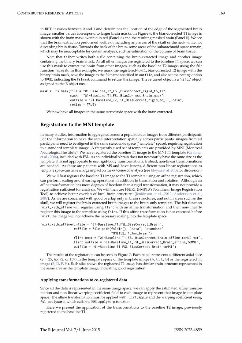
CONTRIBUTED RESEARCH ARTICLES 169
in BET: it varies between 0 and 1 and determines the location of the edge of the segmented brainimage; smaller values correspond to larger brain masks. In Figure 6, the bias-corrected T1 image isshown with the brain mask overlaid in red (Panel A) and the resulting masked brain (Panel B). We seethat the brain extraction performed well, not including any areas of the skull or the neck while notdiscarding brain tissue. Towards the back of the brain, some areas of the subarachnoid space remain,which may be unacceptable for certain analyses, such as estimation of the volume of brain tissue.
Note that fslbet writes both a file containing the brain-extracted image and another imagecontaining the binary brain mask. As all other images are registered to the baseline T1 space, we canuse this mask to extract the brain from other images, such as the baseline T2 image, using the fslrfunction fslmask. In this example, we mask the registered-to-T1, bias-corrected T2 image with thebinary brain mask, save the image to the filename specified in outfile, and also set the retimg optionto TRUE, indicating the fslmask command to return the image. The returned object is a ‘nifti’ object,assigned to the R object mask:
mask <- fslmask(file = "01-Baseline_T2_FSL_BiasCorrect_rigid_to_T1",mask = "01-Baseline_T1_FSL_BiasCorrect_Brain_mask",outfile = "01-Baseline_T2_FSL_BiasCorrect_rigid_to_T1_Brain",retimg = TRUE)
We now have all images in the same stereotaxic space with the brain extracted.
Registration to the MNI template
In many studies, information is aggregated across a population of images from different participants.For the information to have the same interpretation spatially across participants, images from allparticipants need to be aligned in the same stereotaxic space (“template” space), requiring registrationto a standard template image. A frequently used set of templates are provided by MNI (MontrealNeurological Institute). We have registered the baseline T1 image to the MNI T1 template (Grabneret al., 2006), included with FSL. As an individual’s brain does not necessarily have the same size as thetemplate, it is not appropriate to use rigid-body transformations. Instead, non-linear transformationsare needed. As these are patients with MS and have lesions, different non-linear registrations totemplate space can have a large impact on the outcome of analysis (see Eloyan et al. 2014 for discussion).
We will first register the baseline T1 image to the T1 template using an affine registration, whichcan perform scaling and shearing operations in addition to translation and rotation. Although anaffine transformation has more degrees of freedom than a rigid transformation, it may not provide aregistration sufficient for analysis. We will then use FNIRT (FMRIB’s Nonlinear Image RegistrationTool) to achieve better overlap of local brain structures (Jenkinson et al., 2012; Andersson et al.,2007). As we are concerned with good overlap only in brain structures, and not in areas such as theskull, we will register the brain-extracted brain images to the brain-only template. The fslr functionfnirt_with_affine will register using flirt with an affine transformation and then non-linearlyregister this image to the template using fnirt. If this affine transformation is not executed beforefnirt, the image will not achieve the necessary scaling into the template space.
fnirt_with_affine(infile = "01-Baseline_T1_FSL_BiasCorrect_Brain",reffile = file.path(fsldir(), "data", "standard",
"MNI152_T1_1mm_brain"),flirt.omat = "01-Baseline_T1_FSL_BiasCorrect_Brain_affine_toMNI.mat",flirt.outfile = "01-Baseline_T1_FSL_BiasCorrect_Brain_affine_toMNI",outfile = "01-Baseline_T1_FSL_BiasCorrect_Brain_toMNI")
The results of the registration can be seen in Figure 7. Each panel represents a different axial slice(z = 25, 45, 92, or 137) in the template space of the template image (A, C, E, G) or the registered T1image (B, D, F, H). Each slice shows the registered T1 image has similar brain structure represented inthe same area as the template image, indicating good registration.
Applying transformations to co-registered data
Since all the data is represented in the same image space, we can apply the estimated affine transfor-mation and non-linear warping coefficient field to each image to represent that image in templatespace. The affine transformation must be applied with flirt_apply and the warping coefficient usingfsl_applywarp, which calls the FSL applywarp function.
Here we present the application of the transformations to the baseline T2 image, previouslyregistered to the baseline T1.
The R Journal Vol. 7/1, June 2015 ISSN 2073-4859

CONTRIBUTED RESEARCH ARTICLES 170
Figure 7: Results from FNIRT. We present different axial slices of the template (A, C, E, G) and theregistered T1 image (B, D, F, H). The slices represented are 25 (A, B), 45 (C, D), 92 (E, F) and 137 (G, H).We note that areas of the brain coincide between the template and registered image.
flirt_apply(infile = "01-Baseline_T2_FSL_BiasCorrect_rigid_to_T1_Brain",reffile = file.path(fsldir(), "data", "standard", "MNI152_T1_1mm_brain"),initmat = "01-Baseline_T1_FSL_BiasCorrect_Brain_affine_toMNI.mat",outfile = "01-Baseline_T2_FSL_BiasCorrect_rigid_to_T1_Brain_toMNI")
fsl_applywarp(infile = "01-Baseline_T2_FSL_BiasCorrect_rigid_to_T1_Brain_toMNI",reffile = file.path(fsldir(), "data", "standard", "MNI152_T1_1mm_brain"),warpfile = "01-Baseline_T1_FSL_BiasCorrect_Brain_affine_toMNI_warpcoef",outfile = "01-Baseline_T2_FSL_BiasCorrect_rigid_to_T1_Brain_toMNI")
These two operations can also be performed in a single call to the fslr fnirt_with_affine_applyfunction.
With multiple participants, this process yields a multi-person, multi-modal, longitudinal imagingdataset that can be used for analyses.
Conclusion
The neuroimaging community has developed a large collection of tools for image processing andanalysis. R has a number of packages to perform operations on images; EBImage is one good example(Pau et al., 2010). Much of the fundamental functionality of neuroimage processing is not currentlyavailable in R, such as brain extraction and tissue segmentation. We present fslr to provide R usersfunctions for image processing and analysis that are based on FSL, an established image processingand analysis software suite. Interfacing R with existing, powerful software provides users withthoroughly-tested software and an additional community of users, which would not be available if thefunctions were rewritten in R. fslr should be easy to use for any standard R user; the workflow allowsR users to manipulate array-like ‘nifti’ objects, pass them to fslr functions, which return ‘nifti’objects. Moreover, as FSL and R are open-source and free, this software is readily available to all users.
There has been an increasing popularity of similar interfacing of tools within the Python commu-nity such as Nipype (Gorgolewski et al. 2011; https://qa.debian.org/popcon.php?package=nipype).As many users of R may not have experience with Python or bash scripting, we believe fslr provides alower threshold for use in the R community. Other packages provide R users additional neuroimagingprocessing functionality such as AnalyzeFMRI, RNiftyReg, and fmri.
For example, other inhomogeneity correction methods exist, such as the popular N3 (Sled et al.,1998) and N4 (Tustison et al., 2010), methods which are not implemented in fslr. ANTsR (Avantset al., 2015) is an R package that interfaces with the ANTs (advanced normalization tools) softwaresuite (Avants et al., 2011). ANTs has implementations of these correction methods, an increased set ofregistration techniques, and other methods for image processing. Other packages such as this, alongwith fslr, can create a diverse set of tools for neuroimaging within R, building on preexisting and
The R Journal Vol. 7/1, June 2015 ISSN 2073-4859
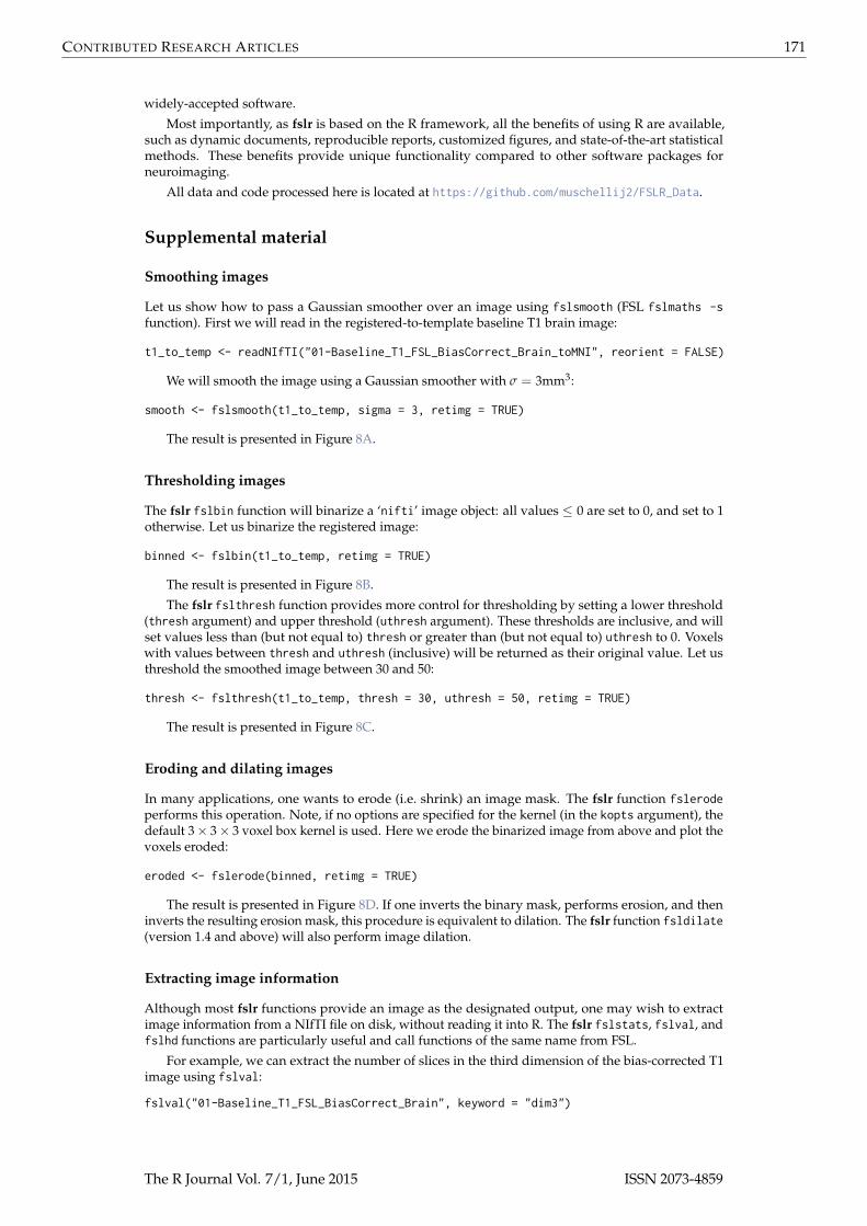
CONTRIBUTED RESEARCH ARTICLES 171
widely-accepted software.
Most importantly, as fslr is based on the R framework, all the benefits of using R are available,such as dynamic documents, reproducible reports, customized figures, and state-of-the-art statisticalmethods. These benefits provide unique functionality compared to other software packages forneuroimaging.
All data and code processed here is located at https://github.com/muschellij2/FSLR_Data.
Supplemental material
Smoothing images
Let us show how to pass a Gaussian smoother over an image using fslsmooth (FSL fslmaths -sfunction). First we will read in the registered-to-template baseline T1 brain image:
t1_to_temp <- readNIfTI("01-Baseline_T1_FSL_BiasCorrect_Brain_toMNI", reorient = FALSE)
We will smooth the image using a Gaussian smoother with σ = 3mm3:
smooth <- fslsmooth(t1_to_temp, sigma = 3, retimg = TRUE)
The result is presented in Figure 8A.
Thresholding images
The fslr fslbin function will binarize a ‘nifti’ image object: all values ≤ 0 are set to 0, and set to 1otherwise. Let us binarize the registered image:
binned <- fslbin(t1_to_temp, retimg = TRUE)
The result is presented in Figure 8B.
The fslr fslthresh function provides more control for thresholding by setting a lower threshold(thresh argument) and upper threshold (uthresh argument). These thresholds are inclusive, and willset values less than (but not equal to) thresh or greater than (but not equal to) uthresh to 0. Voxelswith values between thresh and uthresh (inclusive) will be returned as their original value. Let usthreshold the smoothed image between 30 and 50:
thresh <- fslthresh(t1_to_temp, thresh = 30, uthresh = 50, retimg = TRUE)
The result is presented in Figure 8C.
Eroding and dilating images
In many applications, one wants to erode (i.e. shrink) an image mask. The fslr function fslerodeperforms this operation. Note, if no options are specified for the kernel (in the kopts argument), thedefault 3× 3× 3 voxel box kernel is used. Here we erode the binarized image from above and plot thevoxels eroded:
eroded <- fslerode(binned, retimg = TRUE)
The result is presented in Figure 8D. If one inverts the binary mask, performs erosion, and theninverts the resulting erosion mask, this procedure is equivalent to dilation. The fslr function fsldilate(version 1.4 and above) will also perform image dilation.
Extracting image information
Although most fslr functions provide an image as the designated output, one may wish to extractimage information from a NIfTI file on disk, without reading it into R. The fslr fslstats, fslval, andfslhd functions are particularly useful and call functions of the same name from FSL.
For example, we can extract the number of slices in the third dimension of the bias-corrected T1image using fslval:
fslval("01-Baseline_T1_FSL_BiasCorrect_Brain", keyword = "dim3")
The R Journal Vol. 7/1, June 2015 ISSN 2073-4859
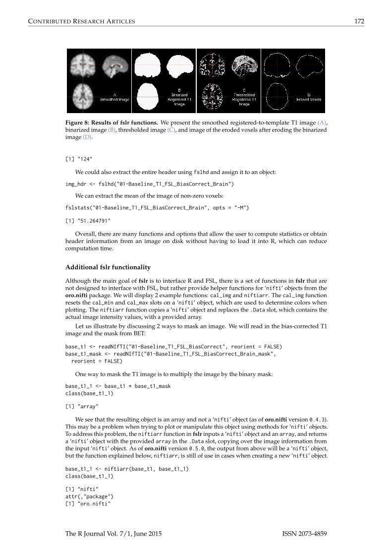
CONTRIBUTED RESEARCH ARTICLES 172
Figure 8: Results of fslr functions. We present the smoothed registered-to-template T1 image (A),binarized image (B), thresholded image (C), and image of the eroded voxels after eroding the binarizedimage (D).
[1] "124"
We could also extract the entire header using fslhd and assign it to an object:
img_hdr <- fslhd("01-Baseline_T1_FSL_BiasCorrect_Brain")
We can extract the mean of the image of non-zero voxels:
fslstats("01-Baseline_T1_FSL_BiasCorrect_Brain", opts = "-M")
[1] "51.264791"
Overall, there are many functions and options that allow the user to compute statistics or obtainheader information from an image on disk without having to load it into R, which can reducecomputation time.
Additional fslr functionality
Although the main goal of fslr is to interface R and FSL, there is a set of functions in fslr that arenot designed to interface with FSL, but rather provide helper functions for ‘nifti’ objects from theoro.nifti package. We will display 2 example functions: cal_img and niftiarr. The cal_img functionresets the cal_min and cal_max slots on a ‘nifti’ object, which are used to determine colors whenplotting. The niftiarr function copies a ‘nifti’ object and replaces the .Data slot, which contains theactual image intensity values, with a provided array.
Let us illustrate by discussing 2 ways to mask an image. We will read in the bias-corrected T1image and the mask from BET:
base_t1 <- readNIfTI("01-Baseline_T1_FSL_BiasCorrect", reorient = FALSE)base_t1_mask <- readNIfTI("01-Baseline_T1_FSL_BiasCorrect_Brain_mask",reorient = FALSE)
One way to mask the T1 image is to multiply the image by the binary mask:
base_t1_1 <- base_t1 * base_t1_maskclass(base_t1_1)
[1] "array"
We see that the resulting object is an array and not a ‘nifti’ object (as of oro.nifti version 0.4.3).This may be a problem when trying to plot or manipulate this object using methods for ‘nifti’ objects.To address this problem, the niftiarr function in fslr inputs a ‘nifti’ object and an array, and returnsa ‘nifti’ object with the provided array in the .Data slot, copying over the image information fromthe input ‘nifti’ object. As of oro.nifti version 0.5.0, the output from above will be a ‘nifti’ object,but the function explained below, niftiarr, is still of use in cases when creating a new ‘nifti’ object.
base_t1_1 <- niftiarr(base_t1, base_t1_1)class(base_t1_1)
[1] "nifti"attr(,"package")[1] "oro.nifti"
The R Journal Vol. 7/1, June 2015 ISSN 2073-4859
CONTRIBUTED RESEARCH ARTICLES 173
Another way of masking the image is to subset the values of the image that are not in the maskand setting those values to 0 (or some other value).
base_t1_2 <- base_t1base_t1_2[base_t1_mask == 0] <- 0class(base_t1_2)
[1] "nifti"attr(,"package")[1] "oro.nifti"
We see that this correctly returns an object of class ‘nifti’. One problem is that the we havechanged the data in the ‘nifti’ object base_t1_2 but did not reset the other slots in this object to reflectthis change.
In a ‘nifti’ object, the cal_min and cal_max slots equal the minimum and maximum values,respectively, of the data. The orthographic function (from oro.nifti) uses these values for plotting;also, if these slots do not equal the minimum and maximum, the writeNIfTI function (from oro.nifti)will fail. The cal_img is a simple helper function that will set the cal_min and cal_max slots to thecorrect values. Let us look at the range of the data and the cal_min and cal_max slots:
range(base_t1_2)
[1] 0.0000 409.3908
c(base_t1_2@cal_min, base_t1_2@cal_max)
[1] 0 0
An issue with the readNIfTI function from oro.nifti is that the cal_min and cal_max slots may be bothread as zero. Let us set these to the range using the cal_img command from fslr:
base_t1_2 <- cal_img(base_t1_2)c(base_t1_2@cal_min, base_t1_2@cal_max)
[1] 0.0000 409.3908
We see that after these operations are done in different ways, the resulting ‘nifti’ objects are equivalent.
identical(base_t1_1, base_t1_2)
[1] TRUE
Additional helper functions such as these are included in fslr for plotting and image manipulation.
Bibliography
J. L. Andersson, M. Jenkinson, and S. Smith. Non-linear registration, aka Spatial normalisation.FMRIB technical report TR07JA2, FMRIB Analysis Group of the University of Oxford, 2007. URLhttp://fmrib.medsci.ox.ac.uk/analysis/techrep/tr07ja2/tr07ja2.pdf. [p169]
J. Ashburner and K. J. Friston. Unified segmentation. NeuroImage, 26(3):839–851, 2005. [p167]
B. B. Avants, N. J. Tustison, G. Song, P. A. Cook, A. Klein, and J. C. Gee. A reproducible evaluation ofANTs similarity metric performance in brain image registration. NeuroImage, 54(3):2033–2044, Feb.2011. [p170]
B. B. Avants, B. M. Kandel, J. T. Duda, P. A. Cook, and N. J. Tustison. ANTsR: An R Package ProvidingANTs Features in R, 2015. URL http://stnava.github.io/ANTsR/. R package version 0.3.1. [p170]
C. Bordier, M. Dojat, and P. L. de Micheaux. Temporal and spatial independent component analysisfor fMRI data sets embedded in the AnalyzeFMRI R package. Journal of Statistical Software, 44(9):1–24, 2011. URL http://www.jstatsoft.org/v44/i09/. [p163]
J. Carp. The secret lives of experiments: Methods reporting in the fMRI literature. NeuroImage, 63(1):289–300, Oct. 2012. [p163]
J. Clayden. RNiftyReg: Medical Image Registration Using the NiftyReg Library, 2015. URL http://CRAN.R-project.org/package=RNiftyReg. R package version 1.1.3, based on original code by Marc Modatand Pankaj Daga. [p163]
The R Journal Vol. 7/1, June 2015 ISSN 2073-4859
CONTRIBUTED RESEARCH ARTICLES 174
R. W. Cox. AFNI: Software for analysis and visualization of functional magnetic resonance neuroim-ages. Computers and Biomedical Research, 29(3):162–173, 1996. [p167]
J. Doshi, G. Erus, Y. Ou, B. Gaonkar, and C. Davatzikos. Multi-atlas skull-stripping. Academic Radiology,20(12):1566–1576, Dec. 2013. [p167]
A. Eloyan, H. Shou, R. T. Shinohara, E. M. Sweeney, M. B. Nebel, J. L. Cuzzocreo, P. A. Calabresi, D. S.Reich, M. A. Lindquist, and C. M. Crainiceanu. Health effects of lesion localization in multiplesclerosis: Spatial registration and confounding adjustment. PLoS ONE, 9(9):e107263, Sept. 2014.[p169]
B. Fischl. FreeSurfer. NeuroImage, 62(2):774–781, 2012. [p167]
K. Gorgolewski, C. D. Burns, C. Madison, D. Clark, Y. O. Halchenko, M. L. Waskom, and S. S. Ghosh.Nipype: A flexible, lightweight and extensible neuroimaging data processing framework in Python.Frontiers in Neuroinformatics, 5(13), 2011. [p170]
G. Grabner, A. L. Janke, M. M. Budge, D. Smith, J. Pruessner, and D. L. Collins. Symmetric atlasing andmodel based segmentation: An application to the hippocampus in older adults. In D. Hutchison,T. Kanade, J. Kittler, J. M. Kleinberg, F. Mattern, J. C. Mitchell, M. Naor, O. Nierstrasz, C. P. Rangan,B. Steffen, M. Sudan, D. Terzopoulos, D. Tygar, M. Y. Vardi, G. Weikum, R. Larsen, M. Nielsen, andJ. Sporring, editors, Medical Image Computing and Computer-Assisted Intervention – MICCAI 2006,volume 4191, pages 58–66. Springer Berlin Heidelberg, Berlin, Heidelberg, 2006. [p169]
R. Guillemaud and M. Brady. Estimating the bias field of MR images. IEEE Transactions on MedicalImaging, 16(3):238–251, 1997. [p164]
T. J. Hastie and R. J. Tibshirani. Generalized Additive Models, volume 43. CRC Press, 1990. [p164]
M. Jenkinson and S. Smith. A global optimisation method for robust affine registration of brain images.Medical Image Analysis, 5(2):143–156, 2001. [p163, 165]
M. Jenkinson, P. Bannister, M. Brady, and S. Smith. Improved optimization for the robust and accuratelinear registration and motion correction of brain images. NeuroImage, 17(2):825–841, 2002. [p163,165]
M. Jenkinson, M. Pechaud, and S. Smith. BET2: MR-based estimation of brain, skull and scalp surfaces.In Eleventh Annual Meeting of the Organization for Human Brain Mapping, volume 17, 2005. URLhttp://mickaelpechaud.free.fr/these/HBM05.pdf. [p167]
M. Jenkinson, C. F. Beckmann, T. E. J. Behrens, M. W. Woolrich, and S. M. Smith. FSL. NeuroImage, 62(2):782–790, Aug. 2012. [p163, 169]
G. Pau, F. Fuchs, O. Sklyar, M. Boutros, and W. Huber. EBImage—an R package for image processingwith applications to cellular phenotypes. Bioinformatics, 26(7):979–981, 2010. [p170]
V. Popescu, M. Battaglini, W. S. Hoogstrate, S. C. J. Verfaillie, I. C. Sluimer, R. A. van Schijndel,B. W. van Dijk, K. S. Cover, D. L. Knol, M. Jenkinson, F. Barkhof, N. de Stefano, and H. Vrenken.Optimizing parameter choice for FSL-Brain Extraction Tool (BET) on 3d T1 images in multiplesclerosis. NeuroImage, 61(4):1484–1494, July 2012. [p167]
J. G. Sled, A. P. Zijdenbos, and A. C. Evans. A nonparametric method for automatic correction ofintensity nonuniformity in MRI data. IEEE Transactions on Medical Imaging, 17(1):87–97, 1998. [p170]
S. M. Smith. Fast robust automated brain extraction. Human Brain Mapping, 17(3):143–155, Nov. 2002.[p163, 167]
E. M. Sweeney, R. T. Shinohara, C. D. Shea, D. S. Reich, and C. M. Crainiceanu. Automatic lesionincidence estimation and detection in multiple sclerosis using multisequence longitudinal MRI.American Journal of Neuroradiology, 34(1):68–73, Jan. 2013. [p164]
K. Tabelow and J. Polzehl. Statistical parametric maps for functional MRI experiments in R: Thepackage fmri. Journal of Statistical Software, 44(11):1–21, 2011. URL http://www.jstatsoft.org/v44/i11/. [p163]
N. J. Tustison, B. B. Avants, P. A. Cook, Y. Zheng, A. Egan, P. A. Yushkevich, and J. C. Gee. N4itk:Improved N3 bias correction. IEEE Transactions on Medical Imaging, 29(6):1310–1320, 2010. [p170]
B. Whitcher, V. J. Schmid, and A. Thornton. Working with the DICOM and NIfTI data standards in R.Journal of Statistical Software, 44(6):1–28, 2011. URL http://www.jstatsoft.org/v44/i06/. [p163]
The R Journal Vol. 7/1, June 2015 ISSN 2073-4859

CONTRIBUTED RESEARCH ARTICLES 175
H. Wickham. ggplot2: Elegant Graphics for Data Analysis. Springer, 2009. URL http://had.co.nz/ggplot2/book. [p164]
S. N. Wood. Fast stable restricted maximum likelihood and marginal likelihood estimation of semi-parametric generalized linear models. Journal of the Royal Statistical Society: Series B (StatisticalMethodology), 73(1):3–36, 2011. [p164]
Y. Zhang, M. Brady, and S. Smith. Segmentation of brain MR images through a hidden Markov randomfield model and the expectation-maximization algorithm. IEEE Transactions on Medical Imaging, 20(1):45–57, 2001. [p163, 164]
John MuschelliPhD StudentJohns Hopkins Bloomberg School of Public Health,Baltimore, MD [email protected]
Elizabeth SweeneyPhD StudentJohns Hopkins Bloomberg School of Public Health,Baltimore, MD 21231USASpecial Volunteer Translational Neuroradiology Unit, Neuroimmunology Branch, National Institute of Neuro-logical Disease and Stroke, National Institute of Health,Bethesda, MD [email protected]
Martin LindquistAssociate ProfessorJohns Hopkins Bloomberg School of Public Health,Baltimore, MD [email protected]
Ciprian CrainiceanuProfessorJohns Hopkins Bloomberg School of Public Health,Baltimore, MD [email protected]
The R Journal Vol. 7/1, June 2015 ISSN 2073-4859