FROM VERTICES TO

FRAGMENTS

Basic Implementation Strategies

In computer graphics, we start with an application program,

and we end with an image.

We can consider this process as a black box whose inputs are

the vertices and states defined in the program geometric

objects, attributes, camera specifications and whose output is

an array of colored pixels in the frame buffer

Basic Implementation Strategies

Within the black box, we must do many tasks, including

transformations, clipping, shading, hidden-surface removal, and

rasterization of the primitives that can appear on the display.

These tasks can be organized in a variety of ways, but regardless

of the strategy that we adopt, we must always do two things:

1.We must pass every geometric object through the system,

2.We must assign a color to every pixel in the color buffer that is

displayed

Basic Implementation Strategies

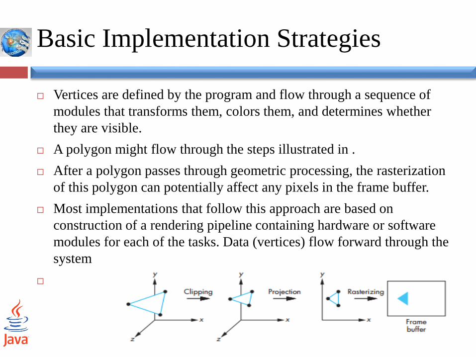
Vertices are defined by the program and flow through a sequence of

modules that transforms them, colors them, and determines whether

they are visible.

A polygon might flow through the steps illustrated in .

After a polygon passes through geometric processing, the rasterization

of this polygon can potentially affect any pixels in the frame buffer.

Most implementations that follow this approach are based on

construction of a rendering pipeline containing hardware or software

modules for each of the tasks. Data (vertices) flow forward through the

system

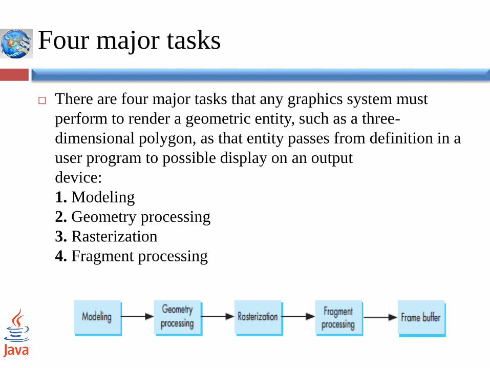
Four major tasks

There are four major tasks that any graphics system must

perform to render a geometric entity, such as a three-

dimensional polygon, as that entity passes from definition in a

user program to possible display on an output

device:

1. Modeling

2. Geometry processing

3. Rasterization

4. Fragment processing

1.Modeling

The usual results of the modeling process are sets of vertices

that specify a group of geometric objects supported by the rest

of the system.

We can look at the modeler as a black box that produces

geometric objects and is usually a user program.

1.Modeling con…

There are other tasks that the modeler might perform.

Consider, for example, clipping: the process of eliminating parts of

objects that cannot appear on the display because they lie outside

the viewing volume.

A user can generate geometric objects in her program, and she can

hope that the rest of the system can process these objects at the rate

at which they are produced, or the modeler can attempt to ease the

burden on the rest of the system by minimizing the number of

objects that it passes on.

The modeler may do some of the same jobs as the rest of the system

.

2.Geometry Processing

Geometry processing works with vertices.

The goals of the geometry processor are to determine which

geometric objects can appear on the display and to assign

shades or colors to the vertices of these objects.

Four processes are required:

projection, primitive assembly, clipping, and shading

2.Geometry Processing con…

Geometric objects are transformed by a sequence of

transformations that may reshape and move them (modeling)

or may change their representations (viewing).

View volume

Those primitives that fit within a specified volume, can appear

on the display after rasterization.

Primitive assembly

The process of grouping vertices into objects before clipping

can take place.

2.Geometry Processing con..

hidden-surface removal

Note that even though an object lies inside the view volume, it

will not be visible if it is obscured by other objects.

Algorithms for hidden-surface removal or visible-surface

determination are based on the three-dimensional spatial

relationships among objects.

This step is normally carried out as part of fragment

processing.

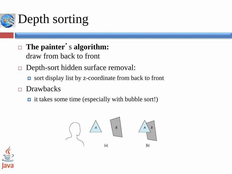
Depth sorting

The painter’s algorithm:

draw from back to front

Depth-sort hidden surface removal:

sort display list by z-coordinate from back to front

Drawbacks

it takes some time (especially with bubble sort!)

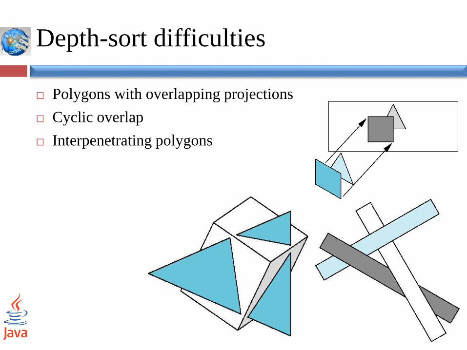
Depth-sort difficulties

Polygons with overlapping projections

Cyclic overlap

Interpenetrating polygons

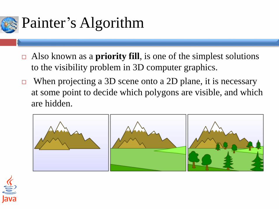
Painter’s Algorithm13

Also known as a priority fill, is one of the simplest solutions

to the visibility problem in 3D computer graphics.

When projecting a 3D scene onto a 2D plane, it is necessary

at some point to decide which polygons are visible, and which

are hidden.

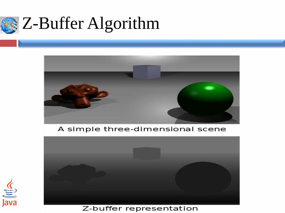
Z-Buffer Algorithm 14

z-buffering, also known as depth buffering, is the management of

image depth coordinates in three-dimensional (3-D) graphics.

It is one solution to the visibility problem, which is the problem of

deciding which elements of a rendered scene are visible, and which

are hidden.

When an object is rendered, the depth of a generated pixel (z

coordinate) is stored in a buffer (the z-buffer or depth buffer).

This buffer is usually arranged as a two-dimensional array (x-y)

with one element for each screen pixel. If another object of the

scene must be rendered in the same pixel, the method compares the

two depths and chooses the one closer to the observer.

Z-Buffer Algorithm

3.Rasterisation

Rasterisation is the task of taking an image described in a

vector graphics format (shapes) and converting it into a raster

image (pixels or dots) for output on a video display or printer,

or for storage in a bitmap file format .

It the transformation of geometric primitives (line segments,

circles, polygons) into a raster image representation, i. e. pixel

positions the estimation of an appropriate set of pixel

positions to represent a geometric primitive.

4.Fragment Processing

In the simplest situations, each fragment is assigned a color by

the rasterizer and this color is placed in the frame buffer at the

locations corresponding to the fragment’s location.

Objects that are in the view volume will not be visible if they

are blocked by any opaque objects closer to the viewer.

The required hidden-surface removal process is typically

carried out on a fragment-by-fragment basis.

4.Fragment Processing con..

In most displays, the process of taking the image from the

frame buffer and displaying it on a monitor happens

automatically and is not of concern to the application

program.

There are numerous problems with the quality of display, such

as the jaggedness or aliasing associated with images on raster

displays.

Clipping

Clipping is the process of determining which primitives, or

parts of primitives, fit within the clipping or view volume

defined by the application program.

We shall concentrate on clipping of line segments and

polygons because they are the most common primitives to

pass down the pipeline

Line segment clipping

A clipper decides which primitives, or parts of primitives, can

possibly appear on the display and be passed on to the

rasterizer.

Primitives that fit within the specified view volume pass

through the clipper, or are accepted.

Primitives that cannot appear on the display are eliminated, or

rejected or culled.

Primitives that are only partially within the view volume must

be clipped such that any part lying outside the volume is

removed

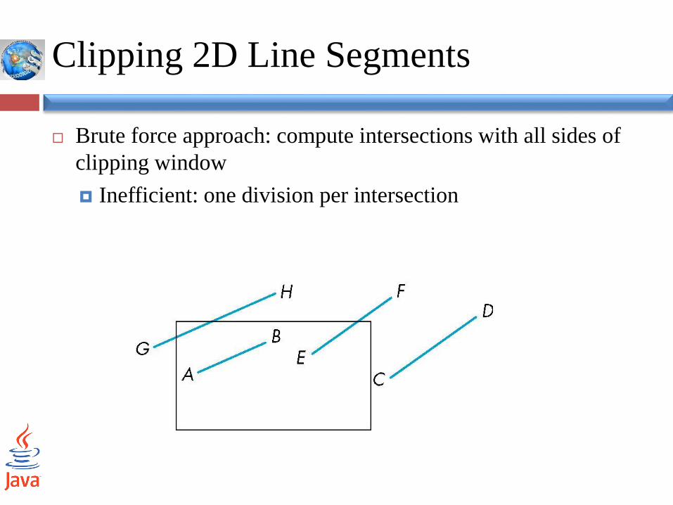
Clipping 2D Line Segments

Brute force approach: compute intersections with all sides of

clipping window

Inefficient: one division per intersection

Line Clipping

Line clipping operations should comprise the following cases:

Totally plotted.

Partially plotted.

Not plotted at all

Line Clipping con…

Note that even though neither of two vertices is within the

window , certain part of the line segment may be still within .

There are many different techniques for clipping line in 2D:

The fundamental are :

1-Line equation

2-Intersection computation

Next we will discuss Cohen-Sutherland Algorithm.

Cohen-Sutherland Algorithm

It is not the most efficient algorithm .

It is the most commonly used .

The key technique is 4 bit code

TBRL where:

T is set (to 1 ) if y > top

B is set (to 1 ) if y < Bottom

R is set (to 1 ) if x > right

L is set (to 1 ) if x < left

Cohen-Sutherland Algorithm con…

25

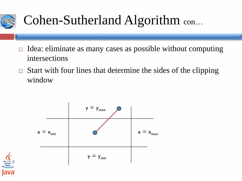
Idea: eliminate as many cases as possible without computing

intersections

Start with four lines that determine the sides of the clipping

window

x = xmaxx = xmin

y = ymax

y = ymin

The Cases26

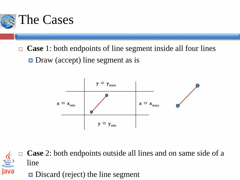
Case 1: both endpoints of line segment inside all four lines

Draw (accept) line segment as is

Case 2: both endpoints outside all lines and on same side of a

line

Discard (reject) the line segment

x = xmaxx = xmin

y = ymax

y = ymin

The Cases con…

27

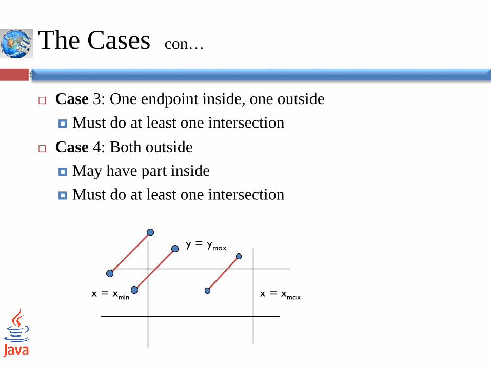
Case 3: One endpoint inside, one outside

Must do at least one intersection

Case 4: Both outside

May have part inside

Must do at least one intersection

x = xmaxx = xmin

y = ymax

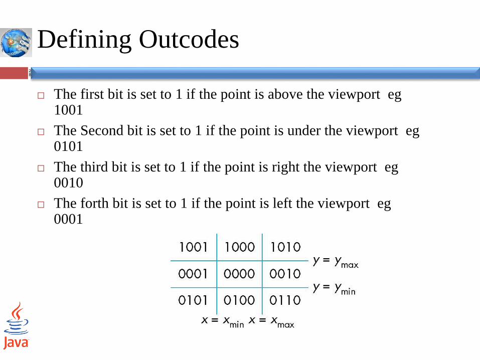
Defining Outcodes28

The first bit is set to 1 if the point is above the viewport eg1001

The Second bit is set to 1 if the point is under the viewport eg0101

The third bit is set to 1 if the point is right the viewport eg0010

The forth bit is set to 1 if the point is left the viewport eg0001

Using Outcodes29

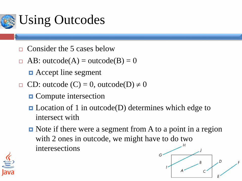
Consider the 5 cases below

AB: outcode(A) = outcode(B) = 0

Accept line segment

CD: outcode (C) = 0, outcode(D) 0

Compute intersection

Location of 1 in outcode(D) determines which edge to

intersect with

Note if there were a segment from A to a point in a region

with 2 ones in outcode, we might have to do two

interesections

Using Outcodes con…

30

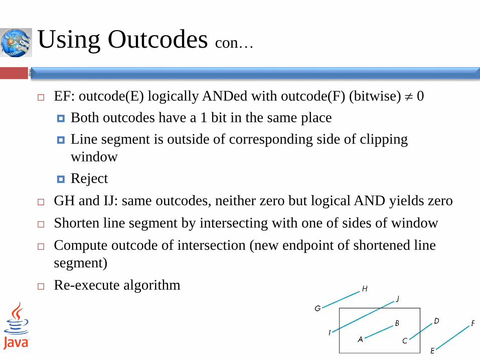
EF: outcode(E) logically ANDed with outcode(F) (bitwise) 0

Both outcodes have a 1 bit in the same place

Line segment is outside of corresponding side of clipping

window

Reject

GH and IJ: same outcodes, neither zero but logical AND yields zero

Shorten line segment by intersecting with one of sides of window

Compute outcode of intersection (new endpoint of shortened line

segment)

Re-execute algorithm

Efficiency31

In many applications, the clipping window is small relative to

the size of the entire data base

Most line segments are outside one or more sides of the

window and can be eliminated based on their outcodes

Inefficiency when code has to be re-executed for line

segments that must be shortened in more than one step

Polygon Clipping 32

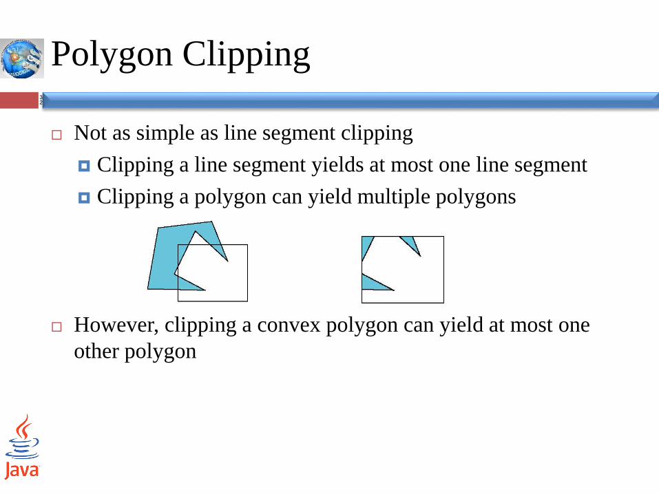
Not as simple as line segment clipping

Clipping a line segment yields at most one line segment

Clipping a polygon can yield multiple polygons

However, clipping a convex polygon can yield at most one

other polygon

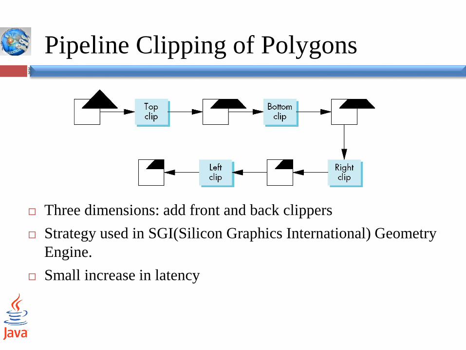
Pipeline Clipping of Polygons33

Three dimensions: add front and back clippers

Strategy used in SGI(Silicon Graphics International) Geometry

Engine.

Small increase in latency

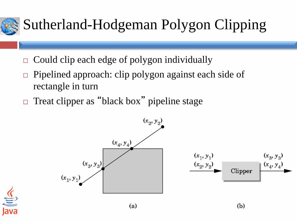
Sutherland-Hodgeman Polygon Clipping

Could clip each edge of polygon individually

Pipelined approach: clip polygon against each side of

rectangle in turn

Treat clipper as “black box” pipeline stage

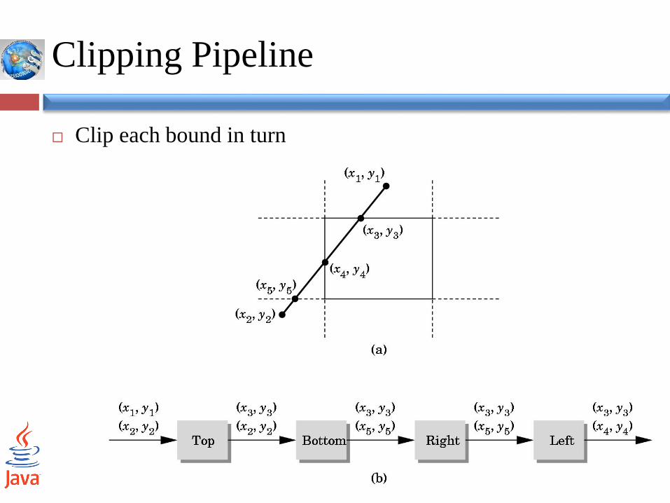
Clipping Pipeline

Clip each bound in turn

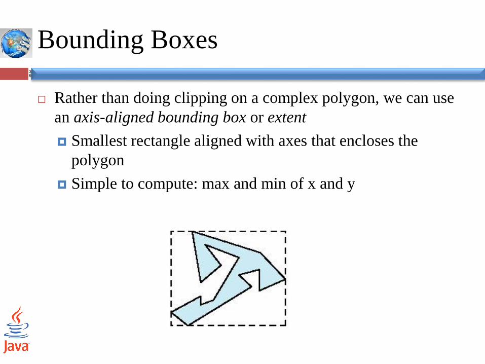
Bounding Boxes36

Rather than doing clipping on a complex polygon, we can use

an axis-aligned bounding box or extent

Smallest rectangle aligned with axes that encloses the

polygon

Simple to compute: max and min of x and y

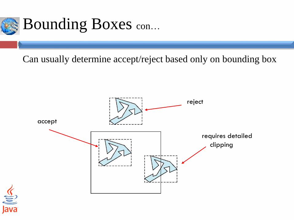
Bounding Boxes con…

37

Can usually determine accept/reject based only on bounding box

reject

accept

requires detailed

clipping

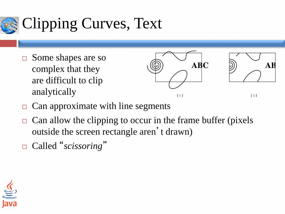
Clipping Curves, Text

Some shapes are so

complex that they

are difficult to clip

analytically

Can approximate with line segments

Can allow the clipping to occur in the frame buffer (pixels

outside the screen rectangle aren’t drawn)

Called “scissoring”

What is Scan conversion?

Final step of rasterization (the process of taking geometric

shapes and converting them into array of pixels stored in the

frame buffer to be displayed )

Take place after clipping accurs .

All graphics package do this at end of rendering pipeline

Take triangles and maps them to pixels on the screen

Also take into account other properties like lighting and

shading ,but we will focus on first on algorithm for line scan

conversion.

Design criteria of straight lines

What is the key issues of drawing a line ?

Find the addressable pixels which most closely approximate

this line .

Straight line should appear straight .

Line should start and end accurately matching end points with

connecting lines.

Lines should have constant brightness.

Lines should be drawn as rapidly as possible.

Design criteria of straight lines con...

Problem

Others create problems:

Stair casing

Aliasing

Quality of the line depend on the location of the pixels and

their brightness.

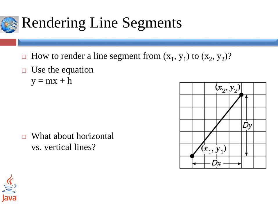
Rendering Line Segments

How to render a line segment from (x1, y1) to (x2, y2)?

Use the equation

y = mx + h

What about horizontal

vs. vertical lines?

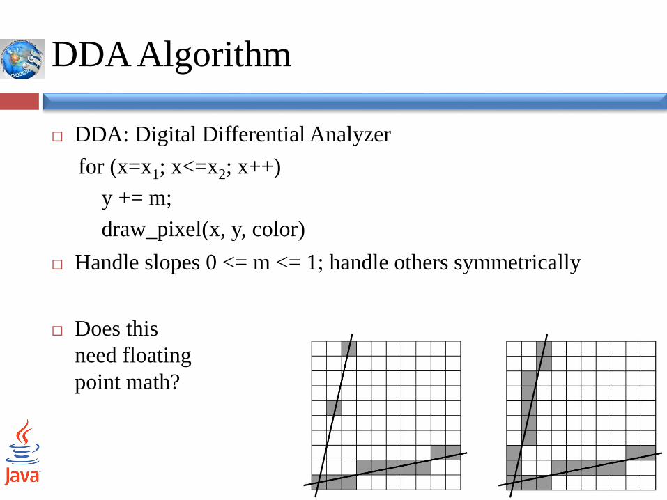
DDA Algorithm

DDA: Digital Differential Analyzer

for (x=x1; x<=x2; x++)

y += m;

draw_pixel(x, y, color)

Handle slopes 0 <= m <= 1; handle others symmetrically

Does this

need floating

point math?

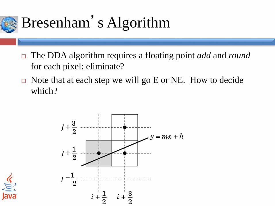
Bresenham’s Algorithm

The DDA algorithm requires a floating point add and round

for each pixel: eliminate?

Note that at each step we will go E or NE. How to decide

which?

−

Bresenham Decision Variable

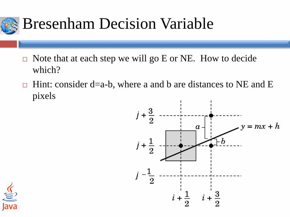
Note that at each step we will go E or NE. How to decide

which?

Hint: consider d=a-b, where a and b are distances to NE and E

pixels

−

Bresenham Decision Variable con…

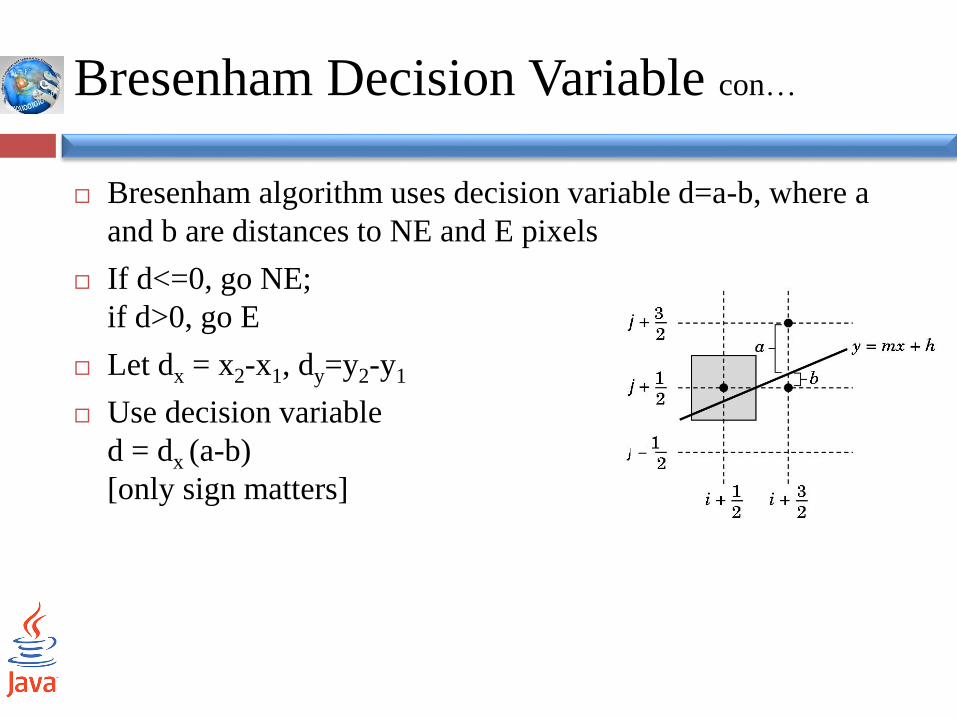
Bresenham algorithm uses decision variable d=a-b, where a

and b are distances to NE and E pixels

If d<=0, go NE;

if d>0, go E

Let dx = x2-x1, dy=y2-y1

Use decision variable

d = dx (a-b)

[only sign matters]

−

Bresenham Decision Variable

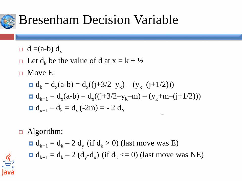
d =(a-b) dx

Let dk be the value of d at x = k + ½

Move E:

dk = dx(a-b) = dx((j+3/2–yk) – (yk–(j+1/2)))

dk+1 = dx(a-b) = dx((j+3/2–yk–m) – (yk+m–(j+1/2)))

dx+1 – dk = dx (-2m) = - 2 dY

Algorithm:

dk+1 = dk – 2 dy (if dk > 0) (last move was E)

dk+1 = dk – 2 (dy-dx) (if dk <= 0) (last move was NE)

−

Bresenham’s Algorithm

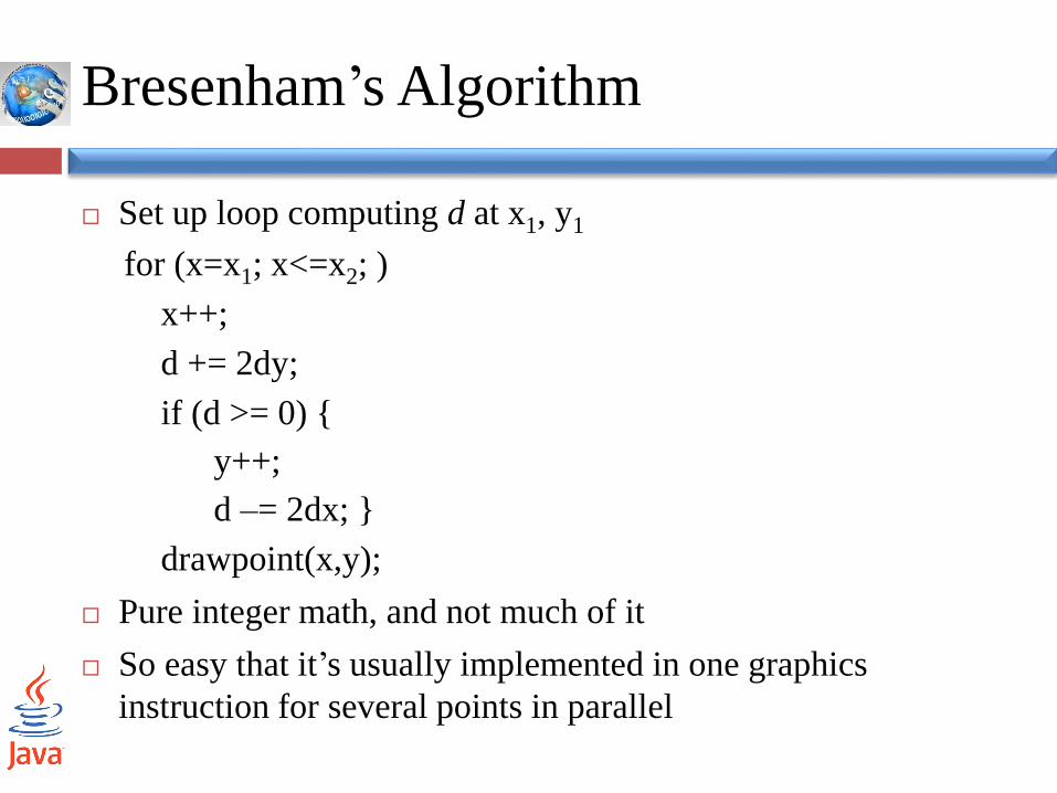
Set up loop computing d at x1, y1

for (x=x1; x<=x2; )

x++;

d += 2dy;

if (d >= 0) {

y++;

d –= 2dx; }

drawpoint(x,y);

Pure integer math, and not much of it

So easy that it’s usually implemented in one graphics

instruction for several points in parallel

Polygons Rasterization

Flat simple polygons have well-defined interiors. If they are

also convex, they are guaranteed to be rendered correctly by

OpenGL and by other graphics systems.

For nonflat polygons, we can work with their projections, or

we can use the first three vertices to determine a plane to use

for the interior.

For flat nonsimple polygons, we must decide how to

determine whether a given point is inside or outside of the

polygon.

Polygons Rasterization con…

The process of filling the inside of a polygon with a color or pattern

is equivalent to deciding which points in the plane of the polygon

are interior (inside) points.

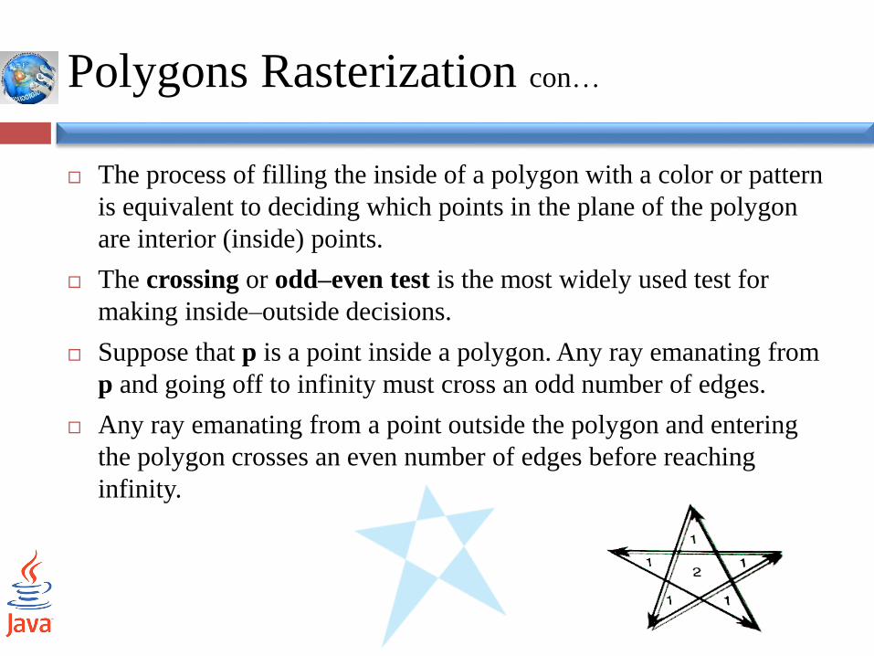
The crossing or odd–even test is the most widely used test for

making inside–outside decisions.

Suppose that p is a point inside a polygon. Any ray emanating from

p and going off to infinity must cross an odd number of edges.

Any ray emanating from a point outside the polygon and entering

the polygon crosses an even number of edges before reaching

infinity.

Polygons Rasterization con…

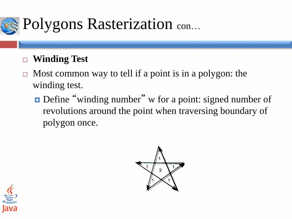
Winding Test

Most common way to tell if a point is in a polygon: the

winding test.

Define “winding number” w for a point: signed number of

revolutions around the point when traversing boundary of

polygon once.

Aliasing

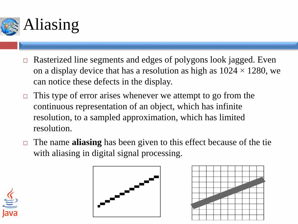
Rasterized line segments and edges of polygons look jagged. Even

on a display device that has a resolution as high as 1024 × 1280, we

can notice these defects in the display.

This type of error arises whenever we attempt to go from the

continuous representation of an object, which has infinite

resolution, to a sampled approximation, which has limited

resolution.

The name aliasing has been given to this effect because of the tie

with aliasing in digital signal processing.

Anti-Aliasing

Simplest approach: area-based weighting

Fastest approach: averaging nearby pixels

Most common approach: supersampling (compute four values

per pixel and avg, e.g.)

Best approach: weighting based on distance of pixel from

center of line; Gaussian fall-off

Temporal Aliasing

Need motion blur for motion that doesn’t flicker

Common approach: temporal supersampling

render images at several times within frame time interval

average results

Display Considerations

Color systems

Color quantization

Gamma correction

Dithering and Halftoning

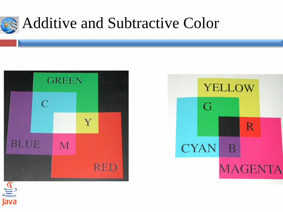
Additive and Subtractive Color

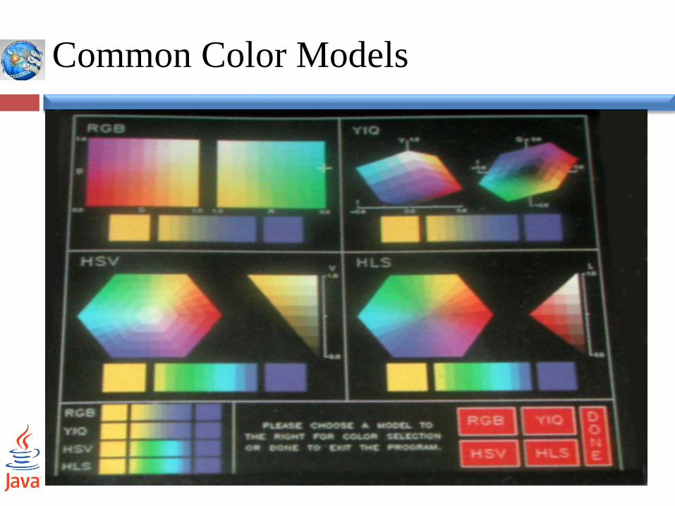
Common Color Models

Color Systems

RGB

YIQ

CMYK

HSV, HLS

Chromaticity

Color gamut

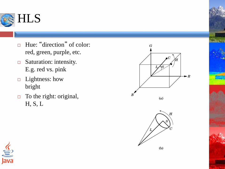
HLS

Hue: “direction” of color:

red, green, purple, etc.

Saturation: intensity.

E.g. red vs. pink

Lightness: how

bright

To the right: original,

H, S, L

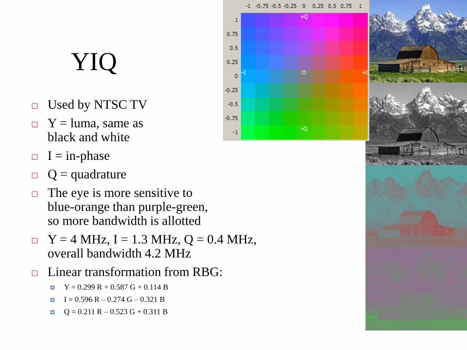
YIQ

Used by NTSC TV

Y = luma, same as black and white

I = in-phase

Q = quadrature

The eye is more sensitive to blue-orange than purple-green,so more bandwidth is allotted

Y = 4 MHz, I = 1.3 MHz, Q = 0.4 MHz, overall bandwidth 4.2 MHz

Linear transformation from RBG: Y = 0.299 R + 0.587 G + 0.114 B

I = 0.596 R – 0.274 G – 0.321 B

Q = 0.211 R – 0.523 G + 0.311 B

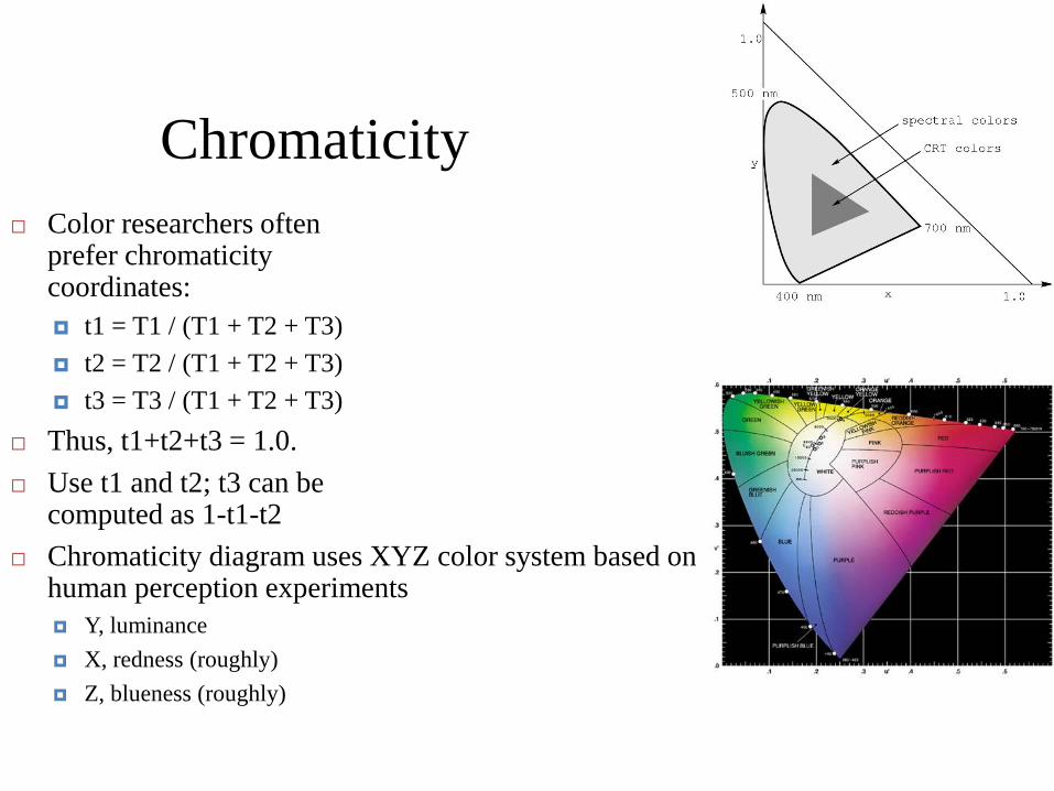
Chromaticity

Color researchers often prefer chromaticity coordinates:

t1 = T1 / (T1 + T2 + T3)

t2 = T2 / (T1 + T2 + T3)

t3 = T3 / (T1 + T2 + T3)

Thus, t1+t2+t3 = 1.0.

Use t1 and t2; t3 can be computed as 1-t1-t2

Chromaticity diagram uses XYZ color system based on human perception experiments

Y, luminance

X, redness (roughly)

Z, blueness (roughly)

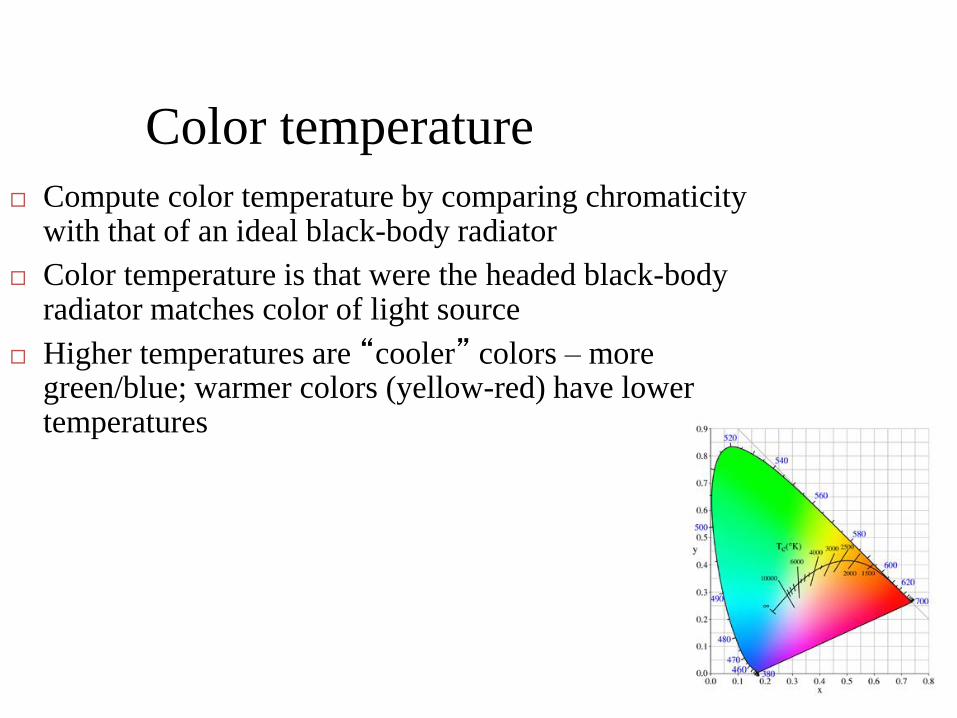
Color temperature

Compute color temperature by comparing chromaticity with that of an ideal black-body radiator

Color temperature is that were the headed black-body radiator matches color of light source

Higher temperatures are “cooler” colors – more green/blue; warmer colors (yellow-red) have lower temperatures

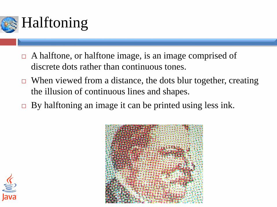
Halftoning

A halftone, or halftone image, is an image comprised of

discrete dots rather than continuous tones.

When viewed from a distance, the dots blur together, creating

the illusion of continuous lines and shapes.

By halftoning an image it can be printed using less ink.

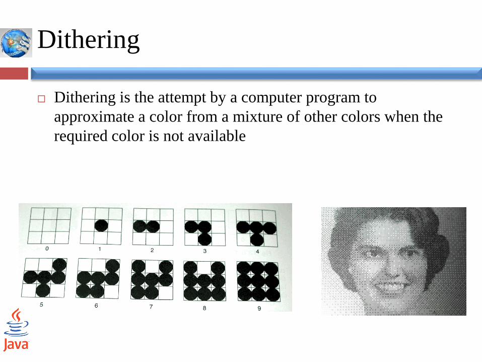
Dithering

Dithering is the attempt by a computer program to

approximate a color from a mixture of other colors when the

required color is not available

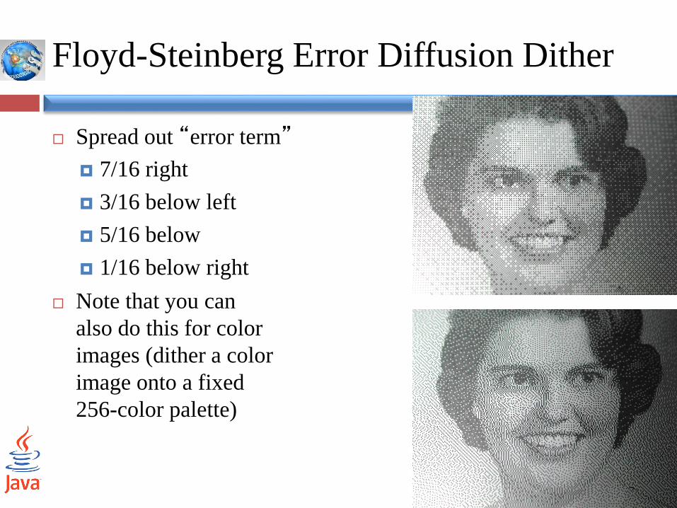
Floyd-Steinberg Error Diffusion Dither

Spread out “error term”

7/16 right

3/16 below left

5/16 below

1/16 below right

Note that you can

also do this for color

images (dither a color

image onto a fixed

256-color palette)