Freezing traveling and rotating waves insecond order evolution equations

Wolf-Jürgen Beyn, Denny Otten,Jens Rottmann-Matthes

CRC Preprint 2016/36, November 2016

KARLSRUHE INSTITUTE OF TECHNOLOGY

KIT – The Research University in the Helmholtz Association www.kit.edu

Participating universities

Funded by

ISSN 2365-662X

2

Freezing Traveling and Rotating Wavesin Second Order Evolution Equations

Wolf-Jürgen Beyn1,4

Denny Otten2,4

Department of MathematicsBielefeld University33501 BielefeldGermany

Jens Rottmann-Matthes3,5

Institut für AnalysisKarlsruhe Institute of Technology76131 KarlsruheGermany

Date: November 28, 2016

Abstract. In this paper we investigate the implementation of the so-called freezing method for secondorder wave equations in one and several space dimensions. The method converts the given PDE intoa partial differential algebraic equation which is then solved numerically. The reformulation aims atseparating the motion of a solution into a co-moving frame and a profile which varies as little as possible.Numerical examples demonstrate the feasability of this approach for semilinear wave equations withsufficient damping. We treat the case of a traveling wave in one space dimension and of a rotating wavein two space dimensions. In addition, we investigate in arbitrary space dimensions the point spectrumand the essential spectrum of operators obtained by linearizing about the profile, and we indicate theconsequences for the nonlinear stability of the wave.

Key words. Systems of damped wave equations, traveling waves, rotating waves, freezing method, secondorder evolution equations, point spectra, essential spectra.AMS subject classification. 35K57, 35Pxx, 65Mxx (35Q56, 47N40, 65P40).

1. IntroductionThe topic of this paper is the numerical computation and stability of waves occurring in second orderevolution equations with damping terms. More specifically, we transfer the so called freezing method(see [7], [19], [4]) from first order to second order evolution equations, and we investigate its relation tothe stability of the waves. Generally speaking, the method tries to separate the solution of a Cauchyproblem into the motion of a co-moving frame and of a profile, where the latter is required to vary aslittle as possible or even become stationary. This is achieved by transforming the original PDE into apartial differential algebraic equation (PDAE). The PDAE involves extra unknowns specifying the frame,and extra constraints (so called phase conditions) enforcing the freezing principle for the profile. Thismethodology has been successfully applied to a wide range of PDEs which are of first order in time andof hyperbolic, parabolic or of mixed type, cf. [21], [23], [22], [6], [16], [17], [18], [4]. One aim of thetheoretical underpinning is to prove that waves which are (asymptotically) stable with asymptotic phasefor the PDE, become stable in the classical Lyapunov sense for the PDAE. While this has been rigorouslyproved for many systems in one space dimension and confirmed numerically in higher space dimensions,the corresponding theory for the multi-dimensional case is still in its early stages, see [1], [3], [2], [14].

1e-mail: beyn@math.uni-bielefeld.de, phone: +49 (0)521 106 4798,fax: +49 (0)521 106 6498, homepage: http://www.math.uni-bielefeld.de/~beyn/AG_Numerik/.

2e-mail: dotten@math.uni-bielefeld.de, phone: +49 (0)521 106 4784,fax: +49 (0)521 106 6498, homepage: http://www.math.uni-bielefeld.de/~dotten/.

3e-mail: jens.rottmann-matthes@kit.edu, phone: +49 (0)721 608 41632,fax: +49 (0)721 608 46530, homepage: http://www.math.kit.edu/iana2/~rottmann/.

4supported by CRC 701 ’Spectral Structures and Topological Methods in Mathematics’, Bielefeld University5supported by CRC 1173 ’Wave Phenomena: Analysis and Numerics’, Karlsruhe Institute of Technology

1

2

In this paper we develop the freezing formulation and perform the spectral calculations in an informalway, for the one-dimensional as well as the multi-dimensional case. Rigorous stability results for theone-dimensional damped wave equation may be found in [10], [9], [5].Here we consider a nonlinear wave equation of the form

(1.1) Mutt = Auxx + f(u, ux, ut), x ∈ R, t > 0,

where u(x, t) ∈ Rm, A,M ∈ Rm,m and f : R3m → Rm is sufficiently smooth. In addition, we assume thematrixM to be nonsingular andM−1A to be positive diagonalizable, which will lead to local wellposednessof the Cauchy problem associated with (1.1). Our interest is in traveling waves

u?(x, t) = v?(x− µ?t), x ∈ R, t > 0,

with constant limits at ±∞, i.e.

(1.2) limξ→±∞

v?(ξ) = v± ∈ Rm, limξ→±∞

v?,ξ(ξ) = 0, f(v±, 0, 0) = 0.

Transforming (1.1) into a co-moving frame via u(x, t) = v(ξ, t), ξ = x− µ?t leads to the system

(1.3) Mvtt = (A− µ2?M)vξξ + 2µ?Mvξt + f(v, vξ, vt − µ?vξ), ξ ∈ R, t > 0.

This system has v? as a steady state,

(1.4) 0 = (A− µ2?M)v?,ξξ + f(v?, v?,ξ,−µ?v?,ξ), ξ ∈ R.

In Section 2 we work out the details of the freezing PDAE based on the ansatz u(x, t) = v(x − γ(t), t),x ∈ R, t ≥ 0 with the additional unknown function γ(t), t ≥ 0. Solving this PDAE numerically will then bedemonstated for a special semilinear case, for which damping occurs and for which the nonlinearity is ofquintic type with 5 zeros. We will also discuss in Section 2.2 the spectral properties of the linear operatorobtained by linearizing the right-hand side of (1.3) about the profile v?. First, there is the eigenvaluezero due to shift equivariance, and then we analyze the dispersion curves which are part of the operator’sessential spectrum. If there is sufficient damping in the system (depending on the derivative D3f), onecan expect the whole nonzero spectrum to lie strictly to the left of the imaginary axis. We refer to [5]for a rigorous proof of nonlinear stability in such a situation, both stability of the wave with asymptoticphase for equation (1.3) and Lyapunov stability of the wave and its speed for the freezing equation.The subsequent section is devoted to study corresponding problems for multi-dimensional wave equations

(1.5) Mutt +But = A∆u+ f(u), x ∈ Rd, t > 0,

where the matrices A,M are as above, the damping matrix B ∈ Rm,m is given and f : Rm → Rm is againsufficiently smooth. We look for rotating waves of the form

u?(x, t) = v?(e−tS?(x− x?)), x ∈ Rd, t > 0,

where x? ∈ Rd denotes the center of rotation, S? ∈ Rd,d is a skew-symmetric matrix, and v? : Rd → Rmdescribes the profile. Transforming (1.5) into a co-rotating frame via u(x, t) = v(e−tS?(x − x?), t) nowleads to the equation

(1.6) Mvtt +Bvt =A4v −Mvξξ(S?ξ)2 + 2MvξtS?ξ −MvξS

2?ξ +BvξS?ξ + f(v), ξ ∈ Rd, t > 0,

where our notation for derivatives uses multilinear calculus, e.g.

(vξξh1h2)i =

d∑j=1

d∑k=1

vi,ξjξk(h1)j(h2)k, (4v)i =

d∑j=1

vi,ξjξj =

d∑j=1

vi,ξξ(ej)2.

The profile v? of the wave is then a steady state solution of (1.6), i.e.

(1.7) 0 = A4v? −Mv?,ξξ(S?ξ)2 −Mv?,ξS

2?ξ +Bv?,ξS?ξ + f(v?), ξ ∈ Rd.

As is known from first oder in time PDEs, there are several eigenvalues of the linearized operator on theimaginary axis caused by the Euclidean symmmetry, see e.g. [11], [12], [8], [1], [13]. The computationsbecome more involved for the wave equation (1.6), but we will show that the eigenvalues on the imaginaryaxis are the same as in the parabolic case. Further, determining the dispersion relation, and thus curvesin the essential spectrum, now amounts to solving a parameterized quadratic eigenvalue problem which in

3

general can only be solved numerically. Finally, we present a numerical example of a rotating wave for thecubic-quintic Ginzburg-Landau equation. The performance of the freezing method will be demonstrated,and we investigate the numerical eigenvalues approximating the point spectrum on (and close to) theimaginary axis as well as the essential spectrum in the left half-plane.

2. Traveling waves in one space dimension2.1. Freezing traveling waves. Consider the Cauchy problem associated with (1.1)

Mutt = Auxx + f(u, ux, ut), x ∈ R, t > 0,(2.1a)u(·, 0) = u0, ut(·, 0) = v0, x ∈ R, t = 0,(2.1b)

for some initial data u0, v0 : R→ Rm and some nonlinearity f ∈ C3(R3m,R). Introducing new unknownsγ(t) ∈ R and v(ξ, t) ∈ Rm via the freezing ansatz for traveling waves

(2.2) u(x, t) = v(ξ, t), ξ := x− γ(t), x ∈ R, t > 0,

and inserting (2.2) into (2.1a) by taking

ut = −γtvξ + vt, utt = −γttvξ + γ2t vξξ − 2γtvξt + vtt(2.3)

into account, we obtain the equation

(2.4) Mvtt = (A− γ2tM)vξξ + 2γtMvξt + γttMvξ + f(v, vξ, vt − γtvξ), ξ ∈ R, t > 0.

Now it is convenient to introduce time-dependent functions µ1(t) ∈ R and µ2(t) ∈ R via

µ1(t) := γt(t), µ2(t) := µ1,t(t) = γtt(t)

which allows us to transfer (2.4) into a coupled PDE/ODE-system

Mvtt = (A− µ21M)vξξ + 2µ1Mvξt + µ2Mvξ + f(v, vξ, vt − µ1vξ), ξ ∈ R, t > 0,(2.5a)

µ1,t = µ2, t > 0,(2.5b)γt = µ1, t > 0.(2.5c)

The quantity γ(t) denotes the position, µ1(t) the velocity and µ2(t) the acceleration of the profile v(ξ, t)at time t. We next specify initial data for the system (2.5) as follows,

(2.6) v(·, 0) = u0, vt(·, 0) = v0 + µ01u0,ξ, µ1(0) = µ0

1, γ(0) = 0

Note that if we require γ(0) = 0 and µ1(0) = µ01, then the first equation in (2.6) follows from (2.2) and

(2.1b), while the second equation in (2.6) follows from (2.3), (2.1b) and (2.5c). Suitable values for µ01

depend on the choice of phase condition to be discussed next.We compensate the extra variable µ2 in the system (2.5) by imposing an additional scalar algebraicconstraint, also known as a phase condition, of the general form

(2.7) ψ(v, vt, µ1, µ2) = 0, t > 0.

Two possible choices are the fixed phase condition ψfix and the orthogonal phase condition ψorth given by

ψfix(v) = 〈v − v, vξ〉L2 , t > 0,(2.8)ψorth(vt) = 〈vt, vξ〉L2 , t > 0.

These two types and their derivation are discussed in [5]. The function v : R → Rm denotes a time-independent and sufficiently smooth template (or reference) function, e.g. v = u0. Suitable values forµ1(0) = µ0

1 can be derived from requiring consistent initial values for the PDAE. For example, consider(2.8) and take the time derivative at t = 0. Together with (2.6) this leads to 0 = 〈vt(·, 0), vξ〉L2 =〈v0, vξ〉L2 + µ0

1〈u0,ξ, vξ〉L2 . If 〈u0,ξ, vξ〉L2 6= 0 this determines a unique value for µ01.

Let us summarize the set of equations obtained by the freezing method of the original Cauchy problem(2.1). Combining the differential equations (2.5), the initial data (2.6) and the phase condition (2.7),

4

we arrive at the following partial differential algebraic evolution equation (short: PDAE) to be solvednumerically:

Mvtt = (A− µ21M)vξξ + 2µ1Mvξ,t + µ2Mvξ + f(v, vξ, vt − µ1vξ),

µ1,t = µ2, γt = µ1,t > 0,(2.9a)

0 = ψ(v, vt, µ1, µ2), t > 0,(2.9b)

v(·, 0) = u0, vt(·, 0) = v0 + µ01u0,ξ, µ1(0) = µ0

1, γ(0) = 0.(2.9c)

The system (2.9) depends on the choice of phase condition ψ and is to be solved for (v, µ1, µ2, γ) withgiven initial data (u0, v0, µ

01). It consists of a PDE for v that is coupled to two ODEs for µ1 and γ (2.9a)

and an algebraic constraint (2.9b) which closes the system. A consistent initial value µ01 for µ1 is computed

from the phase condition and the initial data. Further initialization of the algebraic variable µ2 is usuallynot needed for a PDAE-solver but can be provided if necessary (see [5]).The ODE for γ is called the reconstruction equation in [19]. It decouples from the other equations in (2.9)and can be solved in a postprocessing step. The ODE for µ1 is the new feature of the PDAE for secondorder systems when compared to the first order parabolic and hyperbolic equations in [7, 15, 4].Finally, note that (v, µ1, µ2) = (v?, µ?, 0) satisfies

0 = (A− µ2?M)v?,ξξ + µ?Mv?,ξ + f(v?, v?,ξ,−µ?v?,ξ), ξ ∈ R,

0 = µ2,

0 = ψ(v?, 0, µ?, 0),

and hence is a stationary solution of (2.9a),(2.9b). Here we assume that v?, µ? have been selected to satisfythe phase condition. Obviously, in this case we have γ(t) = µ?t. For a stable traveling wave we expectthat solutions (v, µ1, µ2, γ) of (2.9) show the limiting behavior

v(t)→ v?, µ1(t)→ µ?, µ2(t)→ 0 as t→∞,provided the initial data are close to their limiting values.

Example 2.1 (Freezing quintic Nagumo wave equation). Consider the quintic Nagumo wave equation,

(2.10) εutt = Auxx + f(u, ux, ut), x ∈ R, t > 0,

with u = u(x, t) ∈ R, ε > 0, 0 < α1 < α2 < α3 < 1, and the nonlinear term

(2.11) f : R3 → R, f(u, ux, ut) = −ut + u(1− u)

3∏j=1

(u− αj).

For the parameter values

(2.12) M = ε =1

2, A = 1, α1 =

2

5, α2 =

1

2, α3 =

17

20,

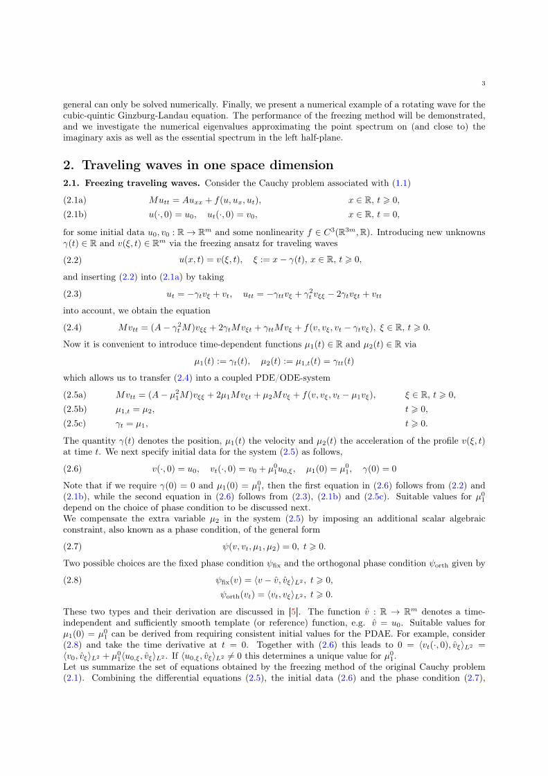
equation (2.10) admits a traveling front solution connecting the asymptotic states v− = 0 and v+ = 1.Figure 2.1 shows a numerical simulation of the solution u of (2.10) on the spatial domain (−50, 50) withhomogeneous Neumann boundary conditions, with initial data

u0(x) = 12

(1 + tanh

(x2

)), v0(x) = 0(2.13)

and parameters taken from (2.12). For the space discretization we use continuous piecewise linear finiteelements with spatial stepsize 4x = 0.1. For the time discretization we use the BDF method of order 2with absolute tolerance atol = 10−3, relative tolerance rtol = 10−2, temporal stepsize 4t = 0.2 and finaltime T = 800. Computations are performed with the help of the software COMSOL 5.2.Let us now consider the frozen quintic Nagumo wave equation resulting from (2.9)

εvtt + vt = (1− µ21ε)vξξ + 2µ1εvξ,t + (µ2ε+ µ1)vξ + f(v),

µ1,t = µ2, γt = µ1,t > 0,(2.14a)

0 =⟨vt(·, t), vξ

⟩L2(R,R)

, t > 0,(2.14b)

v(·, 0) = u0, vt(·, 0) = v0 + µ01u0,ξ, µ1(0) = µ0

1, γ(0) = 0.(2.14c)

5

(a) (b)

Figure 2.1. Traveling front of quintic Nagumo wave equation (2.10) at different timeinstances (a) and its time evolution (b) for parameters from (2.12).

(a) (b) (c)

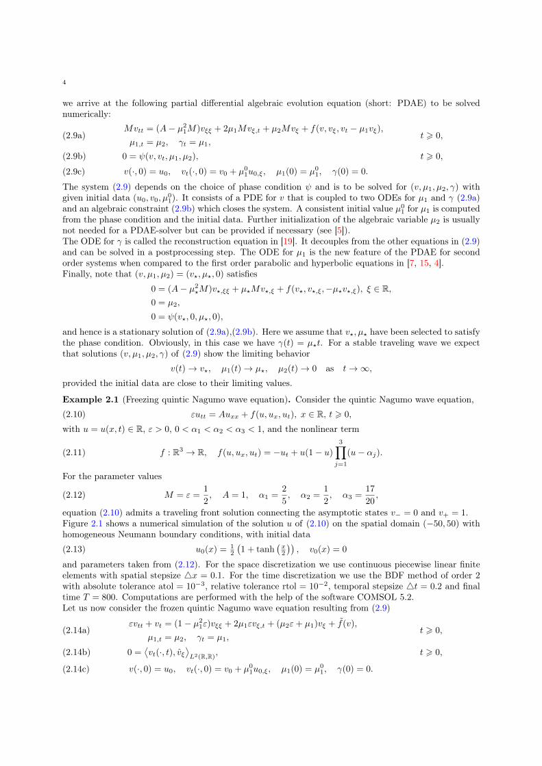
Figure 2.2. Solution of the frozen quintic Nagumo wave equation (2.14): approximationof profile v(x, 1000) (a) and time evolutions of velocity µ1 and acceleration µ2 (b) and ofthe profile v (c) for parameters from (2.12).

Figure 2.2 shows the solution (v, µ1, µ2, γ) of (2.14) on the spatial domain (−50, 50) with homogeneousNeumann boundary conditions, initial data u0, v0 from (2.13), and reference function v = u0. For thecomputation we used the fixed phase condition ψfix(v) from (2.8) with consistent intial data µ0

1 = 0, seeabove. The spatial discretization data are taken as in the nonfrozen case. For the time discretizationwe used the BDF method of order 2 with absolute tolerance atol = 10−3, relative tolerance rtol = 10−2,temporal stepsize 4t = 0.6 and final time T = 3000. The diagrams show that after a very short transitionphase the profile becomes stationary, the acceleration µ2 converges to zero, and the speed µ1 approachesan asymptotic value µnum

? ≈ 0.0709 which is close to the exact (not explicitly known) value µ?.

2.2. Spectra of traveling waves. Consider the linearized equation

(2.15) Mvtt − (A− µ2?M)vξξ − 2µ?Mvξt − (D2f? − µ?D3f?)vξ −D3f?vt −D1f?v = 0

which is obtained from the co-moving frame (1.3) linearized at the profile v?. In (2.15) we use the shortform Djf? = Djf(v?, v?,ξ,−µ?v?,ξ). Looking for solutions of the form v(ξ, t) = eλtw(ξ) to (2.15) yieldsthe quadratic eigenvalue problem

(2.16) P(λ)w =(λ2P2 + λP1 + P0

)w = 0, ξ ∈ R

with differential operators Pj defined by

P2 = M, P1 = −2µ?M∂ξ −D3f?, P0 = −(A− µ2?M)∂2

ξ − (D2f? − µ?D3f?)∂ξ −D1f?.

We are interested in solutions (λ,w) of (2.16) which are candidates for eigenvalues λ ∈ C and eigenfunctionsw : R→ Cm in suitable function spaces. In fact, it is usually imposssible to determine the spectrum σ(P)analytically, but one is able to analyze certain subsets. Let us first calculate the symmetry set σsym(P),

6

which belongs to the point spectrum σpt(P) and is affected by the underlying group symmetries. Then,we calculate the dispersion set σdisp(P), which belongs to the essential spectrum σess(P) and is affectedby the far-field behavior of the wave. Let us first derive the symmetry set of P. This is a simple taskfor traveling waves but becomes more involved when analyzing the symmetry set for rotating waves (seeSection 3.2.1).

2.2.1. Point Spectrum and symmetry set. Applying ∂ξ to the traveling wave equation (1.4) yieldsP0v?,ξ = 0 which proves the following result.

Proposition 2.2 (Point spectrum of traveling waves). Let f ∈ C1(R3m,Rm) and let v? ∈ C3(R,Rm) bea nontrivial classical solution of (1.4) for some µ? ∈ R. Then, w = v?,ξ and λ = 0 is a classical solution ofthe eigenvalue problem (2.16). In particular, the symmetry set

σsym(P) = 0

belongs to the point spectrum σpt(P) of P.

Of course, a rigorous statement of this kind requires to specify the function spaces involved, e.g. L2(R,Rm)or H1(R,Rm), see [10], [9], [5].

2.2.2. Essential Spectrum and dispersion set.1. The far-field operator. It is a well known fact that the essential spectrum is affected by the limiting

equation obtained from (2.16) as ξ → ±∞. Therefore, we let formally ξ → ±∞ in (2.16) and obtain

(2.17)(λ2P2 + λP±1 + P±0

)w = 0, ξ ∈ R.

with the constant coefficient operators

P2 = M, P±1 = −2µ?M∂ξ −D3f±, P±0 = −(A− µ2?M)∂2

ξ − (D2f± − µ?D3f±)∂ξ −D1f±,

where v± are from (1.2) and Djf± = Djf(v±, 0, 0). We may then write equation (2.16) as(λ2P2 + λ(P±1 +Q±1 (ξ)) + (P±0 +Q±2 (ξ)∂ξ +Q±3 (ξ))

)w = 0, ξ ∈ R

with the perturbation operators defined by

Q±1 (ξ) = D3f± −D3f?, Q±2 (ξ) = D2f± −D2f? + µ?(D3f? −D3f±), Q±3 (ξ) = D1f± −D1f?,

Note that v?(ξ)→ v± implies Q±j (ξ)→ 0 as ξ → ±∞ for j = 1, 2, 3.2. Spatial Fourier transform. For ω ∈ R, z ∈ Cm, |z| = 1 we apply the spatial Fourier transform

w(ξ) = eiωξz to equation (2.17) which leads to the m-dimensional quadratic eigenvalue problem

(2.18)(λ2A2 + λA±1 (ω) +A±0 (ω)

)z = 0

with matrices A2 ∈ Rm,m and A±1 , A±0 ∈ Cm,m given by

(2.19) A2 = M, A±1 (ω) = −2iωµ?M −D3f±, A±0 (ω) = ω2(A− µ2

?M)− iω(D2f± − µ?D3f±)−D1f±.

3. Dispersion relation and dispersion set. The dispersion relation for traveling waves of second orderevolution equations states the following: Every λ ∈ C satisfying

(2.20) det(λ2A2 + λA±1 (ω) +A±0 (ω)

)= 0

for some ω ∈ R belongs to the essential spectrum of P, i.e. λ ∈ σess(P). Solving (2.20) is equivalentto finding all zeros of a polynomial of degree 2m. Note that the limiting case M = 0 in (2.20) leadsto the dispersion relation for traveling waves of first order evolution equations, which is well-known inthe literature, see [20].

Proposition 2.3 (Essential spectrum of traveling waves). Let f ∈ C1(R3m,Rm) with f(v±, 0, 0) = 0for some v± ∈ Rm. Let v? ∈ C2(R,Rm), µ? ∈ R be a nontrivial classical solution of (1.4) satisfyingv?(ξ)→ v± as ξ → ±∞. Then, the dispersion set

σdisp(P) = λ ∈ C : λ satisfies (2.20) for some ω ∈ R, and + or −

belongs to the essential spectrum σess(P) of P.

7

Example 2.4 (Spectrum of quintic Nagumo wave equation). As shown in Example 2.1 the quintic Nagumowave equation (2.10) with coefficients and parameters (2.12) has a traveling front solution u?(x, t) =v?(x− µ?t) with velocity µ? ≈ 0.0709, whose profile v? connects the asymptotic states v− = 0 and v+ = 1according to (1.2).We solve numerically the eigenvalue problem for the quintic Nagumo wave equation(

λ2ε+ λ (−2µ?ε∂ξ −D3f?) +(−(1− µ2

?ε)∂2ξ − (D2f? − µ?D3f?)∂ξ −D1f?

))w = 0.(2.21)

Both approximations of the profile v? and the velocity µ? in (2.21) are chosen from the solution of (2.14)at time t = 3000 in Example 2.1. Due to Proposition 2.2 we expect λ = 0 to be an isolated eigenvaluebelonging to the point spectrum. Let us next discuss the dispersion set from Proposition 2.3. The quinticNagumo nonlinearity (2.11) satisfies

f± = 0, D3f± = −1, D2f± = 0, D1f− = −α1α2α3, D1f+ = −3∏j=1

(1− αj).

The matrices A2, A±1 (ω), A±0 (ω) from (2.19) of the quadratic problem (2.18) are given by

A2 = ε, A±1 (ω) = −2iωµ?ε+ 1, A±0 (ω) = ω2(1− µ2?ε)− iωµ? −D1f±.

The dispersion relation (2.20) for the quintic Nagumo front states that every λ ∈ C satisfying

(2.22) λ2ε+ λ(−2iωµ?ε+ 1) + (ω2(1− µ2?ε)− iωµ? −D1f±) = 0

for some ω ∈ R, and for + or −, belongs to σess(P). We introduce a new unknown λ ∈ C via λ = λ+ iωµ?and solve the transformed equation

λ2 +1

ελ+

1

ε(ω2 −D1f±) = 0.

obtained from (2.22). Thus, the quadratic eigenvalue problem (2.22) has the solutions

λ = − 1

2ε+ iωµ? ±

1

2ε

√1− 4ε(ω2 −D1f±), ω ∈ R.

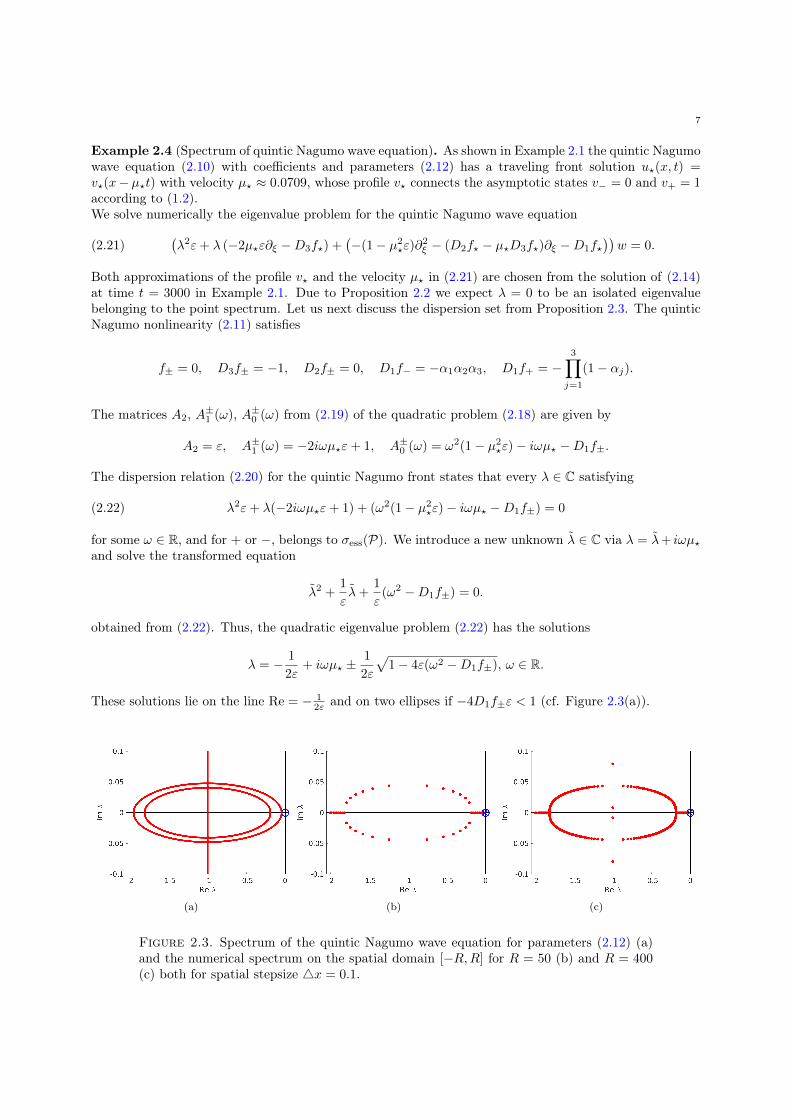
These solutions lie on the line Re = − 12ε and on two ellipses if −4D1f±ε < 1 (cf. Figure 2.3(a)).

(a) (b) (c)

Figure 2.3. Spectrum of the quintic Nagumo wave equation for parameters (2.12) (a)and the numerical spectrum on the spatial domain [−R,R] for R = 50 (b) and R = 400(c) both for spatial stepsize 4x = 0.1.

8

(a) (b) (c)

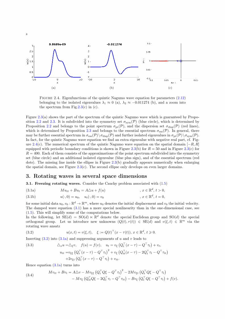
Figure 2.4. Eigenfunctions of the quintic Nagumo wave equation for parameters (2.12)belonging to the isolated eigenvalues λ1 ≈ 0 (a), λ2 ≈ −0.011274 (b), and a zoom intothe spectrum from Fig.2.3(c) in (c).

Figure 2.3(a) shows the part of the spectrum of the quintic Nagumo wave which is guaranteed by Propo-sition 2.2 and 2.3. It is subdivided into the symmetry set σsym(P) (blue circle), which is determined byProposition 2.2 and belongs to the point spectrum σpt(P), and the dispersion set σdisp(P) (red lines),which is determined by Proposition 2.3 and belongs to the essential spectrum σess(P). In general, theremay be further essential spectrum in σess(P)\σdisp(P) and further isolated eigenvalues in σpt(P)\σsym(P).In fact, for the quintic Nagumo wave equation we find an extra eigenvalue with negative real part, cf. Fig-ure 2.4(c). The numerical spectrum of the quintic Nagumo wave equation on the spatial domain [−R,R]equipped with periodic boundary conditions is shown in Figure 2.3(b) for R = 50 and in Figure 2.3(c) forR = 400. Each of them consists of the approximations of the point spectrum subdivided into the symmetryset (blue circle) and an additional isolated eigenvalue (blue plus sign), and of the essential spectrum (reddots). The missing line inside the ellipse in Figure 2.3(b) gradually appears numerically when enlargingthe spatial domain, see Figure 2.3(c). The second ellipse only develops on even larger domains.

3. Rotating waves in several space dimensions3.1. Freezing rotating waves. Consider the Cauchy problem associated with (1.5)

Mutt +But = A4u+ f(u) , x ∈ Rd, t > 0,(3.1a)

u(·, 0) = u0, ut(·, 0) = v0 , x ∈ Rd, t = 0,(3.1b)

for some initial data u0, v0 : Rd → Rm, where u0 denotes the initial displacement and v0 the initial velocity.The damped wave equation (3.1) has a more special nonlinearity than in the one-dimensional case, see(1.5). This will simplify some of the computations below.In the following, let SE(d) = SO(d) n Rd denote the special Euclidean group and SO(d) the specialorthogonal group. Let us introduce new unknowns (Q(t), τ(t)) ∈ SE(d) and v(ξ, t) ∈ Rm via therotating wave ansatz

(3.2) u(x, t) = v(ξ, t), ξ := Q(t)>(x− τ(t)), x ∈ Rd, t > 0.

Inserting (3.2) into (3.1a) and suppressing arguments of u and v leads to

4xu =4ξv, f(u) = f(v), ut = vξ(Q>t (x− τ)−Q>τt

)+ vt,(3.3)

utt =vξξ(Q>t (x− τ)−Q>τt

)2+ vξ

(Q>tt(x− τ)− 2Q>t τt −Q>τtt

)+2vξt

(Q>t (x− τ)−Q>τt

)+ vtt.

Hence equation (3.1a) turns into

(3.4)Mvtt +Bvt = A4v −Mvξξ

(Q>t Qξ −Q>τt

)2 − 2Mvξt(Q>t Qξ −Q>τt

)−Mvξ

(Q>ttQξ − 2Q>t τt −Q>τtt

)−Bvξ

(Q>t Qξ −Q>τt

)+ f(v).

9

It is convenient to introduce time-dependent functions S1(t), S2(t) ∈ Rd,d, µ1(t), µ2(t) ∈ Rd via

S1 := Q>Qt, S2 := S1,t, µ1 := Q>τt, µ2 := µ1,t.

Obviously, S1 and S2 satisfy S>1 = −S1 and S>2 = −S2, which follows from Q>Q = Id by differentiation.Moreover, we obtain

Q>t Q = −S1, Q>τt = µ1, Q>t τt +Q>τtt = µ2,

Q>ttQ = −S1,t − S>1 S1 = −S2 + S21 , −Q>t τt = −Q>t QQ>τt = S1µ1,

which transforms (3.4) into the system

Mvtt +Bvt = A4v −Mvξξ (S1ξ + µ1)2

+ 2Mvξt (S1ξ + µ1)(3.5a)

+Mvξ((S2 − S2

1)ξ − S1µ1 + µ2

)+Bvξ (S1ξ + µ1) + f(v),(

S1

µ1

)t

=

(S2

µ2

),(3.5b) (

Qτ

)t

=

(QS1

Qµ1

).(3.5c)

The quantity (Q(t), τ(t)) describes the position by its spatial shift τ(t) and the rotation Q(t). Moreover,S1(t) denotes the rotational velocities, µ1(t) the translational velocities, S2(t) the angular acceleration andµ2(t) the translational acceleration of the rotating wave v at time t. Note that in contrast to the travelingwaves the leading part A4−M∂2

ξ (S1ξ + µ1)2 not only depends on the velocities S1 and µ1, but also onthe spatial variable ξ, which means that the leading part has unbounded (linearly growing) coefficients.We next specify initial data for the system (3.5) as follows,

(3.6)v(·, 0) = u0, vt(·, 0) = v0 + u0,ξ(S

01ξ + µ0

1),

S1(0) = S01 , µ1(0) = µ0

1, Q(0) = Id, τ(0) = 0.

Note that, requiring Q(0) = Id, τ(0) = 0, S1(0) = S01 and µ1(0) = µ0

1 for some S01 ∈ Rd,d with (S0

1)> = −S01

and µ01 ∈ Rd, the first equation in (3.6) follows from (3.2) and (3.1b), while the second condition in (3.6)

can be deduced from (3.3), (3.1b), (3.5c) and the first condition in (3.6).The system (3.5) comprises evolution equations for the unknowns v, S and µ1. In order to specify theremaining variables S2 and µ2 we impose dim SE(d) = d(d+1)

2 additional scalar algebraic constraints, alsoknown as phase conditions

ψ(v, vt, (S1, µ1), (S2, µ2)) = 0 ∈ Rd(d+1)

2 , t > 0.(3.7)

Two possible choices of such a phase condition are

ψfix(v) :=

(〈v − v, Dlv〉L2

〈v − v, D(i,j)v〉L2

)= 0, t > 0,(3.8)

ψorth(vt) :=

(〈vt, Dlv〉L2

〈vt, D(i,j)v〉L2

)= 0, t > 0,(3.9)

for l = 1, . . . , d, i = 1, . . . , d− 1 and j = i+ 1, . . . , d with Dl := ∂ξl and D(i,j) := ξj∂ξi − ξi∂ξj . Condition(3.8) is obtained from the requirement that the distance

ρ(Q, τ) :=∥∥v(·, t)− v(Q>(· − τ))

∥∥2

L2

attains a local minimum at (Q, τ) = (Id, 0). Since Dl, D(i,j) are the generators of the Euclidean group

action, condition (3.9) requires the time derivative of v to be orthogonal to the group orbit of v at anytime instance.Combining the differential equations (3.5), the initial data (3.6) and the phase condition (3.7), we obtainthe following partial differential algebraic evolution equation (PDAE)

Mvtt +Bvt = A4v −Mvξξ (S1ξ + µ1)2

+ 2Mvξt (S1ξ + µ1)(3.10a)

+Mvξ((S2 − S2

1)ξ − S1µ1 + µ2

)+Bvξ (S1ξ + µ1) + f(v), ξ ∈ Rd, t > 0,

10

v(·, 0) = u0, vt(·, 0) = v0 + u0,ξ(S01ξ + µ0

1), ξ ∈ Rd, t = 0,(3.10b)0 = ψ(v, vt, (S1, µ1), (S2, µ2)), t > 0,(3.10c) (S1

µ1

)t

=

(S2

µ2

),

(S1(0)µ1(0)

)=

(S0

1

µ01

), t > 0,(3.10d) (

Qτ

)t

=

(QS1

Qµ1

),

(Q(0)τ(0)

)=

(Id0

), t > 0.(3.10e)

The system (3.10) depends on the choice of phase condition and must be solved for (v, S1, µ1, S2, µ2, Q, τ)for given (u0, v0, S

01 , µ

01). It consists of a PDE for v in (3.10a)–(3.10b), two systems of ODEs for (S1, µ1) in

(3.10d) and for (Q, τ) in (3.10e) and d(d+1)2 algebraic constraints for (S2, µ2) in (3.10c). The ODE (3.10e)

for (Q, τ) is the reconstruction equation (see [19]), it decouples from the other equations in (3.10) and canbe solved in a postprocessing step. Note that in the frozen equation for first order evolution equations,the ODE for (S1, µ1) does not appear, see [13, (10.26)]. The additional ODE is a new component of thePDAE and is caused by the second order time derivative.Finally, note that (v, S1, µ1, S2, µ2) = (v?, S?, µ?, 0, 0) satisfies

0 = A4v −Mv?,ξξ (S?ξ + µ?)2 −Mv?,ξS? (S?ξ + µ?) +Bv?,ξ (S?ξ + µ?) + f(v?), ξ ∈ Rd,

0 =

(S2

µ2

).

If, in addition, it has been arranged that v?, S?, µ? satisfy the phase condition ψ(v?, 0, S?, µ?, 0, 0) = 0then (v?, S?, µ?, 0, 0) is a stationary solution of the system (3.10a),(3.10c),(3.10d). For a stable rotatingwave we expect that solutions (v, S1, µ1, S2, µ2) of (3.10a)–(3.10d) satisfy

v(t)→ v?, (S1(t), µ1(t))→ (S?, µ?), (S2(t), µ2(t))→ (0, 0), as t→∞,provided the initial data are close to their limiting values.

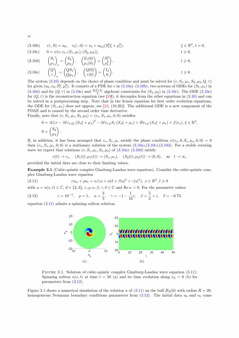
Example 3.1 (Cubic-quintic complex Ginzburg-Landau wave equation). Consider the cubic-quintic com-plex Ginzburg-Landau wave equation

(3.11) εutt + ρut = α4u+ u(δ + β|u|2 + γ|u|4), x ∈ Rd, t > 0

with u = u(x, t) ∈ C, d ∈ 2, 3, ε, ρ, α, β, γ, δ ∈ C and Reα > 0. For the parameter values

ε = 10−4, ρ = 1, α =3

5, γ = −1− 1

10i, β =

5

2+ i, δ = −0.73.(3.12)

equation (3.11) admits a spinning soliton solution.

(a) (b)

Figure 3.1. Solution of cubic-quintic complex Ginzburg-Landau wave equation (3.11):Spinning soliton u(x, t) at time t = 50 (a) and its time evolution along x2 = 0 (b) forparameters from (3.12).

Figure 3.1 shows a numerical simulation of the solution u of (3.11) on the ball BR(0) with radius R = 20,homogeneous Neumann boundary conditions parameters from (3.12). The initial data u0 and v0 come

11

from a simulation. To generate the initial data we consider the case ε = 0 and ρ = 1, solve the frozenQCGL for parameters

α =1

2+

1

2i, γ = −1− 1

10i, β =

5

2+ i, δ = −1

2.

as in [13]. Since this value of α leads to an ill-posed wave equation, we gradually change the value of δand α to arrive at the parameter setting (3.12). For the space discretization we use continuous piecewiselinear finite elements with spatial stepsize 4x = 0.8. For the time discretization we use the BDF methodof order 2 with absolute tolerance atol = 10−4, relative tolerance rtol = 10−3, temporal stepsize 4t = 0.1and final time T = 50. Computations are performed with the help of the software COMSOL 5.2.Let us now consider the frozen cubic-quintic complex Ginzburg-Landau wave equation resulting from (3.10)

εvtt + ρvt = α4v − εvξξ (S1ξ + µ1)2

+ 2εvξt (S1ξ + µ1)(3.13a)

+ εvξ((S2 − S2

1)ξ − S1µ1 + µ2

)+ ρvξ (S1ξ + µ1) + f(v), ξ ∈ Rd, t > 0,

v(·, 0) = u0, vt(·, 0) = v0 + u0,ξ(S01ξ + µ0

1), ξ ∈ Rd, t = 0,(3.13b)

0 = ψfix(v) :=

(〈v − v, Dlv〉L2

〈v − v, D(i,j)v〉L2

), t > 0,(3.13c) (

S1

µ1

)t

=

(S2

µ2

),

(S1(0)µ1(0)

)=

(S0

1

µ01

), t > 0,(3.13d) (

Qτ

)t

=

(QS1

Qµ1

),

(Q(0)τ(0)

)=

(Id0

), t > 0.(3.13e)

(a) (b)

(c) (d)

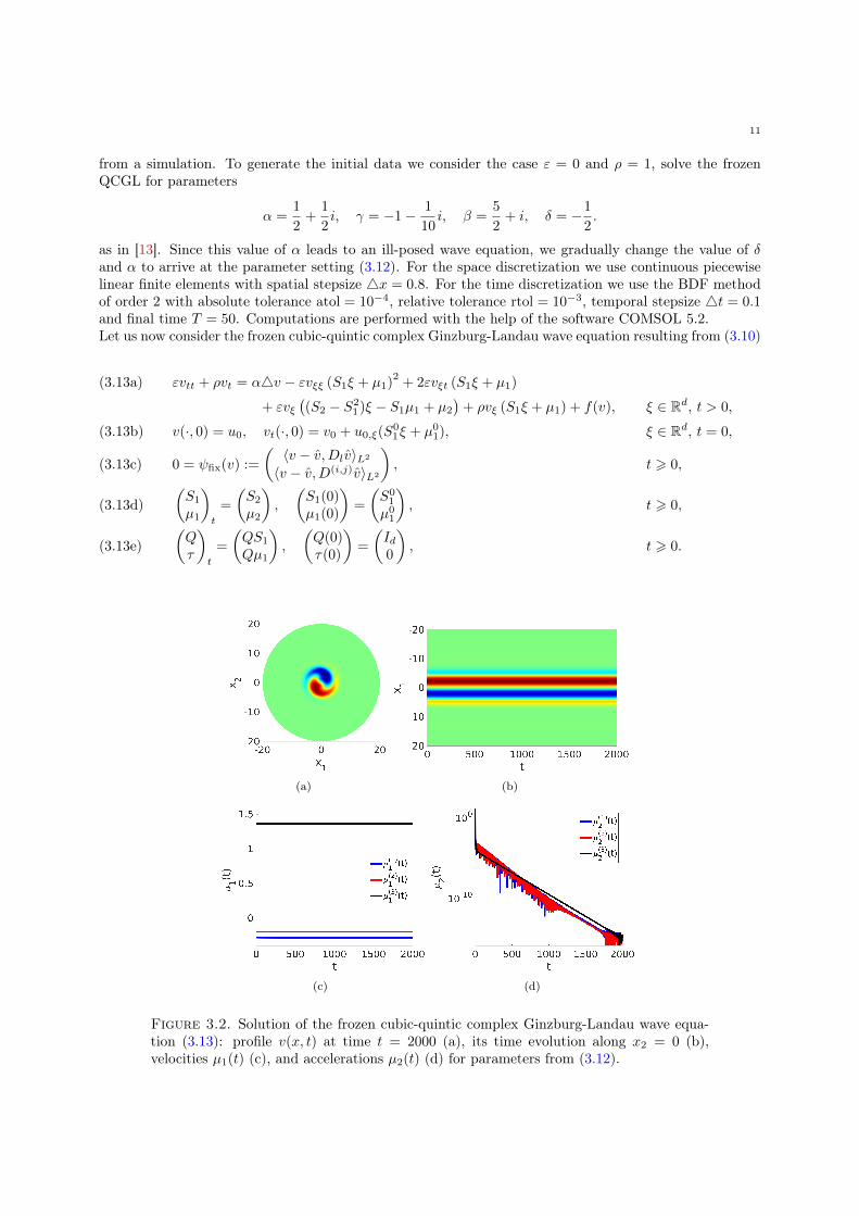
Figure 3.2. Solution of the frozen cubic-quintic complex Ginzburg-Landau wave equa-tion (3.13): profile v(x, t) at time t = 2000 (a), its time evolution along x2 = 0 (b),velocities µ1(t) (c), and accelerations µ2(t) (d) for parameters from (3.12).

12

Figure 3.2 shows the solution (v, S1, µ1, S2, µ2, Q, τ) of (3.13) on the ball BR(0) with radius R = 20,homogeneous Neumann boundary conditions, initial data u0, v0 as in the nonfrozen case, and referencefunction v = u0. For the computation we used the fixed phase condition ψfix(v) from (3.8). The spatialdiscretization data are taken as in the nonfrozen case. For the time discretization we used the BDF methodof order 2 with absolute tolerance atol = 10−3, relative tolerance rtol = 10−2, maximal temporal stepsize4t = 0.5, initial step 10−4, and final time T = 2000. Due to the choice of initial data, the profile becomesimmediately stationary, the acceleration µ2 converges to zero, while the speed µ1 and the nontrivial entryS12 of S approach asymptotic values

µ(1)1 = −0.2819, µ

(2)1 = −0.1999, S12 = 1.3658.

Note that we have a clockwise rotation if S12 > 0, and a counter clockwise rotation, if S12 < 0. Thus,the spinning soliton rotates clockwise. The center of rotation x? and the temporal period T 2D, that thespinning soliton in R2 needs for exactly one rotation, are given by, see [13, Exa.10.8],

x? =1

S12

(µ

(2)1

−µ(1)1

)=

(−0.14640.2064

), T 2D =

2π

|S12|= 4.6004.

3.2. Spectra of rotating waves. Consider the linearized equation

(3.14) Mvtt +Bvt −A4v +Mvξξ(S?ξ)2 − 2MvξtS?ξ +MvξS

2?ξ −BvξS?ξ −Df(v?)v = 0

where we set S = S?. Equation (3.14) is obtained from the co-rotating frame equation (1.6) whenlinearizing at the profile v?. Moreover, we assume µ? = 0, that is the wave that rotates about the origin.Shifting the center of rotation does not influence the stability properties, see the discussion in [3]. Lookingfor solutions of the form v(ξ, t) = eλtw(ξ) to (3.14) yields the quadratic eigenvalue problem

(3.15) P(λ)w :=(λ2P2 + λP1 + P0

)w = 0, ξ ∈ Rd

with differential operators Pj defined by

(3.16)

P2 =M, P1 = B − 2M (∂ξ ·)S?ξ = B − 2M

d∑j=1

(S?ξ)j∂ξj ,

P0 =−A4 ·+M(∂2ξ ·)

(S?ξ)2 +M (∂ξ ·)S2

?ξ −B (∂ξ ·)S?ξ −Df(v?) ·

=−Ad∑j=1

∂2ξj +M

d∑j=1

d∑ν=1

(S?ξ)j(S?ξ)ν∂ξj∂ξν +M

d∑j=1

(S2?ξ)j∂ξj −B

d∑j=1

(S?ξ)j∂ξj −Df(v?).

As in the one-dimensional case we cannot solve equation (3.15) in general. Rather, our aim is to determinethe dispersion set σdisp(P) as a subset of the essential spectrum σess(P), and the symmetry set σsym(P)as a subset of the point spectrum σpt(P). The essential spectrum depends on the far-field behavior of thewave while the point spectrum is affected by the underlying group symmetries.In a first step let us transform the skew-symmetric matrix S? into quasi-diagonal real form. Let±iσ1, . . . ,±iσkbe the nonzero eigenvalues of S? so that 0 is a semisimple eigenvalue of multiplicity d − 2k. There is anorthogonal matrix P ∈ Rd,d such that

S? = PΛP>, Λ = diag (Λ1, . . . ,Λk,0) , Λj =

(0 σj−σj 0

), 0 ∈ Rd−2k,d−2k.

The transformation w(y) = w(Py), v?(y) = v?(Py) transfers (3.15),(3.16) into the form

(3.17) (λ2P2 + λP1 + P0)w = 0.

With the abbreviations

(3.18) Dj = ∂yj , D(i,j) = yjDi − yiDj , K =

k∑l=1

σlD(2l−1,2l)

13

the operators Pj are given by

(3.19)

P2 =M, P1 = B − 2M

d∑j=1

(Λy)jDj = B − 2MK,

P0 =−A4+M

d∑j=1

d∑ν=1

(Λy)j(Λy)νDjDν +M

d∑j=1

(Λ2y)jDj −Bd∑j=1

(Λy)jDj −Df(v?)

=−A4+MK2 −BK −Df(v?).

In the following we present the recipe for computing the subsets σdisp(P) ⊆ σess(P) and σsym(P) ⊆ σpt(P).

3.2.1. Essential spectrum and dispersion set.1. The far-field operator. Assume that v? has an asymptotic state v∞ ∈ Rm, i.e. f(v∞) = 0 and

v?(ξ) → v∞ ∈ Rm as |ξ| → ∞. In the limit |y| → ∞ the eigenvalue problem (3.17) turns into thefar-field problem

(3.20)(λ2P2 + λP1 + P∞

)w = 0, y ∈ Rd, P∞ = −A4+MK2 −BK −Df(v∞).

2. Transformation into several planar polar coordinates: Since we have k angular derivatives in kdifferent planes it is advisable to transform into several planar polar coordinates via(

y2l−1

y2l

)= T (rl, φl) :=

(rl cosφlrl sinφl

), φl ∈ [−π, π), rl ∈ (0,∞), l = 1, . . . , k.

All further coordinates, i.e. y2k+1, . . . , yd, remain fixed. The transformation w(ψ) := w(T2(ψ)) withT2(ψ) = (T (r1, φ1), . . . , T (rk, φk), y2k+1, . . . , yd) for ψ = (r1, φ1, . . . , rk, φk, y2k+1, . . . , yd) in the domainΩ = ((0,∞)× [−π, π))k × Rd−2k transfers (3.20) into

(3.21)(λ2P2 + λP1 + P∞

)w = 0, ψ ∈ Ω

with

P2 = M, P1 = B + 2M

k∑l=1

σl∂φl ,

P∞ = −A[ k∑l=1

(∂2rl

+1

rl∂φl +

1

r2l

∂2φl

)+

d∑l=2k+1

∂2yl

]+M

k∑l,n=1

σlσn∂φl∂φn +B

k∑l=1

σl∂φl −Df(v∞).

3. Simplified far-field operator: The far-field operator (3.21) can be further simplified by lettingrl →∞ for any 1 6 l 6 k which turns (3.21) into

(3.22)(λ2P2 + λP1 + P sim

∞

)w = 0, ψ ∈ Ω

with

(3.23) P sim∞ = −A

[k∑l=1

∂2rl

+

d∑l=2k+1

∂2yl

]+M

k∑l,n=1

σlσn∂φl∂φn +B

k∑l=1

σl∂φl −Df(v∞).

4. Angular Fourier transform: Finally, we solve for eigenvalues and eigenfunctions of (3.23) by sep-aration of variables and an angular resp. radial Fourier ansatz with ω ∈ Rk, ρ, y ∈ Rd−2k, n ∈ Zk,z ∈ Cm, |z| = 1, r ∈ (0,∞)k, φ ∈ (−π, π]k:

w(ψ) = exp

(i

k∑l=1

ωlrl

)exp

(i

k∑l=1

nlφl

)exp

(i

d∑l=2k+1

ρlyl

)z = exp (i〈ω, r〉+ i〈n, φ〉+ i〈ρ, y〉) z.

Inserting this in (3.22) leads to the m-dimensional quadratic eigenvalue problem

(3.24)(λ2A2 + λA1(n) +A∞(ω, n, ρ)

)z = 0

14

with matrices A2 ∈ Rm,m and A1(n), A∞(ω, n, ρ) ∈ Cm,m given by

(3.25)A2 =M, A1(n) = B + 2i〈σ, n〉M,

A∞(ω, n, ρ) =(|ω|2 + |ρ|2

)A− 〈σ, n〉2M + i〈σ, n〉B −Df(v∞).

The Fourier ansatz is a well-known tool for investigating essential spectra, see e.g. [8].5. Dispersion relation and dispersion set: As in Section 2.2.2 we consider the dispersion set consisting

of all values λ ∈ C satisfying the dispersion relation

(3.26) det(λ2A2 + λA1(n) +A∞(ω, n, ρ)

)= 0

for some ω ∈ Rk, ρ ∈ Rd−2k and n ∈ Zk. Of course, one can replace |ω|2 + |ρ|2 by any nonnegative realnumber. Solving (3.26) is equivalent to finding all zeros of a parameterized polynomial of degree 2m.Note that the limiting case M = 0 and B = Im in (3.26) leads to the dispersion relation for rotatingwaves of first order evolution equations, see [1] for d = 2, and [13, Sec. 7.4 and 9.4], [2] for generald > 2.

Using standard cut-off arguments as in [1],[13],[2], the following result can be shown for suitable functionspaces (e.g. L2(Rd,Rm)):

Proposition 3.2 (Essential spectrum of rotating waves). Let f ∈ C1(Rm,Rm) with f(v∞) = 0 for somev∞ ∈ Rm. Let v? ∈ C2(Rd,Rm) with skew-symmetric S? ∈ Rm,m be a classical solution of (1.7) satisfyingv?(ξ)→ v∞ as |ξ| → ∞. Then, the dispersion set

σdisp(P) = λ ∈ C | λ satisfies (3.26) for some ω ∈ Rk, ρ ∈ Rd−2k, n ∈ Zk

belongs to the essential spectrum σess(P) of the operator polynomial P from (3.15).

3.2.2. Point Spectrum and symmetry set. Recall the SE(d)-group action

[a(R, τ)u](x) = u(R−1(x− τ)), x ∈ Rd, (R, τ) ∈ SE(d).

whose generators are Dl, l = 1, . . . , d and D(a,b), a = 1, . . . , d − 1, b = a + 1, . . . , d from (3.18). Aswith the eigenvalue problem (3.15) we transform the steady state equation (1.7) into y-coordinates viav?(y) = v?(Py) to obtain

(3.27) 0 = Lv? + f(v?), L = A4−MK2 +BK.

We apply the generators (3.18) to this equation and find

(3.28)0 =DlLv? +Df(v?)Dlv?, l = 1, . . . , d,

0 =D(a,b)Lv? +Df(v?)D(a,b)v?, a = 1, . . . , d− 1, b = a+ 1, . . . , d.

Moreover, we can write the eigenvalue problem (3.17), (3.19) as follows

(3.29) (L+Df(v?))w = (λ2M + λ(B − 2MK))w.

1. Linear combination of generators: In view of (3.28),(3.29) it is natural to seek eigenfunctions asa linear combination of generators applied to the profile

(3.30) w =

d−1∑a=1

d∑b=a+1

αrotab D

(a,b)v? +

d∑c=1

αtrac Dcv?, αrot

ab , αtrac ∈ C

This is to be plugged into (3.29) and reduced to an eigenvalue problem for αrot, αtra by using the equations(3.28).2. Commutator relations and eigenvalues of S?: From (3.18) it is straightforward to establish thecommutator relations

(3.31)DcDj = DjDc, DcD

(i,j) = D(i,j)Dc + δcjDi − δciDj

D(a,b)D(i,j) = D(i,j)D(a,b) + δajD(i,b) + δaiD

(b,j) + δbiD(j,a) + δbjD

(a,i).

15

From this we find the commutators with K and 4 to be

(3.32)DcK = KDc (c = 2k + 1, . . . , d), D(2ν−1,2ν)4 = 4D(2ν−1,2ν), D(2ν−1,2ν)K = KD(2ν−1,2ν),

D2ν−1K = KD2ν−1 − σνD2ν , D2νK = KD2ν + σνD2ν−1 (ν = 1, . . . , k).

First, all operators Dc, c = 2k+1, . . . , d commute with L. Hence, by (3.28) the operator L+Df(v?) has theeigenvalue 0 with geometric multiplicity at least d−2k with eigenfunctions given by Dcv?, c = 2k+1, . . . d.Furthermore, we obtain from (3.32) for ν = 1, . . . , k

(3.33)

D2ν−1K2 = K2D2ν−1 − 2σνKD2ν − σ2

νD2ν−1, D2νK2 = K2D2ν + 2σνKD2ν−1 − σ2

νD2ν ,

D2ν−1L = LD2ν−1 − σν(B − 2MK)D2ν + σ2νMD2ν−1,

D2νL =LD2ν + σν(B − 2MK)D2ν−1 + σ2νMD2ν .

Combining the last two rows with (3.28) finally yields

(3.34) (L+Df(v?))(D2ν + iD2ν−1)v? =[(iσν)(B − 2MK) + (iσν)2M

](iD2ν−1 +D2ν)v?,

and similarly for the complex conjugate. Therefore, the quadratic problem (3.29) has eigenvalues ±iσνwith eigenfunctions ±iD2ν−1v? +D2ν v?, ν = 1, . . . k.3. Commutator relations and sums of eigenvalues of S?: Now we use the relation (3.28) for indicesa = 2µ − 1, 2µ and b = 2ν − 1, 2ν with 1 ≤ µ < ν ≤ k. The following commutator relations follow from(3.31)

(3.35) D[µ,ν]K = (KI4 + Σ)D[µ,ν], D[µ,ν] =

D(2µ−1,2ν−1)

D(2µ−1,2ν)

D(2µ,2ν−1)

D(2µ,2ν)

, Σ =

0 −σν −σµ 0σν 0 0 −σµσµ 0 0 −σν0 σµ σν 0

.

Note that Σ is skew-symmetric with eigenvalues ±i(σν ± σµ). We look for eigenfunctions of the specialform

(3.36) w = Lαv?, Lα =∑

a=2µ−1,2µ

∑b=2ν−1,2ν

αa,bD(a,b) = α>D[µ,ν].

Let λ ∈ C be an eigenvalue of Σ with eigenvector α ∈ C4, so that α>Σ = −λα> by skew-symmetry. Thenwe obtain from (3.35)

(3.37) LαK = α>D[µ,ν]K = α>(KI4 + Σ)D[µ,ν] = (K − λ)Lα, LαK2 = (K2 − 2λK + λ2)Lα.

Using (3.27), (3.32) and the fact that scalar differential operators commute with matrices, yields

LαL =Lα(4A−K2M +KB) = 4LαA− (K2 − 2λK + λ2)LαM + (K − λ)LαB

=LLα − (λ2M + λ(B − 2MK))Lα.

Finally, we note that LαLv? = −Df(v?)Lαv? follows from (3.28), which then gives

(L+Df(v?))Lαv? = (LLα − LαL)v? = (λ2M + λ(B − 2MK))Lαv?.

Hence w = Lαv? solves the quadratic eigenvalue problem (3.29). All 4 eigenfunctions can now be read offfrom the columns of the unitary matrix

V =1

4

1 1 1 1−i −i i i−i i −i i−1 1 1 −1

, ΣV = V diag(i(σν + σµ), i(σν − σµ), i(σµ − σν),−i(σν + σµ)).

The computations for the remaining eigenfunctions are similar. Take µ = 1, . . . , k, c = 2k + 1, . . . , d andreplace (3.35) by the relation

D[µ,c]K = (KI4 + Σ)D[µ,c], D[µ,ν] =

D(2µ−1,2µ)

D(2µ−1,c)

D(2µ,c)

, Σ =

0 0 00 0 −σµ0 σµ 0

.

16

For the zero row and column in Σ compare (3.32). Then by the same computations as above one finds thateigenvalues λ of Σ are also eigenvalues of (3.29). The corresponding eigenfunctions are w = α>D[µ,c]〉v?where Σα = λα. Therefore, we have further eigenfunctions D(2µ−1,2µ)v? for the eigenvalue 0 andD(2µ−1,c)v? ± iD(2µ,c)v? for the eigenvalue ±iσµ, µ = 1, . . . , k. Finally, note that for any two indices2k < b < c ≤ d the operator D(b,c) commutes with K and 4, and thus produces another eigenfunctionw = D(b,c)v? which belongs to the eigenvalue 0.Collecting all computations we have found a total of d+4k(k−1)

2 +2k(d−2k)+k+ (d−2k)(d−2k−1)2 = 1

2d(d+1)eigenfunctions corresponding to eigenvalues of S? and to sums of different eigenvalues of S?. In a genericsense we expect these eigenfunctions to be linearly independent, but, of course, one cannot prove this ingeneral. Let us summarize the result in a proposition.

Proposition 3.3 (Point spectrum of rotating waves). Let f ∈ C2(Rm,Rm) and let v? ∈ C3(Rd,Rm) be aclassical solution of (1.7) with skew-symmetric S? ∈ Rm,m. Further, let λj , j = 1, . . . , d be the eigenvaluesof S? repeated according to their multiplicity. Then the symmetry set

σsym(P) = λ ∈ C : λ = λj or λ = λi + λj for some 1 ≤ i < j ≤ d

belongs to the point spectrum σpt(P) of the quadratic operator polynomial P(λ) in (3.15), (3.16) obtainedby linearizing at the wave. The eigenvalues and eigenfunctions of the transformed problem (3.17) aredisplayed in the following table (setting r = d− 2k):

eigenvalue eigenfunction index number0 Dcv? 2k < c ≤ d r±iσν (D2ν ± iD2ν−1)v? 1 ≤ ν ≤ k 2k

±i(σν + σµ) (D(2µ−1,2ν−1) ∓ iD(2µ−1,2ν) ∓ iD(2µ,2ν−1) −D(2µ,2ν))v? 1 ≤ µ < ν ≤ k k(k − 1)

±i(σν − σµ) (D(2µ−1,2ν−1) ± iD(2µ−1,2ν) ∓ iD(2µ,2ν−1) +D(2µ,2ν))v? 1 ≤ µ < ν ≤ k k(k − 1)

±iσν (D(2ν−1,c) ± iD(2ν,c))v? 1 ≤ ν ≤ k, 2k < c ≤ d 2kr

0 D(2ν−1,ν)v? 1 ≤ ν ≤ k k

0 D(b,c)v? 2k < b < c ≤ d r2 (r − 1)

Table 1: Eigenfunctions and eigenvalues (with multiplicities) on the imaginary axis for the linearizedquadratic eigenvalue problem (3.17).

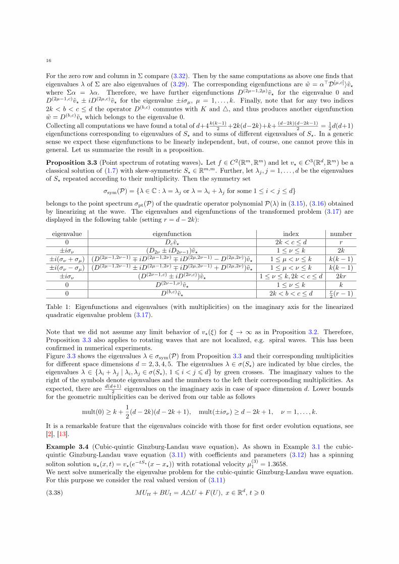
Note that we did not assume any limit behavior of v?(ξ) for ξ → ∞ as in Proposition 3.2. Therefore,Proposition 3.3 also applies to rotating waves that are not localized, e.g. spiral waves. This has beenconfirmed in numerical experiments.Figure 3.3 shows the eigenvalues λ ∈ σsym(P) from Proposition 3.3 and their corresponding multiplicitiesfor different space dimensions d = 2, 3, 4, 5. The eigenvalues λ ∈ σ(S?) are indicated by blue circles, theeigenvalues λ ∈ λi + λj | λi, λj ∈ σ(S?), 1 6 i < j 6 d by green crosses. The imaginary values to theright of the symbols denote eigenvalues and the numbers to the left their corresponding multiplicities. Asexpected, there are d(d+1)

2 eigenvalues on the imaginary axis in case of space dimension d. Lower boundsfor the geometric multiplicities can be derived from our table as follows

mult(0) ≥ k +1

2(d− 2k)(d− 2k + 1), mult(±iσν) ≥ d− 2k + 1, ν = 1, . . . , k.

It is a remarkable feature that the eigenvalues coincide with those for first order evolution equations, see[2], [13].

Example 3.4 (Cubic-quintic Ginzburg-Landau wave equation). As shown in Example 3.1 the cubic-quintic Ginzburg-Landau wave equation (3.11) with coefficients and parameters (3.12) has a spinningsoliton solution u?(x, t) = v?(e

−tS?(x− x?)) with rotational velocity µ(3)1 = 1.3658.

We next solve numerically the eigenvalue problem for the cubic-quintic Ginzburg-Landau wave equation.For this purpose we consider the real valued version of (3.11)

(3.38) MUtt +BUt = A4U + F (U), x ∈ Rd, t > 0

17

Imλ

Reλ

iσ11

01

−iσ11

(a) d = 2

dimSE(2) = 3

Imλ

Reλ

iσ12

02

−iσ12

(b) d = 3

dimSE(3) = 6

Imλ

Reλ

i(σ1 + σ2)1

iσ11

i(σ1 − σ2)1

iσ21

02

−iσ21

−i(σ1 − σ2)1

−iσ11

−i(σ1 + σ2)1

(c) d = 4

dimSE(4) = 10

Imλ

Reλ

i(σ1 + σ2)1

iσ12

i(σ1 − σ2)1

iσ22

03

−iσ22

−i(σ1 − σ2)1

−iσ12

−i(σ1 + σ2)1

(d) d = 5

dimSE(5) = 15

Figure 3.3. Point spectrum of the linearization P on the imaginary axis iR for spacedimension d = 2, 3, 4, 5 given by Proposition 3.3.

with

M =

(ε1 −ε2

ε2 ε1

), B =

(ρ1 −ρ2

ρ2 ρ1

), A =

(α1 −α2

α2 α1

), U =

(u1

u2

),

F (U) =

((U1δ1 − U2δ2) + (U1β1 − U2β2)(U2

1 + U22 ) + (U1γ1 − U2γ2)(U2

1 + U22 )2

(U1δ2 + U2δ1) + (U1β2 + U2β1)(U21 + U2

2 ) + (U1γ2 + U2γ1)(U21 + U2

2 )2

),

(3.39)

where u = u1 + iu2, ε = ε1 + iε2, ρ = ρ1 + iρ2, α = α1 + iα2, β = β1 + iβ2, γ = γ1 + iγ2, δ = δ1 + iδ2 andεj , ρj , αj , βj , γj , δj ∈ R.Now, the eigenvalue problem for the cubic-quintic Ginzburg-Landau wave equation is, cf. (3.15), (3.16),

(λ2M ·+λ [B · −2M(∂ξ·)Sξ] +

[−A4 ·+M(∂2

ξ ·)(Sξ)2 +M(∂ξ·)S2ξ −B(∂ξ·)Sξ −DF (v?)·])w = 0.

(3.40)

Both approximations of the profile v? and the velocity matrix S = S? in (3.40) are chosen from thesolution of (3.13) at time t = 2000 in Example 3.1. By Proposition 3.3 the problem (3.40) has eigenvaluesλ = 0,±iσ. These eigenvalues will be isolated and hence belong to the point spectrum, if the differentialoperator is Fredholm of index 0 in suitable function spaces. For the parabolic case (M = 0) this has beenestablished in [2] and we expect it to hold in the general case as well. Let us next discuss the dispersion setfrom Proposition 3.2. The cubic-quintic Ginzburg-Landau nonlinearity F : R2 → R2 from (3.39) satisfies

(3.41) DF (v∞) =

(δ1 −δ2δ2 δ1

)for v∞ =

(00

).

The matrices A2, A1(n), A∞(ω, n) from (3.25) of the quadratic problem (3.24) are given by

A2 = M, A1(n) = B + 2iσnM, A∞(ω, n) = ω2A− σ2n2M + iσnB −DF (v∞)

for M,B,A from (3.39), DF (v∞) from (3.41), ω ∈ R, n ∈ Z and σ = µ(3)1 . The dispersion relation (3.26)

for the spinning solitons of the Ginzburg-Landau wave equation in R2 states that every λ ∈ C satisfying

det(λ2M + λ(B + 2iσnM) + (ω2A− σ2n2M + iσnB −DF (v∞))

)= 0

for some ω ∈ R and n ∈ Z, belongs to the essential spectrum σess(P) of P. We may rewrite this in complexnotation and find the dispersion set

σdisp(P) = λ ∈ C : λ2ε+ λ(ρ+ 2iσnε) + (ω2α− σ2n2ε+ iσnρ− δ) = 0 for some ω ∈ R, n ∈ Z(3.42)

18

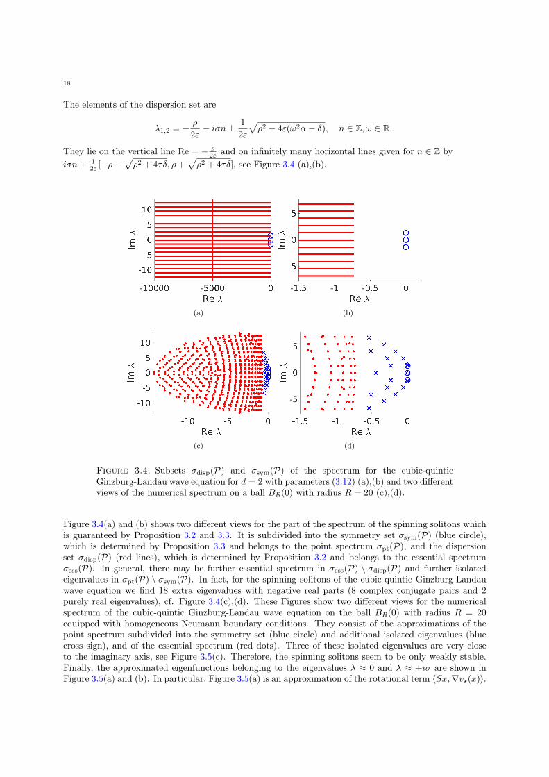
The elements of the dispersion set are

λ1,2 = − ρ

2ε− iσn± 1

2ε

√ρ2 − 4ε(ω2α− δ), n ∈ Z, ω ∈ R..

They lie on the vertical line Re = − ρ2ε and on infinitely many horizontal lines given for n ∈ Z by

iσn+ 12ε [−ρ−

√ρ2 + 4τδ, ρ+

√ρ2 + 4τδ], see Figure 3.4 (a),(b).

(a) (b)

(c) (d)

Figure 3.4. Subsets σdisp(P) and σsym(P) of the spectrum for the cubic-quinticGinzburg-Landau wave equation for d = 2 with parameters (3.12) (a),(b) and two differentviews of the numerical spectrum on a ball BR(0) with radius R = 20 (c),(d).

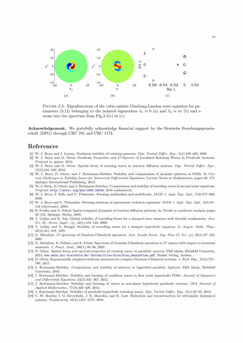
Figure 3.4(a) and (b) shows two different views for the part of the spectrum of the spinning solitons whichis guaranteed by Proposition 3.2 and 3.3. It is subdivided into the symmetry set σsym(P) (blue circle),which is determined by Proposition 3.3 and belongs to the point spectrum σpt(P), and the dispersionset σdisp(P) (red lines), which is determined by Proposition 3.2 and belongs to the essential spectrumσess(P). In general, there may be further essential spectrum in σess(P) \ σdisp(P) and further isolatedeigenvalues in σpt(P) \ σsym(P). In fact, for the spinning solitons of the cubic-quintic Ginzburg-Landauwave equation we find 18 extra eigenvalues with negative real parts (8 complex conjugate pairs and 2purely real eigenvalues), cf. Figure 3.4(c),(d). These Figures show two different views for the numericalspectrum of the cubic-quintic Ginzburg-Landau wave equation on the ball BR(0) with radius R = 20equipped with homogeneous Neumann boundary conditions. They consist of the approximations of thepoint spectrum subdivided into the symmetry set (blue circle) and additional isolated eigenvalues (bluecross sign), and of the essential spectrum (red dots). Three of these isolated eigenvalues are very closeto the imaginary axis, see Figure 3.5(c). Therefore, the spinning solitons seem to be only weakly stable.Finally, the approximated eigenfunctions belonging to the eigenvalues λ ≈ 0 and λ ≈ +iσ are shown inFigure 3.5(a) and (b). In particular, Figure 3.5(a) is an approximation of the rotational term 〈Sx,∇v?(x)〉.

19

(a) (b) (c)

Figure 3.5. Eigenfunctions of the cubic-quintic Ginzburg-Landau wave equation for pa-rameters (3.12) belonging to the isolated eigenvalues λ1 ≈ 0 (a) and λ2 ≈ iσ (b) and azoom into the spectrum from Fig.3.4(c) in (c).

Acknowledgement. We gratefully acknowledge financial support by the Deutsche Forschungsgemein-schaft (DFG) through CRC 701 and CRC 1173.

References[1] W.-J. Beyn and J. Lorenz. Nonlinear stability of rotating patterns. Dyn. Partial Differ. Equ., 5(4):349–400, 2008.[2] W.-J. Beyn and D. Otten. Fredholm Properties and Lp-Spectra of Localized Rotating Waves in Parabolic Systems.

Preprint to appear, 2016.[3] W.-J. Beyn and D. Otten. Spatial decay of rotating waves in reaction diffusion systems. Dyn. Partial Differ. Equ.,

13(3):191–240, 2016.[4] W.-J. Beyn, D. Otten, and J. Rottmann-Matthes. Stability and computation of dynamic patterns in PDEs. In Cur-

rent Challenges in Stability Issues for Numerical Differential Equations, Lecture Notes in Mathematics, pages 89–172.Springer International Publishing, 2014.

[5] W.-J. Beyn, D. Otten, and J. Rottmann-Matthes. Computation and stability of traveling waves in second order equations.Preprint, http://arxiv.org/abs/1606.08844, 2016 (submitted).

[6] W.-J. Beyn, S. Selle, and V. Thümmler. Freezing multipulses and multifronts. SIAM J. Appl. Dyn. Syst., 7(2):577–608,2008.

[7] W.-J. Beyn and V. Thümmler. Freezing solutions of equivariant evolution equations. SIAM J. Appl. Dyn. Syst., 3(2):85–116 (electronic), 2004.

[8] B. Fiedler and A. Scheel. Spatio-temporal dynamics of reaction-diffusion patterns. In Trends in nonlinear analysis, pages23–152. Springer, Berlin, 2003.

[9] T. Gallay and R. Joly. Global stability of travelling fronts for a damped wave equation with bistable nonlinearity. Ann.Sci. Éc. Norm. Supér. (4), 42(1):103–140, 2009.

[10] T. Gallay and G. Raugel. Stability of travelling waves for a damped hyperbolic equation. Z. Angew. Math. Phys.,48(3):451–479, 1997.

[11] G. Metafune. Lp-spectrum of Ornstein-Uhlenbeck operators. Ann. Scuola Norm. Sup. Pisa Cl. Sci. (4), 30(1):97–124,2001.

[12] G. Metafune, D. Pallara, and E. Priola. Spectrum of Ornstein-Uhlenbeck operators in Lp spaces with respect to invariantmeasures. J. Funct. Anal., 196(1):40–60, 2002.

[13] D. Otten. Spatial decay and spectral properties of rotating waves in parabolic systems. PhD thesis, Bielefeld University,2014, www.math.uni-bielefeld.de/~dotten/files/diss/Diss_DennyOtten.pdf. Shaker Verlag, Aachen.

[14] D. Otten. Exponentially weighted resolvent estimates for complex Ornstein-Uhlenbeck systems. J. Evol. Equ., 15(4):753–799, 2015.

[15] J. Rottmann-Matthes. Computation and stability of patterns in hyperbolic-parabolic Systems. PhD thesis, BielefeldUniversity, 2010.

[16] J. Rottmann-Matthes. Stability and freezing of nonlinear waves in first order hyperbolic PDEs. Journal of Dynamicsand Differential Equations, 24(2):341–367, 2012.

[17] J. Rottmann-Matthes. Stability and freezing of waves in non-linear hyperbolic–parabolic systems. IMA Journal ofApplied Mathematics, 77(3):420–429, 2012.

[18] J. Rottmann-Matthes. Stability of parabolic-hyperbolic traveling waves. Dyn. Partial Differ. Equ., 9(1):29–62, 2012.[19] C. W. Rowley, I. G. Kevrekidis, J. E. Marsden, and K. Lust. Reduction and reconstruction for self-similar dynamical

systems. Nonlinearity, 16(4):1257–1275, 2003.

20

[20] B. Sandstede. Stability of travelling waves. In Handbook of dynamical systems, Vol. 2, pages 983–1055. North-Holland,Amsterdam, 2002.

[21] V. Thümmler. Numerical bifurcation analysis of relative equilibria with Femlab. in Proceedings of the COMSOL UsersConference (Comsol Anwenderkonferenz), Frankfurt, Femlab GmbH, Goettingen, Germany, 2006.

[22] V. Thümmler. The effect of freezing and discretization to the asymptotic stability of relative equilibria. J. Dynam.Differential Equations, 20(2):425–477, 2008.

[23] V. Thümmler. Numerical approximation of relative equilibria for equivariant PDEs. SIAM J. Numer. Anal., 46(6):2978–3005, 2008.