Embed Size (px)
Citation preview
Geophysical I’rospectirg, 1997, 4.5, 14 1- 164
Fracture characterization from near-offset VSPinversion’
Steve Horne,2T3 Colin MacBeth,2 J.Queen,4 W.Rizer4 and V. Cox4
Abstract
A global optimization method incorporating a ray-tracing scheme is used to invertobservations of shear-wave splitting from two near-offset VSPs recorded at theConoco Borehole Test Facility, Kay County, Oklahoma. Inversion results suggestthat the seismic anisotropy is due to a non-vertical fracture system. Thisinterpretation is constrained by the VSP acquisition geometry for which two sourcesare employed along near diametrically opposite azimuths about the well heads. Acorrelation is noted between the time-delay variations between the fast and slow splitshear waves and the sandstone formations.
Introduction
Wave propagation in anisotropic media is considerably more complicated than forthe isotropic case. Perhaps the most fundamental complication arises from theexistence of three distinct body waves propagating with different velocities andpolarizations. These form an orthogonally polarized set which is not generallycoincident with the dynamic axes and, except for symmetry directions, cannot bedescribed in terms of P, SH and SV wavetypes. These three body waves are generallyreferred to as the qP (quasi-compressional), qS1 and qS2 (fast and slow quasi-shearwaves) modes. The existence of these two quasi-shear waves travelling with distinctpolarizations and velocities is often referred to as shear-wave birefringence or shear-wave splitting. This phenomenon has been extensively investigated and is ofparticular interest to petroleum geoscientists since shear-wave splitting may beinterpreted in terms of aligned fracture systems (e.g. Crampin and Love11 1991;Mueller 1992). Such information may be critically important to the successfuldevelopment of hydrocarbon reservoirs whose permeability is controlled byfracturing (Ehlig-Economides, Ebbs and Meehan 1990; Ata and Michelena 1995).A method is therefore desirable which may be applied to invert these measurements
’ Received October 1995, revision accepted January 1996.2 British Geological Survey, Murchison House, West Mains Road, Edinburgh, EH9 3LA, Scotland, UK.3 Department of Geology and Geophysics, Grant Institute, University of Edinburgh, West Mains Road,
Edinburgh, EH9 3JW, Scotland, UK.4 Conoco Inc., Ponca City, OK 74603, USA.
0 1997 European Association of Geoscientists & Engineers 141
142 S. Home et al.
of shear-wave splitting. Unfortunately, the formulation of the inverse problemis impeded by the complicated nature of wave propagation in anisotropic media(Helbig 1994). We show how a global optimization method may be applied to thisproblem.
Genetic algorithms
Genetic algorithms (GA) are a class of search methods based on an analogy withnatural evolution (Goldberg 1989). A GA uses a collection of models, analogous to apopulation, which are individually represented in a coded form, analogous to achromosome. These are then manipulated by ‘genetic operators’ in such a way thatbetter models, on average, are generated. Unfortunately, the underlying searchmechanisms explaining the successful behaviour of GAS have yet to be clearlyidentified (Fogel and Stayton 1994). None the less, these methods have generallybeen found to be useful in many diverse fields (Davis 1991), including the geophysicsindustry (e.g. Sen and Stoffa 1992).
Global optimization schemes, such as GAS or simulated annealing, typicallysample several thousands of models during a search so that any forward-modellingscheme requiring more than a few seconds becomes prohibitively expensive incomputational time. We therefore require a forward-modelling scheme which is bothaccurate and efficient. The most suitable approach is offered by a ray-tracing scheme.
Inversion requirements
The ray-tracing method is a high-frequency approximation which effectively followsthe advance of a plane wavefront through a structure by application of Snell’s law.This statement is true for wave propagation in both isotropic and anisotropic mediaalthough Snell’s law needs some reformulation for the anisotropic case (Helbig1994). Ray tracing in continuous anisotropic media essentially requires theintegration of six coupled differential equations (cerveny 1972). These may besolved in a variety of ways for example, using Runge-Kutta methods (Li, Leary andAli 1990) or finite-difference methods (Pereya, Lee and Keller 1980). Although ray-tracing schemes are fast, efficient, and may be applied to complex heterogeneous 3Dstructures, considerable errors may be introduced for singular regions (Gajewski andl?Sen&k 1990). It should also be remembered that ray tracing implicitly assumes planewavefronts so that the calculations are for the phase rather than the group velocities.
The ray-tracing method is a very general technique which may be applied tocomplicated 3D heterogeneous anisotropic models. There will clearly be a trade-offbetween the computational speed and the model complexity. It is therefore possibleto decrease the computational time significantly by increasing the model simplicity.For this reason we approximate the models to a 1D stack of plane layers. A furtherincrease in speed can be achieved if out-of-sagittal-plane deviations are neglected.This reduces the ray-tracing method to a root-searching problem as a function of one
‘: 1’F’7 litlroPcan Association of Geoscientists & Engineers, Geophysical f+o+&ng, 45, 141-164
Fracture characterization 143
variable. This second approximation will be valid in the case of weak anisotropy or in
the case that the propagation plane is a plane of symmetry.
Modelling procedure
The concept that underlies ray tracing in both isotropic and anisotropic media is theconservation of the tangential components of slowness as described by Snell’s law. Inthe case of a horizontally plane layered model, this implies that the horizontalcomponents, p, and pY, are the quantities conserved at the interfaces. In the isotropiccase the vertical component of slowness is simply given by pz = (l/v&, - pz - pz).However, for the anisotropic case, the velocity is a function of the propagationdirection which complicates matters considerably. In the case of triclinic symmetry,the vertical component of slowness, p,, can be derived by the solution of a sexticequation. The use of this equation is to be avoided because of the numericalimprecision associated with round-off errors and the complexity of the coefficients(Fryer and Frazer 1987). However, a considerable simplification is achieved if themedium possesses a monoclinic or a higher symmetry with a horizontal plane ofsymmetry. In this case the slowness may be written in terms of a cubic, the threeroots of which are simply the squares of the vertical slowness, p,.
The approach that we use is initially to construct a table of slowness curves beforeimplementing the ray-tracing algorithm. Intermediate values of slowness can bederived by the application of interpolation methods. This approach has theadvantage that a horizontal plane of symmetry need not be assumed, as is the casewith the analytical slowness equations, but it should be noted that a loss of precisionmay be involved with the interpolation approach. Horizontal and vertical slownessesare calculated for a range of angles of incidence between vertical and horizontaldirections in the sagittal plane by solution of the Kelvin-Christoffel equation. Caremust be taken in the choice of angles of incidence used in the interpolation scheme,since the derivatives of the slowness curve will be sensitive to the horizontal slownesssampling interval. For example, if the slowness curve is sampled with equispacedangles then the errors in the derivatives will increase towards the horizontalpropagation directions. A more appropriate scheme is to calculate the incrementalchange in the angle of incidence so that the horizontal slowness is sampled atapproximately equal intervals.
These interpolation tables are used in the ray-tracing algorithm to calculate thevertical slowness component of a transmitted wave for a given horizontal slowness.The horizontal and vertical slownesses define the propagation direction within thelayer. In this way, the ray may be traced through the stack of layers for a trialhorizontal slowness value. The ray is terminated after it has travelled a horizontaldistance corresponding to the source-geophone distance. The ray-tracing algorithmtherefore searches over the horizontal slowness parameter for a ray connecting thesource and geophone. This is achieved using a shooting method, whereby an initialcourse scan is performed over the horizontal slowness to bracket the solution. The
0 1997 European Association of Geoscientists & Engineers, Geophysical Prospecting, 45, 141-164

144 S. Horne et al.
horizontal slowness root is then refined using standard numerical procedures (Presset al. 1992).
Care must be taken when applying Snell’s law at each interface to ensure that thereis continuity between the incident and transmitted shear waves. This implies that thebody waves must be separated according to the polarization of the wavetype. Forhexagonal materials this may be achieved as one of the shear waves is entirelyindependent of the two other wavetypes (Musgrave 1970) so that it is possible todistinguish the two shear waves by application of the equation
pv$ - c44(1 - 42) - %642 = 0, (1)where the symmetry axis is aligned along the xl-direction, p is the density, Vqs is thevelocity of the shear wave polarized in the plane perpendicular to the symmetry axis,4 is the direction cosine in the xl-direction and c44 and c66 are elastic constants.
Inversion procedure
We use the GA to minimize a least-squares misfit function defined as
f(m, To, PO) = 4 [A+‘, 7m, 6~) + AP(P’P”, SP)]
where ,;.h
I
(24
and
Ap(~‘,p~,6~) =;$J=l
I(24
T and p are vectors of the time delays and the qS1 polarizations in the horizontalplane. m is the model parameter vector describing the anisotropic perturbation to beadded to the isotropic layered model for which shear-wave splitting observations arecalculated by the ray-tracing algorithm. We describe results obtained using a modelvector defined in terms of crack parameters. The subscriptj identifies the observationnumber and N is the total number of observations. The superscripts identifyquantities relating to the model, superscript m, and the observed, superscript 0,vectors. 6r and Sp are error estimates associated with the observed time delays,T’,and 4SI polarizations, p”, respectively. The shear-wave splitting estimates areassigned estimated errors of 10” for the 45’1 polarizations and 2ms for the timedelays. 4SI polarization estimates associated with time delays less than 2ms areassigned an estimated error of 20”. This reflects the uncertainty in the shear-waveestimation techniques for which the 4SI polarizations are unlikely to be well
0 1997 European Association of Geoscientists & Engineers, Geophysical Prospecting, 45, 141-164
Fracture characterization 145
resolved. This choice of objective function implies that the errors follow a Gaussiandistribution.
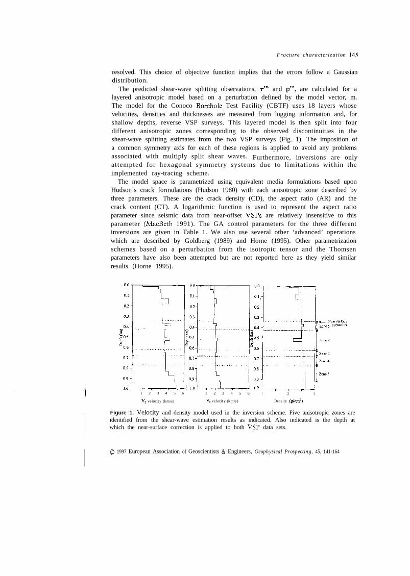
The predicted shear-wave splitting observations, 7m and pm, are calculated for alayered anisotropic model based on a perturbation defined by the model vector, m.The model for the Conoco Borehole Test Facility (CBTF) uses 18 layers whosevelocities, densities and thicknesses are measured from logging information and, forshallow depths, reverse VSP surveys. This layered model is then split into fourdifferent anisotropic zones corresponding to the observed discontinuities in theshear-wave splitting estimates from the two VSP surveys (Fig. 1). The imposition ofa common symmetry axis for each of these regions is applied to avoid any problemsassociated with multiply split shear waves. Furthermore, inversions are onlyattempted for hexagonal symmetry systems due to limitations within theimplemented ray-tracing scheme.
The model space is parametrized using equivalent media formulations based uponHudson’s crack formulations (Hudson 1980) with each anisotropic zone described bythree parameters. These are the crack density (CD), the aspect ratio (AR) and thecrack content (CT). A logarithmic function is used to represent the aspect ratioparameter since seismic data from near-offset VSPs are relatively insensitive to thisparameter (MacBeth 1991). The GA control parameters for the three differentinversions are given in Table 1. We also use several other ‘advanced’ operationswhich are described by Goldberg (1989) and Horne (1995). Other parametrizationschemes based on a perturbation from the isotropic tensor and the Thomsenparameters have also been attempted but are not reported here as they yield similarresults (Horne 1995).
1.0 .Il LO-LA---J 1.01 2 3 4 5 6 1 2 3 4 5 6
VP velocity (km/s) V, velocity (km/s)
1 2 3
Density (g/cm3)
Figure 1. Velocity and density model used in the inversion scheme. Five anisotropic zones areidentified from the shear-wave estimation results as indicated. Also indicated is the depth atwhich the near-surface correction is applied to both VW data sets.
0 1997 European Association of Geoscientists & Engineers, Geophysical Prospecting, 45, 141-164
146 S. Horne et al.
Table 1. GA inversion parameters.
GA Parameter
Population sizeNumber of generationsCrossover probabilityMutation probabilitySharingReordering (‘Inversion’)Hill climbing (‘G-bit improvement’)
NPOPNkm
PCPI-ll
6060
0.9500.010JJJ
Application to field data
The ray-tracing algorithm is incorporated into the GA which we then apply toinverting shear-wave splitting observations from two similar near-offset VSPexperiments. The near-offset VSP experiments were conducted at two differentwells within 1 km of each other at the CBTF. The site is located in north centralOklahoma in a relatively simple structural setting. The section penetrated by thewells consists of relatively flat-lying Permian and Pennsylvanian shales, limestones,and sandstones, as described by Queen and Rizer (1990).
Near-0fSset VSP acquisition geometries
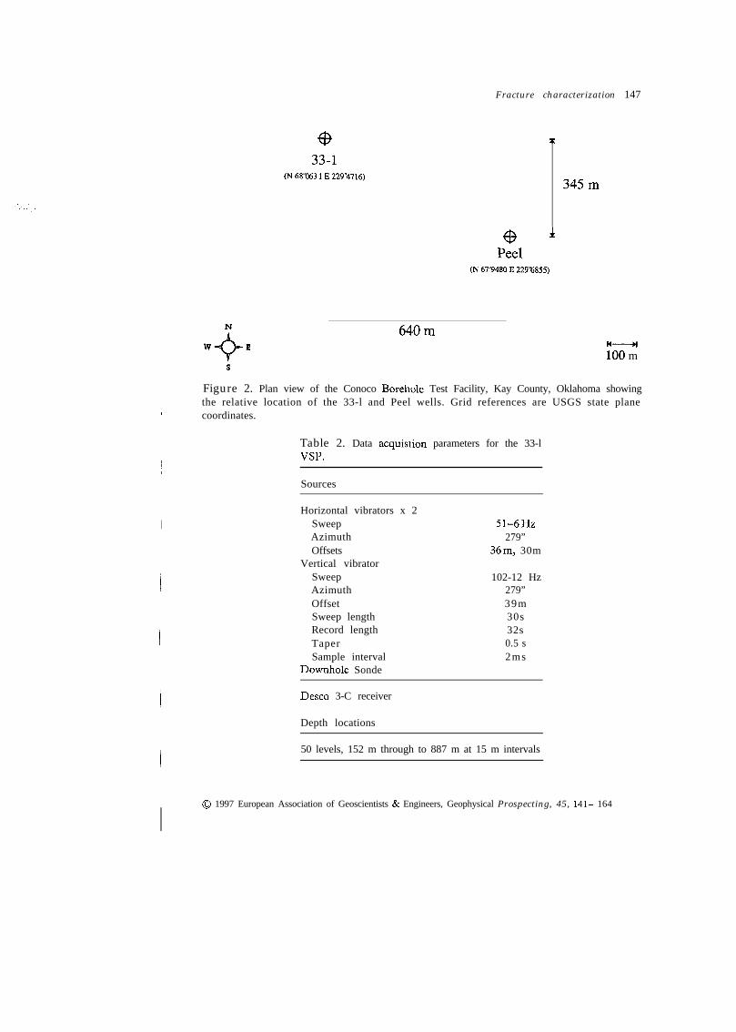
We identify the two near-offset VSPs as the 33-l VSP and the Peel VSP, referring tothe two wells about which the experiments were shot. The Peel well is locatedapproximately 740m to the south-east of well 33-l (Fig. 2). The acquisitiongeometries for these two experiments are similar in terms of the angles of incidencesampled, but the azimuthal propagation directions sampled correspond to almostdiametrically opposite raypaths. The importance of information obtained along suchopposite azimuths will become apparent and will be discussed in relation to verticaland non-vertical crack systems. A summary of the acquisition geometries and thesource and receiver parameters is given in Tables 2 and 3. Plan views of both VSPacquisition geometries are shown in Fig. 3.
3 3 - l VSP7. -i
;*- pVibroseis sources were located 36 m (120 ft) along the azimuth N279”E relative to .&;well 33-l. The Vibroseis sources were operated in in-line, cross-line and vertical ?G’;:directions. Seismograms were recorded at 50 levels between depths of 152 m (500 fi) $$ ~and 887m (2910 ft) using a constant geophone spacing of 15m (50 ft).horizontally polarized Vibroseis sources were swept through a frequency rangeto 51 Hz, whereas the vertically polarized vibrator was swept through a range of 1102 Hz.
0 199’7 European Association of Geoscientists & Engineers, Geophysical Prospecting, 4% 141
33-l(N 68%3 1 E 229’4716)
Fracture characterization 147
345 m
@ LPeel
(N 679480 E 229’6855)
640 m
iO0 m
Figure 2. Plan view of the Conoco Borehole Test Facility, Kay County, Oklahoma showingthe relative location of the 33-l and Peel wells. Grid references are USGS state planecoordinates.
Table 2. Data acquistion parameters for the 33-lVW.
Sources
Horizontal vibrators x 2SweepAzimuthOffsets
Vertical vibratorSweepAzimuthOffsetSweep lengthRecord lengthTaperSample interval
Downhole Sonde
51-6Hz279”
36m, 30m
102-12 Hz279”39m30s32s0.5 s2ms
Desco 3-C receiver
Depth locations
50 levels, 152 m through to 887 m at 15 m intervals
/ 0 1997 European Association of Geoscientists & Engineers, Geophysical Prospecting, 45, 141- 164

148 S. Home et al.
Table 3. Data acquisition parameters for the PeelVSP.
Sources
Horizontal vibrators x 2SweepAzimuthOffsets
Vertical vibratorSweepAzimuthOffsetSweep lengthRecord lengthTaperSample interval
Downhole Sonde
7-60 Hz122”65m
7-15 Hz123”71m14s15s0.2sl m s
GSC-20D 3-C receiver
Depth locations
44 levels, 306 m through to 951 m at 15 m intervals
33-l VSP
Vibroseis
Figure 3. Plan views showing the acquisition geometries used to obtain the multicomponentnear-offset VSP data sets.
-10 m
Peel VSP N
i
10m
0 1997 European Association of Geoscientists & Engineers, Geophysical Prospecting, 45, 141- 164
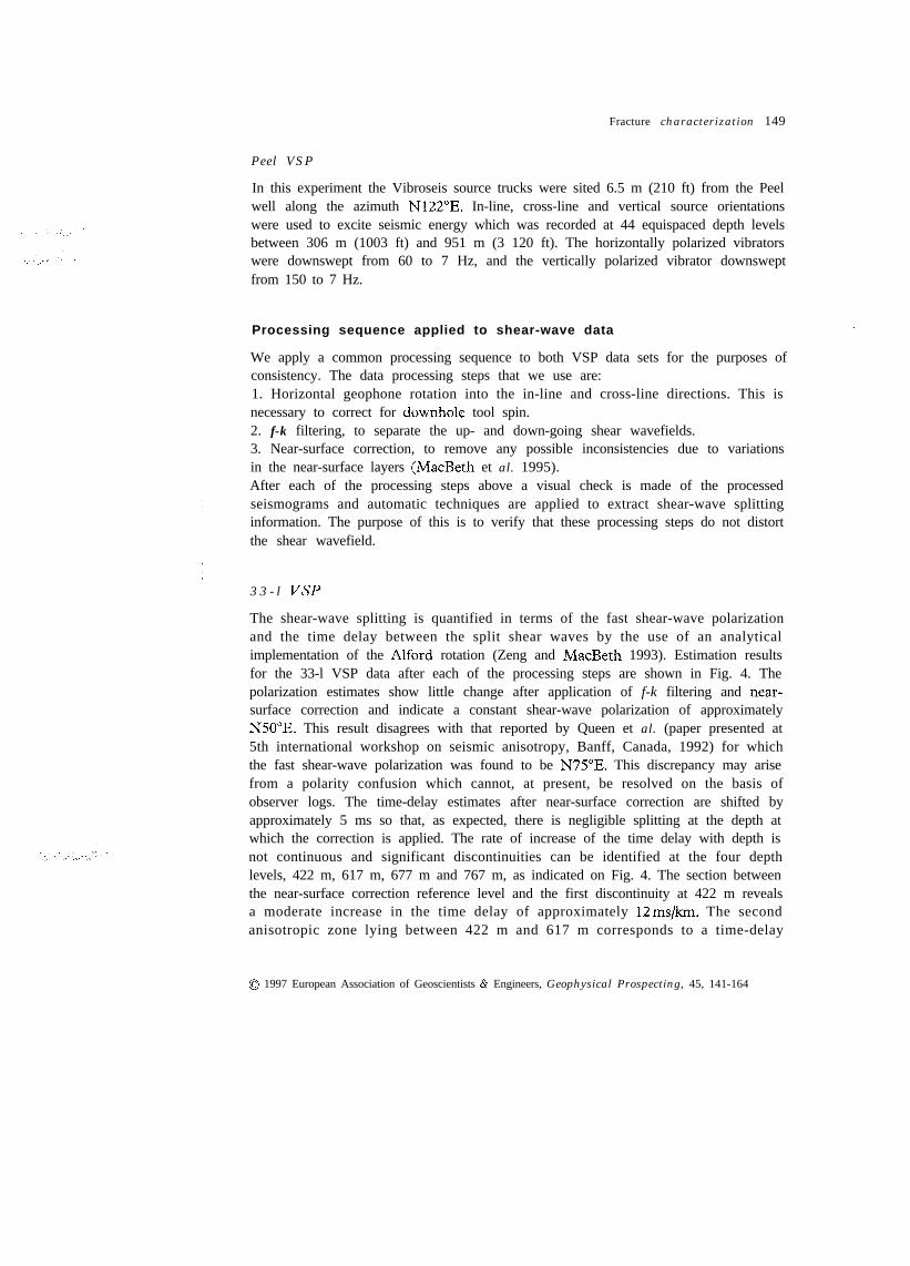
Fracture characterization 149
Peel VSP
In this experiment the Vibroseis source trucks were sited 6.5 m (210 ft) from the Peelwell along the azimuth N122”E. In-line, cross-line and vertical source orientationswere used to excite seismic energy which was recorded at 44 equispaced depth levelsbetween 306 m (1003 ft) and 951 m (3 120 ft). The horizontally polarized vibratorswere downswept from 60 to 7 Hz, and the vertically polarized vibrator downsweptfrom 150 to 7 Hz.
Processing sequence applied to shear-wave data
We apply a common processing sequence to both VSP data sets for the purposes ofconsistency. The data processing steps that we use are:1. Horizontal geophone rotation into the in-line and cross-line directions. This isnecessary to correct for downhole tool spin.2. f-k filtering, to separate the up- and down-going shear wavefields.3. Near-surface correction, to remove any possible inconsistencies due to variationsin the near-surface layers (MacBeth et al. 1995).After each of the processing steps above a visual check is made of the processedseismograms and automatic techniques are applied to extract shear-wave splittinginformation. The purpose of this is to verify that these processing steps do not distortthe shear wavefield.
3 3 - l VSP
The shear-wave splitting is quantified in terms of the fast shear-wave polarizationand the time delay between the split shear waves by the use of an analyticalimplementation of the Alford rotation (Zeng and MacBeth 1993). Estimation resultsfor the 33-l VSP data after each of the processing steps are shown in Fig. 4. Thepolarization estimates show little change after application of f-k filtering and near-surface correction and indicate a constant shear-wave polarization of approximatelyN50”E. This result disagrees with that reported by Queen et al. (paper presented at5th international workshop on seismic anisotropy, Banff, Canada, 1992) for whichthe fast shear-wave polarization was found to be N75”E. This discrepancy may arisefrom a polarity confusion which cannot, at present, be resolved on the basis ofobserver logs. The time-delay estimates after near-surface correction are shifted byapproximately 5 ms so that, as expected, there is negligible splitting at the depth atwhich the correction is applied. The rate of increase of the time delay with depth isnot continuous and significant discontinuities can be identified at the four depthlevels, 422 m, 617 m, 677 m and 767 m, as indicated on Fig. 4. The section betweenthe near-surface correction reference level and the first discontinuity at 422 m revealsa moderate increase in the time delay of approximately 12ms/km. The secondanisotropic zone lying between 422 m and 617 m corresponds to a time-delay
0 1997 European Association of Geoscientists & Engineers, Geophysical Prospecting, 45, 141-164

150 S. Home et al.
Zone 1
Zone 3
800900
Zone 5
lOOO-1 1ooo-~I0 30 60 90 120 150 180 0 10 20 30
qSI PolarizationT i m e delay (ms)
(Degrees N of E)
Figure 4. Shear-wave estimation results for the 33-l VSP at various processing stages.
gradient of 33 m&n. The third zone is apparently isotropic as there is noappreciable change in the time-delay estimates over this depth range. Between 677 mand 767m there is a significant increase in the time-delay gradient to 97ms/km.Below this depth range, the time-delay estimates decrease to a minima of 18ms at827 m and then increase to 23 ms for the deepest recording at 887 m.
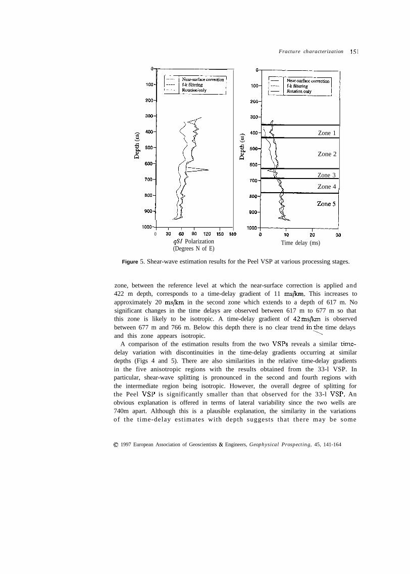
Peel VSP
Results from the application of shear-wave estimation techniques are shown in Fig.5. Unlike the results for the 33-l VW, the near-surface correction has a considerableeffect in clarifying the estimation results. Before near-surface correction theestimated qSI polarizations decrease steadily with depth from N90”E at shallowlevels to N60”E. After the correction this rotation becomes less apparent and the qS1polarizations are shifted towards N55”E. Before the near-surface correction there isno clear time-delay variation with depth as observed for the 33-l VSP estimationresults. None the less, possible discontinuities can be observed at depths similar tothose identified in the 33-l VW results. However, after the near-surface correctionthe time-delay gradients can be measured with more confidence. The first anisotropic
0 1997 European Association of Geoscientists & Engineers, Geophysical Prospecting, 45, 141-164
,.c-. ,
$&.
Fracture characterization 1
s
400,
g 500.
6600.
700-
800-
QOO-
lOOO- I I I I I0 30 60 90 120 150 160
qSI Polarization(Degrees N of E)
Zone 1
Zone 2
Zone 3
Zone 4
lOOO-))0 10 20 30
Time delay (ms)
Figure 5. Shear-wave estimation results for the Peel VSP at various processing stages.
zone, between the reference level at which the near-surface correction is applied and422 m depth, corresponds to a time-delay gradient of 11 mslkm. This increases toapproximately 20 ms/km in the second zone which extends to a depth of 617 m. Nosignificant changes in the time delays are observed between 617 m to 677 m so thatthis zone is likely to be isotropic. A time-delay gradient of 42ms/km is observedbetween 677 m and 766 m. Below this depth there is no clear trend in? time delaysand this zone appears isotropic.
A comparison of the estimation results from the two VSPs reveals a similar time-delay variation with discontinuities in the time-delay gradients occurring at similardepths (Figs 4 and 5). There are also similarities in the relative time-delay gradientsin the five anisotropic regions with the results obtained from the 33-l VSP. Inparticular, shear-wave splitting is pronounced in the second and fourth regions withthe intermediate region being isotropic. However, the overall degree of splitting forthe Peel VW is significantly smaller than that observed for the 33-l VW. Anobvious explanation is offered in terms of lateral variability since the two wells are740m apart. Although this is a plausible explanation, the similarity in the variationsof the time-delay estimates with depth suggests that there may be some
0 1997 European Association of Geoscientists & Engineers, Geophysical Prospecting, 45, 141-164
152 S. Horne et al.
correspondence between the observed anisotropy in the two wells. Furthermore, thetwo VSPs are shot in a relatively simple geological setting so that lateral changes areunlikely, although this possibility cannot be ruled out. The inversion results that weobtain show that such lateral changes need not be invoked to explain these shear-wave splitting observations.
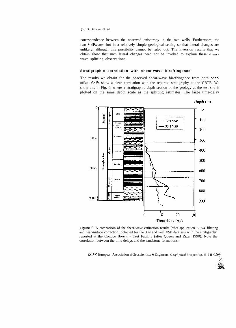
Stratigraphic correlation with shear-wave birefringence
The results we obtain for the observed shear-wave birefringence from both near-offset VSPs show a clear correlation with the reported stratigraphy at the CBTF. Weshow this in Fig. 6, where a stratigraphic depth section of the geology at the test site isplotted on the same depth scale as the splitting estimates. The large time-delay
C
300m
600ml
Wabaunsee
Depth (m)
Ki 11,
I I
500
600
700
800
900
0 10 20Time delay (ms)
30
Figure 6. A comparison of the shear-wave estimation results (after application off-K filteringand near-surface correction) obtained for the 33-l and Peel VSP data sets with the stratigraphyreported at the Conoco Borehole Test Facility (after Queen and Rizer 1990). Note thecorrelation between the time delays and the sandstone formations. I
0 199’7 European Association of Geoscientists & Engineers, Geophysical Prospecting, 45, 141-164 ‘:;
Fracture characterization 153
gradients for the two depth ranges 422-617 m and 677-767 m correspond toformations with considerable amounts of sandstone interbedded with shale. Thiscorrelation suggests that the shear-wave birefringence is sensitive to the presence ofopen fractures in the sandstones. The depth interval at 700 m has also been observedto correspond to fluid loss in all of the deep wells at the CBTF which is attributed tolarge open fractures within this zone (Queen et al. 1992, as above). Alternatively,these sandstone formations may exhibit preferential grain alignment due todepositional conditions leading to equivalent anisotropic behaviour (Helbig 1994).However, the coincidence of the qS1 polarizations with the maximum compressivestress direction (Zoback and Zoback 1980) suggests that the observed seismicanisotropy is not related to such depositional fabrics. Furthermore, examination ofcore samples from the test site do not indicate any depositional fabrics with therequired orientation to explain these observations (Queen and Rizer 1990).
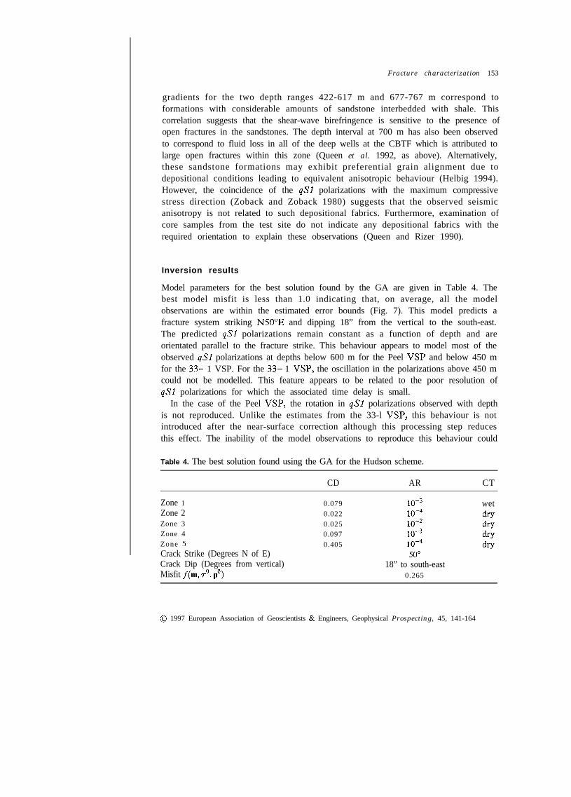
Inversion results
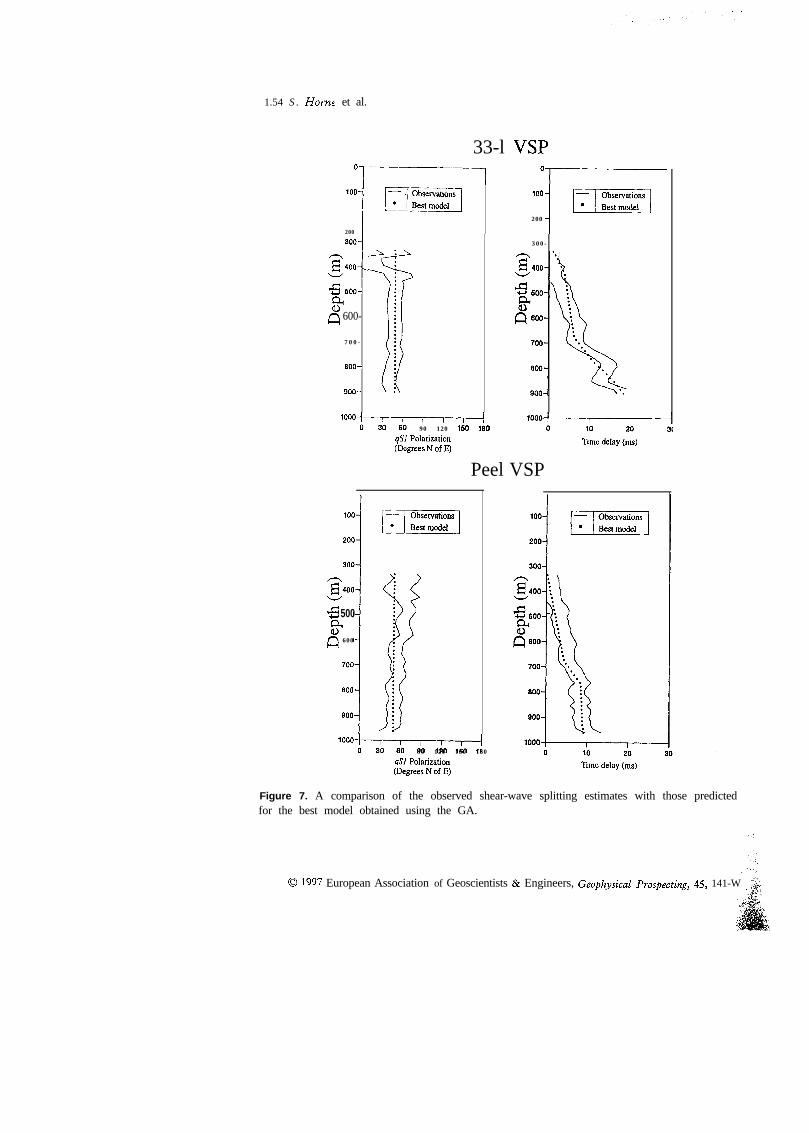
Model parameters for the best solution found by the GA are given in Table 4. Thebest model misfit is less than 1.0 indicating that, on average, all the modelobservations are within the estimated error bounds (Fig. 7). This model predicts afracture system striking N50”E and dipping 18” from the vertical to the south-east.The predicted qS1 polarizations remain constant as a function of depth and areorientated parallel to the fracture strike. This behaviour appears to model most of theobserved qSI polarizations at depths below 600 m for the Peel VW and below 450 mfor the 33- 1 VSP. For the 33- 1 VW, the oscillation in the polarizations above 450 mcould not be modelled. This feature appears to be related to the poor resolution ofqS1 polarizations for which the associated time delay is small.
In the case of the Peel VW, the rotation in qS1 polarizations observed with depthis not reproduced. Unlike the estimates from the 33-l VW, this behaviour is notintroduced after the near-surface correction although this processing step reducesthis effect. The inability of the model observations to reproduce this behaviour could
Table 4. The best solution found using the GA for the Hudson scheme.
CD AR CT
Zone 1 0.079 1o-2 wetZone 2 0.022 1o-4 dryZone 3 0.025 1o-2 dryZone 4 0.097 1O-3 dryZone 5 0.405 1o-4 dryCrack Strike (Degrees N of E) 50”Crack Dip (Degrees from vertical) 18” to south-eastMisfit f(m, TO, p”) 0.265
0 1997 European Association of Geoscientists & Engineers, Geophysical Prospecting, 45, 141-164
1.54 S. Home et al.
33-l VSP
OT-----7 “T-----‘00
200 1
-1 ‘00
1
-1200
300
2400A
32u 500-&Q 600-
700-
aoo-
900-
2;...............
i;
........
......
.
300-
90 120 160 180
qS1 Polarization(Degrees N of E)
Peel VSP
lime delay (ms)
L:* 5003Q 600
‘“OO,b90 120 150 180
aSI Polarization(Degrees N of E)
lime delay (ms)
Figure 7. A comparison of the observed shear-wave splitting estimates with those predictedfor the best model obtained using the GA.
0 1997 European Association of Geoscientists & Engineers, Geophysical Prospecting, 45, 141-W ~ ,,>i.a;+ ‘,

I
n
Fracture characterization 155
lie in the failure of the optimization method to converge or in the assumptionsemployed in the forward-modelling scheme. It is possible that the GA fails toconverge to a lower misfit value since there is no proof that such methods are able tofind the global minima. The alternative explanation of restrictive assumptions whichdo not allow a realistic representation of the problem is now addressed. Essentiallythere are three main assumptions used in the forward modelling. These are theapproximation of the geology at the test site to a 1D stack of plane layers, the use of aray method and the representation of the anisotropy as a transversely isotropicmedium with an arbitrary orientation of the symmetry axis which is constant withdepth. This first assumption is judged to be valid through the consideration ofgeological data from the CBTF. The second assumption of the ray-tracing methodappears justified through comparison tests with full waveform synthetics generatedusing the reflectivity method (Horne 1995). The remaining assumption of transverseisotropy may be inappropriate since horizontal fine layering and subverticalfracturing, both of which are likely to be present at the test site, lead to equivalentmedia of the monoclinic symmetry class. For these systems, at near-verticalpropagation directions the observed anisotropy will be dominated by the near-vertical fractures. On moving away from the vertical direction the fine layeringanisotropy becomes increasingly dominant and for some systems this leads to the qS1shear wave being polarized parallel to the radial direction. This combination ofsubvertical fracturing and fine layering anisotropy can be used to explain themeasured qS1 behaviour observed for both VSPs. For the 33-l VW, the source islocated along the azimuth N279”E. This implies that shear-wave energy ispropagating closer to the supposed fracture orientation of N50”E dipping 18” tothe south-east. This compares with the Peel VSP source which is locatedapproximately downdip along azimuth N122”E. Thus, the qS1 polarizationsobserved from the 33-l VSP will be dominated by the fracturing anisotropy,whereas the qS1 polarizations for the Peel VSP will be more sensitive to thefine-layering anisotropy. Equal area plots for the situations described are shown inFig. 8. Unfortunately, a forward-modelling scheme able to produce accurate resultsfor such monoclinic symmetry systems could not be efficiently implemented withinthe GA.
The majority of the predicted time delays fall within the estimated error boundsfor both VSPs (Fig. 7). The poorest agreement occurs in zone 5, below 800 m, for the33- 1 VW. In this zone the observed time delays decrease between 800 m and 850 mand increase below this depth. For this depth range the raypaths are essentiallyvertical with the straight line angles of incidence ranging between 2.4” and 2.6”.Since the angular variation is essentially the same over this interval it is unlikely thatthis variation is due to anisotropic propagation effects. Decreases in time delay can beexplained in terms of multiple splitting which may be caused by a change in thesymmetry system or its orientation. Such a change can be introduced through avariation in the fracture orientation with depth. However, the implemented ray-tracing scheme assumes there is no such change and this effect cannot be modelled
$.J 1997 European Association of Geoscientists & Engineers, Geophysical Prospecting, 45, 141-164

156 S. Home et al.
Horizontal tine layering Combination ofhorizontal fine layering
and dipping fractures
Figure 8. Lower-hemisphere equal-area plots showing the qS1 polarizations between anglesof incidence 0” and 30” for (a) a TIV medium constructed from horizontal fine layering, (b) aTI medium constructed from Hudson cracks dipping 24” to the south-east and strikingN50”E. (c) A monoclinic medium constructed by combining horizontal fine layering and thedipping crack systems shown in (a) and (b). Marked on this figure are the two angular aperturescorresponding to the Peel and 33-l VSPs. For the 33-l VSP, the qS1 polarizations are alignedwith the crack strike, whereas the polarizations measured using an aperture corresponding tothat used for the Peel VSP show a rotation towards the radial direction with increasingincidence.
with the present inversion scheme. It should be emphasized that this assumption isnecessary to construct an efficient forward-modelling scheme and is not a limitationof either ray tracing or the GA optimization scheme.
Non-uniqueness
The acceptable models, f(m, TO, p”) < 1 .O, sampled by the GA are shown in distance-misfit scatter plots (Fig. 9). For these plots, the multiparameter model vector isrepresented in terms of a single parameter, the distance D(m), which is essentially anormalized form of the vector magnitude. These plots allow a convenient visualizationof the sampling distribution of high-dimension parameter spaces. The problem isclearly non-unique and within this window of acceptable solutions there are 233 models.
Of particular interest is the non-uniqueness associated with the crack orientation.We show this by plotting the strike and dip for each of the acceptable models usinga scatter plot for which each dot is shaded according to that model’s misfit value(Fig. 10). The models are clustered about the best model between crack strikes ofN35”E and N65”E and crack dips between 10” and 40” to the south-east. The fracturedips for the better models are concentrated about values of approximately 20” to thesouth-east. This clustering is controlled by the time-delay observations. The reasonfor this can be clearly explained using Fig. 11, in which velocity sheets and lower-hemisphere equal-area plots of time delays are shown for equivalent anisotropicmedia constructed from vertical fractures and subvertical fractures. Referring to thecross-sections of both the velocity sheets and the time-delay plots in the plane
0 1997 European Association of Geoscientists & Engineers, Geophysical Prospecting, 45, 141-164

Fracture characterization
0 . 2 -
0.4-i
- !,y , ’.! :j.- -
8:
0;. .o-%
1
.“Ps 0.6 . .
.
. -. .. .
.. .--. -:.. . .z . . . -- - .-. ..- .-. -.. -.
--. -.,.- .
1.57
1.0 1 . . . .,.-: . --. . .,I
0.0 1.0 2.0 3.0 4.0 5.0Distance D(m)
Figure 9. Distance-misfit scatter plots showing models for which the misfit is less than 1.This misfit range corresponds to models whose observations, on average, fit all the observeddata within the estimated error bounds.
perpendicular to the crack strike, it can be seen that the seismic anisotropy for thedipping fractures is no longer symmetrical about the vertical axis. If we now considertwo near-offset VSPs with sources located along diametrically opposite azimuths,which is approximately the case for the Peel VSP and 33-l VSP, then the observedshear-wave birefringence is the same for vertical fracture anisotropy. However, forthe subvertical fracture system, the shear-wave birefringence is greater for the VSPtransmitting shear waves along the plane of fracturing than for the VSP on theopposite azimuth. This effect is observed in the two near-offset VSPs for which thetime delays are larger for the 33-l VSP compared with the Peel VSP. We proposethat this technique of opposite azimuth VSP surveys may be of significant use in thediscrimination and measurement of subvertical fracture systems.
Resolution
We calculate the model parameter resolution by computing misfit values along cross-sections through the model space about the best solution. We achieve this bysweeping through one component of the model vector whilst keeping all othercomponents equal to the best model parameters. The resolution for each parameter iscalculated using a measure of dispersion, a, given by
I
112(%,best - %)2L(f) , (3)
0 1997 European Association of Geoscientists & Engineers, Geophysical Prospecting, 45, 141-164
158 S. Home et al.
24:
0
3 lo-
20 -
30 - mNE!
40 -I I
N NE E SE SCrack stride
Misfit j@z,$, p”)
f,(m,z”, p”)=O.265
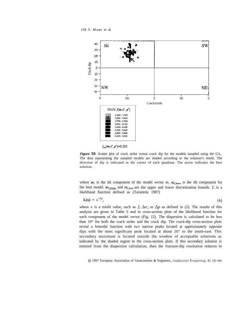
Figure IO. Scatter plot of crack strike versus crack dip for the models sampled using the GA.The dots representing the sampled models are shaded according to the solution’s misfit. Thedirection of dip is indicated in the corner of each quadrant. The arrow indicates the bestsolution.
where m; is the ith component of the model vector m. %?i,best is the ith component forthe best model. %%?i,high and mi,loW are the upper and lower discretization bounds. L is alikelihood function defined as (Tarantola 1987)
L(x) = e-h,
where x is a misfit value, such as f, Ar, or Ap as defined in (2). The results of thisanalysis are given in Table 5 and in cross-section plots of the likelihood function foreach component of the model vector (Fig. 12). The dispersion is calculated to be lessthan 10” for both the crack strike and the crack dip. The crack-dip cross-section plotsreveal a bimodal function with two narrow peaks located at approximately oppositedips with the most significant peak located at about 20” to the south-east. Thissecondary maximum is located outside the window of acceptable solutions asindicated by the shaded region in the cross-section plots. If this secondary solution isomitted from the dispersion calculation, then the fracture-dip resolution reduces to
0 1997 European Association of Geoscientists 2% Engineers, Geophysical Prospecting, 45, 141-164

Vertical cracks
3.25
3 2.75
3
+l 2.50 -.Z
5:
> 73
2.25 -
1.75 t-90
,-60
(-30 ,0 30 60 bo
Degrees from vertical
3.25
- 2.75VI
B
;? 2 . 5 0.t:
Fracture characterization
Dipping cracksI
159
f 2.25
2.MJ
L-l
9SI
9s2
1.75 J-90 -60 -30 0 30 60 90
Degrees from vertical
Figure 1 I . A comparison of anisotropic behaviour for materials constructed from vertical(left) and subvertical (right) fractures. The subvertical cracks are rotated 20” from the vertical.The lower plots show the time-delay variations over a hemisphere of propagation directionswith the inner circle indicating an equi-incident angle of 10”.
less than 1”. To identify the source of this secondary solution, cross-section plotsare constructed for the separate time-delay and qS1 polarization misfit terms in (2)(Fig. 13). The crack dip cross-section reveals that the contribution from the qSIpolarization misfit is essentially constant between dips of f 25”. Beyond this rangethe likelihood function rapidly decreases to zero. This cut-off is due to the rapidchanges in the predicted qSI observations which occur for these large values of dip asthe line singularity is sampled. The time-delay likelihood function is bimodal withwell-defined peaks at dips of 18” to the south-east and 24” to the north-west. The
0 1997 European Association of Geoscientists & Engineers, Geophysical Prospecting, 45, 141- 164
160 S. Horne et al.
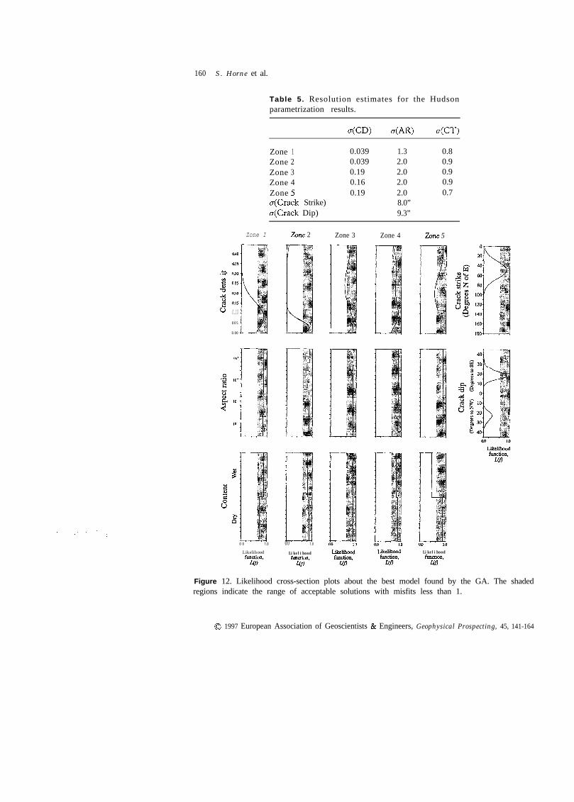
Table 5. Resolution estimates for the Hudsonparametrization results.
dCD> 4W 4CT)
Zone 1Zone 2Zone 3Zone 4Zone 5a(Crack Strike)a(Crack Dip)
0.039 1.3 0.80.039 2.0 0.90.19 2.0 0.90.16 2.0 0.90.19 2.0 0.7
8.0”9.3”
Zone I Zone 2
04003s
b.z 0.302 0.25-224 0.200 015c3 0.10
0 0 5
0.00
0 0 1.0 0 0 1.0
Likelihood Likelihoodfilnction.
wliEtiOIl.
47
Zone 3 Zone 4 Zone 5
0.0 I.0
Likelihoodfulclion,
uJ7
Figure 12. Likelihood cross-section plots about the best model found by the GA. The shadedregions indicate the range of acceptable solutions with misfits less than 1.
0 1997 European Association of Geoscientists & Engineers, Geophysical Prospecting, 45, 141-164
Fracture characterization 161
NO"E
N2O=E
N40"E
Q) N80"E22$j NlOO%
0
N120-E
N140"E
0.0 0.2 0.4 0.6 0.8
Likelihood function, L1.0 0.0 0.2 0.4 0.6 0.8
Likelihood function, L
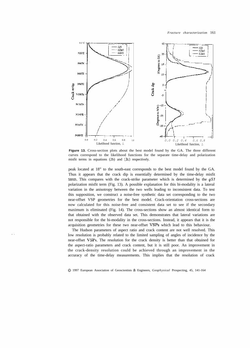
Figure 13. Cross-section plots about the best model found by the GA. The three differentcurves correspond to the likelihood functions for the separate time-delay and polarizationmisfit terms in equations (2b) and (2~) respectively.
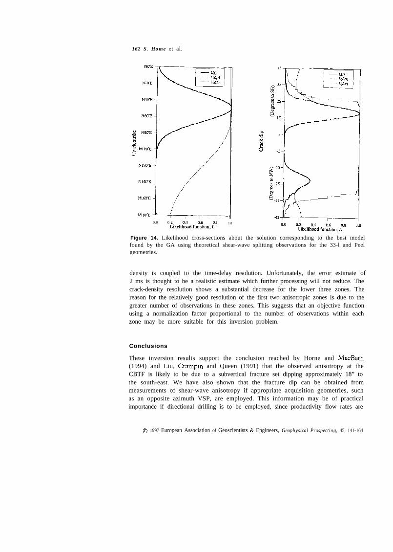
peak located at 18” to the south-east corresponds to the best model found by the GA.Thus it appears that the crack dip is essentially determined by the time-delay misfitterm. This compares with the crack-strike parameter which is determined by the qS1polarization misfit term (Fig. 13). A possible explanation for this bi-modality is a lateralvariation in the anisotropy between the two wells leading to inconsistent data. To testthis supposition, we construct a noise-free synthetic data set corresponding to the twonear-offset VSP geometries for the best model. Crack-orientation cross-sections arenow calculated for this noise-free and consistent data set to see if the secondarymaximum is eliminated (Fig. 14). The cross-sections show an almost identical form tothat obtained with the observed data set. This demonstrates that lateral variations arenot responsible for the bi-modality in the cross-sections. Instead, it appears that it is theacquisition geometries for these two near-offset VSPs which lead to this behaviour.
. -The Hudson parameters of aspect ratio and crack content are not well resolved. This
low resolution is probably related to the limited sampling of angles of incidence by thenear-offset VSPs. The resolution for the crack density is better than that obtained forthe aspect-ratio parameters and crack content, but it is still poor. An improvement inthe crack-density resolution could be achieved through an improvement in theaccuracy of the time-delay measurements. This implies that the resolution of crack
0 1997 European Association of Geoscientists 81 Engineers, Geophysical Prospecting, 45, 141-164
162 S. Home et al.
NO=E
N20-E
N40”E
0.0 0.2LikelilEd fu2km, I!‘*
1.0
Figure 14. Likelihood cross-sections about the solution corresponding to the best modelfound by the GA using theoretical shear-wave splitting observations for the 33-l and Peelgeometries.
density is coupled to the time-delay resolution. Unfortunately, the error estimate of2 ms is thought to be a realistic estimate which further processing will not reduce. Thecrack-density resolution shows a substantial decrease for the lower three zones. Thereason for the relatively good resolution of the first two anisotropic zones is due to thegreater number of observations in these zones. This suggests that an objective functionusing a normalization factor proportional to the number of observations within eachzone may be more suitable for this inversion problem.
Conclusions
These inversion results support the conclusion reached by Horne and MacBeth(1994) and Liu, Crampin and Queen (1991) that the observed anisotropy at theCBTF is likely to be due to a subvertical fracture set dipping approximately 18” tothe south-east. We have also shown that the fracture dip can be obtained frommeasurements of shear-wave anisotropy if appropriate acquisition geometries, suchas an opposite azimuth VSP, are employed. This information may be of practicalimportance if directional drilling is to be employed, since productivity flow rates are
0 1997 European Association of Geoscientists & Engineers, Geophysical Prospecting, 45, 141-164
Fracture characterization 163
maximized for wells perpendicularly intersecting the fractures. Furthermore, anunderstanding of the fracture system’s dip is also important with respect to thereservoir’s structural behaviour, since this controls the water-cut behaviour ofproducing wells.
A significant correlation is observed to exist between the lithology at the CBTFand the shear-wave birefringence. Specifically, the degree of birefringence isconsiderably higher in the formations dominated by sandstones, suggesting that theseformations may be intensely fractured. Sandstone formations, such as the SpraeberryField, Texas, are of importance to the petroleum industry since they may often be thelocation of hydrocarbon reservoirs (Aguilera 1980). For these reservoirs the formationpermeability anisotropy is of essential importance to production. Therefore shear-wave birefringence studies may prove to be useful in these situations.
Acknowledgements
S.Horne thanks ELF GRC and the sponsors of the Edinburgh Anisotropy Projectfor their financial support. This work was supported by the Natural EnvironmentResearch Council, and is published with the approval of the director of the BritishGeological Survey.
References
Aguilera R. 1980. Naturally Fractured Reservoirs. PennWell Publishing Company, Tulsa,Oklahoma.
Ata E. and Michelena R.J. 1995. Mapping distributions of fractures in a reservoir with P-Sconverted waves. The Leading Edge 14, 664-676.
Cervenjr V. 1972. Seismic rays and ray intensities in inhomogeneous anisotropic media.Geophysical Journal of the Royal Astronomical Society 29, 1 - 13.
Crampin S. and Love11 J.H. 1991. A decade of shear-wave splitting in the Earth’s crust: whatdoes it mean? what use can we make of it? and what should we do next? Geophysical JournalInternational 107, 387-408.
Davis L. 1991. Handbook of Genetic Algorithms. Van Nostrand Reinhold, New York.Ehlig-Economides C., Ebbs D. and Meehan D.N. 1990. Factoring anisotropy into well design.
Oiljield Review (October) 24-33.Fogel D.B. and Stayton L.C. 1994. On the effectiveness of crossover in simulated evolutionary
optimization. BioSystems 32, 171-182.Fryer G.F. and Frazer L.N. 1987. Seismic waves iri stratified anisotropic media -11.
Elastodynamic eigensolutions for some anisotropic systems. Geophysical Journal of the RoyalAstronomical Society 91, 73-101. ‘_
Gajewski D. and PSenEik I. 1990. Vertical seismic profile synthetics by dynamic ray tracingin laterally varying layered anisotropic structures. Journal of Geophysical Research 95,11301-l 1315.
Goldberg D.E. 1989. Genetic Algorithms in Search, Optimization, and Machine Learning.Addison-Wesley Pub. Co.
0 1997 European Association of Geoscientists & Engineers, Geophysical Prospecting, 45, 141-164

164 S. Horne et al.
Helbig K. 1994. Foundations of Anisotropy for Exploration Seismics. Elsevier SciencePublishing Co.
Horne S. 1995. Applications of genetic algorithms to problems in seismic anisotropy. Ph.D thesis,University of Edinburgh.
Horne S. and MacBeth C. 1994. Inversion for seismic anisotropy using genetic algorithms.Geophysical Prospecting 42, 953-974.
Hudson J.A. 1980. Overall properties of a cracked solid. Mathematical Proceedings of theCambridge Philosophical Society 88, 371-384.
Li Y.G., Leary P.C. and Aki K. 1990. Ray series modelling of seismic wave travel times andamplitudes in three-dimensional heterogeneous anisotropic crystalline rock: Boreholevertical seismic profiling seismograms from the Mojave Desert, California. Journal ofGeophysical Research 95, 11225- 11239.
Liu E., Crampin S. and Queen J.H. 1991. Fracture detection using crosshole surveys andreverse vertical seismic profiles at the Conoco Borehole Test Facility, Oklahoma.Geophysical Journal International 107, (3), 449-463.
MacBeth C. 1991. Inversion for subsurface anisotropy using estimates of shear-wave splitting.Geophysical Journal International 107, 585-595.
MacBeth C., Zeng X., Li X.-Y. and Queen J. H. 1995. Multicomponent near-surfacecorrection for land VSP data. Geophysical Journal International 121, 301-315.
Mueller M. 1992. Using shear waves to predict lateral variability in vertical fracture intensity.The Leading Edge 12, 29-35.
Musgrave M. J.P. 1970. Crystal Acoustics. Holden-Day, Inc.Pereya V., Lee W.H.K. and Keller H.B. 1980. Solving two point seismic ray tracing in a
heterogeneous medium, Prt I: A general adaptive finite difference method. Bulletin of theSeismological Society of America 70, 79-99.
Press W.H., Teukolsky S.A., Vetterling W.T. and Flannery B.P. 1992. Numerical Recipes inFortran: The Art of Scientific Computing. Cambridge University Press.
Queen J.H. and Rizer W.D. 1990. An integrated study of seismic anisotropy and the naturalfracture system at the Conoco Borehole Test Facility, Kay County, Oklahoma. Journal ofGeophysical Research 95, 11255- 11273.
Sen M.K. and Stoffa P.L. 1992. Rapid sampling of model space using genetic algorithms:examples from seismic waveform inversion. GeophysicalJournal International 108,281-292.
Tarantola A. 1987. Inverse Problem Theory: Methods for Data Fitting and Model ParameterEstimation. Elsevier Science Publishing Co.
Zeng X. and MacBeth C. 1993. Algebraic processing techniques for estimating shear-wavesplitting in zero-offset VSPs - theory. Geophysical Prospecting 41, 1033-1066.
Zoback M.L. and Zoback M. 1980. State of stress in the conterminous United States. Journalof Geophysical Research 85, 6113-6156.
0 1997 European Association of Geoscientists & Engineers, Geophysical Prospecting, 45, 141-164