Chopra S 3D VSP Processing and Integration VSP-1

8/2/2019 Chopra S 3D VSP Processing and Integration VSP-1

http://slidepdf.com/reader/full/chopra-s-3d-vsp-processing-and-integration-vsp-1 1/4

1

3D VSP – processing and integration with surface seismic Satinder Chopra, Emil Blias, Lioudmila Chavina, Vlaidmir Alexeev and Glen Larsen - Scott Pickford

Abhi Manerikar and Andrew Kryzan - Conoco Canada Resources Ltd

Introduction

Ever since the first 3D vertical seismic profile (VSP) acquisition was experimented in 1986 by AGIP, several 3D VSP volumes have beenacquired [1-9]. Apart from the 3D VSP acquisition, a simultaneous VSP and 3D surface seismic acquisition has been attempted [10], andthe results have been encouraging in terms of cost effectiveness and the enhanced imaging of the subsurface.

This work is an attempt to describe the simultaneous acquisition of 3D surface seismic data, the 3D VSP data and to detail the differentsteps that were followed to process the two data volumes. Attempts were made to enhance the bandwidth of the 3D seismic data usingthe VSP downgoing wavefield and integrate the 3D VSP volume with surface seismic to be able to interpret the two together.

Acquisition of data

Simultaneous data acquisition of surface 3D and 3component 3D VSP data was carried out by Crestar Energy Ltd. (now Conoco), inOctober 2000 in Hanna area in Central Alberta. The geometry used for the 3D survey is the Mega Bin TM typical staggered brick patternwith a source spacing 70 m and a receiver spacing 140 m, sample rate 1 ms, record length 3 s and the energy source was dynamite.Using the same seismic source, and an 80 level (using Paulsson Geophysical tool), 3 component geophone cable in well 8-20, data wassimultaneously recorded on the surface and the borehole. This acquisition represented approximately 3000 shots.

The 3D seismic programs (surface and VSP) were recorded to assist in defining sand presence and porosity development in the LowerMannville interval (Ellerslie SS) found at a depth of between 1300.0 and 1350.0m. The 3D VSP recording was expected to (a) to help tiethe seismic reflections to lithology and stratigraphic boundaries, (b) yield a high frequency image around the borehole (the fixed receiverarray and its proximity to the reservoir are expected to improve image quality), and (c) help determine an improved subsurface velocitymodel.

Processing of 3D seismic data

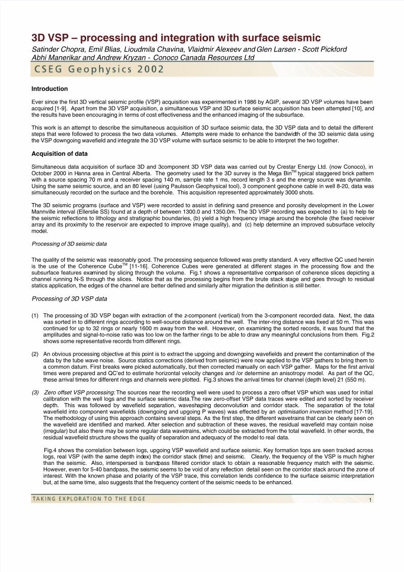
The quality of the seismic was reasonably good. The processing sequence followed was pretty standard. A very effective QC used hereinis the use of the Coherence Cube TM [11-16]. Coherence Cubes were generated at different stages in the processing flow and thesubsurface features examined by slicing through the volume. Fig.1 shows a representative comparison of coherence slices depicting achannel running N-S through the slices. Notice that as the processing begins from the brute stack stage and goes through to residualstatics application, the edges of the channel are better defined and similarly after migration the definition is still better.

Processing of 3D VSP data

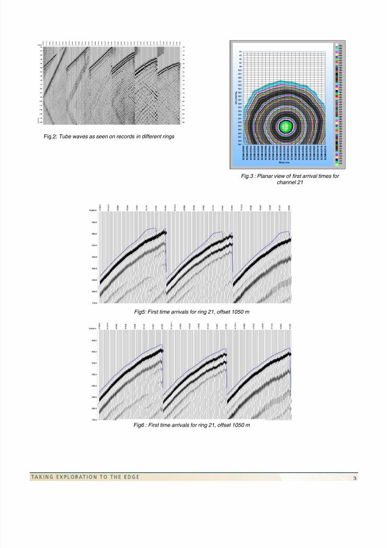
(1) The processing of 3D VSP began with extraction of the z-component (vertical) from the 3-component recorded data. Next, the datawas sorted in to different rings according to well-source distance around the well. The inter-ring distance was fixed at 50 m. This wascontinued for up to 32 rings or nearly 1600 m away from the well. However, on examining the sorted records, it was found that theamplitudes and signal-to-noise ratio was too low on the farther rings to be able to draw any meaningful conclusions from them. Fig.2shows some representative records from different rings.

(2) An obvious processing objective at this point is to extract the upgoing and downgoing wavefields and prevent the contamination of thedata by the tube wave noise. Source statics corrections (derived from seismic) were now applied to the VSP gathers to bring them toa common datum. First breaks were picked automatically, but then corrected manually on each VSP gather. Maps for the first arrivaltimes were prepared and QC’ed to estimate horizontal velocity changes and /or determine an anisotropy model. As part of the QC,these arrival times for different rings and channels were plotted. Fig.3 shows the arrival times for channel (depth level) 21 (550 m).

(3) Zero offset VSP processing: The sources near the recording well were used to process a zero offset VSP which was used for initial

calibration with the well logs and the surface seismic data.The raw zero-offset VSP data traces were edited and sorted by receiverdepth. This was followed by wavefield separation, waveshaping deconvolution and corridor stack. The separation of the totalwavefield into component wavefields (downgoing and upgoing P waves) was effected by an optimisation inversion method [17-19].The methodology of using this approach contains several steps. As the first step, the different wavetrains that can be clearly seen onthe wavefield are identified and marked. After selection and subtraction of these waves, the residual wavefield may contain noise(irregular) but also there may be some regular data wavetrains, which could be extracted from the total wavefield. In other words, theresidual wavefield structure shows the quality of separation and adequacy of the model to real data.

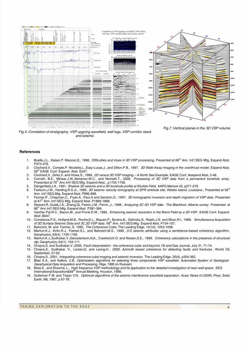
Fig.4 shows the correlation between logs, upgoing VSP wavefield and surface seismic. Key formation tops are seen tracked acrosslogs, real VSP (with the same depth index) the corridor stack (time) and seismic. Clearly, the frequency of the VSP is much higherthan the seismic. Also, interspersed is bandpass filtered corridor stack to obtain a reasonable frequency match with the seismic.However, even for 5-40 bandpass, the seismic seems to be void of any reflection detail seen on the corridor stack around the zone ofinterest. With the known phase and polarity of the VSP trace, this correlation lends confidence to the surface seismic interpretationbut, at the same time, also suggests that the frequency content of the seismic needs to be enhanced.



2

(4) Offset VSP processing: Travel time inversion was used to create a layered anisotropic velocity model for each ring. To begin with, anisotropic layered velocity model was created from zero offset VSP first arrivals. This model consisted of 18 layers with thethicknesses ranging from 50 to 150 m. For different offsets, the first arrivals were calculated and overlayed on the real data. As seenin Fig.5, the isotropic velocity model derived from zero offset VSP first arrivals does not fit offset data. To get a better match, ananisotropic layered velocity model is used. For each ring, a vertical axis of anisotropy is considered with elliptical anisotropyassociated with each layer. The elliptic anisotropy coefficients V H /VV (VH = horizontal velocity, and V V = vertical velocity) aredetermined by minimizing the difference between real first break time values and those of the model. The minimum of a misfitfunction was found by using a Monte Carlo approach (global optimisation) first and then local optimisation. After going through thisexercise the average difference between the real and model arrivals is less than 1.5 ms. Fig.6 shows the actual wavefield and modelfirst breaks for the anisotropic model. For different rings the anisotropic coefficients were found to be between 0.85 and 1.15 and in

the shallow part rises to 1.25.

(5) The velocity model so generated was used to calculate the upgoing and multiple downgoing travel times, to put them into each VSPgather and help during wavefield separation for each ring.

(6) The total wavefield was separated into component wavefields, i.e. downgoing, upgoing, downgoing tubewaves and upgoingtubewaves.

(7) VSP deconvolution (for both downgoing and upgoing wavefields). This helped in restoring frequencies of upgoing wavefield using thedowngoing wavefield.

(8) A close look at the downgoing and the upgoing wavefields, revealed an interesting observation. The wavelets embedded in these datado not appear to be uniform. This set us thinking about the causes of the non-uniformity in the wavelets. We plotted the shot pointdepth and found that there is a significant oblique N-S trend in the depth pattern and is not uniform. To try and equalize theembedded source wavelets, a matched filtering was done between a model wavelet and the embedded source wavelets in the data.This enabled us to have a globally consistent wavelet in the data. The model wavelet was chosen as the average source wavelet inthe consistent zones.

(9) VSP-CDP time-to-depth transformation for every ring was done to obtain vertical VSP profiles. For this, the velocity modeldetermined in step 4 was used. Next, all depth images were stacked after making automatic time shift determination. This preventsany loss of higher frequencies and a crisp image was obtained for different offsets.

(10) Stacking of ring images (with time shifts) to obtain a 3D VSP volume, still in depth.

(11) Depth to time transformation and integrating with 3D VSP volume. Some vertical planes cutting through the 3D VSP time volume maybe seen in Fig.7. This volume was then merged with the seismic volume

Conclusions

The processing of 3D VSP was an enriching experience, though quite labour intensive and time consuming. The vertical profiles throughthe 3D VSP volume exhibited higher resolution and so detailed and focussed reflections, especially at the target level. The deployment of

a large number of borehole seismic receivers was expected to yield a larger reflection coverage around the borehole and seems to havepaid off here. The results of this project have demonstrated the benefit of the integrated approach pursued which seeks to optimise the setexploration objectives.

The experience gained through processing, integrating the two data sets recorded simultaneously and evaluating the final results permit usto recommend that such simultaneous surveys conducted at an incremental cost (so commercially feasible) could provide detailed imagessought around the borehole.

Acknowledgements

Mega Bin is a trademark of PanCanadian Petroleum and Coherence Cube is a trademark of Core Laboratories.

We would like to thank Conoco Canada Resources for release of data and thank both Conoco Canada Resources and Scott Pickford,Canada for permission to publish this paper. Authors from Scott Pickford wish to thank Vasudhaven Sudhakar for constantencouragement and helpful discussions.

After brute stack After residual statics After migration

Fig.1: Coherence time slices at different stages of processing

984 ms 984 ms 984 ms



3

Fig.3 : Planar view of first arrival times for channel 21

Fig5: First time arrivals for ring 21, offset 1050 m

Fig6 : First time arrivals for ring 21, offset 1050 m

Fig.2: Tube waves as seen on records in different rings



4

References

1. Boelle,J.L., Kaiser,P. Maocec,E., 1998, Difficulties and clues in 3D VSP processing , Presented at 68 th Ann. Int’l SEG Mtg. Expand Abst.P373-376.

2. Clochard,V., Compte,P. Nicoletis,L.,Svay-Lucas,J., and Dillon,P.B., 1997, 3D Walk-Away Imaging in the overthrust model , Expand Abst.59 th EAGE Conf. Expand. Abst. E047.

3. Clochard,V., Dirks,V. and Howe,S., 1999, 2D versus 3D VSP imaging – A North Sea Example , EAGE Conf. Aexpand.Abst. 2-48.4. Cornish, B.E., Minear,J.W.,Kempner,W.C., and Nemeth,T., 2000, Processing of 3D VSP data from a permanent borehole array ,

Presented at 70 th Ann.Int’l SEG Mtg. Expand Abst., p1755-1758.5. Dangerfield,J.A., 1991, Shallow 3D seismic and a 3D borehole profile at Ekofisk Field, AAPG Memoir 42, p271-279.6. Fairborn,J.W., Harding,R.S.Jr., 1996 , 3D seismic velocity tomography at SPR sinkhole site, Weeks Island, Louisiana , Presented at 59 th

Ann. Int’l SEG Mtg. Expand Abst. P896-898.7. Farmer,P., Chapman,C., Fryer,A., Paul,A and Sandvin,O., 1997, 3D tomographic inversion and depth migration of VSP data , Presented

at 67 th Ann. Int’l SEG Mtg. Expand Abst. P1866-1868.8. Stewart,R.,Gulati,J.S., Zhang,Qi, Parkin,J.M., Peron.,J., 1998 , Analyzing 3C-3D VSP data: The Blackfoot, Alberta survey. Presented at

68 th Ann.Int’l SEG Mtg. Expand Abst. P381-384.9. VanDer Pal,R.C., Bacon,M., and Pronk,D.W., 1995, Enhancing seismic resolution in the Brent Field by a 3D VSP , EAGE Conf. Expand.

Abst .B047.10. Constance,P.E., Holland,M.B., Roche,S.L., Biquart,P., Byrans,B., Gelinsky,S., Ralph,J.G. and Bloor,R.I., 1999, Simultaneous Acquisition

of 3D Surface Seismic Data and 3C,3D VSP data , 69 th Ann. Int’l SEG Mtg. Expand Abst. P104-107.11. Bahorich, M. and Farmer, S. 1995, The Coherence Cube , The Leading Edge, 14(10), 1053-1058.12. Marfurt,K.J., Kirlin,R.J., Farmer,S.L. and Bahorich,M.S., 1998 , 3-D seismic attributes using a semblance-based coherency algorithm ,

Geophysics, 63(4), 1150-1165.13. Marfurt,K.J.,Sudhakar,V.,Gersztenkorn,N,A., Crawford,K.D. and Nissen,S.E., 1999, Coherency calculations in the presence of structural

dip , Geophysics, 64(1), 104-111.

14. Chopra,S. and Sudhakar,V ,2000, Fault interpretation - the coherence cube and beyond , Oil and Gas Journal, July 31, 71-74.15. Chopra,S., Sudhakar, V., Larsen,G. and Leong,H. , 2000, Azimuth based coherence for detecting faults and fractures , World Oil ,September, 57-62.

16. Chopra,S., 2001, Integrating coherence cube imaging and seismic inversion, The Leading Edge, 20(4), p354-362.17. Blias E.A., and Katkov, U.B. Optimization algorithms for selecting three components VSP wavefield. Automated System of Geological-

Geophysical Data Acquisition and Processing , Riga, 1990 (in Russian)18. Blias,E., and Shavina, L., High frequency VSP methodology and its application to the detailed investigation of near-well space , SEG

International Exposition&69 th Annual Meeting, Houston, 1999.19. Goltsman F.M. and Trojan V.N., Optimum algorithms of the seismic interference wavefield separation , Acad. News of USSR, Phys. Solid

Earth, N8, 1967, p 67-78.

Fig.4: Correlation of stratigraphy, VSP upgoing wavefield, well logs, VSP corridor stack and seismic

Fig.7: Vertical planes in the 3D VSP volume

Documents

Chopra S 3D VSP Processing and Integration VSP-1