Ind

ust

rial E

lectr

ical En

gin

eerin

g a

nd

A

uto

matio

n

CODEN:LUTEDX/(TEIE-5299)/1-74/(2012)

Dynamic BrakingFPGA Implementation of DCC

Måns AnderssonAleksandar Stojkovic

D of Industrial Electrical Engineering and Automation Lund University

I

II

Dynamic Braking FPGA implementation of a DCC

Måns Andersson Aleksandar Stojkovic

June 2012

Supervisor: Yury Loayza

Examinor: Professor Mats Alaküla

Master’s  Thesis Division of Industrial Electrical Engineering and Automation

III

IV

Abstract In this thesis a Direct Current Control (DCC) is implemented for controlling a PMSM. The

controller should be implemented in an already existing program. This program is used for

testing electrical machines. The new testing method is called Dynamic braking, more

information about this method can be read in the report "Performance and efficiency

evaluation of FPGA controlled IPMSM under dynamic loading," by Y. Loayza, A. Reinap

and M. Alaküla.

The reason to implement a DCC is that the current PI-controller have problems with sudden

changes in current reference. This has become a limitation of the speed due to the risk of

damaging the inverter. With the characteristics of a DCC some of the problems that a PI-

controller can be neglected, for example the need of feedforwarding and overshoots. Also the

simplicity of the DCC is an advantage. This comes with a cost which is that it demands high

sampling frequency. But with the FPGA’s parallel execusion and possibility to high sampling

frequency it is possible to use the DCC.

The goal of this thesis is to make the DCC work in the existing project and also take care of

the problem that the previous controller had.

The implemented DCC was able to work in the existing project. A new problem has occurred,

the switching frequency. Due to the fact that the DCC is switching when needed, the

switching frequency can be too high , this limits the minimum size of the tolerance band. The

things that has to be considered in the choise of tolerance band is the switching frequency

against the control of the current. Smaller tolerance band gives better control to the cost of

higher switching frequency. With the DCC the influence of cogging is reduced in the

measurement and the control of the current is improved.

V

VI

Sammanfattning I detta examensarbete har en toleransbandsstryning (Direct current control, DCC)

implementerats i en befintlig styrning för permanent magnetiserade elektriska motorer,

styrningen används för en ny testmetod för elektiska motorer. Den nya tesmetoden kallas

”Dynamisk Bromsning”, mer information om denna metod kan läsas i rapporten

"Performance and efficiency evaluation of FPGA controlled IPMSM under dynamic loading,"

by Y. Loayza, A. Reinap and M. Alaküla.

DCC:n implmenterades av anledningen att den befintliga PI-kontrollern har problem med

snabba ändringar av strömreferensen. Detta har inneburit en begränsning av hastigheten

eftersom det finns risk att skada omriktaren. De två olika kontrollmetoderna har olika

karakteristik där DCC är den enklare, vilket gör den mindre känslig. Däremot kräver den

snabbare datainsamling för att kunna reglera bra. Denna höga insamlings hastighet kan

uppnås med en FPGA-enhet med insticksmoduler.

Målet med arbetet har varit att utveckla och implementera DCC styrningen i projketet, och få

den till fungera ihop med existerande delar.

Den nya styrningen fungerade bra i det befintliga projektet, men det uppkom ett problem,

switchfrekvensen. Till skillnad mot PI-kontrollern som har en fast frekvens så reglerar DCC

när det behövs. Är då tolerancebanden för små blir switchfrekvens högre än vad omriktaren

klarar. Större toleranceband innebör lägre switchfrekvens men samtidigt blir strömregleringen

sämre, det är en fråga om vad som prioriteras. Med DCC reglering så miskar koggingens

påverkan på strömmätningarna och regleringen blir bättre.

VII

VIII

Acknowledgment Thanks to everybody at the institution for a great time. Especially to Getachew Darge for all

the help with the hardware and all the tips and tricks along the way. Also big thanks to our

supervisor Yury Loayza for all the help with especially LabView and for all the good and

helpful discussions during the whole process from starting with the simulations to the finished

controller. We want to thank Project Eldrivet for an interesting and inspiring day in

Gothenburg. Thanks to Pelle Steen at National Instruments that also helped a lot with the

LabView, especially at the start when learning to use the program. Last but definitely not least

we want to thank Mats Alaküla for giving us the project and also for the help and inspiration

during the project.

We also want to thank Sebastian, Gabriel and Eric for the fun and entertaining time at the

“Fika”-breaks!

Lund, June 2012

Aleksandar and Måns

IX

1

Table of contents 1 INTRODUCTION ....................................................................................................................................... 3

1.1 BACKGROUND ............................................................................................................................................... 3

1.1.1 Goals ................................................................................................................................................ 5

2 THEORY ................................................................................................................................................... 6

2.1 THEORY OF DYNAMIC TESTING .......................................................................................................................... 6

2.2 VOLTAGE LIMITATION ..................................................................................................................................... 9

2.3 PERMANENT MAGNETIZED ELECTRIC MACHINES THEORY ........................................................................................ 9

2.4 CURRENT CONTROL ...................................................................................................................................... 12

FIGURE 5 - A MAP OF A CONTROL SYSTEM ..................................................................................................... 13

2.5 DCC ......................................................................................................................................................... 17

2.5.1 The Small Lookup table ................................................................................................................. 19

2.5.2 The Big lookup table ...................................................................................................................... 20

2.5.3 The hexagon .................................................................................................................................. 21

2.5.4 Example for the DCC ...................................................................................................................... 23

3 IMPLEMENTATION ................................................................................................................................ 26

3.1 DCC DEVELOPMENT ..................................................................................................................................... 26

3.2 BLANKING TIME ........................................................................................................................................... 27

3.3 FPGA ....................................................................................................................................................... 28

3.4 SWITCHING FREQUENCY ................................................................................................................................ 29

3.5 IMPLEMENTATION ........................................................................................................................................ 29

3.5.1 PC .................................................................................................................................................. 30

3.5.2 RT................................................................................................................................................... 30

3.5.3 FPGA .............................................................................................................................................. 30

3.6 HARDWARE SETUP ....................................................................................................................................... 32

4 RESULTS ................................................................................................................................................ 33

4.1 TEST SEQUENCE ........................................................................................................................................... 33

4.2 SMALL LOOKUP TABLE VS. BIG LOOKUP TABLE .................................................................................................... 35

4.2.1 The small lookup-table .................................................................................................................. 35

4.2.2 The big lookup-table ...................................................................................................................... 37

2

4.2.3 Comparison of the results .............................................................................................................. 39

4.3 DCC VS. PI ................................................................................................................................................. 39

4.4 POST PROCESSING RESULTS ............................................................................................................................ 47

5 CONCLUSION AND FURTHER DEVELOPMENT ........................................................................................ 51

5.1 LOOKUP-TABLES .......................................................................................................................................... 51

5.2 DCC ......................................................................................................................................................... 51

5.3 FURTHER DEVELOPMENTS .............................................................................................................................. 52

6 REFERENCES .......................................................................................................................................... 54

7 APPENDIX ............................................................................................................................................. 55

3

1 Introduction In the modern society more things are powered by electrical motors. The main reason is the

high energy efficiency and absence of exhaust emissions of the electrical motor. Since fossil

energy cost is increasing and environmental concerns are getting stronger the number of

electrically driven vehicles is growing. The politic goals are focused on the climate and how

to slow down the global warming. An emission intensive sector is the transport sector [1]. By

introducing in a first step hybrid vehicle and further on electric vehicles, a way of reducing

the emission of climate gases can be reached.

The expanding electrification of the transport sector leads to more researches and

development, which also means more testing and analyzing of electric machines and drives.

With the existing equipment the testing and evaluation is time consuming and the temperature

is not constant which creates uncertainties in the results.

This calls for a more effective way of measuring the characteristics of electric machines. With

faster measurement system a new opportunity of testing machines is made possible, that can

be done in just a couple of minutes and without removing the machine completely.

1.1 Background The development of control and measurement electronics towards higher speed/shorter

sampling intervals does not only provide better control possibilities, but also a chance to

measure and analyze the voltages dynamically supplied to and currents consumed by the

electrical machine. Today this can be done fast enough to provide measurement data collected

from a dynamic machine state, like an acceleration, that afterwards can be used to extract

detailed information of the machine. This information can be magnetic fluxes, torque, losses

etc. as a function of currents, speed, temperature etc.

This thesis is a part of the development of this novel testing method. A further development of

the control system and post-processing of measured data.

4

In the novel testing method called Dynamic Braking developed by IEA at LTH a vector

control system is used for current controlling based on PI-controllers and carrier wave

modulation. This method has shown problems related to controlling high current at high

speeds which has resulted in limitations on the speed in the testing cycle. The problem with

losing control over a high current can result in burned fuses and in worst case scenario it

could burn down the components of the power electronics. In an attempt to fix this problem a

Direct Current Controller (DCC) is implemented to evaluate how the faster dynamics of this

controller is able to handle the sudden changes of the current reference compared to the

previous PI-based controller. Because of the problem of sudden change in current, the top

speed of the test is reduced to be sure that none of the components or measurement equipment

is damaged.

Figure 1 - Power flow in a PMSM [2, p. 2]

Since this is a new method of testing electrical machines the post-processing of the measured

data needs to be furthered developed. The first step to do this is to make a better testing cycle

to be able to collect important data for later post-processing. To be able to do this the machine

has to be able to run throughout a wider speed-spectrum, which the DCC is implemented to

make possible.

5

1.1.1 Goals

This Master Thesis’s goals is to develop an alternative current controller to the PI-controller

in the Dynamic breaking project. The current controller should be implemented to work in the

project in parallel with the PI-controller. The updated post-processing program in Matlab

should continue to work with both current controllers. The specified goals are:

A further developed test method. o Developing a working DCC for a PMSM machine in LabView o Implement  the  controller  in  the  existing  project  “Dynamic  braking  “  as  an  

alternative to the existing PI-controller o Compare the characteristics of the implemented DCC with the existing PI-

controller o Adapt the existing post-processing method using Matlab to work with the

measured data from DCC o Further develop the post-processing in terms of finding the overall losses,

specify the order of the specific losses and calculate the efficiency of the machine

6

2 Theory In this chapter the theory behind the test method is explained. Also the theories behind the

things that is important to know to understand how the test method is constructed to work.

Some things are explained thoroughly while other things are mentioned so that the reader can

understand the context in the text. The most basic facts can be read in the Power Electronics

book [3].

2.1 Theory of Dynamic testing When testing an electric machine a test bench is needed with peripheral equipment like

braking motor, gearbox and torque sensor, see Figure 2. For testing a machine an important

thing is to line up everything to eliminate vibrations, which also take some time. The principal

of this method is that the machine accelerates with a specified current and uses the big

braking motor to hold a specified speed. When equilibrium is reached values are read. This

way of testing takes a lot of time and the machine gets warmer with every cycle. The

temperature rise is not negligible so this has to be compensated for later on [4].

Figure 2 - Traditional test bench. From left; big braking motor, gearbox, torque sensor and in the rear cornet the tested machine

7

The new testing approach does not need a test bench or other external equipment. The test

equipment can be mobile and the machine can be tested where it is placed by decoupling it

from the load [5].

This method can be done in two different environments:

The lab-environment where the machine is powered by the power electronics in the

lab. It is not critical that the measurement equipment is small since the lab offers

bigger space and the equipment is not moved often from the lab.

The in-situ environment which means that the test can be done anywhere. This is

possible because an electric vehicle has its own power supply and the idea of this test

method is to use that power supply for providing DC-voltage and also use the vehicles

power electronics to control the motor during the test.

The actual test is done by going through a set of different current references, this test

method is fast so the machine does not get significantly warmer. All the processing is

done using MATLAB after the test, so called post processing.

8

The Newton laws of physics also apply to electric machines and via them it is possible to

calculate the force (1), to do this the mass of the rotating parts of the machine and the

acceleration has to be known. The inertia can be calculated by doing acceleration cycles with

at least two different known weights coupled on the axis and then interpolate the points [4].

From the force it is possible to calculate the mechanic power (2) to (5).

𝐹 = 𝑚 ∙ 𝑎 ⇒ Τ = J ∙ 𝑎 (1)

�̇� = �̇� ∙2𝜋

𝑛polepair (2)

Τ =𝑑(J ∙ 𝜔)

𝑑𝑡 (3)

Assuming the inertia is constant.

Τ = �̇� ∙J (4) 𝑃 = Τ ∙ 𝜔 (5)

The electric power is much easier to calculate because the machine is controlled by different

voltage vectors and the current is used as feedback via current transducer modules.

𝑝 = 𝑢 ∙ 𝑖 + 𝑢 ∙ 𝑖 (6) When accelerating the machine the friction force is opposed the acceleration and vice versa

when braking the machine. To calculate the friction loss in the machine the acceleration part

with constant current reference is searched for. Acceleration is calculated as the derivative of

the electric speed, the same is for the deceleration part. The difference in slope is the friction

loss, and to have the loss in Nm the electric frequency is changed to  rad/𝑠 .

L =J

𝑛 ∙ 4 ∙ 𝜋(�̇� − �̇� ) (7)

9

2.2 Voltage limitation The machine should be accelerated to as high speed as it can get with each specific current

reference. To have some power to brake there must be enough difference between the induced

voltage (emf) and the highest stator voltage the supply is able to provide. From the pulse

references to the transistors it is possible to calculate how much time each transistor is on. If

the transistor is on half the time, half the DC-supply voltage is unused and can be used for

changing the speed reference. When the emf is as big as the DC-supply the controllability of

the machine is zero and the controller needs to lower the speed reference until the induced

voltage is smaller than the DC-supply.

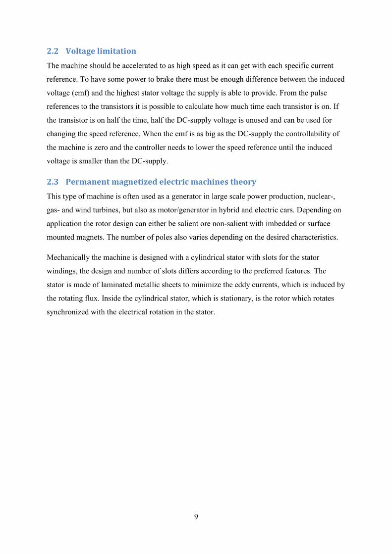
2.3 Permanent magnetized electric machines theory This type of machine is often used as a generator in large scale power production, nuclear-,

gas- and wind turbines, but also as motor/generator in hybrid and electric cars. Depending on

application the rotor design can either be salient ore non-salient with imbedded or surface

mounted magnets. The number of poles also varies depending on the desired characteristics.

Mechanically the machine is designed with a cylindrical stator with slots for the stator

windings, the design and number of slots differs according to the preferred features. The

stator is made of laminated metallic sheets to minimize the eddy currents, which is induced by

the rotating flux. Inside the cylindrical stator, which is stationary, is the rotor which rotates

synchronized with the electrical rotation in the stator.

10

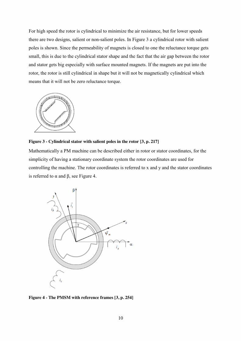
For high speed the rotor is cylindrical to minimize the air resistance, but for lower speeds

there are two designs, salient or non-salient poles. In Figure 3 a cylindrical rotor with salient

poles is shown. Since the permeability of magnets is closed to one the reluctance torque gets

small, this is due to the cylindrical stator shape and the fact that the air gap between the rotor

and stator gets big especially with surface mounted magnets. If the magnets are put into the

rotor, the rotor is still cylindrical in shape but it will not be magnetically cylindrical which

means that it will not be zero reluctance torque.

Figure 3 - Cylindrical stator with salient poles in the rotor [3, p. 217]

Mathematically a PM machine can be described either in rotor or stator coordinates, for the

simplicity of having a stationary coordinate system the rotor coordinates are used for

controlling the machine. The rotor coordinates is referred to x and y and the stator coordinates

is referred to α and β, see Figure 4.

Figure 4 - The PMSM with reference frames [3, p. 254]

11

The machine in stator references looks like

𝑢 = 𝑅 ∙ 𝚤 +𝑑𝜓𝑑𝑡 = 𝑅 ∙ 𝚤 +

𝑑𝑑𝑡 𝜓 + 𝐿 ∙ 𝚤 (8)

For the simplicity of having the references stationary the same can be written in rotor

coordinates and looks like.

𝑢 = 𝑅 ∙ 𝚤 +𝑑𝜓𝑑𝑡 = 𝑅 ∙ 𝚤 +

𝑑𝑑𝑡 𝜓 + 𝐿 ∙ 𝚤 + 𝑗𝜔 𝜓 + 𝐿 ∙ 𝚤 (9)

This can also be expressed in its components as

𝑢 = 𝑅 ∙ 𝑖 +𝑑𝑑𝑡

𝜓 + 𝑖 ∙ (𝐿 + 𝐿 ) − 𝜔 ∙ 𝑖 ∙ 𝐿 + 𝐿

= 𝑅 ∙ 𝑖 +𝑑𝑑𝑡

(𝜓 + 𝐿 ∙ 𝑖 ) − 𝜔 ∙ 𝐿 ∙ 𝑖 (10)

𝑢 = 𝑅 ∙ 𝑖 +𝑑𝑑𝑡 𝑖 ∙ 𝐿 + 𝐿 + 𝜔 ∙ 𝜓 + 𝑖 ∙ (𝐿 + 𝐿 )

= 𝑅 ∙ 𝑖 + 𝐿 ∙𝑑𝑖𝑑𝑡 + 𝜔 ∙ (𝜓 + 𝐿 ∙ 𝑖 )

(11)

The flux is also relative rotor shape and therefore it is divided to x and y part, as below.

𝜓 = 𝜓 + 𝐿 ∙ 𝑖 = 𝜓 + 𝑖 ∙ (𝐿 + 𝐿 )𝜓 = 𝐿 ∙ 𝑖 = 𝑖 ∙ 𝐿 + 𝐿                       (12)

The 𝐿 part is the main inductance in the x, y-direction, the difference is big with salient

poles and vice versa. The 𝐿 term is the stator leakage which is equal in all directions

because the stator is equally shaped.

Torque is a function of current and flux and is also dependent of how the rotor is shaped and

how the magnets are placed.

𝑇 = 𝜓 × 𝚤 = 𝜓 ∙ 𝑖 − 𝜓 ∙ 𝑖 = (𝜓 + (𝐿 + 𝐿 ) ∙ 𝑖 ) ∙ 𝑖 − 𝐿 + 𝐿 ∙ 𝑖 ∙ 𝑖

= 𝜓 ∙ 𝑖 + 𝐿 − 𝐿 ∙ 𝑖 ∙ 𝑖 (13)

The second part of the equations shows how the torque is dependent on the difference in

reluctance in the x and y-direction, this characteristic is used for torque controlling the

machine. By enhance the flux in the x-direction it is possible to make the machine stronger

and by adding negative x-current, field weakening it is possible to weaken the flux and make

the machine spin faster.

12

When dealing with electrical machines is important to have in mind the fact that one electric

turn is not always one mechanical turn therefore the number of magnetic poles has to be

known.

2.4 Current Control This chapter will give the basic information and comparison between a DCC and a PI-

controller. Some characteristics that are relevant to this project will be discussed. How the

two controllers are built up and how they work can be read in the Power Electronics book [3].

To be able to control an electrical machine the currents to the machine has to be known. The

currents can be described in different ways. Two of the systems have static coordinates, which

means that the currents are measured relative the stator. In the abc-frame the currents are

called after the phases, a, b and c. The phase differences between the currents are 120°. In the

αβ-frame which also is a stationary coordinate systems. The differences between the currents

are 90° in this case. Both describes the same currents but in different ways. The third way is

to represent the currents is the xy-frame. This frame is unlike the two previous following the

rotor. Like the αβ-frame the difference between the currents is 90°. This is also a way to

describe the same current as the abc- and αβ-frame but instead relative the rotor. The only

difference between the αβ-frame and the xy-frame is the position (angle) of the rotor in the

machine. In Figure 4 the three reference frames are illustrated in a PMSM-structure.

13

With the three reference frames from Figure 8 the phase current can be described as vectors in

any of the reference frames, how this is done is described in the Power electronics book [3].

The current vector is an easier and more illustrative way to represent a current. The same

current vector can be represented in all three reference frames the only difference will be how

the current is represented. The reason the currents are described in different ways is because

how they are used. For modulation it is easier to represent the current in abc-frame, while a

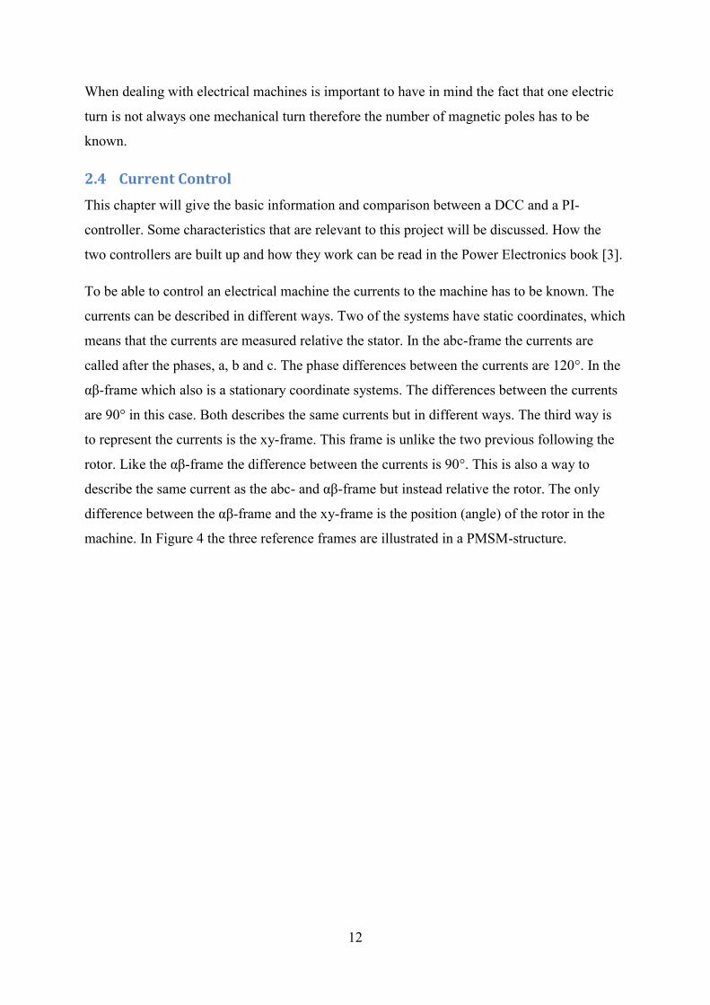
reference value for a regulator is easier described in xy- or αβ-frame. In Figure 5 a control

system is illustrated with the conversion between the different frames.

Figure 5 - A map of a control system

The different steps in Figure 5 are described in detail below:

1. The input to the regulation is given in xy-frame as a vector.

2. The output of the regulator is then converted, first into αβ-frame, this first step is

because it is mathematically easier to do the conversion xy - αβ - abc than to go direct

from xy to abc.

3. And finally from αβ to abc-frame to modulation. This conversion is made because the

modulation is giving the output of phases that corresponds to the abc-frame.

4. The current is measured in the three phases.

5. The current is then first converted from the abc-frame to the αβ-frame and finally

converted to the xy-frame to be able to compare the difference between the current

reference and the measured current.

In the implemented version of the dynamic braking a PI-controller is used. The problem with

the PI-controller is that sudden changes in current cause problems such as losing the control

of the current at high speeds. This can lead to burned fuses and in worst cases the power

electronics can be damaged. The reason that the PI-controller has these problems can be the

characteristics of the controller.

14

A PI-control tries to predict the voltage that the machine will need in the next future sampling

interval, based on a machine model with some degree of simplification. The current controller

is based on this simplification and does not account for e.g. cogging torque, induced voltages

due to harmonic frequencies etc. This is not wrong, but this causes problems for the controller

and results in a loss of control of the current at high speeds or sudden changes. The problem

with high speeds is that in one sampling interval there is a big change in the rotor angle. This

makes it hard for the PI-controller to make a good correction.

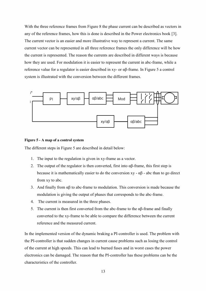
Another issue that can damage the power electronic components is the overshooting that

occurs when the current reference is changed, see Figure 6. This is typical characteristics for a

PI-controller that can be modified by choosing a good proportional- and integral-gain, but still

with high currents the problem can only be mitigated.

Figure 6 - Example of a overshooting

A good thing about the PI-controller is that the sampling frequency does not have to be

extremely fast. The measurement could have been done with equipment that has lower

sampling-frequency, in the range of a few kHz is enough. This is due to that the PI-controller

is modeled and constructed to predict potential faults and irregularities. The switching-

frequency is fixed due to the carrier wave. In this case the switching-frequency is set to

10 kHz.

15

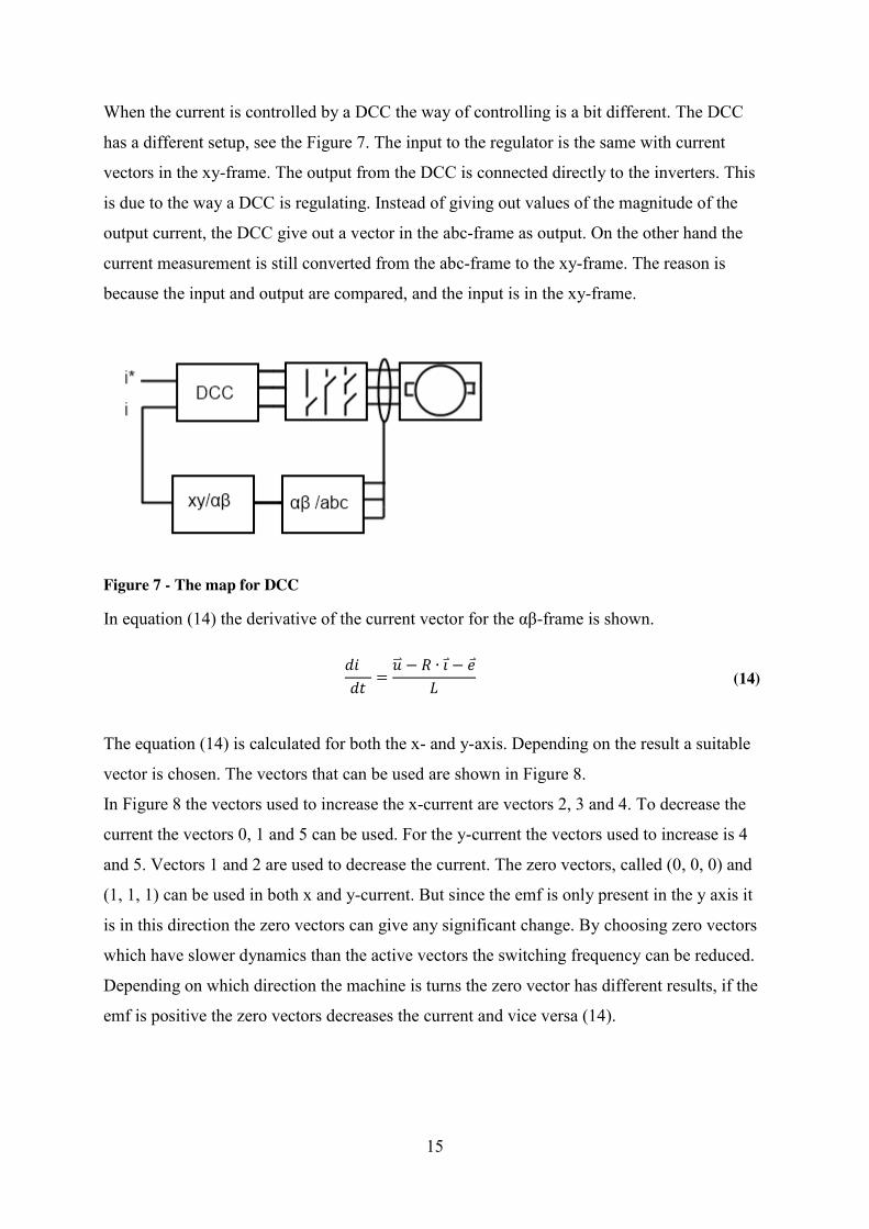
When the current is controlled by a DCC the way of controlling is a bit different. The DCC

has a different setup, see the Figure 7. The input to the regulator is the same with current

vectors in the xy-frame. The output from the DCC is connected directly to the inverters. This

is due to the way a DCC is regulating. Instead of giving out values of the magnitude of the

output current, the DCC give out a vector in the abc-frame as output. On the other hand the

current measurement is still converted from the abc-frame to the xy-frame. The reason is

because the input and output are compared, and the input is in the xy-frame.

Figure 7 - The map for DCC

In equation (14) the derivative of the current vector for the αβ-frame is shown.

𝑑𝑖𝑑𝑡 =

𝑢 − 𝑅 ∙ 𝚤 − 𝑒𝐿 (14)

The equation (14) is calculated for both the x- and y-axis. Depending on the result a suitable

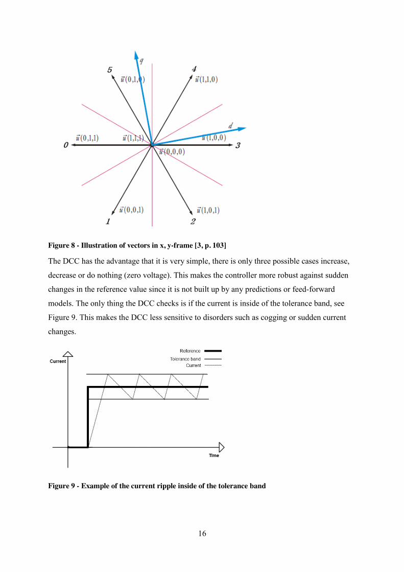
vector is chosen. The vectors that can be used are shown in Figure 8.

In Figure 8 the vectors used to increase the x-current are vectors 2, 3 and 4. To decrease the

current the vectors 0, 1 and 5 can be used. For the y-current the vectors used to increase is 4

and 5. Vectors 1 and 2 are used to decrease the current. The zero vectors, called (0, 0, 0) and

(1, 1, 1) can be used in both x and y-current. But since the emf is only present in the y axis it

is in this direction the zero vectors can give any significant change. By choosing zero vectors

which have slower dynamics than the active vectors the switching frequency can be reduced.

Depending on which direction the machine is turns the zero vector has different results, if the

emf is positive the zero vectors decreases the current and vice versa (14).

16

Figure 8 - Illustration of vectors in x, y-frame [3, p. 103]

The DCC has the advantage that it is very simple, there is only three possible cases increase,

decrease or do nothing (zero voltage). This makes the controller more robust against sudden

changes in the reference value since it is not built up by any predictions or feed-forward

models. The only thing the DCC checks is if the current is inside of the tolerance band, see

Figure 9. This makes the DCC less sensitive to disorders such as cogging or sudden current

changes.

Figure 9 - Example of the current ripple inside of the tolerance band

17

The drawback of the DCC is instead the switching-frequency. There are some small things to

have in mind to minimize these problems [6, p. 7]. Since it changes vectors when the current

is outside of the tolerance band the switching’s can be made whenever the controller needs to.

This means that it can be both more and less than 10 kHz which in our case is the

recommended maximum switching frequency. When it is below the limit there is no problem,

but when it exceeds this limit it can damage the transistors. One solution is to make the

tolerance band big enough so the changes, or switching’s, do not occur that often. Another is

to introduce double tolerance band that gives the opportunity to use passive vectors.

The reason why this DCC has not been used before is that no equipment has had the high

sampling-frequency required to handle a DCC. Before the sampling-frequency was in the

region of a few  kHz, and since the switching frequency is in the same range this would not

work. But with the Field-Programmable Gate Array (FPGA) the sampling frequency is in the

MHz [7] area and the opportunity to use a DCC is possible.

2.5 DCC When using a DCC the only thing one can change is the width of the tolerance band. In this

thesis both the x- and y-axis is controlled at the same time and the limits of the tolerance band

will look like a box in the x, y-frame, see Figure 10. For simplicity, first an explanation for a

control over one axis will be explained, and then how to put them together.

Figure 10 - The tolerance band for the x, y-currents

First of all, a decision has to be made if only the active vectors should be available or if the

passive vectors also should be used. The difference is that if the passive vectors are used

correctly the switching frequency will be lowered. To be able to use the passive vector, an

outer tolerance band has to be implemented. The reason is that the controller needs to know if

18

it can use the passive vector or it has to use an active vector. To understand how this works an

example is written in chapter 2.5.4.

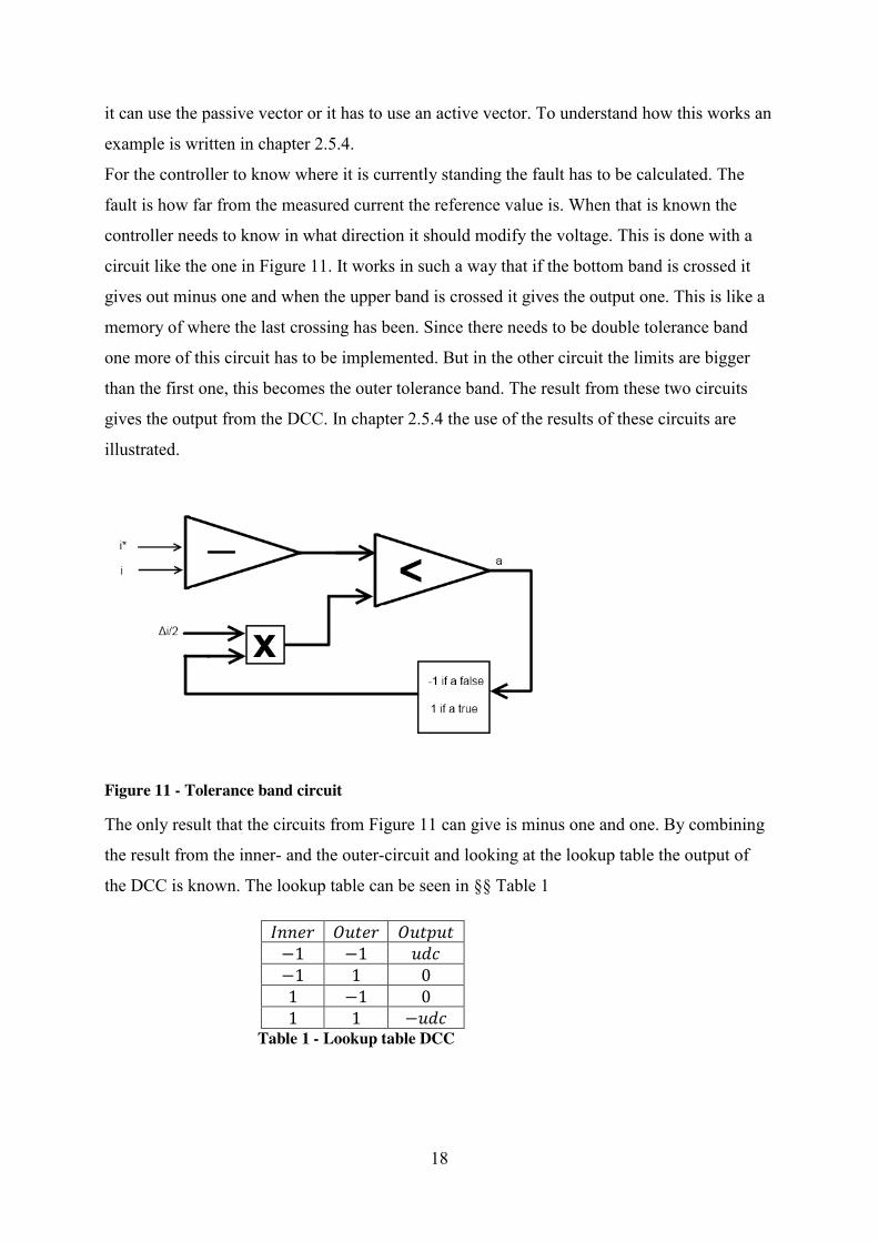
For the controller to know where it is currently standing the fault has to be calculated. The

fault is how far from the measured current the reference value is. When that is known the

controller needs to know in what direction it should modify the voltage. This is done with a

circuit like the one in Figure 11. It works in such a way that if the bottom band is crossed it

gives out minus one and when the upper band is crossed it gives the output one. This is like a

memory of where the last crossing has been. Since there needs to be double tolerance band

one more of this circuit has to be implemented. But in the other circuit the limits are bigger

than the first one, this becomes the outer tolerance band. The result from these two circuits

gives the output from the DCC. In chapter 2.5.4 the use of the results of these circuits are

illustrated.

Figure 11 - Tolerance band circuit

The only result that the circuits from Figure 11 can give is minus one and one. By combining

the result from the inner- and the outer-circuit and looking at the lookup table the output of

the DCC is known. The lookup table can be seen in §§ Table 1

𝐼𝑛𝑛𝑒𝑟 𝑂𝑢𝑡𝑒𝑟 𝑂𝑢𝑡𝑝𝑢𝑡 −1 −1 𝑢𝑑𝑐 −1 1 0 1 −1 0 1 1 −𝑢𝑑𝑐

§§ Table 1 - Lookup table DCC

19

The lookup table, §§ Table 1, is implemented on both x, and y axis. This lookup table gives

the position of the current so that the right action can be chosen. (−1) indicates that the under

tolerance band has been passed and 1 says that the top band has been passed. So based on

which tolerance band that has been passed an output is given. In this case only when the

current is outside of the outer limits a voltage is set to output. When the current is outside the

inner tolerance band and still inside of the outer band a passive vector can be used and that is

done by setting a “0” in the output. This is not the output to the inverter but an output from the

tolerance band. The output from both x- and y-axis has to be considered as well as the

position of the rotor to give an output to the inverter.

That means that each axis is working in parallel and giving out demands for what needs to be

done. The output from §§ Table 1 is later taken to the lookup table in Table 2 or Table 3.

2.5.1 The Small Lookup table When programming with vectors there is a lookup-table that will pick out what vector to use

for increasing or decreasing x- and y-current. In the thesis two different lookup-tables are

used throughout the whole project. This is done to be able to compare which of these has the

best characteristics to fit this project. Both alternatives will be described and the

characteristics explained later in this chapter. The small lookup-table is show in Table 2.

𝑠 −𝑦 0 +𝑦 −𝑥 4 𝑃. 𝑉 2 0 𝑃. 𝑉 𝑃. 𝑉 𝑃. 𝑉 +𝑥 5 𝑃. 𝑉 1

Table 2 - Lookup table for vectors, where P.V means that a passive vector should be used [3, p. 104]

The next step is to add the result from Table 2 with the current sector of the rotor position and

the result will be which vector to use (15). In the lookup table there are also passive

vectors (P.V), when these are chosen then the equation (15) is not valid. Instead the passive

vectors (6 or 7) should be used. The vectors that can be used are shown in Figure 8.

𝑣𝑒𝑐𝑡𝑜𝑟 = 𝑠𝑒𝑐𝑡𝑜𝑟 + 𝑠 (15)

The lookup-table in Table 2 is very compact and has only four alternatives. This means that

the options of using the horizontal vectors (0, 3), see Figure 8, are not used. By not using

these vectors the opportunity to correct the x-axis without making any changes in y-axis is not

possible. On the other side this could give another advantage and that is the use of more

20

passive vectors or zero-vectors, since the y-axis does not need to be changed which also could

mean that it is not that vital to make a change in the x-axis either. But this kind of problem

when to use active or passive vectors is discussed later in the text. Also this lookup table does

not have any instructions for the use of zero vectors. This is programmed to give out a zero

vector when both x- and y-axis wants a passive vector.

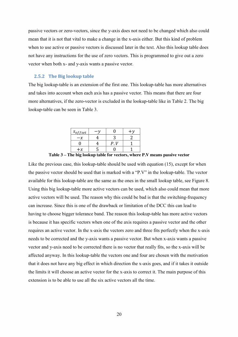
2.5.2 The Big lookup table

The big lookup-table is an extension of the first one. This lookup-table has more alternatives

and takes into account when each axis has a passive vector. This means that there are four

more alternatives, if the zero-vector is excluded in the lookup-table like in Table 2. The big

lookup-table can be seen in Table 3.

𝑠 −𝑦 0 +𝑦 −𝑥 4 3 2 0 4 𝑃. 𝑉 1 +𝑥 5 0 1

Table 3 – The big lookup table for vectors, where P.V means passive vector

Like the previous case, this lookup-table should be used with equation (15), except for when

the  passive  vector  should  be  used  that  is  marked  with  a  “P.V”  in  the  lookup-table. The vector

available for this lookup-table are the same as the ones in the small lookup table, see Figure 8.

Using this big lookup-table more active vectors can be used, which also could mean that more

active vectors will be used. The reason why this could be bad is that the switching-frequency

can increase. Since this is one of the drawback or limitation of the DCC this can lead to

having to choose bigger tolerance band. The reason this lookup-table has more active vectors

is because it has specific vectors when one of the axis requires a passive vector and the other

requires an active vector. In the x-axis the vectors zero and three fits perfectly when the x-axis

needs to be corrected and the y-axis wants a passive vector. But when x-axis wants a passive

vector and y-axis need to be corrected there is no vector that really fits, so the x-axis will be

affected anyway. In this lookup-table the vectors one and four are chosen with the motivation

that it does not have any big effect in which direction the x-axis goes, and if it takes it outside

the limits it will choose an active vector for the x-axis to correct it. The main purpose of this

extension is to be able to use all the six active vectors all the time.

21

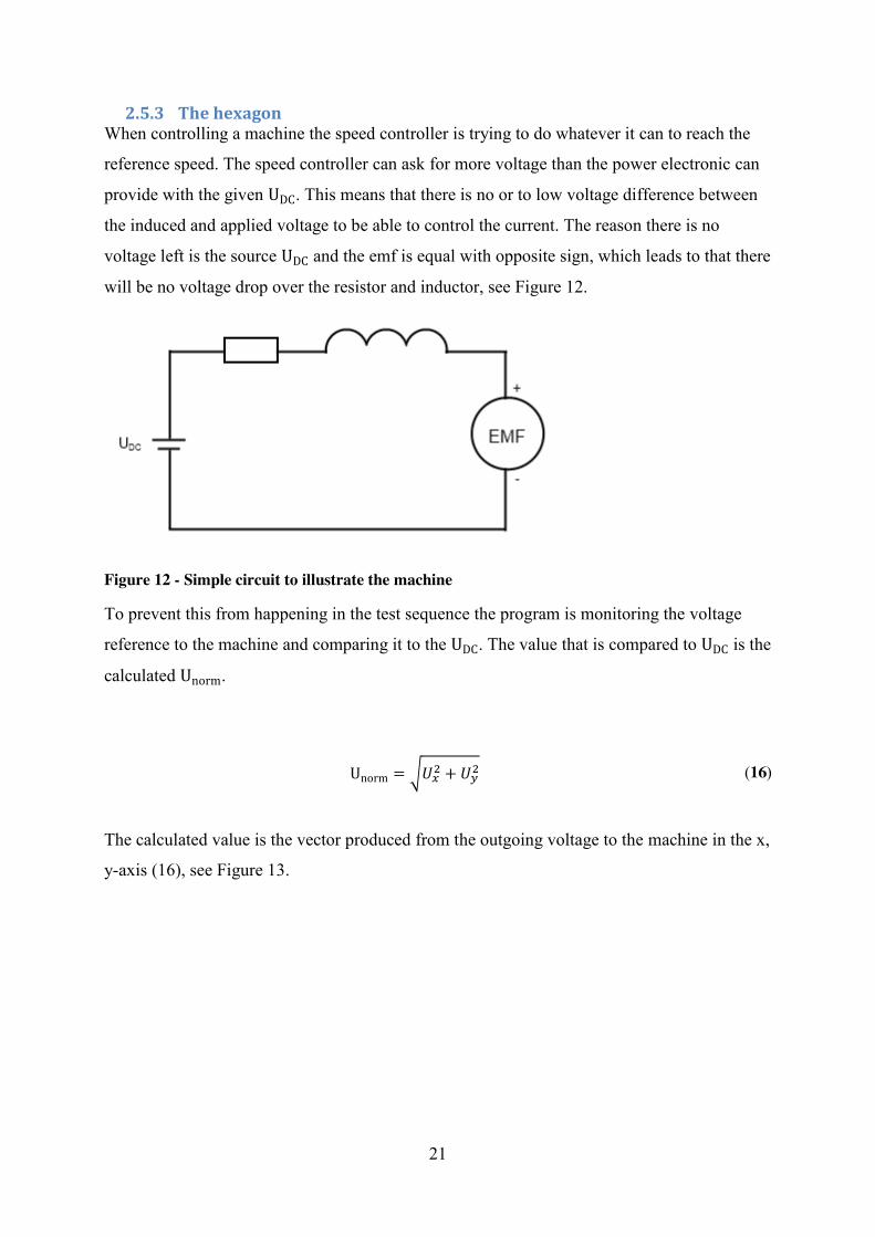
2.5.3 The hexagon When controlling a machine the speed controller is trying to do whatever it can to reach the

reference speed. The speed controller can ask for more voltage than the power electronic can

provide with the given UDC. This means that there is no or to low voltage difference between

the induced and applied voltage to be able to control the current. The reason there is no

voltage left is the source UDC and the emf is equal with opposite sign, which leads to that there

will be no voltage drop over the resistor and inductor, see Figure 12.

Figure 12 - Simple circuit to illustrate the machine

To prevent this from happening in the test sequence the program is monitoring the voltage

reference to the machine and comparing it to the UDC. The value that is compared to UDC is the

calculated Unorm.

The calculated value is the vector produced from the outgoing voltage to the machine in the x,

y-axis (16), see Figure 13.

Unorm = 𝑈 + 𝑈 (16)

22

Figure 13 - Hexagon for Unorm, the circle marks the limit for the voltage

The limitation in the test sequence is that when the ingoing voltage to the machine is 85% of

UDC the test should continue to the next step or point. This limit is not fixed, but in this test

sequences 15% of the voltage is saved to be able to change reference fast and aggressive.

23

2.5.4 Example for the DCC

Figure 14- Example of a dcc cycle

In Figure 14 there is an illustration of how the DCC works. For simplicity the example will be

in only one axis. That means that this example shows how §§ Table 1 works. This is an

example where there are three cases, two cases where the emf is bigger than zero and one

where the emf is less than zero. The difference between these cases is that for the ones where

the emf is bigger than zero the current decreases with passive vectors and vice versa. To

illustrate the changes they are marked with vertical dotted lines. The solid straight line making

a step is the reference value in this picture. And the rippling solid line is the actual current, the

dotted horizontal lines is the tolerance bands. The table below the picture is the value for each

of the x- and y-tolerance band circuit, see Figure 11. When the value is minus one it has

previously crossed the upper limit of the band, and if it is one it has previously crossed the

lower band. Since we have a controller with double tolerance band there are two limits. The

one closest to the reference value is called the "inner", and the bigger band is called the

"outer". Under this text the walkthrough of the picture will be made to understand the

principal of how the DCC actually works.

24

1. In the first rush on the way up to catch up the reference value the values of inner and

outer are not known for sure if the program has just started, but most likely it will be 1

on both inner and outer.

2. When it reaches the top band of the inner band, the value "inner" will be  1. Then it

starts moving down with the passive vector until it reaches the bottom band of “inner”

and the value inner will be changed to  −1.

3. Now the active vector is activated to push the current up. It will have an active value

until it reaches the top band of the inner band and again change "inner" to  1.

4. This will make the current fall with the passive vector. But before it reaches the

bottom limit of the inner band the emf changes, which means that the current is now

increasing with a passive vector.

5. Since it still has  1 as the value in "inner" it will continue to the upper band of the outer

band. When it reaches this band it will change the value "outer" to  1, and still the

value "inner" is unchanged.

6. This means that it has to decrease with an active vector and instead increase with a

passive vector. With "inner" = 1 and "outer" = 1" it will decrease with an active

vector until it reaches the lower inner band, see §§ Table 1.

7. When this happens the value "inner" is changed to  1. This makes the current increase

with a passive vector until it reaches the top band of the inner band.

25

This goes on in the picture in the same manners and one more change occurs in the emf. But

from the explanation so far one conclusion can be made. Depending on the values of "inner"

and "outer" the controller knows what it is supposed to do and that is done by using a lookup

table, see Table 2 and Table 3. Depending on these values the controller decides what action

is the most suitable. The lookup table is shown in §§ Table 1. Next to the lookup-table the

actions are also written. There are three actions that can be made, and those are to put zero,

+UDC or −UDC as an output voltage over the transistors. When zero is put in the output this is

called a passive vector and the other two are then called active vectors. An illustration of the

tolerance band is shown in Figure 15. A simplified picture of the tolerance band used in this

example can be seen in Figure 16, where the term rest is the use of passive vectors.

Figure 15 – How the tolerance band box looks like in x, y-frame, this has simple bands in the x frame

Figure 16 - Simplified Tolerance band used in this example [3, p. 103]

26

3 Implementation For the implementation of this Project National Instruments LabView and Matlab is used.

LabView is a graphical programming language that is used to implement the DCC. For the

DCC a FPGA module is used which offers parallel execution and via I/O modules the fast

sampling that is necessary for this implementation. To make the DCC work with the already

implemented test method some subVI was implemented to support it. The main programming

was made in the FPGA level, but some minor changes have also been made in the RT and PC

levels. All the implementation will be explained in this chapter but the code documentation

will be put in the Appendix A)

All the post-processing and calculation is done in Matlab. The measured data that is collected

from LabView will be processed in Matlab to get the results of the machine testing. The code

has also been modified to fit both the PI-controller and DCC.

3.1 DCC development A DCC that controls both the x- and y-currents is implemented. To make this possible, two

identical controllers with the same characteristics are developed. In both axes the tolerance

bands are identical which gives a box in the x, y-frame, see Figure 15. The DCC has both

inner and outer tolerance band so that passive vectors can be used.

Both lookup tables, the small and big-lookup table are implemented. They both use the

passive vectors when both x- and y-axis wants passive vectors. The difference between the

two lookup-tables is what vector to use when one axis requires a passive and the other

requires wants an active vector.

27

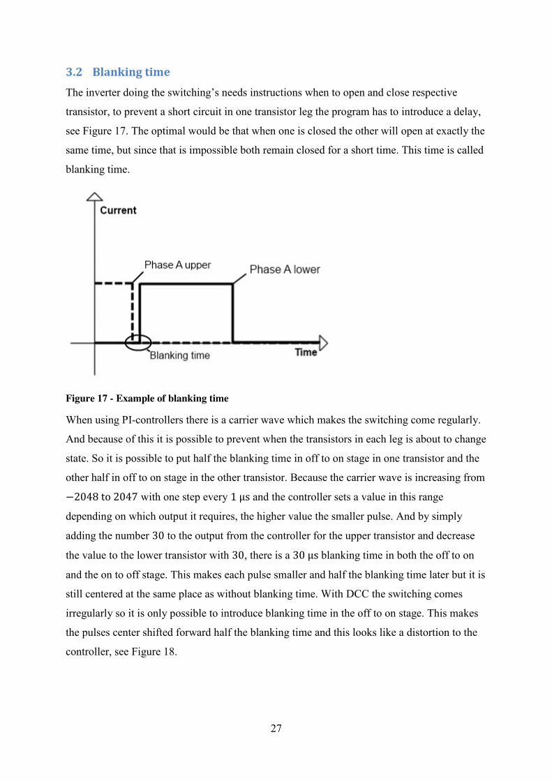
3.2 Blanking time The inverter doing the switching’s needs instructions when to open and close respective

transistor, to prevent a short circuit in one transistor leg the program has to introduce a delay,

see Figure 17. The optimal would be that when one is closed the other will open at exactly the

same time, but since that is impossible both remain closed for a short time. This time is called

blanking time.

Figure 17 - Example of blanking time

When using PI-controllers there is a carrier wave which makes the switching come regularly.

And because of this it is possible to prevent when the transistors in each leg is about to change

state. So it is possible to put half the blanking time in off to on stage in one transistor and the

other half in off to on stage in the other transistor. Because the carrier wave is increasing from

−2048  to  2047 with one step every 1  µμs and the controller sets a value in this range

depending on which output it requires, the higher value the smaller pulse. And by simply

adding the number 30 to the output from the controller for the upper transistor and decrease

the value to the lower transistor with 30, there is a 30  µμs blanking time in both the off to on

and the on to off stage. This makes each pulse smaller and half the blanking time later but it is

still centered at the same place as without blanking time. With DCC the switching comes

irregularly so it is only possible to introduce blanking time in the off to on stage. This makes

the pulses center shifted forward half the blanking time and this looks like a distortion to the

controller, see Figure 18.

28

Figure 18 - How the blanking time affect each pulse for both DCC and PI

3.3 FPGA DCC requires fast sampling and calculation to be able to control the machine. With earlier

equipment the sampling frequency was around 10 kHz which is too slow for a DCC, with

FPGA the sampling-frequency is 1 MHz. This makes it possible to implement a DCC for

controlling electric machines.

Figure 19 - The different parts of an FPGA [7]

FPGA is a reprogrammable silicon chip, see Figure 19, where new programming can be sent

to the chip via Ethernet-cable. The FPGA is fast because everything runs in parallel. This

means that the different tasks does not need to wait to execute, instead they run the task again

and again as fast as possible and sends the result to the outputs and indicators. To use this in

the most efficient way all the calculations and measurements should be done in the FPGA.

29

Every single operation takes 25 ns and is called a tick. Tick is a unit commonly used when

programming with FPGA just because one tick is one operation.

3.4 Switching Frequency When using a DCC a big drawback is that the switching frequency is variable. The switchings

can happen whenever the DCC wants. As long as it is low this is not a problem, except for the

fact that it is probably controlling the current badly. When the frequency is too high the

transistors can be damaged.

A way to reduce this problem is to make sure the DCC uses passive vectors often, this reduces

the switchings since a passive vector does not have the fast dynamics as an active vector. This

is the reason that there are two different lookup tables for the DCC. One that should use the

passive vectors more, which is the small lookup table, see Table 2. In the big lookup table

(Table 3) the focus is more to be able to use the vectors in a better way. If the x-axis needs to

be regulated but not the y-axis a vector that can do that should be used. This is of course not

always possible since there are only six different (active) vectors.

3.5 Implementation LabView consists of three major components, PC, RT and FPGA part, see Figure 20. They

have their strengths and drawbacks but put together the parts creates a strong unit. The

PC part uses the performance of the computer and is good for plotting and to save data to file.

The RT is used to control the FPGA and to process some data to PC part, there are limited

resources in the RT part and it is not as fast as the FPGA, so all calculation, regulation and

sampling is done in the FPGA. There are some improvement in the code on all three levels

from our side, but mainly in the FPGA, these improvements can be seen in this the appendix.

Figure 20 - The connection between the different levels

30

3.5.1 PC The  only  new  implementation  in  the  PC  is  the  plotting  of  the  “fast  fifo”.  The  fast  fifo  is  

plotted in separate plots. The two plots have their own update button and a delay controller for

the plots. With this the resolution of the plot can be set. The minimum delay possible is

1,25 µμs  (~50  ticks).

3.5.2 RT To make the dcc possible to control from the Real Time (RT) some controller need to be

available from the FPGA. Since the FPGA-code should not be controlled when doing the

testing, controlling the FPGA is supposed to be done from the RT. Therefore the only thing

that can be changed from the RT is the tolerance band. Also a controller is put to be able to

change between the DCC and the PI-controller. A feature that will not be used much, but can

be used for comparison is the button from double or simple tolerance band in the x-axis. The

reason that this option exist for the x- and not the y-axis is that the y-axis is more dynamic, it

changes more often, so a try to make the code simpler and if possible use less active vectors.

3.5.3 FPGA

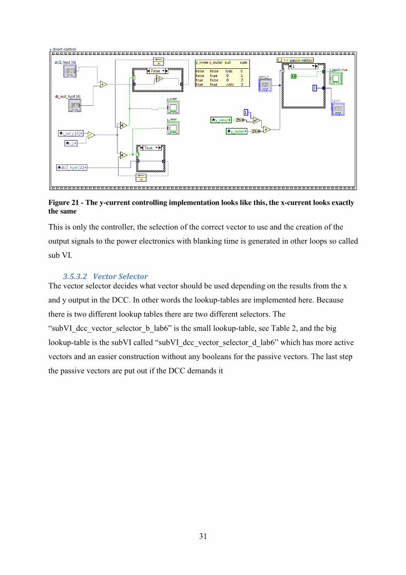
3.5.3.1 DCC The implemented block in the FPGA consists of two identical blocks, one for x and one for y

current, see Figure 21. To the left are the parameters, such as the tolerance band, the reference

and the actual current value. On the right there is the output, increase or decrease the current

and if it is ok to use passive vector. The small boxes in the middle are for shifting which limit

in the tolerance band to check against. If the current comes from negative we only check

against the positive one and vice versa.

The output from the comparison comes as true or false. True is equal to one and false is equal

to zero. The signals are added and go into a case loop with four cases, 0  to  3. Each case sets

the parameters to the output signals passive/active and increase/decrease. These output signals

is taken care of differently.

31

Figure 21 - The y-current controlling implementation looks like this, the x-current looks exactly the same

This is only the controller, the selection of the correct vector to use and the creation of the

output signals to the power electronics with blanking time is generated in other loops so called

sub VI.

3.5.3.2 Vector Selector The vector selector decides what vector should be used depending on the results from the x

and y output in the DCC. In other words the lookup-tables are implemented here. Because

there is two different lookup tables there are two different selectors. The

“subVI_dcc_vector_selector_b_lab6”  is  the  small lookup-table, see Table 2, and the big

lookup-table  is  the  subVI  called  “subVI_dcc_vector_selector_d_lab6”  which  has  more  active  

vectors and an easier construction without any booleans for the passive vectors. The last step

the passive vectors are put out if the DCC demands it

32

3.6 Hardware setup In this thesis the following equipment are used:

National Instruments CompactRIO-9022

o National Instruments Chassis c-RIO 9116

Module NI 9223

Module NI9215

Module NI9205

Module NI9263

Module NI9401

Module NI9402

Inverter: Semikron SKiiP 513 GB 172 CT

LEM current module LT 100-S

33

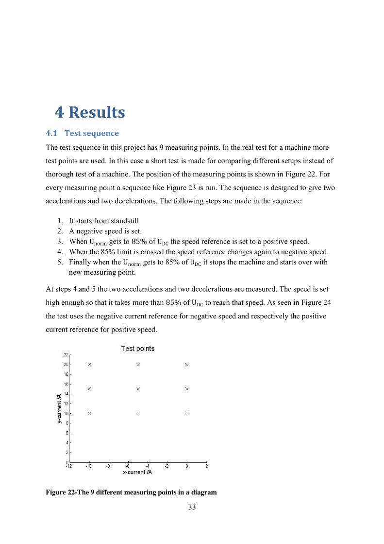
4 Results 4.1 Test sequence The test sequence in this project has 9 measuring points. In the real test for a machine more

test points are used. In this case a short test is made for comparing different setups instead of

thorough test of a machine. The position of the measuring points is shown in Figure 22. For

every measuring point a sequence like Figure 23 is run. The sequence is designed to give two

accelerations and two decelerations. The following steps are made in the sequence:

1. It starts from standstill 2. A negative speed is set. 3. When Unorm gets to 85% of UDC the speed reference is set to a positive speed. 4. When the 85% limit is crossed the speed reference changes again to negative speed. 5. Finally when the Unorm gets to 85% of UDC it stops the machine and starts over with

new measuring point.

At steps 4 and 5 the two accelerations and two decelerations are measured. The speed is set

high enough so that it takes more than 85% of UDC to reach that speed. As seen in Figure 24

the test uses the negative current reference for negative speed and respectively the positive

current reference for positive speed.

Figure 22-The 9 different measuring points in a diagram

34

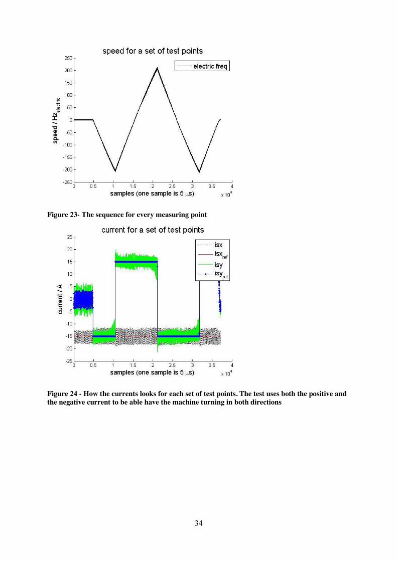
Figure 23- The sequence for every measuring point

Figure 24 - How the currents looks for each set of test points. The test uses both the positive and the negative current to be able have the machine turning in both directions

35

4.2 Small lookup table vs. Big lookup table To be able to compare the two lookup-tables some basic function will be compared. To get a

good comparison both tests will be under the same test-sequence with the same conditions.

The most important thing with the lookup-table is that the switching frequency can be

minimized without effecting controller’s characteristics in a bad way. Therefore the

comparison will be in the number of switching’s, which vectors are used (passive or active)

and how it performed in the test. Since a counter for the switching frequency is not

implemented the switching frequency is monitored from an oscilloscope to see that the limit is

not exceeded. For the test the tolerance band was set to 1,5 A for the inner and 1,5 A for the

outer.

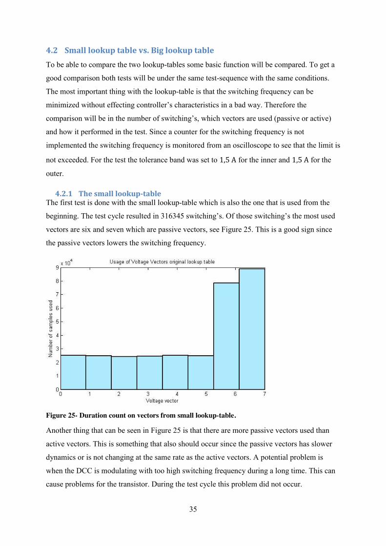
4.2.1 The small lookup-table The first test is done with the small lookup-table which is also the one that is used from the

beginning. The test cycle resulted in 316345 switching’s. Of those switching’s the most used

vectors are six and seven which are passive vectors, see Figure 25. This is a good sign since

the passive vectors lowers the switching frequency.

Figure 25- Duration count on vectors from small lookup-table.

Another thing that can be seen in Figure 25 is that there are more passive vectors used than

active vectors. This is something that also should occur since the passive vectors has slower

dynamics or is not changing at the same rate as the active vectors. A potential problem is

when the DCC is modulating with too high switching frequency during a long time. This can

cause problems for the transistor. During the test cycle this problem did not occur.

36

Figure 26 - The step response for the small lookup-table. The ripple is the current moving between the tolerance bands. The step is acceleration to deceleration

The most important thing for the lookup-table is to be able to control the current with as low

switching frequency as possible. In Figure 26 the step response is shown and from the graph

the current is following the reference well. The reason that the current is not exactly around

the reference is that there is not enough voltage to keep the current at -15 A. The lack of

voltage is because the speed of the machine is high and thus the big emf. When it changes the

reference it still has problem keeping the current around the reference but it is getting better

since the machine is now braking and the emf is getting smaller. When the step response

occurs it goes from acceleration to deceleration. Still the characteristics of a DCC can be seen

with the ripple and it is doing a good job keeping the current at an acceptable level close to

the reference value. Overall this lookup table is been good and has been used before. But if

there is a possibility to lower the switching frequency this would be better for the transistor

and in the need of better current control the tolerance band could be smaller.

37

4.2.2 The big lookup-table Like in the previous case the test cycle is the same so that a fair comparison can be done,

which means that the same DC-voltage, tolerance bands and the sequences is done after each

other. In the test cycle there were 312512 switching’s.

Figure 27 - Duration count on vectors from big lookup-table

During a test cycle mostly active vectors are used, see Figure 27. But still the most used

vectors is the passive vectors that were used ~70′000 times, while the active vectors are used

~30′000 times per vector. Even though less passive vectors are used the switching frequency

did not increase. This is a good sign which could mean that this lookup-table is more

effective. Also fewer switchings will be needed which helps reducing the switching

frequency.

38

Figure 28 - The step response for the big lookup-table and the current ripple is the current rippling between the tolerance bands. The step is acceleration to deceleration

The step response when using the big lookup-table can be seen in Figure 28. The current has

some problems following the current when the current is −15A, this is due to the back emf

from the machine that is running in a high speed. But when the current changes to 15 A the

current is oscillating around the reference as it should be. The ripple from the DCC can be

seen, but this time it is a bit smaller at the top. Like the previous case it goes from acceleration

to deceleration in the step response.

39

4.2.3 Comparison of the results The first thing that should be compared is how many switchings there were under the test

sequence. In this comparison the big lookup-table has fewer switchings. The difference was

3833 switchings. This is not a very big difference considering that during a testing cycle there

is about 300′000 switchings.

Another thing that differs is that more active vectors are used for the big lookup-table. But the

difference is small since every active vector is used maybe 1000  to  2000 samples more when

the total is around 30‘000 samples. This does not mean that there is more switching since it

could only mean that it stays longer on a specific vector, the passive vectors also differs. In

this case the small lookup-table uses about 15′000 more passive vectors. In the text it is said

that passive vectors are better because they bring down the switching frequency. But since the

switching frequency is about the same in both cases, this can mean that they have similar

characteristics.

Both are equally good when the step responses are compared. This is not that surprising since

the main task of these lookup tables is to reduce the switching frequency. Both behave the

same and give the same result in the test which indicates that the different lookup tables do

not affect the results of the test.

The difference between the big and the small lookup tables are very small and behave very

similar. The most noticeable difference is how the vectors are used. From the result it looks

like the big lookup-table uses the vectors more effectively since it has fewer switchings even

though it uses more active vectors and still manages to keep the switching frequency at the

same level as the small lookup-table.

4.3 DCC vs. PI The electric machine used for the testing is a PMSM and the rotor fitted is not cogging

optimized. This meaning there is a lot of cogging and this can be seen in the Figure 29 which

shows the electric frequency plotted against the theta. It can also be seen in the Figure 30 as

the sinus variation around the reference value.

40

Figure 29 - Electric frequency against continuous theta, the sinus variation is due to cogging

The amplitude of the sinus is in this case  3  A. In this specific sequence the reference values

where 10, 15, 20  A in y current and 0,−10,−15  A in x-current. Even if the variation is big

compared to the reference the mean value is the same as the reference value.

When using the DCC controller and putting the tolerance band closer to the reference than the

variation created by the cogging, the sinus variation is replaced by the current ripple coming

with the controller. In Figure 30 and Figure 31 the difference can be seen.

41

Figure 30 - The reference and the current is sinus shaped around the reference, this is with PI-controller

Figure 31 - The reference and the current around it, the inner tolerance band is set to 1 and the outer is set to 2

42

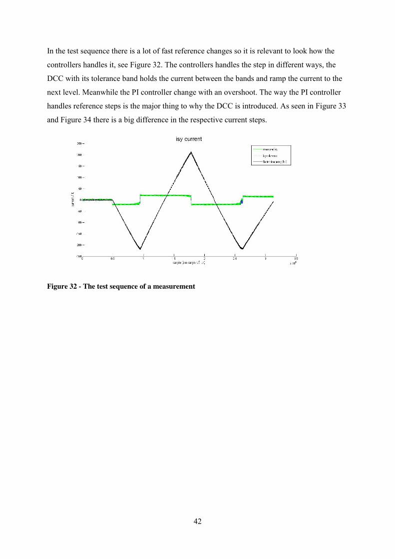
In the test sequence there is a lot of fast reference changes so it is relevant to look how the

controllers handles it, see Figure 32. The controllers handles the step in different ways, the

DCC with its tolerance band holds the current between the bands and ramp the current to the

next level. Meanwhile the PI controller change with an overshoot. The way the PI controller

handles reference steps is the major thing to why the DCC is introduced. As seen in Figure 33

and Figure 34 there is a big difference in the respective current steps.

Figure 32 - The test sequence of a measurement

43

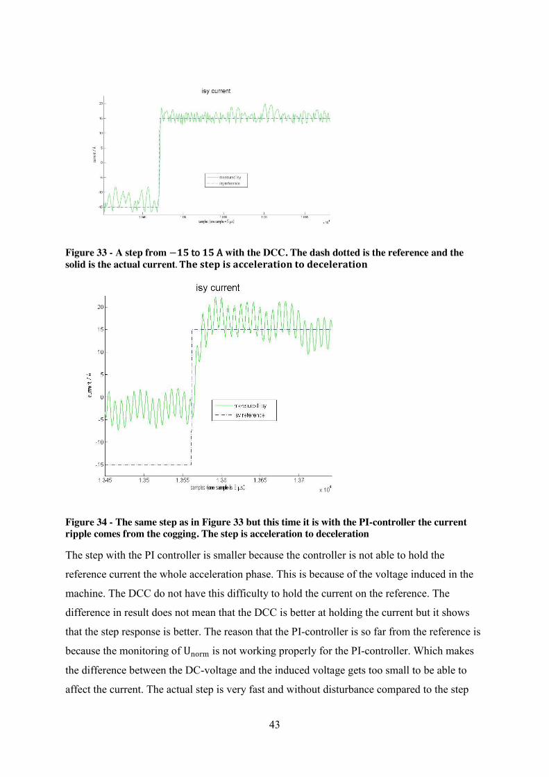
Figure 33 - A step from −𝟏𝟓  to  𝟏𝟓  A with the DCC. The dash dotted is the reference and the solid is the actual current. 𝐓𝐡𝐞  𝐬𝐭𝐞𝐩  𝐢𝐬  𝐚𝐜𝐜𝐞𝐥𝐞𝐫𝐚𝐭𝐢𝐨𝐧  𝐭𝐨  𝐝𝐞𝐜𝐞𝐥𝐞𝐫𝐚𝐭𝐢𝐨𝐧

Figure 34 - The same step as in Figure 33 but this time it is with the PI-controller the current ripple comes from the cogging. The step is acceleration to deceleration

The step with the PI controller is smaller because the controller is not able to hold the

reference current the whole acceleration phase. This is because of the voltage induced in the

machine. The DCC do not have this difficulty to hold the current on the reference. The

difference in result does not mean that the DCC is better at holding the current but it shows

that the step response is better. The reason that the PI-controller is so far from the reference is

because the monitoring of Unorm is not working properly for the PI-controller. Which makes

the difference between the DC-voltage and the induced voltage gets too small to be able to

affect the current. The actual step is very fast and without disturbance compared to the step

44

done with the PI-controller, it both takes much longer time and has an overshoot. It also takes

some time after the step before current reach its steady reference value. There is a superposed

sinus in the actual current that also can be derived from the cogging, this can also be seen in

the DCC case but it is not that apparent.

When plotting the x and y current against each other there will obviously be a quadrate in the

DCC case because that is how it is defined, but in the PI controller case it would theoretically

be a dot. But in reality it is a circle, and yet again it is the cogging creating this disturbance. In

the LabView program there is an x, y current plot and in Figure 35 and Figure 36 a screenshot

of this plot can be seen.

45

Figure 35 - A screenshot of the x, y-plot from the LabView program when using the DCC as controller. The box is the expected behavior of a DCC.

Figure 36 - A screenshot of the x, y-plot from the LabView interface then using the PI-controller. The expected result is a dot, but the cogging makes it a circle.

46

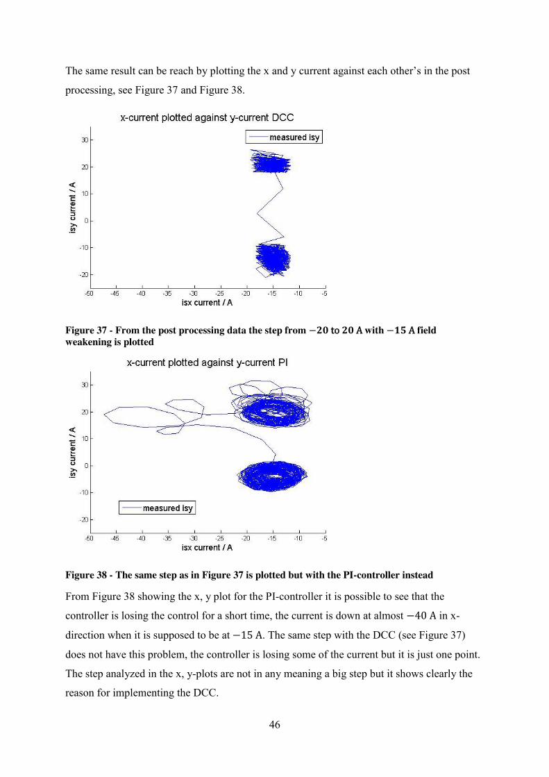
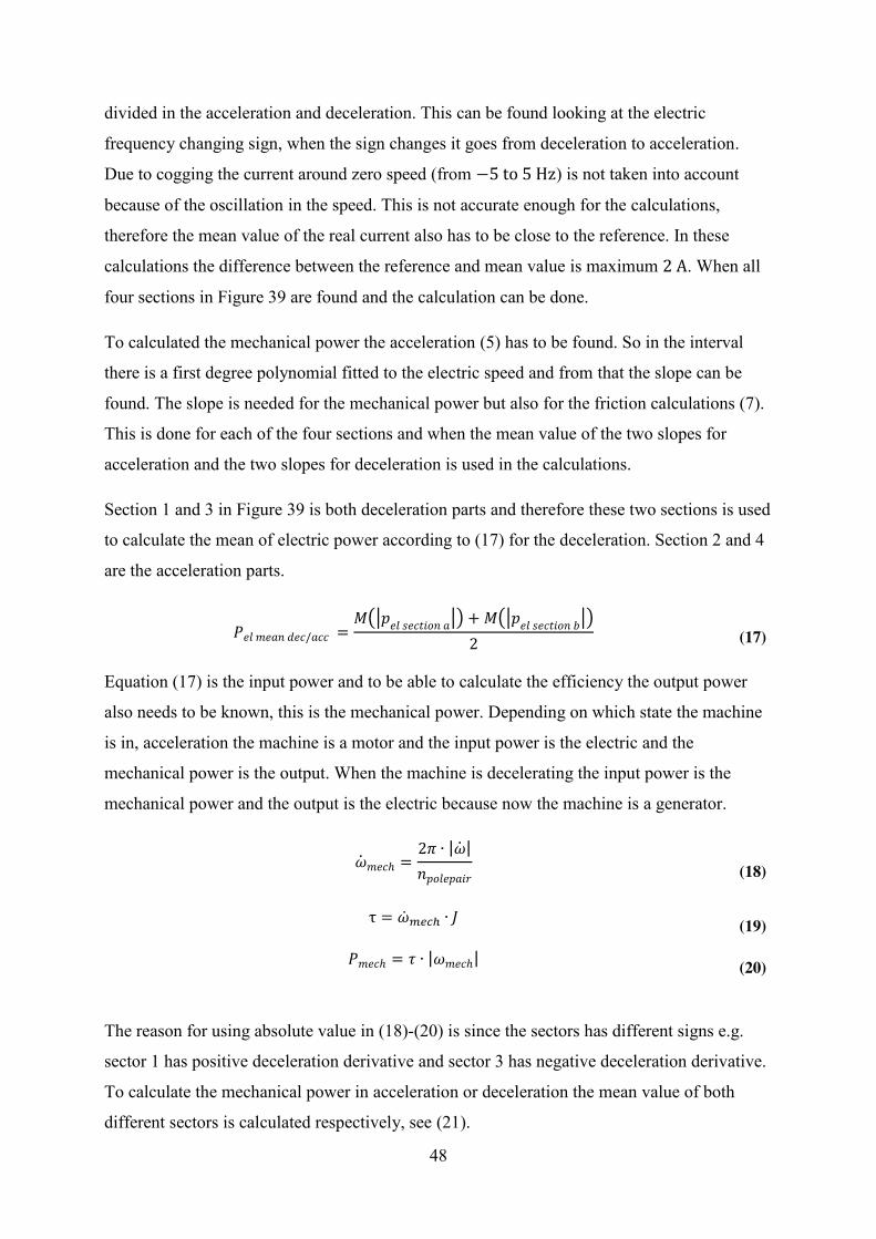
The  same  result  can  be  reach  by  plotting  the  x  and  y  current  against  each  other’s  in  the  post  

processing, see Figure 37 and Figure 38.

Figure 37 - From the post processing data the step from −𝟐𝟎  to  𝟐𝟎  A with −𝟏𝟓  A field weakening is plotted

Figure 38 - The same step as in Figure 37 is plotted but with the PI-controller instead

From Figure 38 showing the x, y plot for the PI-controller it is possible to see that the

controller is losing the control for a short time, the current is down at almost −40  A in x-

direction when it is supposed to be at  −15  A. The same step with the DCC (see Figure 37)

does not have this problem, the controller is losing some of the current but it is just one point.

The step analyzed in the x, y-plots are not in any meaning a big step but it shows clearly the

reason for implementing the DCC.

47

To calculate the smallest possible tolerance band without getting to high switching frequency

is to take the time it takes for the current to increase one ampere and adjust the tolerance band

after that. This time is dependent on the difference between the DC voltage and the induced

voltage, the bigger difference the faster the current will increase. With little over 130  V in DC

voltage and the machine standing still the rise time is 300  ticks/A which is equal to  7,5  µμs/A.

This is the worst case scenario and assuming that the current does not use any passive vectors.

To the user the biggest different between the two controlling types is undoubtedly the sound,

where the PI controller runs smooth and with clear tone the DCC sparks and sounds like

something is terribly wrong with the machine. Which type of noise is preferred depends on

the situation and location.

4.4 Post processing results Each time a test sequence is run there is data sampled and stored for later processing. Because

the machine test has to be fast, all the measurements are saved to a file and the processing is

done later. In the post processing it is possible to calculate the efficiency and the friction

losses of the machine. The calculation is done under the constant acceleration and

deceleration parts, see Figure 39. To get only the data from these parts the program is looking

at the reference value and the mean value of the current in y-direction. To minimize the

cogging oscillations the mean value is calculated over theta, e.g. mean value of each electric

revolution.

Figure 39 - The different parts of a test sequence used in post-processing

The start of the constant current reference is found checking the reference current and looking

for the change of the sign from minus to plus or vice versa. But this constant line has to be

48

divided in the acceleration and deceleration. This can be found looking at the electric

frequency changing sign, when the sign changes it goes from deceleration to acceleration.

Due to cogging the current around zero speed (from −5  to  5  Hz) is not taken into account

because of the oscillation in the speed. This is not accurate enough for the calculations,

therefore the mean value of the real current also has to be close to the reference. In these

calculations the difference between the reference and mean value is maximum 2  A. When all

four sections in Figure 39 are found and the calculation can be done.

To calculated the mechanical power the acceleration (5) has to be found. So in the interval

there is a first degree polynomial fitted to the electric speed and from that the slope can be

found. The slope is needed for the mechanical power but also for the friction calculations (7).

This is done for each of the four sections and when the mean value of the two slopes for

acceleration and the two slopes for deceleration is used in the calculations.

Section 1 and 3 in Figure 39 is both deceleration parts and therefore these two sections is used

to calculate the mean of electric power according to (17) for the deceleration. Section 2 and 4

are the acceleration parts.

𝑃𝑒𝑙  𝑚𝑒𝑎𝑛  𝑑𝑒𝑐/𝑎𝑐𝑐   =𝑀 𝑝𝑒𝑙  𝑠𝑒𝑐𝑡𝑖𝑜𝑛  𝑎 + 𝑀 𝑝𝑒𝑙  𝑠𝑒𝑐𝑡𝑖𝑜𝑛  𝑏

2

(17)

Equation (17) is the input power and to be able to calculate the efficiency the output power

also needs to be known, this is the mechanical power. Depending on which state the machine

is in, acceleration the machine is a motor and the input power is the electric and the

mechanical power is the output. When the machine is decelerating the input power is the

mechanical power and the output is the electric because now the machine is a generator.

�̇�𝑚𝑒𝑐ℎ =2𝜋 ∙ |�̇�|𝑛𝑝𝑜𝑙𝑒𝑝𝑎𝑖𝑟

(18)

τ = �̇� ∙ 𝐽

(19)

𝑃𝑚𝑒𝑐ℎ = 𝜏 ∙ |𝜔𝑚𝑒𝑐ℎ|

(20)

The reason for using absolute value in (18)-(20) is since the sectors has different signs e.g.

sector 1 has positive deceleration derivative and sector 3 has negative deceleration derivative.

To calculate the mechanical power in acceleration or deceleration the mean value of both

different sectors is calculated respectively, see (21).

49

𝑃𝑚𝑒𝑐ℎ  𝑚𝑒𝑎𝑛  𝑑𝑒𝑐/𝑎𝑐𝑐 =𝑀 𝑝𝑚𝑒𝑐ℎ  𝑠𝑒𝑐𝑡𝑖𝑜𝑛  𝑎 + 𝑀 𝑝𝑚𝑒𝑐ℎ  𝑠𝑒𝑐𝑡𝑖𝑜𝑛  𝑏

2

(21)

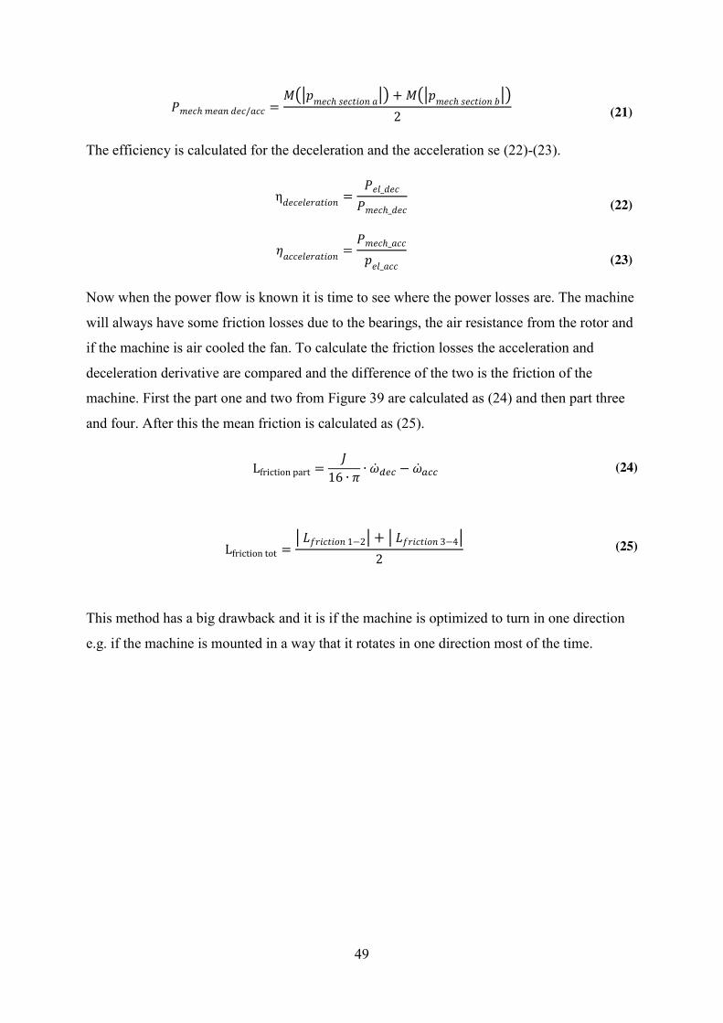
The efficiency is calculated for the deceleration and the acceleration se (22)-(23).

η𝑑𝑒𝑐𝑒𝑙𝑒𝑟𝑎𝑡𝑖𝑜𝑛 =𝑃𝑒𝑙_𝑑𝑒𝑐

𝑃𝑚𝑒𝑐ℎ_𝑑𝑒𝑐

(22)

𝜂𝑎𝑐𝑐𝑒𝑙𝑒𝑟𝑎𝑡𝑖𝑜𝑛 =𝑃𝑚𝑒𝑐ℎ_𝑎𝑐𝑐

𝑝𝑒𝑙_𝑎𝑐𝑐

(23)

Now when the power flow is known it is time to see where the power losses are. The machine

will always have some friction losses due to the bearings, the air resistance from the rotor and

if the machine is air cooled the fan. To calculate the friction losses the acceleration and

deceleration derivative are compared and the difference of the two is the friction of the

machine. First the part one and two from Figure 39 are calculated as (24) and then part three

and four. After this the mean friction is calculated as (25).

 Lfriction  part =𝐽

16 ∙ 𝜋 ∙ �̇� − �̇� (24)

Lfriction  tot =  𝐿𝑓𝑟𝑖𝑐𝑡𝑖𝑜𝑛  1−2 +  𝐿𝑓𝑟𝑖𝑐𝑡𝑖𝑜𝑛  3−4

2 (25)

This method has a big drawback and it is if the machine is optimized to turn in one direction

e.g. if the machine is mounted in a way that it rotates in one direction most of the time.

50

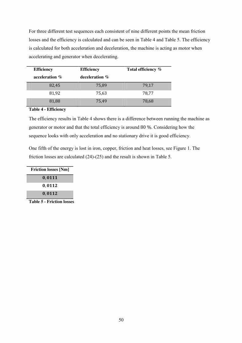
For three different test sequences each consistent of nine different points the mean friction

losses and the efficiency is calculated and can be seen in Table 4 and Table 5. The efficiency

is calculated for both acceleration and deceleration, the machine is acting as motor when

accelerating and generator when decelerating.

Efficiency acceleration %

Efficiency deceleration %

Total efficiency %

82,45 75,89 79,17

81,92 75,63 78,77

81,88 75,49 78,68

Table 4 - Efficiency

The efficiency results in Table 4 shows there is a difference between running the machine as

generator or motor and that the total efficiency is around  80  %. Considering how the

sequence looks with only acceleration and no stationary drive it is good efficiency.

One fifth of the energy is lost in iron, copper, friction and heat losses, see Figure 1. The

friction losses are calculated (24)-(25) and the result is shown in Table 5.

Friction losses [Nm]

𝟎, 𝟎𝟏𝟏𝟏

𝟎, 𝟎𝟏𝟏𝟐

𝟎, 𝟎𝟏𝟏𝟐

Table 5 - Friction losses

51

5 Conclusion and further development

5.1 Lookup-tables Both lookup-table had similar switching frequency and did not differ much. The small

lookup-table had more passive vectors and less active, but had more switchings during the

whole cycle. The big lookup-table had more active vectors and less passive and still managed

to have less switchings. This shows that the big lookup table is most likely more effective and

could maybe bring down the switching frequency but is still not significantly better. A good

thing is that the switching losses can be reduced during a longer cycle. In the test the

difference was around 1 % so the benefit would not be extremely good so far but will maybe

give better results on a longer sequence. To be sure which of the two is the better one a

counter for the switching frequency has to be implemented to detect the peaks in switching

frequency. Another thing is also how often it goes over the limit. These things have to be

closer investigated to get a definitive answer on which is the best choice. But since there is

less switching with the big lockup table it is our preferred choice.

5.2 DCC The simplicity of the DCC gives a lot advantages for this type of control with many reference

changes. The controller does not lose control over the current under the step as the PI-

controller does. This rotor used in the testing of the machine has cogging, and with DCC it is

not as visible in the current measurements anymore. Of course it is not completely gone, but

the clear sinus variation is not visible, it is in the noise of the DCC. On the speed

measurement the cogging is still visible. The DCC is doing a good job keeping the current

inside of the tolerance band, see Figure 35 and Figure 37, here is no sign of the circle the

cogging makes in the PI-controller see Figure 38.

52

A drawback of the DCC implemented in a setup with limited switching frequency, like ours,

is the non-constant switching frequency. But this can be taken care of by choosing tolerance

band wisely, meaning not choosing to small tolerance band according to the level of voltage

supply. The bigger supply the faster the current will rise. Choosing smaller tolerance band

will not always make the box smaller, e.g. if the band difference is smaller than the rise time.

The current will be outside the box when it is sampled and next time it is out on the other side,

this phenomenon will most likely result in too high switching frequency, if it is limited or to

slow sampling.

As mentioned before the noise of the DCC is not as clear as the tone from the PI controllers

fixed switch frequency. This irregularity in the sound can in some situation be found

annoying, but in a situation with much noise the sound of the DCC can disappear in the

background noise.

The DCC is a good replacement for the PI-controller. It keeps the current closer to the

reference and the step response is faster. The DCC can be even better at holding the current

closer to the reference. So far both the DCC and the PI is doing the job as current controller

well but the big question is witch has the biggest potential for further development.

5.3 Further developments As mentioned before in the chapter a counter for switching frequency has to be implemented,

one reason is deciding which of the look-up tables to choose from. Another reason is to be

able to better monitor the frequency momentarily during a test drive.

The big lookup-table could be further developed, especially when the y-axis is active and the

x-axis is passive, see Table 3.

In the DCC there is more room for development. The aim is to better follow the current, or

maybe have the current closer to the reference current. This is not only software based

problem but also the transistors would have to be able to handle higher switching frequency.

When to choose the active vectors can be optimized not only by the lookup-tables but also in

the DCC with inner and outer tolerance band. Since the x and y-axis are controlled

simultaneously there are some situations that are problematic to know for sure what is the best

thing to do? E.g. one calling for passive-, the other for active vector and the current is inside

the box, as it is implemented now it will choose an active vector.

53

The monitoring of Unorm is now working properly for the DCC but for the PI-controller it

stops the sequence too late so the difference between the DC-voltage and induced voltage gets

too small to affect the current. A temporary solution is that the limit is little bit lower for the

PI-controller than for the DCC.

54

6 References

[1] Energimyndigheten, "Energiläget 2011," Statens Energimyndighet, Eskilstuna, 2011.

[2] N. Urasaki, T. Senjyu and K. Ueza, "Influence of All Losses on Permanent Magnet

Synchronous Motor Drives," Department of Electrical and Electronic Engineering,

University of the Ryukyus, Senbaru Nishihara-cho Nakagami Okinawa 903-0213, Japan.

[3] P. Karlsson and M. Alaküla, Power Electronics Devices, Converters, Control and

Application.

[4] Y. Loayza, A. Reinap and M. Alaküla, "Performance and efficiency evaluation of FPGA

controlled IPMSM under dynamic loading," IEA at Lunds Tekniska Högskola, Lund.

[5] E. P. S. Caton, "Dynamic Braking, A new approach for testing Electrical Machines," Lund

Tekinska Högskola, Lund, 2011.

[6] D. M. Ingram and S. D. Round, "A Fully Digital Hysteresis Current Controller for an

Active Power Filter," Department of Electrical & Electronic Engineering, Christchurch,

New Zealand.

[7] "http://www.ni.com/white-paper/6983/en," National Instruments, 13 June 2012. [Online].

[8] D. M. I. a. S. D. Round, "A Fully Digital Hysteresis Current Controller for an Active

Power Filter," Department of Electrical & Electronic Engineering, Christchurch, New

Zealand.

[9] T. S. a. K. U. Naomitsu Urasaki, "Influence of All Losses on Permanent Magnet

Synchronous Motor Drives," Department of Electrical and Electronic Engineering,

University of the Ryukyus, Senbaru Nishihara-cho Nakagami Okinawa 903-0213, Japan.

55

7 Appendix

Table of Appendix APPENDIX A) CODE DOCUMENTATION OF THE DCC ................................................................................... 3

A.1 DCC DUTY OUT ........................................................................................................................................ 3

A.2 FAST FIFO ............................................................................................................................................... 3

A.3 FIFO ...................................................................................................................................................... 4

A.4 U_ABC2XY ............................................................................................................................................... 5

A.5 OUTPUT .................................................................................................................................................. 5

A.6 DCC ....................................................................................................................................................... 6

A.7 DCC VECTOR SELECTOR .............................................................................................................................. 7

A.8 CHANGES IN THE RT .................................................................................................................................. 8

A.9 CHANGES IN PC ........................................................................................................................................ 9

APPENDIX B) MATLAB CODE .................................................................................................................... 10

Table of Appendix figures FIGURE APPENDIX 1 – BLANKING TIME ............................................................................................................................. 3

FIGURE APPENDIX 2 – IMPLEMENTATION OF FAST FIFO....................................................................................................... 3

FIGURE APPENDIX 3 – FILTER OF UNORM ......................................................................................................................... 5

FIGURE APPENDIX 4 - DCC OR PI CONTROLLER SWITCH ....................................................................................................... 6

FIGURE APPENDIX 5 - IMPLEMENTATION OF THE DCC ......................................................................................................... 6

FIGURE APPENDIX 6 - VECTOR SELECTOR FOR THE SMALL LOOKUP-TABLE ................................................................................ 7

FIGURE APPENDIX 7 - VECTOR SELECTOR FOR THE BIG LOOKUP-TABLE .................................................................................... 7

FIGURE APPENDIX 8 - NEW IMPLEMENTATION IN RT ........................................................................................................... 8

FIGURE APPENDIX 9 - THE IMPLEMENTATION OF THE FAST FIFO IN PC ................................................................................... 9

2

Table of Appendix Tables TABLE APPENDIX 1 – VALUES IN THE FAST FIFO ................................................................................................................. 4

TABLE APPENDIX 2 – CHANGES MADE IN THE FIFO ............................................................................................................ 4

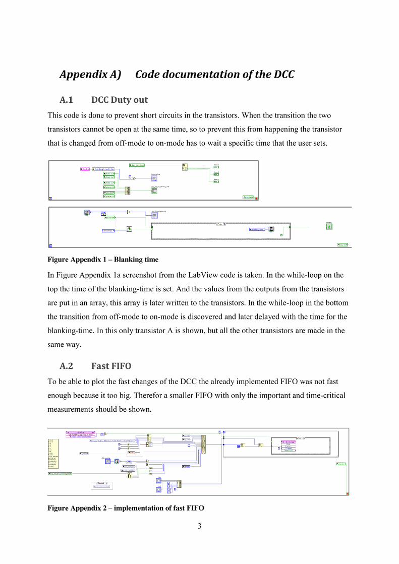
3

Appendix A) Code documentation of the DCC

A.1 DCC Duty out This code is done to prevent short circuits in the transistors. When the transition the two

transistors cannot be open at the same time, so to prevent this from happening the transistor

that is changed from off-mode to on-mode has to wait a specific time that the user sets.

Figure Appendix 1 – Blanking time

In Figure Appendix 1a screenshot from the LabView code is taken. In the while-loop on the

top the time of the blanking-time is set. And the values from the outputs from the transistors

are put in an array, this array is later written to the transistors. In the while-loop in the bottom

the transition from off-mode to on-mode is discovered and later delayed with the time for the

blanking-time. In this only transistor A is shown, but all the other transistors are made in the

same way.

A.2 Fast FIFO To be able to plot the fast changes of the DCC the already implemented FIFO was not fast

enough because it too big. Therefor a smaller FIFO with only the important and time-critical

measurements should be shown.

Figure Appendix 2 – implementation of fast FIFO

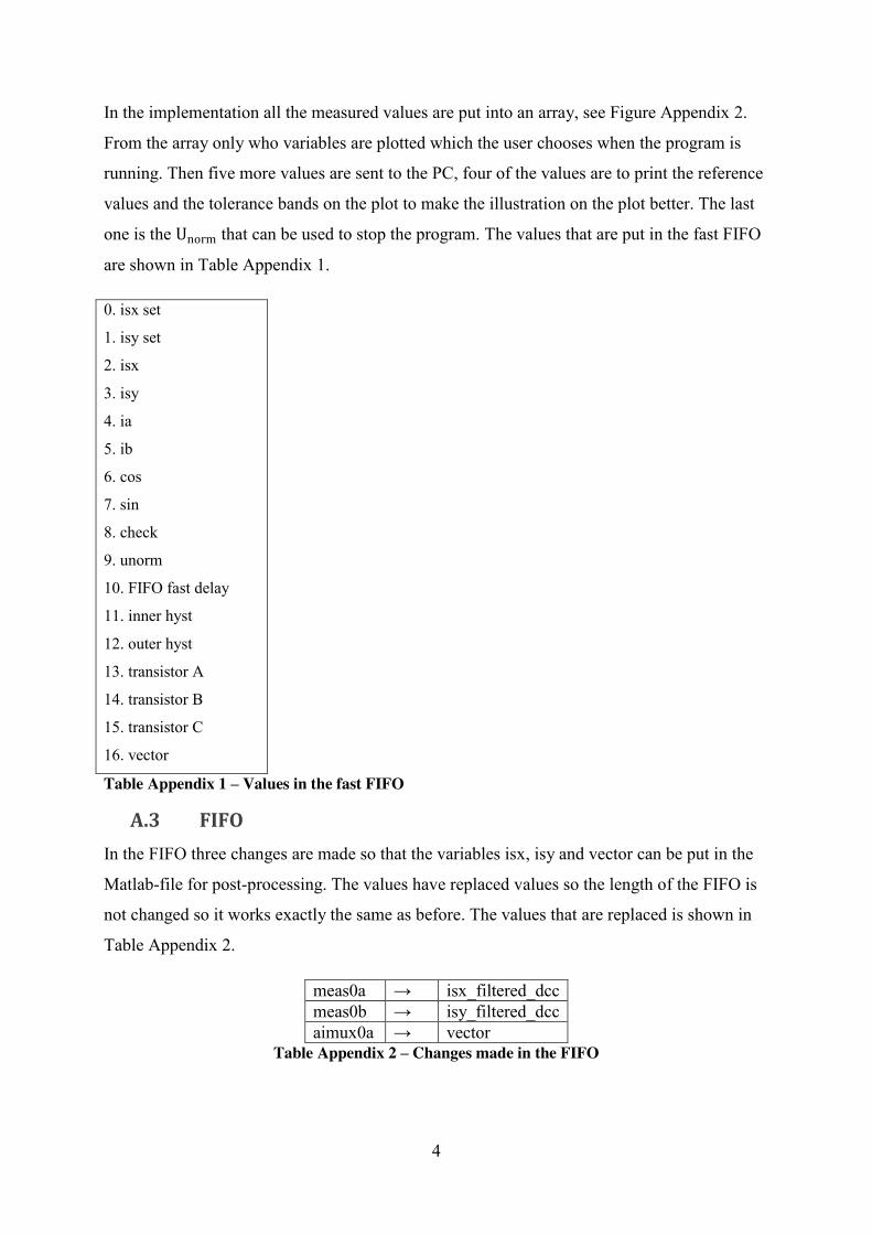
4

In the implementation all the measured values are put into an array, see Figure Appendix 2.

From the array only who variables are plotted which the user chooses when the program is

running. Then five more values are sent to the PC, four of the values are to print the reference

values and the tolerance bands on the plot to make the illustration on the plot better. The last

one is the Unorm that can be used to stop the program. The values that are put in the fast FIFO

are shown in Table Appendix 1.

0. isx set

1. isy set

2. isx

3. isy

4. ia

5. ib

6. cos

7. sin

8. check

9. unorm

10. FIFO fast delay

11. inner hyst

12. outer hyst

13. transistor A

14. transistor B

15. transistor C

16. vector

Table Appendix 1 – Values in the fast FIFO

A.3 FIFO In the FIFO three changes are made so that the variables isx, isy and vector can be put in the

Matlab-file for post-processing. The values have replaced values so the length of the FIFO is

not changed so it works exactly the same as before. The values that are replaced is shown in

Table Appendix 2.

meas0a → isx_filtered_dcc meas0b → isy_filtered_dcc aimux0a → vector

Table Appendix 2 – Changes made in the FIFO

5

A.4 u_abc2xy After implementing the DCC the value Unorm has become more important to monitor to make

sure that not too much voltage is taken out from the power electronics. That is why an

indicator is put out and the value is filtered so that a more stable value can be shown in the

PC.

Figure Appendix 3 – filter of Unorm

In Figure Appendix 3 the implementation of the filter is shown. In the u_norm_exp the value

of the filter is put. The value u_norm_filtered is sent to the PC-part to be read by the voltage

limiter.

A.5 Output In  the  loop  “Pulse  Width  modulation”  the  switch  between  DCC  and  PI  is  put.  Since  both  

controllers run in parallel the only thing to change is which of the output arrays to choose

from. The implementation of the switch is shown in Figure Appendix 4.

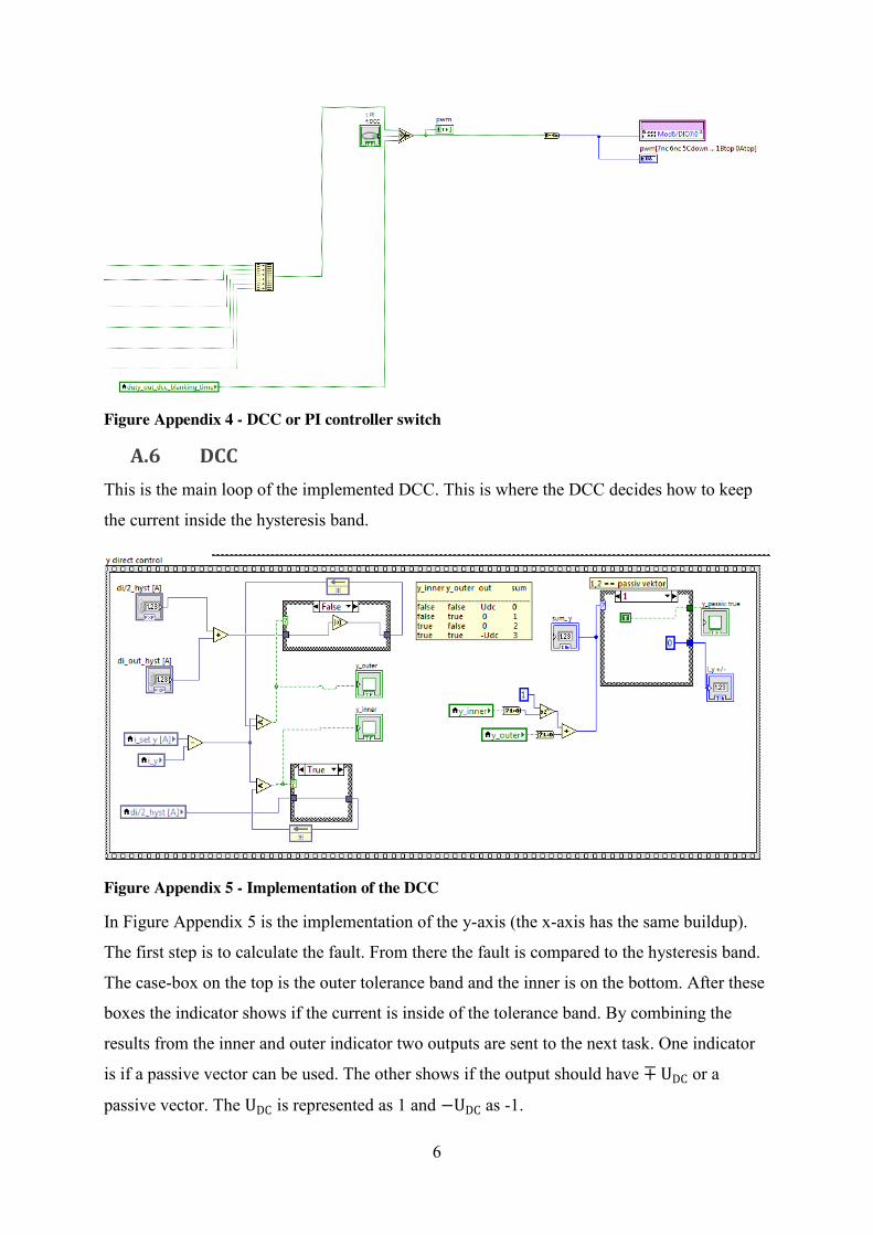
6

Figure Appendix 4 - DCC or PI controller switch

A.6 DCC This is the main loop of the implemented DCC. This is where the DCC decides how to keep

the current inside the hysteresis band.

Figure Appendix 5 - Implementation of the DCC

In Figure Appendix 5 is the implementation of the y-axis (the x-axis has the same buildup).

The first step is to calculate the fault. From there the fault is compared to the hysteresis band.

The case-box on the top is the outer tolerance band and the inner is on the bottom. After these

boxes the indicator shows if the current is inside of the tolerance band. By combining the

results from the inner and outer indicator two outputs are sent to the next task. One indicator

is if a passive vector can be used. The other shows if the output should have ∓  UDC or a

passive vector. The UDC is represented as 1 and −UDC as -1.

7

A.7 DCC vector selector At this point the right vector has to be used to get out the right output. This is done by taking

the result from the main DCC block and taking out the result from the lookup-table. Since

there are two different lookup-tables in this project there are two different implementations.

Both have similarities and are basically built up the same way but they look a little different.

Figure Appendix 6 - Vector selector for the small lookup-table

The small lookup-table (Figure Appendix 6) uses the result from the DCC of x, y-axis. To

know the position of the rotor the theta is also taken into account. The last thing that has to be

taken from the outside is the indicators for passive vectors.

In the first case-box the output is the offset that should be added to the sector that the rotor is

currently in. Since the result from the addition of the sector and offset can be overshoot this is

corrected in the middle case-box. In the last case-box the use of the passive vectors are set. To

use the passive vectors one of the x, y –axis has to be passive and the other has to be inside of

the outer tolerance band.

Figure Appendix 7 - Vector selector for the big lookup-table

In Figure Appendix 7 is the implementation of the big lookup-table. Like in the

implementation above the results from the DCC is taken. But in this case the result is

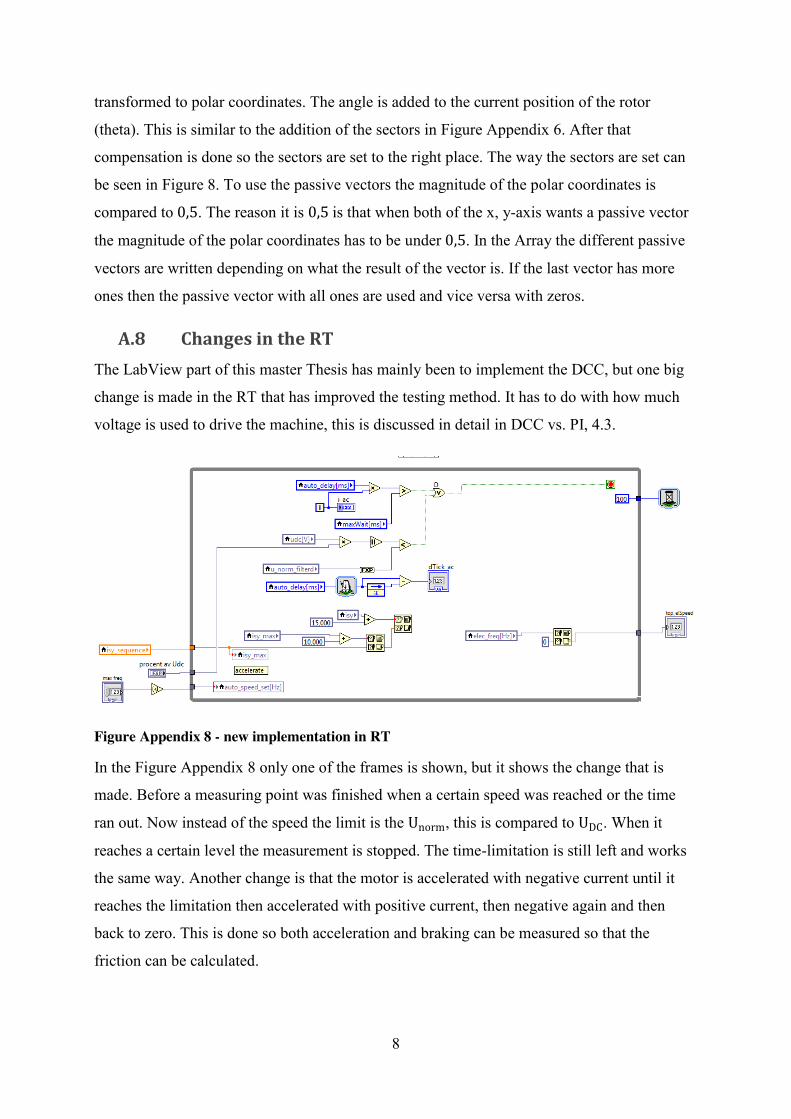
8

transformed to polar coordinates. The angle is added to the current position of the rotor

(theta). This is similar to the addition of the sectors in Figure Appendix 6. After that

compensation is done so the sectors are set to the right place. The way the sectors are set can

be seen in Figure 8. To use the passive vectors the magnitude of the polar coordinates is

compared to  0,5. The reason it is 0,5  is that when both of the x, y-axis wants a passive vector

the magnitude of the polar coordinates has to be under  0,5. In the Array the different passive

vectors are written depending on what the result of the vector is. If the last vector has more

ones then the passive vector with all ones are used and vice versa with zeros.

A.8 Changes in the RT The LabView part of this master Thesis has mainly been to implement the DCC, but one big

change is made in the RT that has improved the testing method. It has to do with how much

voltage is used to drive the machine, this is discussed in detail in DCC vs. PI, 4.3.

Figure Appendix 8 - new implementation in RT

In the Figure Appendix 8 only one of the frames is shown, but it shows the change that is

made. Before a measuring point was finished when a certain speed was reached or the time

ran out. Now instead of the speed the limit is the Unorm, this is compared to UDC. When it

reaches a certain level the measurement is stopped. The time-limitation is still left and works

the same way. Another change is that the motor is accelerated with negative current until it

reaches the limitation then accelerated with positive current, then negative again and then

back to zero. This is done so both acceleration and braking can be measured so that the

friction can be calculated.

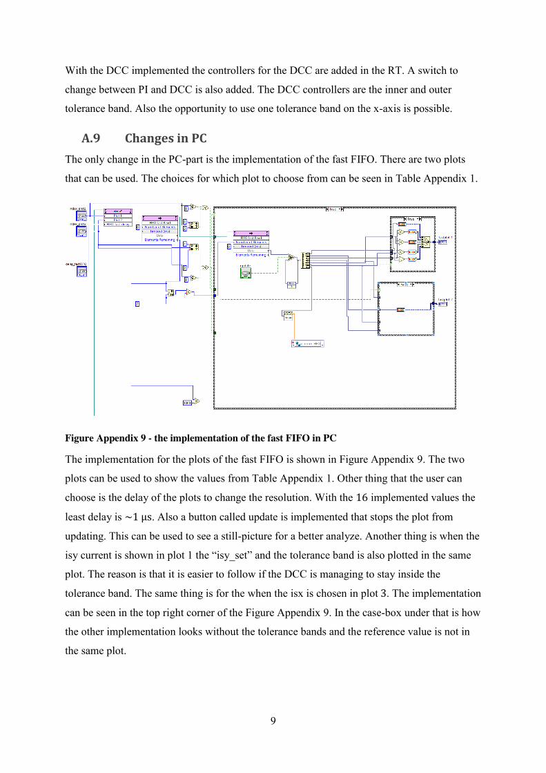
9

With the DCC implemented the controllers for the DCC are added in the RT. A switch to

change between PI and DCC is also added. The DCC controllers are the inner and outer

tolerance band. Also the opportunity to use one tolerance band on the x-axis is possible.

A.9 Changes in PC The only change in the PC-part is the implementation of the fast FIFO. There are two plots

that can be used. The choices for which plot to choose from can be seen in Table Appendix 1.

Figure Appendix 9 - the implementation of the fast FIFO in PC

The implementation for the plots of the fast FIFO is shown in Figure Appendix 9. The two

plots can be used to show the values from Table Appendix 1. Other thing that the user can

choose is the delay of the plots to change the resolution. With the 16 implemented values the

least delay is ~1  µμs. Also a button called update is implemented that stops the plot from

updating. This can be used to see a still-picture for a better analyze. Another thing is when the

isy  current  is  shown  in  plot  1  the  “isy_set”  and  the  tolerance  band  is  also  plotted  in  the  same  

plot. The reason is that it is easier to follow if the DCC is managing to stay inside the

tolerance band. The same thing is for the when the isx is chosen in plot  3. The implementation

can be seen in the top right corner of the Figure Appendix 9. In the case-box under that is how

the other implementation looks without the tolerance bands and the reference value is not in

the same plot.

10

Appendix B) Matlab code The source to our Matlab code is the file that Yury Loayza used for postprocessing his data.

This file has then been modified to fit also with the data generated then using a DCC. Since

the sequence is changed most of the code is rewritten to fit this. Also some additional

calculations are implemented, such as friction losses which comes from the difference in input

and output power from the electric machine. More about this is in the text. The filed use is

called “m20120516_powerCalculationLongSeq.m”. This file can be found at IEA, LTH.

There has also been some smaller files generated for comparison between the different

controllers and so on, this files is called “m20120523differentDCC_comp.m”.