ELECTRICAL STIMULATION OF LIMBSPART ID® JOINT POSITION CONTROL'

Alain Fournier

Laboratoire d'Automatique de MontpellierUniversite de Sciences et Techniques du LanguedocPlace E . Bataillon, 34060 Montpellier-Cedex, France

Etienne Dombre

I .N .S .E .R .M . U 103 Unite de Recherches BiomecaniquesAvenue des Moulins, 34000 Montpellier, France

Philippe CoiffetLaboratoire d'Automatique de Montpellier

Univesite de Sciences et Techniques du LanguedocPlace E . Bataillon, 34060 Montpellier-Cedex, France

INTRODUCTION

The physiological study of muscular contraction enables one to describethe mechanisms of nerve conduction (1), of synaptic transmission, ofamplification performed by the motor end-plates (2), and of contraction ofthe motor-units (3) . None of these descriptions enables one to obtain themathematical relationships which represent the total behavior of theneuromuscular loop . In order to obtain a simple model, we chose anelectromechanical representation of the process rather than a combina-tion of the models developed from the study of the structure and the char-acteristics of each element.

This paper describes the modeling and the position-control of a single-degree-of-freedom joint by means of pulse-width modulation of the signalsent to the agonist muscle 's nerve . The first part presents an experi-mental procedure devised from the previous results of this study (4,5) . Inthe second part, the mathematical methods used in order to identify theprocess and to analyze the results obtained are concisely shown.

aBased on work performed under VA Contract V101 (134) P-132 .

5

DYNAMIC STUDY OF A JOINT WITHA SINGLE DEGREE OF FREEDOM

Description of the Process

Measurements have been performed on ankles of anesthetized dogs.The tibia is maintained in a fixed horizontal position, and hence the pawrevolves in a vertical plane around an axis fixed in space . Electrical stim-ulation of the external popliteal sciatic nerve produces contraction of theanterior tihialis, and thus dorsiflexes the paw . The forces involved duringthe contraction period are:

1. The muscular force developed during the contraction of the agonist

muscle group;2. The muscular force coming from the stretched antagonist muscle

group which is not stimulated;3. The passive effects of ligaments and mechanical limits of the joint;4. The viscous damping forces, proportional to the rotational velocity;

and,5. The external load and the weight of the paw .

Pulley

FIGURE I . -- Diagram of an ankle joint.

In order to write the equations of the dynamic system, let us consider aschematic diagram of an ankle joint (Fig . 1) . b

bThe diagram given in Part II, Figure 22, p . 286, BPR 1022, is slightly different . For dogs, cand d are very small in comparison with the distances D I and D2 shown in Figure 22, i .e .,fO)2<1 . Thus, F l and F2 may be assumed to be parallel to the longitudinal axis of thetibia with negligible error.

6

Fournier et al . : Electrical Stimulation—Part III

siaOmmg L cos9 E dodt

where 9, F l and F 2 are the variables governing the motion ; j, c, d, M, m,

h, L, and are biomechanical parameters ; the physical parameters are jthe moment of inertia, m the mass of the paw and of the positiontransducer together, and the viscous damping coefficient.

Determination of the Biomechanical parameters

Equation [1] shows physical terms which are not easy to measure andwhich we were unable to compute with sufficient accuracy.

Measurement of j is difficult . The "quick release" method (6) can be

performed . Recording the period of oscillations of the free lever is anothermethod of computing the moment of inertia (7, 8) . Since thesemeasurements need complex experiments for each subject, we chose todivide equation [1] by the moment of inertia j and to express the para-meters as functions of the moment of inertia . Equation [I then becomes:

gh- sinO—mgL cosO i,dO

[2]

J

.f dt

The coefficients c and d represent the distances between the center ofrotation of the joint and the points where the forces developed by theagonist muscle group and antagonist muscle group, respectively, areapplied. We tried to determine these distances by dissection of a dog'sleg but accurate measurement was impossible because the tendonbranches, and its area of insertion on the bone is wide, thus making thecenter of pressure difficult to define . The mass M of the external load isknown with accuracy . However, the distance h between the center ofrotation of the joint and the point of application of the wire transmittingthe external force is inaccurate . The Mass m, of the paw and the positiontransducer together, and the distance L between the center of gravity ofthe paw and the joint center, cannot be measured directly . Computationof the viscous damping coefficent from the decrease in the paw oscilla-tions does not yield accurate results.

Among the variables governing the motion of the paw, only the jointangle can be directly measured during the experiment . It is very difficultto measure the force developed by the stimulated muscle and the passive

The equation is:

&8

dz 8dt'

effects of the system without measurably altering the system,' It is thusnecessary to proceed to other experiments in order to determine the

unknown forces.

Determination of the Control Signal and of the Joint Position

The conditions of this experiment are shown in Figure 2.

FIGURE 2 . -Experimental procedure.

The stimulator delivers pulses with a fixed frequency and amplitude of451-Iz and 150mV respectively ; control is achieved by pulse width

modulation from 10gs to 4ms) of the stimulation signal . This signal isrecorded as well as the joint position 9 (Fig . 3).

FIGURE 3 . —Recordings of the input signal (pulse width() and of the output signal (angular

position 0) (BECKMAN DYNOGRAPH R .M,).

c The method of measuring the force developed by the stimulated muscle by implantingtransducers in the muscle tendons as described in Part I, pp . 266-267, BPR 10-22, was aban-doned because of the following difficulties encountered : I . damage of tendons, 2 . continual

drift of output signals, and 3 . malfunction of the fragile transducers.

8

Fournier et al . : Electrical Stimulation—Part lif

The damped oscillations of 9, which are observed when the stimulationcauses overshoot (corresponding with the return of the external load to itsinitial position) are due, at least in part, to the mechanical vibrations ofthe metallic frame designed to maintain the tibia in a stable and

horizontal position . Tests have been performed with different external

loads; the pulse-width of the stimulation signal has been adjusted in orderto obtain the maximum rotation of the paw (about 30 deg).

Determination of the Antagonists' Passive Effects

Whereas the driving force depends on the stimulation signal, theantagonist forces are a function of the joint position only.

To determine the antagonists' resultant passive force FANT, the paw ismanually rotated through its full range of motion from one mechanical

Pulley RESTLENGTH

DYNAMETRICTRANSDUCER

FIGURE 4 . --Determination of the antagonists' effects .

MANUALTRACTION

limit of the joint to the other . Figure 4 shows the principle of the twoexperiments, 9 being the axis of rotation . We have:

Moment of FANToment of force

om manual tractio (Moment of mg) — (Moment of Mg)

The traction force on the dynamometer ring and the total angle of rotation are simultaneously recorded, The resulting curve, shown in Figure 5,is obtained after compensation for the gravity forces and allows one todetermine the antagonists' effects as a function of the joint position O.

U0

I 'l-°

Passive Stretch Passive Stretch

IF;Triceps Suree

oi4, 1

o Tibialis Anterior caa) to

4, I<vi

a

112,or

140ISO

160

FIGURE 5 . — Passive effects of P ANT as a function of ().

10

Fournier et al . : Electrical Stimulation—Part 111

Determination of the Muscular Force

Any surgical operation on the tendon changes its characteristics . In anattempt to avoid any alteration of the neuromuscular system, we decidedto wait until after the conclusion of the joint-position control experimentand then cut the tendon of the agonist muscle group . The experimentalprocedure followed is shown in Figure 6.

Fixation of tibia(by means of pins)

FIGURE 6 .-Experimental procedure,

A dynamometer ring is set along the main axis of the muscle. Underidentical stimulation conditions as in the first experiment, the isometricforce developed by the stimulated muscle is recorded (Fig . 7) . Therelationship between the stimulation signal and the muscular force whichis developed can then be characterized.

F(N)

0

0 .1

0 .2

0 .3

0 .4

t (sec)

FIGURE 7 . Recordings of the force developed by the stimulated muscle and of the stimu-lation pulse width .

11

EXPERIMENTAL RESULTS

Characteristics of the Antagonists' Passive Effects

The curve FANT (e) shown in Figure 5 allows one to verify the followingpoints :

1. When the paw is in a position near rest length, the antagonist forcesinvolved are small,

2. Near the extreme states, a locking appears, due to the stiffness ofthe ligaments and the mechanical limits of the joint.

3. Dorsiflexion and plantar flexion of the paw are characterized by an

hysteresis effect . The branch of the cycle followed depends on the initial

conditions and on the direction of the motion . It is incorrect to assumethat the force FANT (0) passes from one branch of the cycle to the otherwhen little oscillations occur.

As a first approximation we have characterized the curve FAINT (0) by

linear segments which represent the average behavior (Fig . 8).

I L

F ANT(N)

4.,cr, ac(t.)

co

Passive Stretch

1ro Passive Stretch

Triceps Surae

c Tibialis Anterior

FIGURE 8 . — Linearization of the antagonists' passive effects.

12

Fournier et al . : Electrical Stimulation —Part HI

Characterization of the Muscular Force F l (t)

The curves of Figure 7 show that the stimulated muscle behaves as afirst-order system. A short delay time in the muscle's response can alsobe observed but will be neglected during the identification procedure.Muscular contraction appears when a certain threshold of pulse width is

exceeded (4) . If the pulse width is large (olms) a saturation effect can be

observed. The electromechanical system ay be represented by the blockdiagram shown in Figure 9, which ioclu tie pulse width modulator,the nerve, and the muscle.

a)

NERVE MUSCLE

ii)

INPUT

VOLTAGE

MODULATOR

ST IMlILAISIGNAL

1'0 NERVE

FORCE F

DEVELAD BY

THE MUSCLE

1're

FIGURE 9 .-Block diagram of the electromechanim ;ystem : a) physical representaion ; b)

equivalent block-diagram for the computation.

Characterization of the Joint

Let us consider the ankle joint with only the anterior tibialis as actuator,The process is then controlled by the driving muscular force . The outputof the system is the joint position.

Equation [2] can be written as follows:

k, ( FANT Mg) k ' F' sine--mg cosO- dO

[ 3 ]dt

&O._dt 2

The antagonists' passive effects are brought In

o the point where theexternal load is applied and this point can aeaoined to have the samespatial location as the center of gravity of the paw, i .e . . the distances hand L are nearly the same . The previous differential equation can berepresented by the block-diagram shown in Figure I O .

13

FIGURE 10 . — Block diagram of the mechanical model of the joint.

IDENTIFICATION PROCEDURES

Model of Muscle Alone

We experimentally evaluated the threshold, the minimum pulse widthwith 150rnV amplitude necessary to obtain the beginning of muscularcontraction Taking into account the good sensitivity of the dynamometerring, this threshold has been obtained with accuracy . A supplementarystudy showed this factor to be a function of the state of fatigue of themuscle . In order to avoid the errors introduced by the fatigue factor,before every experiment we verified that the threshold value was equal tothis initial value.

The effects of s

have not been evaluated accurately since thevalue at which it

always higher than the pulse width required.The time delay oh ,vt j between the application of the stimulation

signal and the muscular contraction is shorter than the sampling period ofthe recorded signals . It, th

not be measured.

The first-order linear — st

igure 9, still remains to be identified;

, the values of gain K (Nf

Id the time constant T(sec)still have tobe estimated To obt

r . the method of linear estimation for aKalman filter wat

10).

Identification of The

hit

The model of the joint shown in Figure 10 is complex since it containsnon-lineal elements To evaluate the parameters k 1 , k2 , and k 3 , the

"MSthode du Mo 1

, 12, 13) has been used . This method consistsin searching in srametric space for a point where F, the function ofthe error between i outputs of the process and the model, respectively,

is a minimum (FL 11).

14

Four rile

Electrical Stimelation -Part Ili

input e (t)

Y

.00l., y 11.

Y2/

x

YESy l

K

Y

YES

- ...--y..,NO

x3 3 x2y3 - y2x 2 3 x,

Y2'' Y

.),

Y

N

FIGURE 12 . -

This searching method in the parametric space may be executed in a

random or an analytical manner ; we chose Fibonacci's method which can

be connected to a dichotomic method . However, this method requires the

scale of sizes of the identified parameters to be known in older to definethe searching area . The flow chart of the computation program is shown

in Figure 12.The results obtained by this method are satisfactory whenever the

minimum of the function E is the only minimum in the searching area,and when all the parameters of the model are sensitized by the input of

the process (i .e ., a variation of the input produces a correspondingvariation in each parameter) . The recordings which are obtained are

mixed with measurement and sampling noises . Therefore, the concept ofabsolute minimum is not realistic, and it is better to define an area of theparametric space over which the error of estimation, E, will be smallerthan a fixed value of E,, (Fig. 13) . The evaluation of the ''iso-error"

surface for a given value of E u is obtained by computing the errors for

points located around the nominal point determined by Fibonacci'smethod. In the searching process when a point lies outside of the"iso-error" surface, a linear interpolation with respect to the nominal

point is performed. If some parameter is not well-sensitized, the model'soutput value varies in a large scale If the error regions are small and if anon-empty region of intersection exists when several tests areconsidered, the proposed model is valid for those eases.

E=100%xf (actual

°mode 1 ) 2dt

(0actua I - °average ) 2 dt

FIGURE 13 .--Representation of the "iso error" regions in a two-dimensional parametric

space.

Simulation of the Model

The identification being completed, it is necessary to check the validity

of the results obtained . The actual experimental process is run and then

16

Fournier et al . : Electrical Stimulation--Fart 111

using the same input values (voltage, amplitude, and pulse width), themodel is simulated . The outputs are then compared—the actual

measured value of 0 and the calculated value of 0 . Wherever the resultsare identical, it is possible to establish a control law from the model.

RESULTS OF IDENTIFICATION PROCEDURES

Identification of the Muscle Model

In two representative experimental trials, numbers 3-23 and 4-24 withexternal load, M, of ION and 15N respectively, the nerve was excited by aseries of pulses of modulated width, the width quickly increasing betweentwo values . The lower value used, I50,as, is under the muscular contrac-

reshold of 180µs . The upper values used in trials 3-23 and 4-24were 273,u s and 332,us, respectively . The results of the identificationprocedure :+e + , ., Prt in Table I.

From th

ntal trials

we selected average values for K and t of:

K

0 .65 N/,tts

T

0 .05sec.

TABLE I Results

of the Ide

i Procedure

Test width (us) Gaisirs

Delay time T(sec)

3-23 273 0 .60 0 .06

4-24 332 0 .70 0 .04

Identification of the Joint Model

[lie results of the previous electromechanical rr ; le model identifica-tion are used in the simulation of the agonist 's force . Table 2shows the results obtained, the two previous tris are illustrated.

TABLE 2 . Resells of the IdunI4icalton. Procedure

(Searching for the nominal point by Fibonacci is method ; E denotes the estimation Cr

the norninal point obtained by Fibmrac( i ' s method)

Test`P k k k E

3-23 34 80 58 .5 5 .35.

4-24 28 71 .3 107_Es

3 .67

as the° of

art ~~,i~~~1

differthat the

orerror”sction exists for each

Minint~F.vP~ .'

k1 4''

, k2 2 .G• i-55

121 .i

k .3 l- 55 .2' :t 79 .£

;

k l (

9

k 2 „

i 14 .4 1_ 9

Simulation of the Total Model

pi, any,

Tal.regiofor tripoint -r

or equal troeasurernerthe

o-ei Tor'

TO percent "iso-error "

regions of intersectionion error, E, of each

race less thanthe l>hysical

odeis hat,nevi rr,

aladon

e me leibe ccloared w'thperformed in

simulation hitsantagonist Into

st one

cents thejoint s' ;t ,n . ,Si"iula-

s their tc tl+~ avior to

'red in tl,e

oerimentsn, s 4 and 5 . (The

'he effects of the,' also he included.

k ik 5 , are not lb essarily indicative of the accu-

8 ,T,^•°`~' found to be quite sensitive todable to measure accurate-

ly i

hart rr

blems . R

the confidence range of the

par..

with one

cc chose

e

of the confidence ranges from

nurm us experiments.

e large range c

racy of the model

the ccitability th .sh

18

Fournier et al . : Electrical Stimulation—Part III

27,65

65,49

72,56 170 .96

64 .38

55,24

90,73

104 .10

k3

;8,45

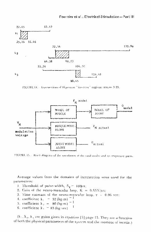
FIGURE 14

Intersections of 10 percent "iso-error " regions : test,no . 3-23.

model

FIGURE 15 . -- Block diagram of the simulation of the total model and its respective parts.

Average values from the domains of i

)r were used for theparameters:

1. Threshold of pulse-width, S 9 = I80us;2. Gain of the neuromuscular loop, K = 0 .65N/ys;3. Tirne constant of the neuro-muscular loop,

0 .06 sec;4. coefficient k, = 32 (kg-m)5. coefficient k, = 80 (kg-m)6. coefficient k 3 = 83 (kg-sec)

(k, , k 2 , k 3 are gains given in equation

1

'1 . They are a functionof both the physical parameters of the systems

the moment of inertia .

Simulation of Eh

sc lar loop using the previous values for theparameters K, and

As a close comparison between the simulatedmuscular force and the measured muscular force, Figures 16 and 17.

FIGURE 16 .-Simul

ilic elccuumechanical neuromuscular model : test no . 3-23.

Curve index x -=

put (muscular force in N) . Curve index '0) = Model Output

(muscular force in t ) . u

index Ll

Input (pulse width in /0,sec).

FIGURE 17 .-- Simulation of the electromechanical neuromuscular model : test no . 4-24.

Curve index X = Actual Output (muscular force in N) . Curve index ,(,> = Model Output

(muscular force in N) . Curve index 4.1 = Input (pulse width in 1ttsec).

DOtIOf Er

'DST NO 3-23

00101 if 10N Of

Fi,FETRD

EHANICAL PATTERN IIrr.A tnctx7tl0i. Iw.,ta

n-, 051

.4

COKE£ II) I04,sioo ionet t,

TIME IN SEC.

fl.

a a

TEST NO ‘-04

ECTRO-MECRANICAL PATTERN IR.4044t)C 1000504FE4 . NAN. 10 0 .1oR”olv 4 111ISFIIEAA FORCE 4 4 44.1

' . .

. 4A

114 40 10$E.Cc ,

TIME IN SEC.

20

Fournier et al . : Electrical Stimulation—Part 111

Figures 18 and 19 show the comparison of the output of the simulationof the complete model, simulated joint position, and the actual measuredjoint position .

amass E .

TEST NO 3-23

SIMULATION OF THE COMPLETE PATTERNSim 604.f, ,013

AMIN.

n

IN GII.ALSI

An SL C .IIWE

EAUEEN Odffl.111 11 'm.MmmN

;EbNaS:

ISM

. LIPS! ' f VIM-SE DLNA914,1 IN nlIa.C.

03

03 5

130

1 .5

2.0

FIGURE 18 . --Simulation of the complete model : test no . 3-23 . Curve index X = ActualOutput (angular displacement in degrees) . Curve index 0 = Model Output (angulardisplacement in degrees) . Curve index U = Input (pulse width inysec).

FIGURE I9 .-Simulation of the complete model : test no . 4-24 . Curve index X = ActualOutput (angular displacement in degrees) . Curve index <'), = Model Output (angular dis-placement in degrees) . Curve index F] = Input (pulse width in,Usec).

DOMDRE Em

TEST NO 4-24

SIMULATION OF THE COMPLETE PATTERNA1151 LJ,t

. nM,m‘.. 0.0E31 1m:1ml-M4 c,n,nka,ledr0 :mmELSICaNE INMEI

m PAN.FnN CJTEJT NYMJ-mM

NMInI,I;SlWI 6&J CJnC 10E2

iN,IT

EIJMNTIGNt 'N M3-6.

03

3

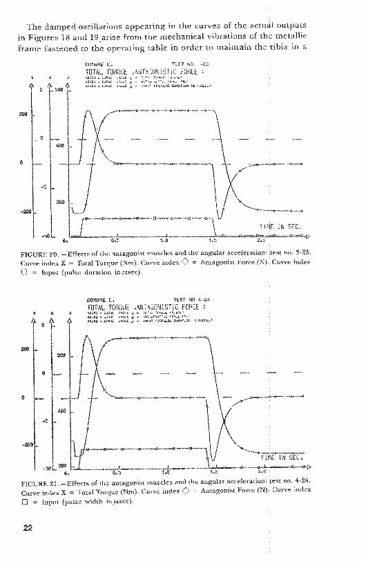
The damped oscillations appearing in the curves of the actual outputsin Figures 18 and 19 arise from the mechanical vibrations of the metallicframe fastened to the operating table in order to maintain the tibia in a

FIGURE 20 . — Effects of the antagonist muscles and the angular acceleration : test no . 3-23.

Curve index X = Total Torque (Nm) . Curve index <I) = Antagonist Force (N) . Curve index

0 = Input (pulse duration in,usec).

DOPIBFIE E .

TEST NO 4—24

TOTAL TORQUE , .ANT'AGONISTLC FORCE

. 4.4N.t 06GEt 6, 4 ,Ao rrttt,4.

ttutsa 4 40,44

4ttj 0 4

NG

ttet t

A

46143

twu 0 6 6646 t nAGAG not.4ttaN

0®

0a5

1,0

1,5

5,0

FIGURE 21 .—Effects of the antagonist muscles and the angular acceleration : test no . 4-24.

Curve index X = Total Torque (Nm) . Curve index = Antagonist Force (N) . Curve index

El = Input (pulse width in /u,sec).

DOMF01E

TEST NO .23

TOTAL TORQUE ANTACON1SfIC FORCE4115I WAG

4 %At. i'c tttt tooAAA 4 60NJ4. n 4.El 0 .

,4-40MUSS 4

itittA 0 . ;64A' lttdt t‘At GEA?W% 455 4,AG.,

22

Fournier et ales Electrical Stimulation-Part 111

fixed horizontal position . They do not appear in the simulated model . Thesteady states, during stimulation and when it is over, are identical in boththe actual and simulated outputs.

Figures 20 and 21 show the simulated effects of the antagonist musclesand the angular acceleration.

CONCLUSION

The control law of a physical system must define a realistic mathemati-cal model of the process and also provide a model simple enough to beuseful . The proposed model satisfies these two criteria . The results of thesimulation show that, with a single stimulation signal, the actual and thesimulated outputs behave in an identical manner . Hence, theidentification procedure has provided a sufficient estimation of theparameters of the system, thus obviating the necessity of determiningbiomechanical constants by complex and inaccurate measurements.Although progress yet remains to be made in the surgical area (e .g., inimplantation of electrodes and achieving tolerance by the human body)we have defined the steps for the position control of an articulatedsystem.

From the proposed model, it becomes possible to design an analogfeedback control loop for a position servo-system and to stabilize the jointposition when the external load is opposed to the agonist muscle's force.If the external load is variable, agonist and antagonist muscle groups ofthe joint have to be simultaneously involved . The previous identificationprocedure is still valid for each muscle group but problems of synergy ofseveral muscular contraction effects arise . When the control of severalcoupled joints is considered, as in legged-locomotion problems, thelogical level of synergy becomes more complex . A theoretical approach tothese problems is being studied in our laboratory.

ACKNOWLEDGMENTS

The authors wish to express their gratitude to Professor P . Rabischongand E. Peruchon for useful discussions during this work . Also, they thankF. Bonnet for surgical assistance.

REFERENCES

L Marx, C . : Le Neurone, Physiologie : Systeme Nerveux, Muscle . Charles Kayser, Tome2, Chap . 1, p 7.

2 . Lievremont, M . : Contribution a 1'Etude de la Jonction Neuromusculaire . These d'Etat,Universite de Paris, June 1972.

3a . Aubert, X . : Le muscle strie, Physiologic : Systeme Nerveux, Muscle . Charles Kayser,Tome 2, Chap . 19, p 1261.

b . Scherrer, J . : Physiologic de la Musculature Striee Squelettique chez l ' Homme,Physiologic : Systeme Nerveux, Muscle . Charles Kayser, Tome 2, Chao . 20 . D 1325 .

4. Rabischong, P . et al . : Basic Studies in Electrical Stimulation of Limbs—Part1 .—Method and Approach . Bull . Prosthetics Res ., 10-22, Fall 1974.

5. Rabischong, P . et al . : Basic Studies in Electrical Stimulation of Limbs—Part 2 .—OpenLoop Control of Muscular Contraction . Bull . Prosthetics Res ., 10-22 Fall 1974.

6. Pertuzon, E . : La Contraction Musculaire dans le Mouvement Volontaire Maximal.These d'Etat, Universite des Sciences et Techniques de Lille, June 1972.

7. Dombre, E . : Commande en Position d'un Levier Squelettique par Stimulation Ner-veuse . These de 3e cycle, Montpellier, Mar . 1975.

8. Drillis, R ., R . Contini, M . Bluestein : Body Segment Parameters . Artificial Limbs,8(1) :44-66, Spring 1969.

9. De Larminat, P . : Sur l'Identification par filtrage non lineaire, These d'Etat,Universitede Nantes, May 1971.

10. Nahi, N .E . : Estimation Theory and Applications . John Wiley and Sons, New York1969.

11. Richalet, J ., A . Rault, and R . Pouliquen : Identification des Processus par la Methodedu MOdele . Gordon and Breach, 1971.

12. Graupe, D . : Indentification of Systems . Van Nostrand Reinhold Co ., New York 1972.13. Bellman, R .E . and S .E . Dreyfus : Applied Dynamic Programming . Princeton Universi-

ty Press, Princeton, N .J . 1962.14. Gugie., P ., A . Trnkoczy, and U . Stanie : Hybrid Control of the Ankle Joint . Proceedings

of the Fourth International Symposium on External Control of Human Extremities,Dubrovnik, pp . 617-631, Aug. 1972.

15. Liegeois, A . and A . Fournier : Modelisation et Commandabilite de la LocomotionArtificielle . Symposium sur l'Identification des Systemes Dynamiques Humains dansles Processus Homme-Machine, Lille, May 12-15, 1975.

24