Fourier Kernel Learning

Eduard Gabriel Bazavan1, Fuxin Li2, and Cristian Sminchisescu3,1

1 Institute of Mathematics of the Romanian Academy2 College of Computing, Georgia Institute of Technology

3 Faculty of Mathematics and Natural Science, University of Bonneduard.bazavan@imar.ro, fli@cc.gatech.edu,cristian.sminchisescu@ins.uni-bonn.de

Abstract. Approximations based on random Fourier embeddings haverecently emerged as an efficient and formally consistent methodology todesign large-scale kernel machines [23]. By expressing the kernel as aFourier expansion, features are generated based on a finite set of ran-dom basis projections, sampled from the Fourier transform of the kernel,with inner products that are Monte Carlo approximations of the originalnon-linear model. Based on the observation that different kernel-inducedFourier sampling distributions correspond to different kernel parameters,we show that a scalable optimization process in the Fourier domain canbe used to identify the different frequency bands that are useful for pre-diction on training data. This approach allows us to design a family oflinear prediction models where we can learn the hyper-parameters of thekernel together with the weights of the feature vectors jointly. Underthis methodology, we recover efficient and scalable linear reformulationsfor both single and multiple kernel learning. Experiments show that ourlinear models produce fast and accurate predictors for complex datasetssuch as the Visual Object Challenge 2011 and ImageNet ILSVRC 2011.

1 Introduction

The proper choice of kernel function and its hyper-parameters are crucial tothe success of kernel methods in practical applications. These selections span anumber of different problems, from choosing a single width parameter in radialbasis kernels, scaling feature dimensions with different weights [6], to learninga linear or a non-linear combination of multiple kernels (MKL) [17]. In compli-cated practical problems such as computer vision, sometimes the need of multiplekernels arises naturally [32]. Images can be represented using descriptors basedon shape, color and texture, and these descriptors have different roles in clas-sifying different visual categories. In such situations it is, in principle, easy todesign a classifier where each kernel operates on one of the descriptors or featurechannels and the classifier is obtained as a combination of kernels with categorydependent learnt weights.

A natural difficulty in kernel learning is scalability. Kernel methods scale withan already mediocre time complexity of at least O(N2.3) with respect to the size

2 Eduard Gabriel Bazavan, Fuxin Li, and Cristian Sminchisescu

N of the training set, but combining multiple kernels or learning the hyper-parameters of a single kernel significantly slows down training. Some speed-upsapply to specific kernels, but only in limited scenarios [22]. As a consequence,some of the standard kernel learning approaches can only handle a few thousandtraining examples at most. This is insufficient for the current age of massivedatasets, such as the 11 million images ImageNet, or the 19 million articleswithin Wikipedia.

An emerging technique that can in principle speed up the costly kernelmethod while at the same time preserving its non-linear predictive power isthe random Fourier feature methodology (RFF) [23, 33, 19]. By sampling com-ponents from the frequency space of the kernel using Monte Carlo methods, RFFobtains a bounded, approximate representation of a kernel embedding, even fornon-linear models that may span an infinite-dimensional space. Many operationsare simplified once such a representation is available, the most notable being thatany kernel learning algorithm would now scale as O(N), where N is the num-ber of examples. This opens path for applying kernel methods to the realm ofmassive datasets.

In the seminal work on random Fourier approximations [23], the method-ology was developed primarily for radial basis kernels. Recent work [33, 19, 25]focused on extending this technique to other useful kernels defined on histogramfeatures (empirical estimates of multinomial distributions), such as the χ2 andthe histogram intersection measures. However, the potential of the linear Fouriermethodology for kernel learning remains largely unexplored. In this paper wedevelop the methodology for learning both single kernel and for multiple ker-nel combinations in the Fourier domain and show that these models produceaccurate and efficient predictors. We conduct experiments in the visual objectrecognition domain, using both the PASCAL Visual Object Challenges 2011 andthe ImageNet ILSVRC 2011 datasets, to illustrate the performance of the pro-posed Fourier kernel learning methodology. We also compare against non-linearlearning algorithms, designed to operate in the original kernel space and showsignificant speedups at comparable accuracy.

2 Related work

Approaches to kernel learning can be broadly classified into methods that es-timate the hyper-parameters of a single kernel[6, 15] and methods that esti-mate the weights of a linear combination of kernels and possibly their hyper-parameters – the multiple kernel learning framework, MKL[2, 16, 34].

A popular approach for single kernel learning is the gradient-based methodpursued by Chapelle et al. [6, 15]. Keerthi et al. [15] give an efficient algorithmthat alternates between learning an SVM and optimizing the feature weights.Cortes et al. [8] propose a two-stage method based on the modification of akernel alignment [9] metric and prove a number of learning bounds. Approachesto single kernel learning under a kernel prior have been pursued both as semi-definite programs[17] and within unconstrained optimization formulations[12],

Fourier Kernel Learning 3

although in both cases the optimization is fairly involved and the complexityremains an issue. More recent methods attempt to track the entire regularizationpath in the non-linear case [20].

Multiple kernel learning provides a powerful conceptual framework for bothmodel combination and model selection and has attracted significant researchrecently. Initial approaches, originating with work by Lanckriet et al. [17] es-timated a linear combination of kernels using semi-definite programming. Thiswas reformulated by Bachet al. [3] as block-norm regularization, reducing the op-timization problem to a second order cone program applicable to medium scaleproblems. More recent methods [7] learn a polynomial combination of kernels.A number of approaches have pursued different lp-norms for kernel selection [16,34]. Hierarchical kernel learning approaches like (HKL) [2] perform feature selec-tion combinatorially, by choosing kernel combinations obtained by mapping to adirected acyclic graph. The search for such combinations can then be performedin polynomial time.

A difficulty with many single or multiple kernel learning formulations is theirrelatively unfavorable scaling properties. When kernels are used, such methodsusually scale at least quadratically in the number of examples. Sometimes scalingin the combined number of kernel parameters and number of kernel models canalso become an issue. A formulation of kernel learning within a linear Fourierframework, as pursued in this paper, carries the promise of better scalabilityand wider applicability to large datasets, while at the same time preserving thenon-linear predictive power that makes kernel methods attractive.

3 Learning Kernels in the Random Fourier Domain

3.1 Random Fourier Approximations

Kernels offer substantial power and flexibility to predictive models. Central totheir use is the ‘kernel trick’ which allows the design of algorithms that dependonly on the inner product of their arguments. This is based on the propertyof positive definite kernels k(·, ·) to define a lifting φ so that the inner productbetween lifted data points can be efficiently computed as φ(x)>φ(y) = k(x,y),without having to explicitly construct φ(x). Algorithms become linear in a com-plex feature space induced by φ, but access the data only through evaluationsof the kernel k in input space. This makes possible to handle complex or infinitedimensional feature space mappings φ, and indeed these usually give the bestresults in visual recognition datasets [14, 18]. However the very advantage thatmake kernel methods popular – the kernel trick, requires the manipulation ofmatrices of pairwise examples. For large datasets, the scaling of kernel methodsis at least quadratic in the number of examples. This makes their direct usageimpractical beyond datasets of 104 elements. The methodology we pursue is toapproximate the kernel function linearly using random feature maps.

Key to the random Fourier methodology is Bochner’s theorem, that connectspositive definite kernels and their Fourier transforms [26, 23, 19]. For positive def-inite translation-invariant kernels k(x,y) = k(x−y) on Rm, Bochner’s theorem

4 Eduard Gabriel Bazavan, Fuxin Li, and Cristian Sminchisescu

kernel parametric probability quantile σh(ω)form (kσ) distribution µk(γ)

Gaussian 1

σ√2πe− ‖x−y‖

2

2σ2σ√2πe−

σ2γ2 σ

√2erf−1(2ω − 1)

Skewed− χ22(x+c)σ(y+c)σ

(x+c)2σ+(y+c)2σ12σ

sech(πγ2σ

)σ 2π

log(tan

(π2ω))

Skewed Intersection min{

(x+c)σ

(y+c)σ, (y+c)σ

(x+c)σ

}1π

σσ2+γ2

σ tan(π(ω − 1

2))

Table 1. Examples of kernels that can be efficiently optimized within our framework,given for the unidimensional case. In the multidimensional case, the Fourier methodol-ogy decomposes, hence it requires a simple multiplication of parameters correspondingto each dimension. Above, the random variable ω is drawn from the uniform distribu-tion.

guarantees that every kernel is the inverse Fourier transform of a proper prob-

ability distribution µk. Defining ζ(x) = ejγ>x (with j the imaginary unit), the

following equality holds:

kσ(x,y) =

∫Rm

ejγ>(x−y)µk(γ)dγ = Eµk [ζγ(x)ζγ(y)∗] ≈ ψΓ (x)>ψΓ (y) (1)

where ∗ is the (complex) conjugate, and

ψΓ (x) =

√2

d

[cos(γ>i x + 2πbi

)]i=1,d

∈ Rd×1 (2)

is the random feature map at samples Γ = {γ1, . . . ,γd} drawn from µk andb ∼ U[0, 1], the uniform distribution in the interval [0, 1]. We approximate theexpectation Eµk [ζγ(x)ζγ(y)∗] by means of a Monte-Carlo sample drawn from thedistribution µk. This is an operation on linear functions with explicit features.The algorithm for the change of representation has two steps: i) Generate drandom samples Γ from the distribution µk; ii) Compute the random projectionψΓ using (2), for all training examples. The approximation has the convergencerate of Monte Carlo methods, O(d−1/2), dependent on the random sample size,but independent of the input dimension. One usually needs up to a few thousanddimensions to approximate the original kernel accurately.

Our kernel learning approach is based on the observation that manipulatingthe sampling distribution µk in an optimization process identifies the differentfrequency bands that are useful for prediction on training data. This effectivelyleads to a posterior frequency distribution, given µk as a prior. Generating sam-ples from this posterior and optimizing with respect to their expectation on thetraining set gives a direct way of learning the parameters of the kernel in theFourier domain. However, as the kernel hyper-parameters σ change, Γ (the dis-tribution induced by the kernel) changes and needs to be re-sampled. Althoughthis is feasible, changing the sampling distribution introduces conceptual dif-ficulties during optimization as sampling introduces noise, high-variance andnon-smoothness in the optimization cost. Importance sampling can be used toavoid resampling at each step, but if the parameterized frequency distribution

Fourier Kernel Learning 5

µk drifts far away from the initial kernel-induced distribution, the original sam-ples will have little importance weights, and resampling would potentially benecessary for convergence. Such difficulties can be overcome for several interest-ing kernels that belong to a class of functions where µk has an explicit quantilewhich is linear in the kernel parameters. Assuming the quantile of µk has theform γ = σ � h(ω) where h is a nonlinear function, and � is the Hadamardproduct of two vectors then we can draw the required samples Γ from µk usingthe following procedure: (i) draw d vectors ωi of the same dimensionality asthe input vectors x from the uniform distribution; (ii) pass each ωi through thenonlinearity h, and (iii) multiply each dimension of the resulting h(ωi) with thecorresponding σi. The desired samples are obtained as

γi = σ � h(ωi) (3)

Notice that when changing the kernel parameters σ we no longer have to re-sample ωi. Throughout the entire optimization process, sampling needs to bedone only once from the uniform distribution for each ωi. When σ is changed,samples from the new distribution are generated automatically from the storedvalues of h(ωi). In the sequel, we consider the case of anisotropic input scaling.In this case we have γi = [σ1h(ωi,1), . . . , σrh(ωi,r)], and the Fourier embeddingcan be written as

ψσ(x) =

√2

d

cos

r∑j=1

σjh(ωi,j)>xj + 2πbi

i=1,d

∈ Rd×1 (4)

where xj is the block from the input data x that corresponds to σi, and r is thenumber of blocks x is split into. Examples of kernels that can be learned usingthis procedure are the Gaussian, the generalized Skewed-χ2 and the generalizedSkewed Intersection[19] (see Table 1).

3.2 General Learning Model

We express our kernel learning model as a general cost optimization problemwhere we jointly learn the kernel parameters σ and the weights w of a linearpredictor operating on the new Fourier representation. In the sequel we denote Xand y the matrix of inputs or covariates x (column-wise organized) and y the vec-tor of targets on the training set, respectively. We define ψσ(X) ∈ Rd×n, where nis the number of inputs, to be the feature map applied to all inputs(columns) ofmatrix X ∈ Rm×n. The general form of the error function we wish to minimizecan be written as

f (σ,w) = l(ψσ(X)>w,y) + ν(w) + η(σ) (5)

where ψσ(x) is the Fourier embedding of an input data x, l(y,y) is the lossfunction which measures how close the predicted labels y = ψσ(X)>w are tothe ground truth y, ν(w) is a regularizer on the linear parameters w and η(σ)is a regularizer on the kernel hyper-parameters σ.

6 Eduard Gabriel Bazavan, Fuxin Li, and Cristian Sminchisescu

Optimizing the parameters in equation (5) depends on the different designdecisions made for the model. In Table 2 we show different choices of loss func-tions and regularization terms. If f is smooth in both σ and w and we choose tojointly optimize all parameters, we will need to compute the gradient of f withrespect to these parameters. The following derivatives are completely general,based on the model (5)

∂f (σ,w)

∂σ=

(∂l(ψσ(X)>w,y

)∂ψσ(X)>w

)>∂ψσ(X)>

∂σw +

∂η(σ)

∂σ(6)

∂f (σ,w)

∂w=

(∂l(ψσ(X)>w,y

)∂ψσ(X)>w

)>ψσ(X) +

∂ν(w)

∂w(7)

In the above equations, the derivative of the loss with respect to the linearpredictor ψσ(X)>w, as well as the derivatives of the regularizers are usuallyeasy to compute. A key quantity is the derivative of the random Fourier map

with respect to the parameters ∂ψσ(X)>

∂σ , e.g. (11).The number of parameters for the joint optimization can be large (up to

thousands) which indicates that a limited memory quasi Newton algorithm, suchas l-bfgs is appropriate. When f is not smooth because of specific choices ofregularization, e.g. l1 norms, it is possible to use methods based on projectiononto the constraint set instead [21]. In such cases, we only need to provide thederivative of l with respect to σ and w.

There are situations when, given σ, there is a closed form solution for w.Then we can follow an optimization scheme for σ, and at each gradient stepprovide the solution for w. In such sitations, we might also have to provide aderivative of w with respect to σ. Denote by wσ the w that minimizes f givena fixed σ. Then we have to provide the following gradient

∂f (σ)

∂σ=

(∂l(ψσ(X)>wσ,y

)∂ψσ(X)>wσ

)>(∂ψσ(X)>

∂σwσ + ψσ(X)>

∂wσ

∂σ

)+

(∂ν(wσ)

∂wσ

)>∂wσ

∂σ+∂η(σ)

∂σ(8)

Such methods are applicable not only for random Fourier feature maps, butfor any other embeddings where it is easy to compute the gradient of the map∂ψσ(X)∂σ with respect to the parameters.In the next sections we present two models that we find particularly effective

for visual applications. Each one has an equivalent non-approximated counter-part which scales quadratically in the number of training samples, whereas ourFourier reformulations have linear complexity.

3.3 Single Kernel Learning

First we consider the case of single kernel learning. We use the Fourier embeddingψσ, introduced earlier (4) as our approximation of the kernel lifting. This model

Fourier Kernel Learning 7

l(y,y) ν(w) η(σ)

square loss: ‖y − y‖22 l2: λ‖w‖22 l2: ν‖σ‖22hinge loss:

∑i max(yi − yi, 0) l1: λ‖w‖1 l1: ν‖σ‖1

logistic loss:∑i log(1 + exp(−yiyi)) l2,1: λ

∑j ‖wj‖2

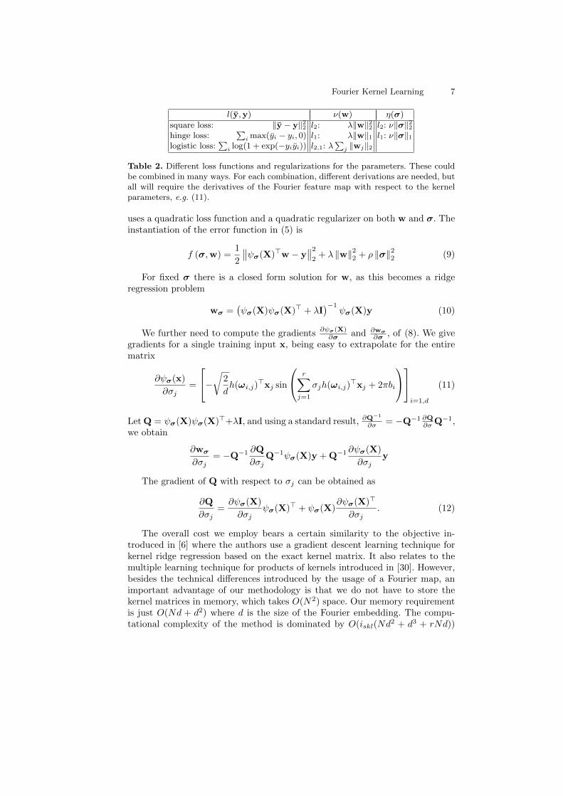
Table 2. Different loss functions and regularizations for the parameters. These couldbe combined in many ways. For each combination, different derivations are needed, butall will require the derivatives of the Fourier feature map with respect to the kernelparameters, e.g. (11).

uses a quadratic loss function and a quadratic regularizer on both w and σ. Theinstantiation of the error function in (5) is

f (σ,w) =1

2

∥∥ψσ(X)>w − y∥∥2

2+ λ ‖w‖22 + ρ ‖σ‖22 (9)

For fixed σ there is a closed form solution for w, as this becomes a ridgeregression problem

wσ =(ψσ(X)ψσ(X)> + λI

)−1ψσ(X)y (10)

We further need to compute the gradients ∂ψσ(X)∂σ and ∂wσ

∂σ , of (8). We givegradients for a single training input x, being easy to extrapolate for the entirematrix

∂ψσ(x)

∂σj=

−√2

dh(ωi,j)

>xj sin

r∑j=1

σjh(ωi,j)>xj + 2πbi

i=1,d

(11)

Let Q = ψσ(X)ψσ(X)>+λI, and using a standard result, ∂Q−1

∂σ = −Q−1 ∂Q∂σ Q−1,

we obtain

∂wσ

∂σj= −Q−1 ∂Q

∂σjQ−1ψσ(X)y + Q−1 ∂ψσ(X)

∂σjy

The gradient of Q with respect to σj can be obtained as

∂Q

∂σj=∂ψσ(X)

∂σjψσ(X)> + ψσ(X)

∂ψσ(X)>

∂σj. (12)

The overall cost we employ bears a certain similarity to the objective in-troduced in [6] where the authors use a gradient descent learning technique forkernel ridge regression based on the exact kernel matrix. It also relates to themultiple learning technique for products of kernels introduced in [30]. However,besides the technical differences introduced by the usage of a Fourier map, animportant advantage of our methodology is that we do not have to store thekernel matrices in memory, which takes O(N2) space. Our memory requirementis just O(Nd + d2) where d is the size of the Fourier embedding. The compu-tational complexity of the method is dominated by O(iskl(Nd

2 + d3 + rNd))

8 Eduard Gabriel Bazavan, Fuxin Li, and Cristian Sminchisescu

where d is the size of the random Fourier features, N is the number of trainingsamples, r is the number of kernel hyper-parameters and iskl is the number ofiterations to convergence. O(Nd2 + d3) is the cost of computing the matrix Qand inverting it.

3.4 Multiple Kernel Learning

We propose a multiple kernel learning formulation where the feature channels areinitially transformed using random Fourier embeddings and concatenated withinan optimization framework based on block l1 norm regularizer (RFF-MKL).We prove that this new formulation is equivalent to an l1 regularized multiplekernel learning formulation introduced in [30] (GMKL) and then compare thetwo methodologies. Experiments show that both approaches have similar per-formance. In contrast, the block l1 regularized MKL method based on randomFourier maps runs faster and scales better since we do not need to compute orstore the Gram matrices associated with the input features.

In this case, the Fourier embedding has the following concatenated form

ψσ(X) =[ψσ1(X1)>, . . . , ψσr (Xr)

>]> where we have split row-wise the inputmatrix X into r different input matrices {X1, . . . ,Xr}, one corresponding toeach feature channel. We have a different embedding for each descriptor

ψσj (Xj) =

[√2

dcos(σjh(ωi,j)

>Xj + 2πbi)]i=1,d

∈ Rd×n (13)

and for different input samples u and v on which the same anisotropic scalingis applied we have ψσ(u)>ψσ(v) =

∑ri=1 ψσi(ui)

>ψσi(vi) ≈∑ri=1 kσi(ui,vi).

This corresponds to the sum of kernels for the different feature channels.We now show that the l1 regularized GMKL is equivalent, as an optimiza-

tion procedure, with RFF-MKL. For GMKL, we have the following primal prob-lem[30]

minw,d

1

2w>w + Cl(φ(X)>w,y) +

r∑j=1

dj , subject to d ≥ 0 (14)

where l is the ε-insensitive hinge loss used for svm regression and

φ(X) = [√d1φ1(X1)>, . . . ,

√drφr(Xr)

>]>, (15)

with φj(Xj) the lifting associated to kernel kj , which is applied on the featurechannel Xj . From the Representer Theorem [27] we know that the solution forw will be a linear combination of basis functions

w =∑

αxφ(x) =[√

d1w>1 , . . . ,

√drw

>r

]>(16)

where we have summed over all input data x and dropped the bias term forsimplicity. We can then rewrite the above equation (14) as

minw,d

r∑j=1

dj2‖wj‖22 + Cl(

r∑j=1

djφj(Xj)>wj ,y) +

r∑j=1

dj , subject to d ≥ 0 (17)

Fourier Kernel Learning 9

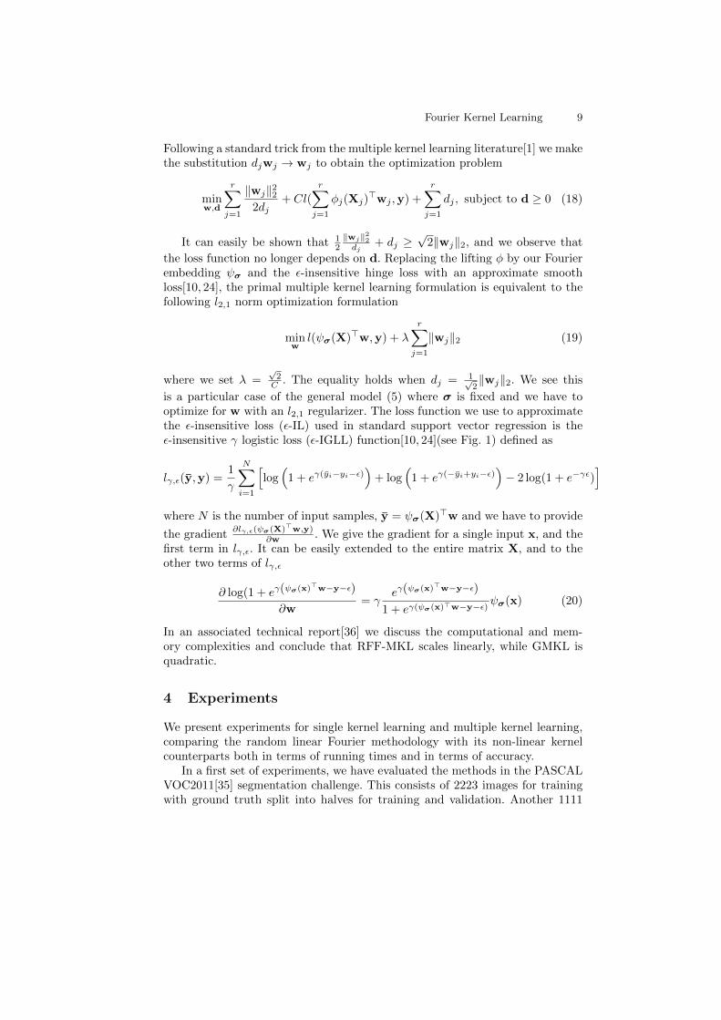
Following a standard trick from the multiple kernel learning literature[1] we makethe substitution djwj → wj to obtain the optimization problem

minw,d

r∑j=1

‖wj‖222dj

+ Cl(

r∑j=1

φj(Xj)>wj ,y) +

r∑j=1

dj , subject to d ≥ 0 (18)

It can easily be shown that 12‖wj‖22dj

+ dj ≥√

2‖wj‖2, and we observe that

the loss function no longer depends on d. Replacing the lifting φ by our Fourierembedding ψσ and the ε-insensitive hinge loss with an approximate smoothloss[10, 24], the primal multiple kernel learning formulation is equivalent to thefollowing l2,1 norm optimization formulation

minw

l(ψσ(X)>w,y) + λ

r∑j=1

‖wj‖2 (19)

where we set λ =√

2C . The equality holds when dj = 1√

2‖wj‖2. We see this

is a particular case of the general model (5) where σ is fixed and we have tooptimize for w with an l2,1 regularizer. The loss function we use to approximatethe ε-insensitive loss (ε-IL) used in standard support vector regression is theε-insensitive γ logistic loss (ε-IGLL) function[10, 24](see Fig. 1) defined as

lγ,ε(y,y) =1

γ

N∑i=1

[log(

1 + eγ(yi−yi−ε))

+ log(

1 + eγ(−yi+yi−ε))− 2 log(1 + e−γε)

]where N is the number of input samples, y = ψσ(X)>w and we have to provide

the gradient∂lγ,ε(ψσ(X)>w,y)

∂w . We give the gradient for a single input x, and thefirst term in lγ,ε. It can be easily extended to the entire matrix X, and to theother two terms of lγ,ε

∂ log(1 + eγ(ψσ(x)>w−y−ε)

∂w= γ

eγ(ψσ(x)>w−y−ε)

1 + eγ(ψσ(x)>w−y−ε)ψσ(x) (20)

In an associated technical report[36] we discuss the computational and mem-ory complexities and conclude that RFF-MKL scales linearly, while GMKL isquadratic.

4 Experiments

We present experiments for single kernel learning and multiple kernel learning,comparing the random linear Fourier methodology with its non-linear kernelcounterparts both in terms of running times and in terms of accuracy.

In a first set of experiments, we have evaluated the methods in the PASCALVOC2011[35] segmentation challenge. This consists of 2223 images for trainingwith ground truth split into halves for training and validation. Another 1111

10 Eduard Gabriel Bazavan, Fuxin Li, and Cristian Sminchisescu

images are given for testing without ground truth. Following the standard pro-cedure we have trained the methods on the training set (further split, internallyinto training and validation for kernel hyper-parameter learning) and tested onthe PASCAL VOC2011 validation set. We have used the methodology presentedin Li et al. [18] and relied on the publicly available CPMC segmentation algo-rithm from Carreira and Sminchisescu [4] to filter the initial pool of segmentsto around 100 segments per image. For each of these segments we extracted 7types of features among which two bag of visual words for color SIFT [29] andtwo dense gray scale SIFT descriptors, one on each segment and one on thebackground of each segment and three types of phog descriptors, two on the Pbedges given by [13] computed at different scales, one on the contour and one onthe foreground. The third phog descriptor does not use Pb. Because the numberof segments (around 105) was still too large for any kernel support vector basedalgorithm to cope with, we have chosen up to 104 segments for each class. Thesegments were chosen based on their individual scores and we balanced the ex-amples to have a fair split between positives and negatives. More detail on howthe scores are defined and computed can be found in [18].

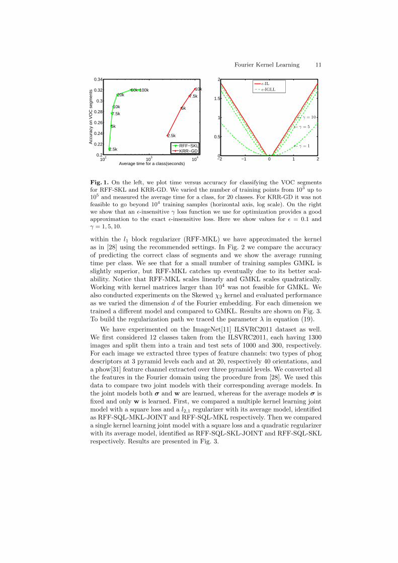
Single Kernel Learning. We run a set of experiments for our single kernellearning technique based on random Fourier features (RFF-SKL) and comparein terms of accuracy with the single kernel learning technique introduced byChapelle et al. [6] (KRR-GD). We want to predict the class for more than 105

segments. We expect RFF-SKL to give comparable results in terms of accuracyto KRR-GD. Results are shown in Table 3. We vary the size of the trainingset from 103 to 105 and measure both the running times of RFF-SKL and theaccuracy. In Fig. 1 we show how the accuracy depends on the size of the trainingdata and the average time required for RFF-SKL and KRR-GD to run on oneclass. We observe that RFF-SKL running time scales linearly in the number ofexamples. The number of random Fourier samples we have chosen was d = 3000.This is consistent with our computational complexity discussed in Section 3.3.We are able to tune the hyper-parameters of a Fourier model trained with morethan 105 samples, each with 3000 attributes in less than 15 minutes.

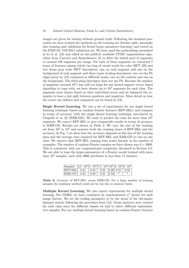
Samples 2.5 · 103 5 · 103 7.5 · 104 104 2 · 104 6 · 104

RFF-SKL 0.21 0.25 0.28 0.29 0.31 0.32

KRR-GD 0.24 0.29 0.31 0.32 * *

Table 3. Accuracy of RFF-SKL versus KRR-GD. For a large number of trainingsamples the nonlinear method could not be run due to memory limits.

Multiple Kernel Learning. We also report experiments for multiple kernellearning. For GMKL we have evaluated an exponentiated χ2 kernel for eachimage feature. We set the scaling parameter to be the mean of the chi-squaredistance matrix following the procedure from [14]. Gram matrices were createdfor each class since for different classes we had to select different representa-tive samples. For our multiple kernel learning based on random Fourier features

Fourier Kernel Learning 11

102

103

104

0.2

0.22

0.24

0.26

0.28

0.3

0.32

0.34

2.5k

5k

7.5k

10k

20k60k 100k

2.5k

5k

7.5k

10k

Average time for a class(seconds)

Acc

urac

y on

VO

C s

egm

ents

RFF−SKLKRR−GD

−2 −1 0 1 20

0.5

1

1.5

2

← γ = 1

← γ = 5

← γ = 10

ε-IL

ε-IGLL

Fig. 1. On the left, we plot time versus accuracy for classifying the VOC segmentsfor RFF-SKL and KRR-GD. We varied the number of training points from 103 up to105 and measured the average time for a class, for 20 classes. For KRR-GD it was notfeasible to go beyond 104 training samples (horizontal axis, log scale). On the rightwe show that an ε-insensitive γ loss function we use for optimization provides a goodapproximation to the exact ε-insensitive loss. Here we show values for ε = 0.1 andγ = 1, 5, 10.

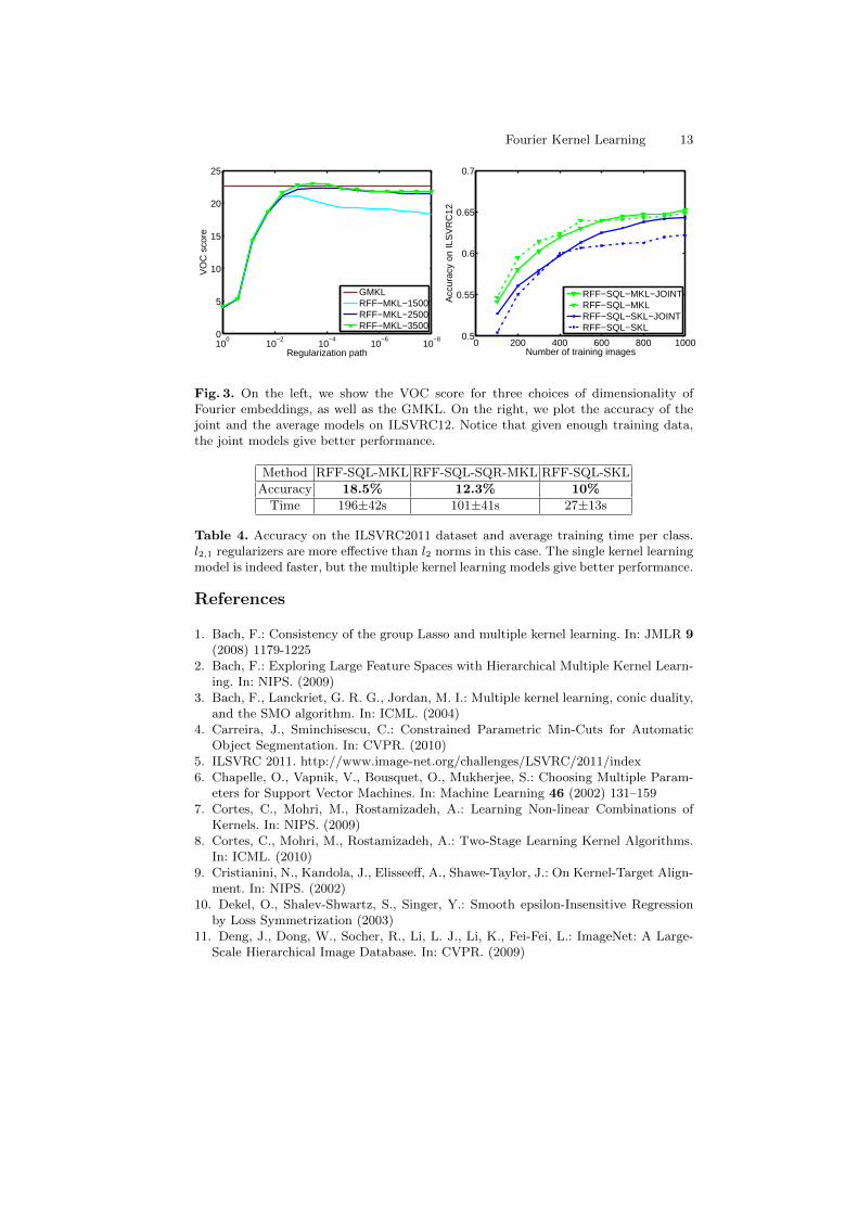
within the l1 block regularizer (RFF-MKL) we have approximated the kernelas in [28] using the recommended settings. In Fig. 2 we compare the accuracyof predicting the correct class of segments and we show the average runningtime per class. We see that for a small number of training samples GMKL isslightly superior, but RFF-MKL catches up eventually due to its better scal-ability. Notice that RFF-MKL scales linearly and GMKL scales quadratically.Working with kernel matrices larger than 104 was not feasible for GMKL. Wealso conducted experiments on the Skewed χ2 kernel and evaluated performanceas we varied the dimension d of the Fourier embedding. For each dimension wetrained a different model and compared to GMKL. Results are shown on Fig. 3.To build the regularization path we traced the parameter λ in equation (19).

We have experimented on the ImageNet[11] ILSVRC2011 dataset as well.We first considered 12 classes taken from the ILSVRC2011, each having 1300images and split them into a train and test sets of 1000 and 300, respectively.For each image we extracted three types of feature channels: two types of phogdescriptors at 3 pyramid levels each and at 20, respectively 40 orientations, anda phow[31] feature channel extracted over three pyramid levels. We converted allthe features in the Fourier domain using the procedure from [28]. We used thisdata to compare two joint models with their corresponding average models. Inthe joint models both σ and w are learned, whereas for the average models σ isfixed and only w is learned. First, we compared a multiple kernel learning jointmodel with a square loss and a l2,1 regularizer with its average model, identifiedas RFF-SQL-MKL-JOINT and RFF-SQL-MKL respectively. Then we compareda single kernel learning joint model with a square loss and a quadratic regularizerwith its average model, identified as RFF-SQL-SKL-JOINT and RFF-SQL-SKLrespectively. Results are presented in Fig. 3.

12 Eduard Gabriel Bazavan, Fuxin Li, and Cristian Sminchisescu

103

104

105

0.25

0.3

0.35

Number of training samples

Acc

urac

y on

VO

C s

egm

ents

RFF−MKLGMKL

0 1 2 3 4 5 6

x 104

0

500

1000

1500

2000

2500

3000

3500

4000

Number of training samples

Tot

al r

unni

ng ti

me

per

clas

s

RFF−MKLGMKL

Fig. 2. On the left, we show the accuracy for classifying the VOC segments for RFF-MKL and GMKL, as a function of the number of training examples. RFF-MKL scalessignificantly better than GMKL. On the right, we show running times expressed inseconds for RFF-MKL and GMKL. Notice that RFF-MKL scales linearly whereasGMKL scales quadratically. Error-bars are obtained by averaging over the number ofclasses (20 in this case).

We then extracted the same feature channels for all the 1000 classes of theILSVRC2011 dataset. We trained in the Fourier domain RFF-SQL-MKL, RFF-SQL-SKL and a third multiple kernel learning model with l2 loss and l2 regu-larizer, identified as RFF-SQL-SQR-MKL, on the entire dataset. We tested onthe 50,000 images validation set, since the ground truth for the test set is notpublicly available. Results are shown in Table 4. We observe that our resultsmatch the accuracy levels reported for Imagenet baselines [5]. While better fea-tures and kernels can certainly improve performance, we appreciate that fast,yet generic approximate non-linear learning methods like the ones we propose,have potential for such large datasets.

5 Conclusions

The Fourier methodology provides a powerful and formally consistent class oflinear approximations for non-linear kernel machines, carrying the promise ofboth good model scalability and non-linear prediction power. This has motivatedresearch in extending the class of useful kernels that can be approximated, e.g.χ2 [33, 19, 25], but leaves ample space for reformulating standard problems likesingle or multiple kernel learning in the linear Fourier domain. In this paper, wehave developed gradient-based methods for single and multiple-kernel learningin the Fourier domain and showed that these are efficient and produce accurateresults on complex computer vision datasets like VOC2011 and ILSVRC2011. Infuture work we plan to explore alternative kernel map approximations, featureselection and non-convex optimization techniques for learning.Acknowledgements: This work was supported by CNCS-UEFICSDI, underPNII RU-RC-2/2009, PCE-2011-3-0438, and CT-ERC-2012-1.

Fourier Kernel Learning 13

10−8

10−6

10−4

10−2

100

0

5

10

15

20

25

Regularization path

VO

C s

core

GMKLRFF−MKL−1500RFF−MKL−2500RFF−MKL−3500

0 200 400 600 800 10000.5

0.55

0.6

0.65

0.7

Number of training images

Acc

urac

y on

ILS

VR

C12

RFF−SQL−MKL−JOINTRFF−SQL−MKLRFF−SQL−SKL−JOINTRFF−SQL−SKL

Fig. 3. On the left, we show the VOC score for three choices of dimensionality ofFourier embeddings, as well as the GMKL. On the right, we plot the accuracy of thejoint and the average models on ILSVRC12. Notice that given enough training data,the joint models give better performance.

Method RFF-SQL-MKL RFF-SQL-SQR-MKL RFF-SQL-SKL

Accuracy 18.5% 12.3% 10%

Time 196±42s 101±41s 27±13s

Table 4. Accuracy on the ILSVRC2011 dataset and average training time per class.l2,1 regularizers are more effective than l2 norms in this case. The single kernel learningmodel is indeed faster, but the multiple kernel learning models give better performance.

References

1. Bach, F.: Consistency of the group Lasso and multiple kernel learning. In: JMLR 9(2008) 1179-1225

2. Bach, F.: Exploring Large Feature Spaces with Hierarchical Multiple Kernel Learn-ing. In: NIPS. (2009)

3. Bach, F., Lanckriet, G. R. G., Jordan, M. I.: Multiple kernel learning, conic duality,and the SMO algorithm. In: ICML. (2004)

4. Carreira, J., Sminchisescu, C.: Constrained Parametric Min-Cuts for AutomaticObject Segmentation. In: CVPR. (2010)

5. ILSVRC 2011. http://www.image-net.org/challenges/LSVRC/2011/index6. Chapelle, O., Vapnik, V., Bousquet, O., Mukherjee, S.: Choosing Multiple Param-

eters for Support Vector Machines. In: Machine Learning 46 (2002) 131–1597. Cortes, C., Mohri, M., Rostamizadeh, A.: Learning Non-linear Combinations of

Kernels. In: NIPS. (2009)8. Cortes, C., Mohri, M., Rostamizadeh, A.: Two-Stage Learning Kernel Algorithms.

In: ICML. (2010)9. Cristianini, N., Kandola, J., Elisseeff, A., Shawe-Taylor, J.: On Kernel-Target Align-

ment. In: NIPS. (2002)10. Dekel, O., Shalev-Shwartz, S., Singer, Y.: Smooth epsilon-Insensitive Regression

by Loss Symmetrization (2003)11. Deng, J., Dong, W., Socher, R., Li, L. J., Li, K., Fei-Fei, L.: ImageNet: A Large-

Scale Hierarchical Image Database. In: CVPR. (2009)

14 Eduard Gabriel Bazavan, Fuxin Li, and Cristian Sminchisescu

12. Li, F., Fu, Y., Dai, Y. H., Sminchisescu, C., Wang, J.: Kernel learning by uncon-strained optimization. In: AISTATS. (2009)

13. Maire, M., Arbelaez, P., Fowlkes, C., Malik, J.: Using Contours to Detect andLocalize Junctions in Natural Images, CVPR 2008

14. Gehler, P., Nowozin, S.: On Feature Combination for Multiclass Object Classifica-tion. In: ICCV. (2009)

15. Keerthi, S., Sindhwani, V., Chapelle, O.: An Efficient Method for Gradient-BasedAdaptation of Hyperparameters in SVM Models. In: NIPS. (2007)

16. Kloft. M., Brefeld, U., Sonnenburg, S., Laskov, P., Muller , K. R., Zien, A.: Efficientand Accurate Lp-Norm Multiple Kernel Learning.In: NIPS. (2009)

17. Lanckriet, G. R. G., Cristianini, N., Bartlett, P., El Ghaoui, L., Jordan, M. I.:Learning the Kernel Matrix with Semidefinite Programming. In: JMLR 5 (2004)27–72

18. Li, F., Carreira, J., Sminchisescu, C.: Object Recognition as Ranking HolisticFigure-Ground Hypotheses. In: CVPR. (2010)

19. Li, F., Ionescu, C., Sminchisescu, C.: Random Fourier Approximations for SkewedMultiplicative Histogram Kernels. In: DAGM. (2010)

20. Li, F., Sminchisescu, C.: The Feature Selection Path in Kernel Methods. In: AIS-TATS. (2010)

21. Schmidt, M., van den Berg, E., Friedlander, M. P., Murphy, K.: Optimizing CostlyFunctions with Simple Constraints: A Limited-Memory Projected Quasi-NewtonAlgorithm. In: AISTATS. (2009)

22. Maji, S., Berg, A. C., Malik, J.: Classification using Intersection Kernel SupportVector Machines is Efficient. In: CVPR. (2008)

23. Rahimi, A., Recht, B.: Random features for large-scale kernel machines. In: NIPS.(2007)

24. Jason D. M. R.: Maximum-Margin Logistic Regression (2004).http://people.csail.mit.edu/jrennie/writing

25. Li, F., Lebanon, G., Sminchisescu C.: Chebyshev Approximations to the Histogramχ2 Kernel. In: ICCV. (2012)

26. Rudin, W.: Fourier Analysis on Groups. Wiley-Interscience. (1990)27. Scholkopf, B., Smola, A.: Learning with kernels : support vector machines, regu-

larization, optimization, and beyond. MIT Press. (2002)28. Sreekanth, V., Vedaldi, A., Jawahar, C. V., Zisserman, A.: Generalized RBF feature

maps for efficient detection. In: BMVC. (2010)29. van de Sande, K. E. A., Gevers, T., Snoek, C. G. M.: Evaluating Color Descriptors

for Object and Scene Recognition. In: PAMI 9 (2010) 1582–159630. Varma, M., Babu, B. R.: More Generality in Efficient Multiple Kernel Learning.

In: ICML. (2009)31. Vedaldi, A., Fulkerson, B.: VLFeat – An open and portable library of computer

vision algorithms. In: ACM international conference on Multimedia (2010)32. Vedaldi, A., Gulshan, V., Varma, M., Zisserman, A.: Multiple Kernels for Object

Detection. In: ICCV. (2009)33. Vedaldi A., Zisserman, A.: Efficient Additive Kernels via Explicit Feature Maps.

In: CVPR. (2010)34. Visnwanathan, S. V. N., Sun, Z., Theera-Ampornpunt, N., Varma, M.: Multiple

Kernel Learning and the SMO Algorithm. In: NIPS. (2010)35. Everingham, M., Gool, L. V., Williams, C. K. I., Winn, J., Zisserman, A.: The

PASCAL Visual Object Classes Challenge 2011 (VOC2011)36. Bazavan, E., Li, F., Sminchisescu, C.: Learning Kernels in Fourier Space. Technical

Report, Romanian Academy of Sciences and University of Bonn, July 2012.