Embed Size (px)
Citation preview

TEIE JOURNAL OF FINANCE VOL LV NO 4 AUGUST 2000
Foundations of Technical Analysis Computational Algorithms Statistical
Inference and Empirical Implementation
ANDREW W LO HARRY MAMAYSKY AND JIANG WANG
ABSTRACT
Technical analysis also known as charting has been a part of financial practice for many decades but this discipline has not received the same level of academic scrutiny and acceptance as more traditional approaches such as fundamental analy-sis One of the main obstacles is the highly subjective nature of technical analy-sis-the presence of geometric shapes in historical price charts is often in the eyes of the beholder In this paper we propose a systematic and automatic approach to technical pattern recognition using nonparametric kernel regression and we apply this method to a large number of US stocks from 1962 to 1996 to evaluate the effectiveness of technical analysis By comparing the unconditional empirical dis-tribution of daily stock returns to the conditional distribution-conditioned on spe-cific technical indicators such as head-and-shoulders or double-bottoms-we find that over the 31-year sample period several technical indicators do provide incre-mental information and may have some practical value
ONEOF THE GREATEST GULFS between academic finance and industry practice is the separation that exists between technical analysts and their academic critics In contrast to fundamental analysis which was quick to be adopted by the scholars of modern quantitative finance technical analysis has been an orphan from the very start It has been argued that the difference be-tween fundamental analysis and technical analysis is not unlike the differ-ence between astronomy and astrologyAmong some circles technical analysis is known as voodoo finance And in his influential book A Random Walk down Wall Street Burton Malkiel (1996) concludes that [ulnder scientific scrutiny chart-reading must share a pedestal with alchemy
However several academic studies suggest that despite its jargon and meth-ods technical analysis may well be an effective means for extracting useful information from market prices For example in rejecting the Random Walk
MIT Sloan School of Management and Yale School of Management Corresponding author Andrew W Lo (alomitedu)This research was partially supported by the MIT Laboratory for Financial Engineering Merrill Lynch and the National Science Foundation (Grant SBR-9709976) We thank Ralph Acampora Franklin Allen Susan Berger Mike Epstein Narasim-han Jegadeesh Ed Kao Doug Sanzone Jeff Simonoff Tom Stoker and seminar participants at the Federal Reserve Bank of New York NYU and conference participants a t the Columbia-JAFEE conference the 1999 Joint Statistical Meetings RISK 99 the 1999 Annual Meeting of the Society for Computational Economics and the 2000 Annual Meeting of the American Fi-nance Association for valuable comments and discussion
1706 The Journal of Finance
Hypothesis for weekly US stock indexes Lo and MacKinlay (1988 1999) have shown that past prices may be used to forecast future returns to some degree a fact that all technical analysts take for granted Studies by Tabell and Tabell (1964) Treynor and Ferguson (1985) Brown and Jennings (1989) Jegadeesh and Titman (1993) Blume Easley and OHara (1994) Chan Jegadeesh and Lakonishok (1996) Lo and MacKinlay (1997) Grundy and Martin (1998) and Rouwenhorst (1998) have also provided indirect support for technical analysis and more direct support has been given by Pruitt and White (1988) Neftci (1991) Brock Lakonishok and LeBaron (1992) Neely Weller and Dittmar (1997) Neely and Weller (1998) Chang and Osler (1994) Osler and Chang (1995) and Allen and Karjalainen (1999)
One explanation for this state of controversy and confusion is the unique and sometimes impenetrable jargon used by technical analysts some of which has developed into a standard lexicon that can be translated But there are many homegrown variations each with its own patois which can often frustrate the uninitiated Campbell Lo and MacKinlay (1997 43-44) pro-vide a striking example of the linguistic barriers between technical analysts and academic finance by contrasting this statement
The presence of clearly identified support and resistance levels coupled with a one-third retracement parameter when prices lie between them suggests the presence of strong buying and selling opportunities in the near-term
with this one
The magnitudes and decay pattern of the first twelve autocorrelations and the statistical significance of the Box-Pierce Q-statistic suggest the presence of a high-frequency predictable component in stock returns
Despite the fact that both statements have the same meaning-that past prices contain information for predicting future returns-most readers find one statement plausible and the other puzzling or worse offensive
These linguistic barriers underscore an important difference between tech- nical analysis and quantitative finance technical analysis is primarily vi-sual whereas quantitative finance is primarily algebraic and numerical Therefore technical analysis employs the tools of geometry and pattern rec- ognition and quantitative finance employs the tools of mathematical analy- sis and probability and statistics In the wake of recent breakthroughs in financial engineering computer technology and numerical algorithms it is no wonder that quantitative finance has overtaken technical analysis in popularity-the principles of portfolio optimization are far easier to pro- gram into a computer than the basic tenets of technical analysis Neverthe- less technical analysis has survived through the years perhaps because its visual mode of analysis is more conducive to human cognition and because pattern recognition is one of the few repetitive activities for which comput- ers do not have an absolute advantage (yet)
Foundations of Technical Analysis
Pricc
I
Date
Pricc
Date
Figure 1 Two hypothetical pricevolume charts
Indeed it is difficult to dispute the potential value of pricevolume charts when confronted with the visual evidence For example compare the two hypothetical price charts given in Figure 1Despite the fact that the two price series are identical over the first half of the sample the volume pat- terns differ and this seems to be informative In particular the lower chart which shows high volume accompanying a positive price trend suggests that there may be more information content in the trend eg broader partici- pation among investors The fact that the joint distribution of prices and volume contains important information is hardly controversial among aca- demics Why then is the value of a visual depiction of that joint distribution so hotly contested
1708 The Journal of Finance
In this paper we hope to bridge this gulf between technical analysis and quantitative finance by developing a systematic and scientific approach to the practice of technical analysis and by employing the now-standard meth- ods of empirical analysis to gauge the efficacy of technical indicators over time and across securities In doing so our goal is not only to develop a lingua franca with which disciples of both disciplines can engage in produc- tive dialogue but also to extend the reach of technical analysis by augment- ing its tool kit with some modern techniques in pattern recognition
The general goal of technical analysis is to identify regularities in the time series of prices by extracting nonlinear patterns from noisy data Implicit in this goal is the recognition that some price movements are significant-they contribute to the formation of a specific pattern-and others are merely ran- dom fluctuations to be ignored In many cases the human eye can perform this signal extraction quickly and accurately and until recently computer algo- rithms could not However a class of statistical estimators called smoothing esttnzators is ideally suited to this task because they extract nonlinear rela- tions m ( )by averaging out the noise Therefore we propose using these es- timators to mimic and in some cases sharpen the skills of a trained technical analyst in identifying certain patterns in historical price series
In Section I we provide a brief review of smoothing estimators and de- scribe in detail the specific smoothing estimator we use in our analysis kernel regression Our algorithm for automating technical analysis is de- scribed in Section II We apply this algorithm to the daily returns of several hundred US stocks from 1962 to 1996 and report the results in Section 111 To check the accuracy of our statistical inferences we perform several Monte Carlo simulation experiments and the results are given in Section IV We conclude in Section V
I Smoothing Estimators and Kernel Regression
The starting point for any study of technical analysis is the recognition that prices evolve in a nonlinear fashion over time and that the nonlinearities con- tain certain regularities or patterns To capture such regularities quantita- tively we begin by asserting that prices Psatisfy the following expression
where m(X) is an arbitrary fixed but unknown nonlinear function of a state variable X and E ) is white noise
For the purposes of pattern recognition in which our goal is to construct a smooth function m ( ) to approximate the time series of prices p)we set the state variable equal to time X = t However to keep our notation con- sistent with that of the kernel regression literature we will continue to use X in our exposition
When prices are expressed as equation (I) it is apparent that geometric patterns can emerge from a visual inspection of historical price series- prices are the sum of the nonlinear pattern m(X) and white noise-and
1709 Foundations of Technical Analysis
that such patterns may provide useful information about the unknown func- tion m() to be estimated But just how useful is this information
To answer this question empirically and systematically we must first de- velop a method for automating the identification of technical indicators that is we require a pattern-recognition algorithm Once such an algorithm is developed it can be applied to a large number of securities over many time periods to determine the efficacy of various technical indicators Moreover quantitative comparisons of the performance of several indicators can be conducted and the statistical significance of such performance can be as- sessed through Monte Carlo simulation and bootstrap techniques1
In Section IA we provide a briefreview of a general class ofpattern-recognition techniques known as smoothing estimators and in Section 1Bwe describe in some detail a particular method called nonparametric kernel regression on which our algorithm is based Kernel regression estimators are calibrated by a band- width parameter and we discuss how the bandwidth is selected in Section IC
A Smoothing Estimators
One of the most common methods for estimating nonlinear relations such as equation (1)is smoothing in which observational errors are reduced by averaging the data in sophisticated ways Kernel regression orthogonal se- ries expansion projection pursuit nearest-neighbor estimators average de- rivative estimators splines and neural networks are all examples of smoothing estimators In addition to possessing certain statistical optimality proper- ties smoothing estimators are motivated by their close correspondence to the way human cognition extracts regularities from noisy data2 Therefore they are ideal for our purposes
To provide some intuition for how averaging can recover nonlinear rela- tions such as the function m() in equation (I) suppose we wish to estimate m() at a particular date to when Xto = xo Now suppose that for this one observation Xto we can obtain repeated independent observations of the price Gosay P = p Pi = p (note that these are n independent real- izations of the price at the same date to clearly an impossibility in practice but let us continue this thought experiment for a few more steps) Then a natural estimator of the function m() at the point xo is
A similar approach has been proposed by Chang and Osler (1994) and Osler and Chang (1995) for the case of foreign-currency trading rules based on a head-and-shoulders pattern They develop an algorithm for automatically detecting geometric patterns in price or exchange data by looking at properly defined local extrema
See for example Beymer and Poggio (1996) Poggio and Beymer (1996) and Riesenhuber and Poggio (1997)
1710 The Journal of Finance
and by the Law of Large Numbers the second term in equation (3) becomes negligible for large n
Of course if P is a time series we do not have the luxury of repeated observations for a given X However if we assume that the function m() is sufficiently smooth then for time-series observations Xt near the value x the corresponding values of Pt should be close to m(x) In other words if m( ) is sufficiently smooth then in a small neighborhood around x m(x) will be nearly constant and may be estimated by taking an average of the Ps that correspond to those X s near x The closer the X s are to the value x the closer an average of corresponding 4 s will be to m(x) This argues for a weighted average of the Pts where the weights decline as the Xs get farther away from x This weighted-average or local averaging procedure of estimating m(x) is the essence of smoothing
More formally for any arbitrary x a smoothing estimator of m ( x )may be expressed as
where the weights w(x) are large for those 6 s paired with Xs near x and small for those Ps with Xs far from x To implement such a procedure we must define what we mean by near and far If we choose too large a neighborhood around x to compute the average the weighted average will be too smooth and will not exhibit the genuine nonlinearities of m() If we choose too small a neighborhood around x the weighted average will be too variable reflecting noise as well as the variations in m() Therefore the weights w(x) must be chosen carefully to balance these two considerations
B Kernel Regression
For the kernel regression estimator the weight function w(x) is con-structed from a probability density function K(x) also called a hernel3
By rescaling the kernel with respect to a parameter h gt 0 we can change its spread that is let
Despite the fact that K(x) is a probability density function it plays no probabilistic role in the subsequent analysis-it is merely a convenient method for computing a weighted average and does not imply for example that X is distributed according to K(x) (which would be a parametric assumption)
1711 Foundations of Technical Analysis
and define the weight function to be used in the weighted average (equation (4)) as
If h is very small the averaging will be done with respect to a rather small neighborhood around each of the Xts If h is very large the averaging will be over larger neighborhoods of the Xs Therefore controlling the degree of averaging amounts to adjusting the smoothing parameter h also known as the bandwidth Choosing the appropriate bandwidth is an important aspect of any local-averaging technique and is discussed more fully in Section 1IC
Substituting equation (8) into equation (4) yields the Nadaraya-Watson kernel estimator mh(x) of m(x)
Under certain regularity conditions on the shape of the kernel K and the magnitudes and behavior of the weights as the sample size grows it may be shown that mh(x) converges to m(x) asymptotically in several ways (see Hardle (1990) for further details) This convergence property holds for a wide class of kernels but for the remainder of this paper we shall use the most popular choice of kernel the Gaussian kernel
C Selecting the Bandwidth
Selecting the appropriate bandwidth h in equation (9) is clearly central to the success of m() in approximating m()-too little averaging yields a function that is too choppy and too much averaging yields a function that is too smooth To illustrate these two extremes Figure 2 displays the Nadaraya- Watson kernel estimator applied to 500 data points generated from the relation
where X is evenly spaced in the interval [ 0 2 ~ ] Panel 2 (a) plots the raw data and the function to be approximated
1712 The Journal of Finance
Simula ted Data Y = Sin(X) + 5Z
db a a A a
Kernel Es t imate f o r Y =- Sin(X)+5Z h z 1 0
Figure 2 Illustration of bandwidth selection for kernel regression
1713 Foundations of Technical Analysis
Kerne l E s t i m a t e f o r Y = Sin(X)+5Z h=3o
Ke rne l E s t i m a t e f o r Y = Sin(X)+5Z h=20o
I 000 157 314 471 628
X
(4 Figure 2 Continued
1714 The Journal of Finance
Kernel estimators for three different bandwidths are plotted as solid lines in Panels 2(b)-(c) The bandwidth in 2(b) is clearly too small the function is too variable fitting the noise 0562 and also the signal Sin() Increasing the bandwidth slightly yields a much more accurate approximation to Sin() as Panel 2(c) illustrates However Panel 2(d) shows that if the bandwidth is in- creased beyond some point there is too much averaging and information is lost
There are several methods for automating the choice of bandwidth h in equation (9)but the most popular is the cross-validation method in which h is chosen to minimize the cross-validation function
1 CV(h) = -
T = I (P - mht)2
where
The estimator mh is the kernel regression estimator applied to the price history P) with the tth observation omitted and the summands in equa- tion (12) are the squared errors of the m s each evaluated at the omitted observation For a given bandwidth parameter h the cross-validation func- tion is a measure of the ability of the kernel regression estimator to fit each observation P when that observation is not used to construct the kernel estimator By selecting the bandwidth that minimizes this function we ob- tain a kernel estimator that satisfies certain optimality properties for ex- ample minimum asymptotic mean-squared error4
Interestingly the bandwidths obtained from minimizing the cross-validation function are generally too large for our application to technical analysis- when we presented several professional technical analysts with plots of cross- validation-fitted functions mI() they all concluded that the fitted functions were too smooth In other words the cross-validation-determined bandwidth places too much weight on prices far away from any given time t inducing too much averaging and discarding valuable information in local price move- ments Through trial and error and by polling professional technical ana- lysts we have found that an acceptable solution to this problem is to use a bandwidth of 03 x h where h minimizes CV(h)S Admittedly this is an ad hoc approach and it remains an important challenge for future research to develop a more rigorous procedure
However there are other bandwidth-selection methods that yield the same asymptotic op- timality properties but that have different implications for the finite-sample properties of ker- nel estimators See Hardle (1990) for further discussion
pecifically we produced fitted curves for various bandwidths and compared their extrema to the original price series visually to see if we were fitting more noise than signal and we asked several professional technical analysts to do the same Through this informal process we settled on the bandwidth of 03 X h and used it for the remainder of our analysis This pro- cedure was followed before we performed the statistical analysis of Section 111and we made no revision to the choice of bandwidth afterward
1715 Foundations of Technical Analysis
Another promising direction for future research is to consider alternatives to kernel regression Although kernel regression is useful for its simplicity and intuitive appeal kernel estimators suffer from a number of well-known deficiencies for instance boundary bias lack of local variability in the de- gree of smoothing and so on A popular alternative that overcomes these particular deficiencies is local polynomial regression in which local averag- ing of polynomials is performed to obtain an estimator of m ( ~ ) ~Such alter- natives may yield important improvements in the pattern-recognition algorithm described in Section 11
11 Automating Technical Analysis
Armed with a mathematical representation m ( ) of (4)with which geo- metric properties can be characterized in an objective manner we can now construct an algorithm for automating the detection of technical patterns Specifically our algorithm contains three steps
1 Define each technical pattern in terms of its geometric properties for example local extrema (maxima and minima)
2 Construct a kernel estimator m ( ) of a given time series of prices so that its extrema can be determined numerically
3 Analyze I ( ) for occurrences of each technical pattern
The last two steps are rather straightforward applications of kernel regres- sion The first step is likely to be the lnost controversial because it is here that the skills and judgment of a professional technical analyst come into play Although we will argue in Section 1IA that most technical indicators can be characterized by specific sequences of local extrema technical ana- lysts may argue that these are poor approximations to the kinds of patterns that trained human analysts can identify
While pattern-recognition techniques have been successful in automating a number of tasks previously considered to be uniquely human endeavors- fingerprint identification handwriting analysis face recognition and so on- nevertheless it is possible that no algorithm can completely capture the skills of an experienced technical analyst We acknowledge that any automated procedure for pattern recognition may miss some of the more subtle nuances that human cognition is capable of discerning but whether an algorithm is a poor approximation to human judgment can only be determined by inves- tigating the approximation errors empirically As long as an algorithm can provide a reasonable approximation to some of the cognitive abilities of a human analyst we can use such an algorithm to investigate the empirical performance of those aspects of technical analysis for which the algorithm is a good approximation Moreover if technical analysis is an ar t form that can
See Simonoff (1996) for a discussion of the problems with kernel estimators and alterna- tives such as local polynomial regression
1716 The Journal of Finance
be taught then surely its basic precepts can be quantified and automated to some degree And as increasingly sophisticated pattern-recognition tech- niques are developed a larger fraction of the ar t will become a science
More important from a practical perspective there may be significant benefits to developing an algorithmic approach to technical analysis because of the leverage that technology can provide As with many other successful technologies the automation of technical pattern recognition may not re- place the skills of a technical analyst but can amplify them considerably
In Section IIA we propose definitions of 10 technical patterns based on their extrema In Section IIB we describe a specific algorithm to identify technical patterns based on the local extrema of price series using kernel regression estimators and we provide specific examples of the algorithm at work in Section 1IC
A Definitions of Technical Patterns
We focus on five pairs of technical patterns that are among the most popular patterns of traditional technical analysis (see eg Edwards and Magee (1966 Chaps VII-X)) head-and-shoulders (HS) and inverse head-and-shoulders (IHS) broadening tops (BTOP) and bottoms (BBOT) triangle tops (TTOP) and bot- toms (TBOT) rectangle tops (RTOP) and bottoms (RBOT) and double tops (DTOP) and bottoms (DBOT) There are many other technical indicators that may be easier to detect algorithmically-moving averages support and resis- tance levels and oscillators for example-but because we wish to illustrate the power of smoothing techniques in automating technical analysis we focus on precisely those patterns that are most difficult to quantify analytically
Consider the systematic component m ( )of a price history P and sup- pose we have identified n local extrema that is the local maxima and minima of P) Denote by El E E the n extrema and t t t the dates on which these extrema occur Then we have the following definitions
Definition 1 (Head-and-Shoulders) Head-and-shoulders (HS) and in- verted head-and-shoulders (IHS) patterns are characterized by a sequence of five consecutive local extrema El E5 such that
(El is a maximum
I E3 gt El E3 gt E HS =
El and E are within 15 percent of their average
(E and E4 are within 15 percent of their average
(El is a minimum
I E3 lt E l E3 lt E 5 IHS =
El and E are within 15 percent of their average
(E and E are within 15 percent of their average
1717 Foundations o f Technical Analysis
Observe that only five consecutive extrema are required to identify a head- and-shoulders pattern This follows from the formalization of the geometry of a head-and-shoulders pattern three peaks with the middle peak higher than the other two Because consecutive extrema must alternate between maxima and minima for smooth functions the three-peaks pattern corre- sponds to a sequence of five local extrema maximum minimum highest maximum minimum and maximum The inverse head-and-shoulders is sim- ply the mirror image of the head-and-shoulders with the initial local ex- trema a minimum
Because broadening rectangle and triangle patterns can begin on either a local maximum or minimum we allow for both of these possibilities in our definitions by distinguishing between broadening tops and bottoms
Definition 2 (Broadening) Broadening tops (BTOP) and bottoms (BBOT) are characterized by a sequence of five consecutive local extrema El E5 such that
1E is a maximum
1El is a minimum
BTOP E l lt E 3 lt E 5 BBOT- E l gt E 3 gt E 5
E2 gtE4 E2 lt E4
Definitions for triangle and rectangle patterns follow naturally
Definition 3 (Diangle) Triangle tops (TTOP) and bottoms (TBOT) are char- acterized by a sequence of five consecutive local extrema E l E such that
E l is a maximum El is a minimum
E l gt E3 gt E5 TBOTe E l lt E 3 lt E 5 1E2 lt E4 E2 gt E4
Definition 4 (Rectangle) Rectangle tops (RTOP) and bottoms (RBOT) are characterized by a sequence of five consecutive local extrema El E5 such that
(E l is a maximum
tops are within 075 percent of their average RTOP - I bottoms are within 075 percent of their average
(lowest top gt highest bottom
After all for two consecutive maxima to be local maxima there must be a local minimum in between and vice versa for two consecutive minima
17 18 The Journal o f Finance
lEl is a minimum
tops are within 075 percent of their average RBOT - I bottoms are within 075 percent of their average
lowest top gt highest bottom
The definition for double tops and bottoms is slightly more involved Con- sider first the double top Starting a t a local maximum E l we locate the highest local maximum E occurring after E l in the set of all local extrema in the sample We require that the two tops E and E be within 15 percent of their average Finally following Edwards and Magee (19661 we require that the two tops occur a t least a month or 22 trading days apart There- fore we have the following definition
Definition 5 (Double Top and Bottom) Double tops (DTOP) and bottoms (DBOT) are characterized by an initial local extremum El and subsequent local extrema E and El such that
and
(E l is a maximum
DTOP = El and E are within 15 percent of their average 1 (E l is a minimum
DBOT = I E l and Eb are within 15 percent of their average
B The Identification Algorithm
Our algorithm begins with a sample of prices PI P) for which we fit kernel regressions one for each subsample or window from t to t + 1 + d - 1 where t varies from 1to T - 1 - d + 1 and 1 and d are fixed parameters whose purpose is explained below In the empirical analysis of Section 111 we set 1 = 35 and d = 3 hence each window consists of 38 trading days
The motivation for fitting kernel regressions to rolling windows of data is to narrow our focus to patterns that are completed within the span of the window-1 + d trading days in our case If we fit a single kernel regression to the entire dataset many patterns of various durations may emerge and without imposing some additional structure on the nature of the patterns it
Foundations of Technical Analysis 1719
is virtually impossible to distinguish signal from noise in this case There- fore our algorithm fixes the length of the window at 1 + d but kernel re- gressions are estimated on a rolling basis and we search for patterns in each window
Of course for any fixed window we can only find patterns that are com- pleted within I + d trading days Without further structure on the system- atic component of prices m( ) this is a restriction that any empirical analysis must contend with8 We choose a shorter window length of I = 35 trading days to focus on short-horizon patterns that may be more relevant for active equity traders and we leave the analysis of longer-horizon patterns to fu- ture research
The parameter d controls for the fact that in practice we do not observe a realization of a given pattern as soon as it has completed Instead we as- sume that there may be a lag between the pattern completion and the time of pattern detection To account for this lag we require that the final extre- mum that completes a pattern occurs on day t + 1 - 1 hence d is the number of days following the completion of a pattern that must pass before the pat- tern is detected This will become more important in Section I11 when we compute conditional returns conditioned on the realization of each pattern In particular we compute postpattern returns starting from the end of trad- ing day t + 1 + d that is one day after the pattern has completed For example if we determine that a head-and-shoulder pattern has completed on day t + 1 - 1(having used prices from time t through time t + I + d - l ) we compute the conditional one-day gross return as Z1 = Yt+ld+lYt+l+d Hence we do not use any forward information in computing returns condi- tional on pattern completion In other words the lag d ensures that we are computing our conditional returns completely out-of-sample and without any look-ahead bias
Within each window we estimate a kernel regression using the prices in that window hence
where Kh(z) is given in equation (10) and h is the bandwidth parameter (see Sec 1IC) It is clear that mh(7) is a differentiable function of T
Once the function mh(7) has been computed its local extrema can be readily identified by finding times r such that ~gn(h) ( r ) ) = -sgn(m(r + I)) where m) denotes the derivative of mh with respect to T and Sgn() is the signum function If the signs of m(r) and m (~ + 1)are + 1and -1 respectively then
If we are willing to place additional restrictions on m( ) for example linearity we can obtain considerably more accurate inferences even for partially completed patterns in any fixed window
1720 The Journal of Finance
we have found a local maximum and if they are -1and + 1 respectively then we have found a local minimum Once such a time r has been identified we proceed to identify a maximum or minimum in the original price series P in the range [t - 1 t + 11 and the extrema in the original price series are used to determine whether or not a pattern has occurred according to the defini- tions of Section 1IA
If mi (7) = 0 for a given r which occurs if closing prices stay the same for several consecutive days we need to check whether the price we have found is a local minimum or maximum We look for the date s such that s = infs gt 7 mjZ(s)f 0) We then apply the same method as discussed above except here we compare sgn(m~( r - 1))and sgn(m (s))
One useful consequence of this algorithm is that the series of extrema that it identifies contains alternating minima and maxima That is if the hth extremum is a maximum then it is always the case that the (h + 11th ex- tremum is a minimum and vice versa
An important advantage of using this kernel regression approach to iden- tify patterns is the fact that it ignores extrema that are too local For exam- ple a simpler alternative is to identify local extrema from the raw price data directly that is identify a price Pt as a local maximum ifP+ lt P and Pt gtPt+ and vice versa for a local minimum The problem with this approach is that it identifies too many extrema and also yields patterns that are not visually con- sistent with the kind of patterns that technical analysts find compelling
Once we have identified all of the local extrema in the window [t t + l + d - 11 we can proceed to check for the presence of the various technical patterns using the definitions of Section 1IA This procedure is then re- peated for the next window [t + 1 t + I + d ] and continues until the end of the sample is reached a t the window [T - 1 - d + 1 Tl
C Empirical Examples
To see how our algorithm performs in practice we apply it to the daily returns of a single security CTX during the five-year period from 1992 to 1996 Figures 3-7 plot occurrences of the five pairs of patterns defined in Section 1IA that were identified by our algorithm Note that there were no rectangle bottoms detected for CTX during this period so for completeness we substituted a rectangle bottom for CDO stock that occurred during the same period
In each of these graphs the solid lines are the raw prices the dashed lines are the kernel estimators mh() the circles indicate the local extrema and the vertical line marks date t + 1 - 1 the day that the final extremum occurs to complete the pattern
Casual inspection by several professional technical analysts seems to con- firm the ability of our automated procedure to match human judgment in identifying the five pairs of patterns in Section 1IA Of course this is merely anecdotal evidence and not meant to be conclusive-we provide these fig- ures simply to illustrate the output of a technical pattern-recognition algo- rithm based on kernel regression
Foundations of Technical Analysis 1721
(b) Inverse Head-and-Shoulders
Figure 3 Head-and-shoulders and inverse head-and-shoulders
1722 The Journal of Finance
(a) Broadening Top
(b) Broadening Bottom
Figure 4 Broadening tops and bottoms
Foundations of Technical Analysis 1723
(a) Triangle Top
(b) Triangle Bottom
Figure 5 Triangle tops and bottoms
1724 The Journal of Finance
(a) Rectangle Top
(b) Rectangle Bottom
Figure 6 Rectangle tops and bottoms
Foundations of Technical Analysis 1725
(a) Double Top
(b) Double Bottom
Figure 7 Double tops and bottoms
The Journal o f Finance
111 Is Technical Analysis Informative
Although there have been many tests of technical analysis over the years most of these tests have focused on the profitability of technical trading rules9 Although some of these studies do find that technical indicators can generate statistically significant trading profits but they beg the question of whether or not such profits are merely the equilibrium rents that accrue to investors willing to bear the risks associated with such strategies With- out specifying a fully articulated dynamic general equilibrium asset-pricing model it is impossible to determine the economic source of trading profits
Instead we propose a more fundamental test in this section one that attempts to gauge the information content in the technical patterns of Sec- tion 1IA by comparing the unconditional empirical distribution of returns with the corresponding conditional empirical distribution conditioned on the occurrence of a technical pattern If technical patterns are informative con- ditioning on them should alter the empirical distribution of returns if the information contained in such patterns has already been incorporated into returns the conditional and unconditional distribution of returns should be close Although this is a weaker test of the effectiveness of technical analy- sis-informativeness does not guarantee a profitable trading strategy-it is nevertheless a natural first step in a quantitative assessment of technical analysis
To measure the distance between the two distributions we propose two goodness-of-fit measures in Section 1IIA We apply these diagnostics to the daily returns of individual stocks from 1962 to 1996 using a procedure de- scribed in Sections 1IIB to IIID and the results are reported in Sec- tions 1IIE and 1IIF
A Goodness-of-Fit Tests
A simple diagnostic to test the informativeness of the 10 technical pat- terns is to compare the quantiles of the conditional returns with their un- conditional counterparts If conditioning on these technical patterns provides no incremental information the quantiles of the conditional returns should be similar to those of unconditional returns In particular we compute the
For example Chang and Osler (1994) and Osler and Chang (1995) propose an algorithm for automatically detecting head-and-shoulders patterns in foreign exchange data by looking at properly defined local extrema To assess the efficacy of a head-and-shoulders trading rule they take a stand on a class of trading strategies and compute the profitability of these across a sample of exchange rates against the US dollar The null return distribution is computed by a bootstrap that samples returns randomly from the original data so as to induce temporal in- dependence in the bootstrapped time series By comparing the actual returns from trading strategies to the bootstrapped distribution the authors find that for two of the six currencies in their sample (the yen and the Deutsche mark) trading strategies based on a head-and- shoulders pattern can lead to statistically significant profits See also Neftci and Policano (1984) Pruitt and White (1988) and Brock et al (1992)
1727 Foundations of Technical Analysis
deciles of unconditional returns and tabulate the relative frequency 8j of conditional returns falling into decile j of the unconditional returns j =
1 lo
number of conditional returns in decile jA
6 J - (15)total number of conditional returns
Under the null hypothesis that the returns are independently and identi- cally distributed (IID) and the conditional and unconditional distributions are identical the asymptotic distributions ofSj and the corresponding goodness- of-fit test statistic Q are given by
Q - Clo (nj - 0 10n )~
xij=l 010n
where nj is the number of observations that fall in decile j and n is the total number of observations (see eg DeGroot (1986))
Another comparison of the conditional and unconditional distributions of returns is provided by the Kolmogorov-Smirnov test Denote by Z ) ~ L ~ and Z2~21two samples that are each IID with cumulative distribution func- tions Fl(z) and F(z) respectively The Kolmogorov-Smirnov statistic is de- signed to test the null hypothesis that Fl = F and is based on the empirical cumulative distribution functions Fi of both samples
where I ( ) is the indicator function The statistic is given by the expression
Under the null hypothesis Fl = F the statistic yLl2 should be small More- over Smirnov (1939a 1939b) derives the limiting distribution of the statistic to be
lim P r~b (y ~5 x) = C (-1) exp(-2k2x2) x gt 0 (20)r n i n ( 1 ~ ~ 7 1 ~ ) + m k = - 00
1728 The Journal of Finance
An approximate a-level test of the null hypothesis can be performed by com- puting the statistic and rejecting the null if it exceeds the upper lOOwth percentile for the null distribution given by equation (20) (see Hollander and Wolfe (1973 Table A23) Csaki (1984) and Press et al (1986 Chap 135))
Note that the sampling distributions of both the goodness-of-fit and Kolmogorov-Smirnov statistics are derived under the assumption that re- turns are IID which is not plausible for financial data We attempt to ad- dress this problem by normalizing the returns of each security that is by subtracting its mean and dividing by its standard deviation (see Sec IIIC) but this does not eliminate the dependence or heterogeneity We hope to extend our analysis to the more general non-IID case in future research
B The Data and Sampling Procedure
We apply the goodness-of-fit and Kolmogorov-Smirnov tests to the daily returns of individual NYSEAMEX and Nasdaq stocks from 1962 to 1996 using data from the Center for Research in Securities Prices (CRSP) To ameliorate the effects of nonstationarities induced by changing market struc- ture and institutions we split the data into NYSEAMEX stocks and Nas- daq stocks and into seven five-year periods 1962 to 1966 1967 to 1971 and so on To obtain a broad cross section of securities in each five-year subperiod we randomly select 10 stocks from each of five market- capitalization quintiles (using mean market capitalization over the subperi- od) with the further restriction that a t least 75 percent of the price observations must be nonmissing during the subperiod10 This procedure yields a sample of 50 stocks for each subperiod across seven subperiods (note that we sample with replacement hence there may be names in common across subperiods)
As a check on the robustness of our inferences we perform this sampling procedure twice to construct two samples and we apply our empirical analy- sis to both Although we report results only from the first sample to con- serve space the results of the second sample are qualitatively consistent with the first and are available upon request
C Computing Conditional Returns
For each stock in each subperiod we apply the procedure outlined in Sec- tion I1 to identify all occurrences of the 10 patterns defined in Section 1IA For each pattern detected we compute the one-day continuously com- pounded return d days after the pattern has completed Specifically con- sider a window of prices P ) from t to t + I + d - 1 and suppose that the
If the first price observation of a stock is missing we set it equal to the first nonmissing price in the series If the tth price observation is missing we set it equal to the first nonmissing price prior to t
1729 Foundations of Technical Analysis
identified pattern p is completed at t + I - 1Then we take the conditional return R P as log(1 + Rt kI i Therefore for each stock we have 10 sets of such conditional returns each conditioned on one of the 10 patterns of Section 1IA
For each stock we construct a sample of unconditional continuously com- pounded returns using nonoverlapping intervals of length T and we compare the empirical distribution functions of these returns with those of the con- ditional returns To facilitate such comparisons we standardize all returns- both conditional and unconditional-by subtracting means and dividing by standard deviations hence
where the means and standard deviations are computed for each individual stock within each subperiod Therefore by construction each normalized return series has zero mean and unit variance
Finally to increase the power of our goodness-of-fit tests we combine the normalized returns of all 50 stocks within each subperiod hence for each subperiod we have two samples-unconditional and conditional returns- and from these we compute two empirical distribution functions that we compare using our diagnostic test statistics
D Conditioning on Volume
Given the prominent role that volume plays in technical analysis we also construct returns conditioned on increasing or decreasing volume Specifi- cally for each stock in each subperiod we compute its average share turn- over during the first and second halves of each subperiod T and T respectively If T gt 12 x 3we categorize this as a decreasing volume event if T2 gt 12 X T ~ we categorize this as an increasing volume event If neither of these conditions holds then neither event is considered to have occurred
Using these events we can construct conditional returns conditioned on two pieces of information the occurrence of a technical pattern and the oc- currence of increasing or decreasing volume Therefore we shall compare the empirical distribution of unconditional returns with three conditional- return distributions the distribution of returns conditioned on technical pat- terns the distribution conditioned on technical patterns and increasing volume and the distribution conditioned on technical patterns and decreasing volume
Of course other conditioning variables can easily be incorporated into this procedure though the curse of dimensionality imposes certain practical limits on the ability to estimate multivariate conditional distributions nonparametrically
The Journal of Finance
E Summary Statistics
In Tables I and 11 we report frequency counts for the number of patterns detected over the entire 1962 to 1996 sample and within each subperiod and each market-capitalization quintile for the 10 patterns defined in Sec- tion 1IA Table I contains results for the NYSEAMEX stocks and Table I1 contains corresponding results for Nasdaq stocks
Table I shows that the most common patterns across all stocks and over the entire sample period are double tops and bottoms (see the row labeled Entire) with over 2000 occurrences of each The second most common patterns are the head-and-shoulders and inverted head-and-shoulders with over 1600 occurrences of each These total counts correspond roughly to four to six occurrences of each of these patterns for each stock during each five- year subperiod (divide the total number of occurrences by 7 x 50) not an unreasonable frequency from the point of view of professional technical an- alysts Table I shows that most of the 10 patterns are more frequent for larger stocks than for smaller ones and that they are relatively evenly dis- tributed over the five-year subperiods When volume trend is considered jointly with the occurrences of the 10 patterns Table I shows that the fre- quency of patterns is not evenly distributed between increasing (the row labeled r(1)) and decreasing (the row labeled r ( ~ ) ) volume-trend cases For example for the entire sample of stocks over the 1962 to 1996 sample period there are 143 occurrences of a broadening top with decreasing vol- ume trend but 409 occurrences of a broadening top with increasing volume trend
For purposes of comparison Table I also reports frequency counts for the number of patterns detected in a sample of simulated geometric Brownian motion calibrated to match the mean and standard deviation of each stock in each five-year subperiod11 The entries in the row labeled Sim GBM show that the random walk model yields very different implications for the frequency counts of several technical patterns For example the simulated sample has only 577 head-and-shoulders and 578 inverted-head-and- shoulders patterns whereas the actual data have considerably more 1611 and 1654 respectively On the other hand for broadening tops and bottoms the simulated sample contains many more occurrences than the actual data 1227 and 1028 compared to 725 and 748 respectively The number of tri- angles is roughly comparable across the two samples but for rectangles and
l1 In particular le t t h e price process sa t i s fy
where W ( t )i s a standard Brownian motion To generate s imulated prices for a single securi ty i n a g iven period w e es t imate t h e securitys d r i f t and d i f fus ion coef f icients b y m a x i m u m l ike- lihood and t h e n simulate prices us ing t h e est imated parameter values An independent price series i s s imulated for each o f t h e 350 securities i n b o t h t h e NYSEIAR4EX and t h e Nasdaq samples Finally w e u s e our pattern-recognition algori thm t o detect t h e occurrence o f each o f t h e 10 patterns i n t h e s imulated price series
1731 Foundations of Technical Analysis
double tops and bottoms the differences are dramatic Of course the simu- lated sample is only one realization of geometric Brownian motion so it is difficult to draw general conclusions about the relative frequencies Never- theless these simulations point to important differences between the data and IID lognormal returns
To develop further intuition for these patterns Figures 8 and 9 display the cross-sectional and time-series distribution of each of the 10 patterns for the NYSEAMEX and Nasdaq samples respectively Each symbol represents a pattern detected by our algorithm the vertical axis is divided into the five size quintiles the horizontal axis is calendar time and alternating symbols (diamonds and asterisks) represent distinct subperiods These graphs show that the distribution of patterns is not clustered in time or among a subset of securities
Table I1 provides the same frequency counts for Nasdaq stocks and de- spite the fact that we have the same number of stocks in this sample (50 per subperiod over seven subperiods) there are considerably fewer patterns de- tected than in the NYSEAMEX case For example the Nasdaq sample yields only 919 head-and-shoulders patterns whereas the NYSEAMEX sample contains 1611 Not surprisingly the frequency counts for the sample of sim- ulated geometric Brownian motion are similar to those in Table I
Tables I11 and IV report summary statistics-means standard deviations skewness and excess kurtosis-of unconditional and conditional normalized returns of NYSEAMEX and Nasdaq stocks respectively These statistics show considerable variation in the different return populations For exam- ple in Table I11 the first four moments of normalized raw returns are 0000 1000 0345 and 8122 respectively The same four moments of post-BTOP returns are -0005 1035 -1151 and 16701 respectively and those of post-DTOP returns are 0017 0910 0206 and 3386 respectively The dif- ferences in these statistics among the 10 conditional return populations and the differences between the conditional and unconditional return popula- tions suggest that conditioning on the 10 technical indicators does have some effect on the distribution of returns
l Empirical Results
Tables V and VI report the results of the goodness-of-fit test (equations (16) and (17)) for our sample of NYSE and AMEX (Table V) and Nasdaq (Table VI) stocks respectively from 1962 to 1996 for each of the 10 technical patterns Table V shows that in the NYSEAMEX sample the relative fre- quencies of the conditional returns are significantly different from those of the unconditional returns for seven of the 10 patterns considered The three exceptions are the conditional returns from the BBOT TTOP and DBOT patterns for which the p-values of the test statistics Q are 51 percent 212 percent and 166 percent respectively These results yield mixed support for the overall efficacy of technical indicators However the results of Table VI tell a different story there is overwhelming significance for all 10 indicators
-4 I-
Table I W
Frequency counts for 10 technical indicators detected among NYSEAMEX stocks from 1962 to 1996 in five-year subperiods in size quintiles and in a sample of simulated geometric Brownian motion In each five-year subperiod 10 stocks per quintile are selected a t random among stocks with at least 80 nonmissing prices and each stocks price history is scanned for any occurrence of the following 10 technical indicators within the subperiod head-and-shoulders (HS) inverted head-and-shoulders (IHS) broadening top (BTOP) broadening bottom (BBOT) triangle top (TTOP) triangle bottom ITBOT) rectangle top (RTOP) rectangle bottom (RBOT) double top (DTOP) and double bottom (DBOT) The Sample column indicates whether the frequency counts are conditioned on decreasing volume trend (r()) increasing volume trend 1r(1)) uncondi- tional (Entiren) or for a sample of simulated geometric Brownian motion with parameters calibrated to match the data (Sim GBM)
Sample Raw HS IHS BTOP BBOT TTOP TBOT RTOP RBOT UTOP UBOT
All Stocks 1962 to 1996 Entire 748 1294 Sim GBM 1028 1049
~ ( L J 220 666 r(Pi 337 300
Smallest Quintilr 1962 to 1996 Entlre 97 203 Sim GBM 256 269
T ( L ) 42 122
~ ( 7 ) 37 41
2nd Quintile 1962 to 1996 Xntire 150 255 Sim GBM 251 261
7() 48 135 r ( r ) 63 55
3rd Quintile 1962 l o 1996 Entire 161 291 Sim GUM 222 212 r i b ) 49 151 r ( i 66 67
4th Quintile 1962 to 1996 Entire 173 262 Sim GUM 210 183
T ( L ) 42 138 ~ ( 7 1 89 56
Largest Quintile 1962 to 1996 Xntire 167 283 Sim GUM 89 124 T ( L ~ 39 120 7 i P l 82 8 1
Entire Sim GBM
( L ) r()
Entire Sim GBM
T ( L )
r()
Entire Sim GBM
T ( L )
r ( P )
Entlre Sim GRM
T ( L )
r ( P )
Entire Sim GRM
( L ) r ( P )
Entire Slm GRM
T ( L ) ~ ( 3 )
Entire Sim GRM
(I r ( r i
All Stocks 1962 to 1966 103 179 126 129 29 93 39 37
All Stocks 1967 to 1971 134 227 148 150 45 126 57 47
All Stocks 1972 to 1976 93 165
154 156 23 88 50 32
All Stocks 1977 to 1981 110 188 200 188
39 100 44 35
All Stocks 1982 to 1986 108 182 144 152 30 93 62 46
All Stocks 1987 to 1991 98 180
132 131 30 86 43 53
All Stocks 1992 to 1996 102 173 124 143 24 80 42 50
+
Table I1 CS -3
Frequency counts for 10 technical indicators detected among Nasdaq stocks from 1962 to 1996 in five-year subperiods in size quintiles and in a sample of simulated geometric Brownian motion In each five-year subperiod 10 stocks per quintile are selected a t random among stocks with at least 80 nonmissing prices and each stocks price history is scanned for any occurrence of the following 10 technical indicators within the subperiod head-and-shoulders (HS) inverted head-and-shoulders (IHS) broadening top (BTOP) broadening bottom (BBOT) triangle top ITTOP) triangle bottom (TBOT) rectangle top (RTOP) rectangle bottom (RBOT) double top (DTOP) and double bottom (DBOT) The Sample column indicates whether the frequency counts are conditioned on decreasing volume trend (~(h)) unconditionalincreasing volume trend ( ~ ( p ) ) (Entire) or for a sample of simulated geometric Brownian motion with parameters calibrated to match the data (Sirn GBM) - - --- ----- --
Samplc Raw HS IHS RTOP BBOT TTOP TBOT RTOP IZROT DTOP DBOT -- -- -- -- -- - - - - -
All Stocks 1962 to 1996 Entire 411010 919 817 414 508 850 789 1134 1320 1208 1147 Sim GEM 411010 434 447 1297 1139 1169 1309 96 91 567 579 h3 (L) - 408 268 69 133 429 460 488 550 339 580 $ T ( I - 284 325 234 209 185 125 391 461 474 229 q
Smallest Quintile 1962 to 1996 0
Entire 81754 84 64 41 73 111 93 165 218 113 125 3 Sim GBM 81754 85 84 341 289 334 367 11 12 140 125
T ( L gt 36 25 6 20 66 59 77 102 31 81 5-
T ( ) - 31 23 31 30 24 15 59 85 46 2nd Quintile 1962 to 1996 l7
Entire 81336 191 138 68 88 161 148 242 305 219 176 Sim GBM 81336 67 84 243 225 219 229 24 12 99 124 5 ( I - 94 51 11 28 86 109 111 131 69 101 a T() - 66 57 46 38 45 22 85 120 90 42 2
m 3rd Quintile 1962 to 1996
Entirc 81772 224 186 105 121 183 155 235 244 279 267 Sim GBM 81772 69 86 227 210 214 239 15 14 105 100
(L) - 108 66 23 35 87 91 90 84 78 145 T() 7 1 79 56 49 39 29 84 86 122 58-
4th Quintile 1962 to 1996 Entirc 82727 212 214 92 116 187 179 296 303 289 29 7 Sim GBM 82727 104 92 242 219 209 255 23 26 115 97
T ( L ) - 88 68 12 26 101 101 127 141 77 143 T() - 62 83 57 56 34 22 104 Y3 118 66
Idurgest Quintile 1962 to 1996 Entire 83421 208 215 108 110 208 214 196 250 308 282 Sim GHM 83421 109 101 244 196 193 219 23 27 108 133
T(L) - 82 58 17 24 99 100 83 92 84 110 T() - 54 83 44 36 43 37 59 77 98 46
Entire Sim GBM r() ~ ( r )
Entlre Slm GBM r() ~ ( 7 )
Entirc Sim GBM
(I ~ ( 7 )
Entirc Sim GBM
T ( L )
~ ( 1 1 )
Entirc Sim GBM
T ( ) ~ ( 7 )
Entirc Sim GBM
+ L ) ~ ( 7 )
Entirc Sim GBM
(I ~ ( 7 )
All Stocks 1962 to 1966 99 182
123 137 23 104 5 1 37
All Stock 1967 to 1971 123 227 184 181 40 127 51 45
All Stock 1972 to 1976 30 29
113 107 4 5 2 2
A11 Stocks 1977 to 1981 36 52
165 176 2 4 I 4
All Stock 1982 to 1986 44 97
168 147 14 46 18 26
All Stock 1987 to 1991 61 120
187 205 19 73 30 26
All Stock 1992 to 1996 115 143 199 216 31 70 56 45
1736 The Journal of Finance
Date
(a)
Foundations of Technical Analysis
Date
(dl
Figure 8 Continued
The Journal of Finance
Date
(el
Date
(f)
Figure 8 Continued
Foundations of Technical Analysis
RTOP (NYSEIAMEX)
w--+ c-
6
1965 1970 1975 1980 1985 1990 1995 Date
(9)
RTOP (NYSEIAMEX) 5
4
3
w--+ -6
2
1
1965 1970 1975 1980 1985 1990 1995 Date
(h)
Figure 8 Continued
1740 The Jourrzal o f Finarzce
DTOP (NYSUAMEX)
Date
(i)
Date
(1)
Figure 8 Continued
Foundations of Technical Analysis
HS (NASDAQ)
0---c-6
O O 0
1965 1970 1975 1980 Date
(a)
IHS (NASDAQ)
1985 1990 1995
a--+ -6
0 0 0
Y V + ^ 1965 1970 1975 1980 1985 1990 1995
Date
(b)
Figure 9 Distribution of patterns in Nasdaq sample
The Journal of Finance
BTOP (NASDAQ)
O Mi
C 0
Mi
00 0 0
0 0 2 0 0 0 v
00 0
O Ht v v o 0 A 9
C
aoOO O 0 0 0
0
0
0
0 O0
OC 0 O I a
1965 1970 1975 1980 1985 1990 1995 Date
BTOP (NASDAQ) 50 A A h
i V V
V b
O m 0
0 Mi
0 0
00 0 4 - 0 amp 0
O v
0
00 0
O Ht v v o o A 9
v0
C0 0 0 0 0
0
I 0
0
so0 O o 0 Oo
$ 0 OC i v o a
1965 1970 1975 1980 1985 1990 1995 Date
Figure 9 Continued
Foundations of Technical Analysis
Date
(e)
Date
(0 Figure 9 Continued
1744 The Joul-nal of Finance
RTOP (NASDAQ) A A A A
I 0 0 o 3 o o
0
Date
(9)
RBOT (NASDAQ)
a --+ -6
0 00
0 OQO
1965 1970 1975 1980 1985 1990 1995 Date
(h)
Figure 9 Continued
F o ~ ~ n d a t i o n sof Technical Analysis
DTOP (NASDAQ1
Date
0)
Date
(J)
Figure 9 Continued
Table I11 Summary statistics (mean standard deviation skewness and excess kurtosis) of raw and conditional one-day normalized returns of NYSE AMEX stocks from 1962 to 1996 in five-year subperiods and in size quintiles Conditional returns are defined as the daily return three days following the conclusion of an occurrence of one of 10 technical indicators head-and-shoulders (HS) inverted head-and-shoulders (IHS)broad-ening top (BTOP) broadening bottom (BBOT) triangle top (TTOP) triangle bottom (TBOT) rectangle top (RTOI) rectangle bottom (RBOT) double top (DTOP) and double bottom (DBOT) All returns have been normalized by subtraction of their means and division by their standard deviations
~-
Moment Raw NS IIIS BTOP BBOT TTOI TBOT RTOIJ RBOT DTOP IIHOT
All Stocks 1962 to 1996 Mean -0062 0021 SD 0979 0955 Skew 0090 0137 Kurt 3 169 3293
Smallest Quintile 1962 to 1996 Mean -0188 0036 SD 0850 0937 Skew -0367 0861 Kurt 0575 4185
2nd Quintile 1962 to 1996 Mean -0113 0003 SD 1004 0913 Skew 0485 -0529 Kurt 3779 3024
3rd Quintile 1962 to 1996 Mean -0056 0036 SD 0925 0973 Skew 0233 0538 Kurt 0611 2995
4th Quintile 1962 to 1996 Mean 0 028 0022 SD 1093 0986 Skew 0537 -0217 Kurt 2168 4237
Largest Quintrie 1962 to 1996 Mean -0042 0010 SD 0951 0964 Skew -1099 0089 Kurt 6603 2107
Foundations of Technical Analysis
O N ~ N m m - m m m w c m m d o m w c o C N ~ C ~ ~ m m m O C O C - m t - m o m o o m e c m i m d ~ w o d m m m i m r - L C -9q q o q r - m I ~ N N q q c q 2 2 ~ q q m o o o a m O O O i o a o m O i N m 0 - a t - a - a m -I I I I I I I I
i m c m m m o c - + - $ c o o ~ t - i m r i o m m m m d m m o i ce m m i m m w m m i m m d m w m - + L O N - ~ c m o o w m oX $ g z Z Z Z $ 0 0 L D -L
0 0 0 m - C O N 0 0 o i 0 0 0 - I I I I I I
m d - o o m m d m d m c W C O ~m m c d~ o m m m m w m md i m 0 i w m m a m m m ~ m m m o m w m m m m t - d m m m$ Z 0 5 a e m
C O O N o a o d o o o m o o o w I I I I
- r ( ~ r ( i i m w m o e c e m d o o ~ ~ i o d m mm m e t - m m w m w o m m m N C ~ N o m m r - m m m o e m m e m i w o e q c o y o q o t - 9 5 q m q f l 9 ~ 9 q o o i c o o d m o o o m o o o - o o o - o o o i o o o o
1 - I I I I I I
m r t b w c w ~ m O N ~ N o i o m e - m m m - w w - m o mm r i c o ~ m m m m - N C - m i - m w o d c o m - m d r - m m8 3 2 2 O F X$ - 9 0 0 0 deg F
0 0 0 3 0 i 0 0 = = + L C 0 0 - 0 O ~ N N I I I I I
m m m r - m m d ~ ~ i m m w - m m c i w m- m m ~ w m m i ~ m ~ w m m a 0 0 o m m w t - i m w d o t - m m m o a m o m m - o q m q 0 7 9 ~ 0 0 a f l c o 0 9 f l m y d q q o o a o a 0 0 0 0 o o c o o i i d 0 - O N o o o ~ o i m t -
I I I I I N
o c m ~ d m b d m m e w m w e m m m d a c m w m e m m mt - m m i m o m m m i m m m m m m m m m m m e d m m m e m9 y - w o o m q i c m - 9 m q o q q m q ~ q q 0 0 0 0 0 0 0 m o - o m o o o i o o o ~ o o o m o o o m
I I I I I I I I I
o o m i o o m o o o m o o o w m o o o m o o m m o o m m0 0 ~ 0 w o o m i 0 0 - N o o m r ( o a m m 0 o - t - o o o m
XS$S= $ 2 2 2 X z g z 922I I I I I I 1 - I
Table IV Summary statistics (mean standard deviation skewness and excess kurtosis) of raw and conditional one-day normalized returns of Nasdaq stocks from 1962 to 1996 in five-year subperiods and in size quintiles Conditional returns are defined as the daily return three days following the conclusion of an occurrence of one of 10 technical indicators head-and-shouldttrs (HS) inverted head-and-shoulders (II-IS) broadening top (BTOP) broadening bottom (RROT) triangle top (TTOP) triangle bottom (TBOT) rectangle top (ItTOP) rectangle bottom (RBOT) double top (DTOP) and double bottom (DBOT) All returns have been normalized by subtraction oftheir means and division by their standard deviations
Moment Raw HS IHS BTOI
Mean SD Skew Kurt
Mean SD Skew Kurt
Mean SD Skew Kurt
Mean SD Skevi Kurt
Mean SD Skew Kurt
Mean SD Skew Kurt
BBOT TTOI TBOT RTOI RBOT DTOP DBOT
All Stocks 1962 to 1996 0009 -0020 0995 0984 0 586 0895 2783 6692
Smallest Quintile 1962 to 1996 - 0153 0069
0894 1113 -0109 2 727 0571 14270
2nd Quintile 1962 to 1996 -0093 0 0 8 5
1026 0805 0636 0036 I458 0689
3rd Quintrlr 1962 to 1996 0210 - 0030 0971 0825 0326 0639 0430 1673
4th Quintile 1962 to 1996 - 0044 0 0 8 0
0975 1076 0385 0554 1601 7723
Largcst Quintile 1962 to 1996 0031 0 052 1060 1076 1225 0409 0778 1970
Foundations of Technical Analysis
- 0 - m m a m m o m 0 0 0 0
w 3 - m o m m e q q v q0 0 3 0
m v - o c m m -- i o 7 0 0 0 0 0
o o - N x r m e m o w q w0 100
N N - mi n m e -o c c w 3 - 3 3
~ o m ~ m c - m m 0 0 3 N
m m a c e =
~ w o 0 0 3 3
q
I I I I I I I I I I
m m m c O N L Q L Q v v - a i m o c a m - + m m m m m m m m m m m c o m m m o ~ m m m m m ~ ~ w o c a c o - o m m m o c q q o m y ~ o m o q 9 - q m c - 0 7 1 c q o ~ O - O a O O I I 3 0 7 3 3 I I 0 3 0 - 10 3 0 0 0 3 0
o m - m w m m m I C N O m i m i o w o q - 1 0 0 90 0 - m O - - L r
3 m w m v m o m3 0 1 3 ~ 9 m i - -e q q w - o w o o ~ m o - a -
m m m o - m a = m m m m ~ m c o m 0 q d 9 0 0 0 0 0 3 3 0
- m x r ~ ~ x r ~ o a m a m - = m ac7- w e 0 3 - 0 0 3 - N
O O ~ L Q a a v v3 3 ~ ~ 3 0 m m9 3 3 m m c q y - 3 - 3 w 0 - o m I I
m o c o C C - r i w a m v o - x r - c a c w - m a -- m 0 9 - o ~ q - w q y0 0 0 m 0 - 0 0 3 3 3 3
w w m a ~ ( o - c m o o = C ~ N N m m m m N - m m q m y m o c - 1 q m - 7O O N W o - m e 0 3 3 3 I - I I
m m m c ~ i - w c a - m m o m c c i m m w m a o m
d m - o - 0 c 7 - q a m 3 0 - 0 = - a m o o o o
I I 1 1
m m m m ~ m w c a m m a m o c m - ~ - e a v m m -- 1 i-ii
1 I
o o m m 3 0 ~ m a o c m o o m m = = m a o o m m o c v q 3 coo 0 3 C o - o e O h - 0 O d d -
- 1 N 0
m o m o - m w m l x r o ~ m q o c mO i O N
m w m m w m m m m m m m c m q c o o a -
3 m ~ m m ~ a m 3 e m w 0 0 3 -I I
o w m m m x r t n e ~ m c m m m - m 2 2 - Z z - Z i
1 1 1
--
CL
Table V ul-4
0Goodness-of-fit diagnostics for the conditional one-day normalized returns conditional on 10 technical indicators for a sample of 350 NYSEIAMEX stocks from 1962 to 1996 (10 stocks per size-quintile with a t least 80 nonmissing prices are randomly chosen in each five-year subperiod yielding 50 stocks per subperiod over seven subperiods) For each pattern the percentage of conditional returns that falls within each of the 10 unconditional-return deciles is tabulated If conditioning on the pattern provides no information the expected percentage falling in each decile is 10Asymptotic z-statistics for this null hypothesis are reported in parentheses and the X goodness-of-fitness test statistic Q is reported in the last column with the p-value in parentheses below the statistic The 10 technical indicators are as follows head-and-shoulders (HS) inverted head-and-shoulders (IHS) broadening top (BTOP) broadening bottom (BBOT) triangle top (TTOP) triangle bottom (TBOT) rectangle top (RTOP) rectangle bottom (RBOT) double top (DTOP) and double bottom (DBOT)
Decile - Q YPattern 1 2 3 4 5 6 7 8 9 10 (p-Value) 2-
HS 89 104 112 117 122 79 92 104 108 71 3931 3 (-149) (056) (149) (216) (273) (-305) (-104) (048) (104) (-446) (0000) s
IHS 86 97 94 112 137 77 91 111 96 100 4095 2 (-205) (-036) (-088) (160) (434) (-344) (-132) (138) (-062) (-003) (0000)
BTOP 94 106 106 119 87 66 92 137 92 101 2340 (-057) (054) (054) (155) (-125) (-366) (-071) (287) (-071) (006) (0005) 3
BBOT 115 99 130 111 78 92 83 90 107 96 1687 2 (128) (-010) (242) (095) (-230) (-073) (-170) (-100) (062) (-035) (0051) $
TTOP 78 104 109 113 90 99 100 107 105 97 1203 c3m (-294) (042) (103) (146) (-130) (-013) (-004) (077) (060) (-041) (0212)
TBOT 89 106 109 122 92 87 93 116 87 98 1712 (-135) (072) (099) (236) (-093) (-157) (-083) (169) (-157) (-022) (0047)
RTOP 84 99 92 105 125 101 100 100 114 81 2272 (-227) (-010) - 1 1 ) (058) (289) (016) (-002) (-002) (170) (-269) (0007)
RBOT 86 96 78 105 129 108 116 93 103 87 3394 (-201) (-056) (-330) (060) (345) (107) (198) (-099) (044) (-191) (0000)
DTOP 82 109 96 124 118 75 82 113 103 97 5097 (-292) (136) (-064) (329) (261) (-439) (-292) (183) (046) (-041) (0000)
DBOT 97 99 100 109 114 85 92 100 107 98 1292 (-048) (-018) (-004) (137) (197) (-240) (-133) (004) (096) (-033) (0166)
-
lable VI
Goodness-of-fit diagnostics for the conditional one-day normalized returns conditional on 10 technical indicators for a sample of 350 Nasdaq stocks from 1962 to 1996 (10 stocks per size-quintile with a t least 80 nonmissing prices are randomly chosen in each five-year subperiod yielding 50 stocks per subperiod over seven subperiods) For each pattern the percentage of conditional returns that falls within each of the 10 unconditional-return deciles is tabulated If conditioning on the pattern provides no information the expected percentage falling in each decile is 10Asymptotic z-statistics for this null hypothesis are reported in parentheses and the y2 goodness-of-fitness test statistic Q is reported in the last column with the p-value in parentheses below the statistic The 10 technical indicators are as follows head-and-shoulders (HS) inverted head-and-shoulders (IHS) broadening top (BTOP) broadening bottom (BBOT) triangle top (TTOP) triangle bottom (TBOT) rectangle top (RTOP) rectangle bottom (RBOT) double top (DTOP) and double bottom (DBOT)
2 Decile 2
F - - --- Q
Pattern 1 2 3 4 5 6 7 8 9 10 (p-Value) 8- --- -- 6
HS 108 108 137 86 85 60 60 125 135 97 6441 2 (076) (076) (327) (-152) (-165) (-513) (-513) (230) (310) (-032) (0000)
IHS 94 141 125 80 77 48 64 135 125 113 7584 (-056) (335) (215) ( -216) (-245) (-701) (-426) (290) (215) (114) (0000)
BTOP 116 123 128 77 82 68 43 133 121 109 3412 3
(101) (144) (171) (-173) (-132) (-262) (-564) (197) (130) (057) (0000) $ BBOT 114 114 148 59 67 96 57 114 98 132 4326 R
(100) (100) (303) (-391) (-298) (-027) (--417) (100) (-012) (212) (0000) L+
TTOP 107 121 162 62 79 87 40 125 114 102 9209 2 (067) (189) (493) (-454) (-229) (-134) (-893) (218) (129) (023) (0000)
TBOT 99 113 156 79 77 57 53 146 120 100 8526 (-011) (114) (433) (-224) (-239) (-520) (-585) (364) (176) (001) (0000)
RTOP 112 108 88 83 102 71 77 93 153 113 5708 (128) (092) (-140) (-209) (025) (-387) (-295) (-075) (492) (137) (0000)
RBOT 89 123 89 89 116 89 70 95 136 103 4579 (-135) (252) (-135) (-145) (181) (-135) (-419) (-066) (385) (036) (0000)
DTOP 110 126 117 90 92 55 58 116 123 113 7129 (112) (271) (181) (-118) (-098) (-676) (-626) (173) (239) (147) (0000)
DBOT 109 115 131 80 81 71 76 115 128 93 5123 (098) (160) (309) (-247) (-235) (-375) (-309) (160) (285) (-078) (0000) 5
-- a - -- - - U7
li
1752 The Journal of Finance
in the Nasdaq sample with p-values that are zero to three significant digits and test statistics Q that range from 3412 to 9209 In contrast the test statistics in Table V range from 1203 to 5097
One possible explanation for the difference between the NYSEAMEX and Nasdaq samples is a difference in the power of the test because of different sample sizes If the NYSEAMEX sample contained fewer conditional re- turns that is fewer patterns the corresponding test statistics might be sub- ject to greater sampling variation and lower power However this explanation can be ruled out from the frequency counts of Tables I and 11-the number of patterns in the NYSEAMEX sample is considerably larger than those of the Nasdaq sample for all 10 patterns Tables V and VI seem to suggest important differences in the informativeness of technical indicators for NYSE AMEX and Nasdaq stocks
Table VII and VIII report the results of the Kolmogorov-Smirnov test (equa- tion (19)) of the equality of the conditional and unconditional return distri- butions for NYSEAMEX (Table VII) and Nasdaq (Table VIII) stocks respectively from 1962 to 1996 in five-year subperiods and in market- capitalization quintiles Recall that conditional returns are defined as the one-day return starting three days following the conclusion of an occurrence of a pattern The p-values are with respect to the asymptotic distribution of the Kolmogorov-Smirnov test statistic given in equation (20) Table VII shows that for NYSEAMEX stocks five of the 10 patterns-HS BBOT RTOP RBOT and DTOP-yield statistically significant test statistics withp-values ranging from 0000 for RBOT to 0021 for DTOP patterns However for the other five patterns thep-values range from 0104 for IHS to 0393 for TTOP which implies an inability to distinguish between the conditional and un- conditional distributions of normalized returns
When we also condition on declining volume trend the statistical signif- icance declines for most patterns but the statistical significance of TBOT patterns increases In contrast conditioning on increasing volume trend yields an increase in the statistical significance of BTOP patterns This difference may suggest an important role for volume trend in TBOT and BTOP pat- terns The difference between the increasing and decreasing volume-trend conditional distributions is statistically insignificant for almost all the pat- terns (the sole exception is the TBOT pattern) This drop in statistical sig- nificance may be due to a lack of power of the Kolmogorov-Smirnov test given the relatively small sample sizes of these conditional returns (see Table I for frequency counts)
Table VIII reports corresponding results for the Nasdaq sample and as in Table VI in contrast to the NYSEAMEX results here all the patterns are statistically significant a t the 5 percent level This is especially significant because the the Nasdaq sample exhibits far fewer patterns than the NYSE AMEX sample (see Tables I and 11) and hence the Kolmogorov-Smirnov test is likely to have lower power in this case
As with the NYSEAMEX sample volume trend seems to provide little incremental information for the Nasdaq sample except in one case increas- ing volume and BTOP And except for the TTOP pattern the Kolmogorov-
1753 Foundations of Technical Analysis
Smirnov test still cannot distinguish between the decreasing and in- creasing volume-trend conditional distributions as the last pair of rows of Table VII17s first panel indicates
IV Monte Carlo Analysis
Tables IX and X contain bootstrap percentiles for the Kolmogorov- Smirnov test of the equality of conditional and unconditional one-day return distributions for NYSEAMEX and Nasdaq stocks respectively from 1962 to 1996 for five-year subperiods and for market-capitalization quintiles un- der the null hypothesis of equality For each of the two sets of market data two sample sizes m and m have been chosen to span the range of fre- quency counts of patterns reported in Tables I and 11 For each sample size m we resample one-day normalized returns (with replacement) to obtain a bootstrap sample of m observations compute the Kolmogorov-Smirnov test statistic (against the entire sample of one-day normalized returns) and re- peat this procedure 1000 times The percentiles of the asymptotic distribu- tion are also reported for comparison in the cblumn labeled A
Tables IX and X show that for a broad range of sample sizes and across size quintiles subperiod and exchanges the bootstrap distribution of the Kolmogorov-Smirnov statistic is well approximated by its asymptotic distri- bution equation (20)
V Conclusion
In this paper we have proposed a new approach to evaluating the efficacy of technical analysis Based on smoothing techniques such as nonparametric kernel regression our approach incorporates the essence of technical analy- sis to identify regularities in the time series of prices by extracting nonlin- ear patterns from noisy data Although human judgment is still superior to most computational algorithms in the area of visual pattern recognition recent advances in statistical learning theory have had successful applica- tions in fingerprint identification handwriting analysis and face recogni- tion Technical analysis may well be the next frontier for such methods
We find that certain technical patterns when applied to many stocks over many time periods do provide incremental information especially for Nas- daq stocks Although this does not necessarily imply that technical analysis can be used to generate excess trading profits it does raise the possibility that technical analysis can add value to the investment process
Moreover our methods suggest that technical analysis can be improved by using automated algorithms such as ours and that traditional patterns such as head-and-shoulders and rectangles although sometimes effective need not be optimal In particular it may be possible to determine optimal pat- terns for detecting certain types of phenomena in financial time series for example an optimal shape for detecting stochastic volatility or changes in regime Moreover patterns that are optimal for detecting statistical anom- alies need not be optimal for trading profits and vice versa Such consider-
t-L -2Table VII Crc
Kolmogorov-Smirnov test of the equality of conditional and unconditional one-day return distributions for NYSEIAMEX stocks from 1962 to iP
1996 in five-year subperiods and in size quintiles Conditional returns are defined as the daily return three days following the conclusion of an occurrence of one of 10 technical indicators head-and-shoulders (HS) inverted head-and-shoulders (IHS) broadening top (BTOP) broadening bottom (RROT) triangle top (TTOP) triangle bottom (TBOT) rectangle top IRTOP) rectangle bottom (RBOT) double top (DTOP) and double bottom (DBOT) All returns have been normalized by subtraction of their means and division by their standard deviations p-values are with respect to the asymptotic distribution of the Kolmogorov-Smirnov test statistic The syinbols T() and ~ ( 7 ) indicate that the conditional distribution is also conditioned on decreasing and increasing volume trend respectively
Stat is t~c HS 11-1S RTOP HBOT TTOP TROT RTOP RBOT DTOP DROT
All Stocks 1962 to 1996 Y 176 090 109 p-value 0004 0393 0185 Y T(L) 062 073 133 p-value 0839 0657 0059 r r ( j l 159 092 129 p-value 0013 0368 0073 y Diff 094 075 137 p-value 0342 0628 0046
Smallest Quintile 1962 to 1996 Y 120 098 143 p-value 0114 0290 0033 y ( ) 069 100 146 p-Vdl~10 0723 0271 0029 y 7 i 7 ) 103 047 088 p-value 0236 0981 0423 y Diff 068 048 098 p-value 0741 0976 0291
2nd Quintile 1962 to 1996 Y 092 082 084 p value 0365 0505 0485 Y 7(J 042 091 090 p-value 0994 0378 0394 7 7 i J 083 089 098 p-value 0497 0407 0289 y [)Iff 071 122 092 p value 0687 0102 0361
r p-value r T L ) p-value r T ( P ) p-value y Diff p-value
Y p-value Y T ( L ) p-value Y T ( P ) p-value y 1)iff p-value
r p-value
r T ( L ) p-value r ~ ( 7 ) p-value y Uiff p -value
Y p-value r T ( L ) p-value r ~ ( 7 ) p-value y Diff p-value
3rd Quintile 1962 to 1996 128 057 103 0074 0903 0243 076 061 082 0613 0854 0520 114 063 080 0147 0826 0544 048 050 089 0974 0964 0413
4th Quintile 1962 to 1996 084 061 084 0479 0855 0480 096 078 084 0311 0585 0487 096 116 069 0316 0137 0731 116 131 078 0138 0065 0571
Largest Quintile 1962 to 1996 048 0977 078 0580 061 0854 064 0800
072 0671 080 0539 084 0475 076
050 0964 064 0806 069 0729 076 0607
All Stocks 1962 to 1966 075 0634 063 0826 058 0894 060
0615 0863
080 0544 117 0127 081 0532 121 0110
132 0062 180 0003 140 0040 190 0001
continued r 4ul CT(
Y p-value
Y T ( L ) p-value
Y ~ ( 7 ) p-value y Diff p-value
Y p-value
Y T()
p-value
Y ~ (7) p-value y Diff p-value
Y p-value
Y T ( L ) p-value
Y ~ ( 7 ) p-value y Diff p-value
146 0029 130 0070 062 0831 081 0532
067 0756 072 0673 137 0046 106 0215
189 0002 089 0404 142 0036 049 0971
All Stocks 1982 to 1986 147 104 0027 0232 153 121 0018 0106 083 123 0499 0097 074 121 0643 0107
All Stocks 1987 to 1991 075 086 0627 0456 103 081 0235 0522 074 110 0639 0181 067 093 0753 0357
All Stocks 1992 to 1996 127 094 0078 0343 111 103 0174 0242 102 058 0246 0895 043 081 0993 0528
P -4Table VIII 01
Kolmogorov--Smirnov test of the equality of conditional and unconditional one-day return distributions for Nasdaq stocks from 1962 to 1996 in 03
five-year subperiods and in size quintiles Conditional returns are defined as the daily return three days following the conclusion of an occur- rence of one of 10 technical indicators head-and-shoulders (HS) inverted head-and-shoulders (IHS) broadening top (BTOP) broadening bottom (BBOT) triangle top (TTOP) triangle bottom (TBOT) rectangle top (RTOP) rectangle bottom (RBOT) double top (DTOP) and double bottom (DBOT) All returns have been normalized by subtraction of their means and division by their standard deviations p-values are with respect to the asymptotic distribution of the Kolmogorov-Smirnov test statistic The symbols r() and ~(7)indicate that the conditional distribution is also conditioned on decreasing and increasing volume trend respectively
Statistic HS IHS BTOP BBOT TTOP TROT RTOP RROT DTOP DBOT
All Stocks 1962 to 1996 Y 184 281 234 p-value 0002 0000 0000 Y 7( ) 099 197 195 p-value 0281 0001 0001 Y ~ ( 7 ) 159 189 118 p-value 0013 0002 0126 y Diff 080 173 074 p-value 0542 0005 0637
Smallest Quintile 1962 to 1996 Y 168 122 155 p-value 0007 0101 0016 Y 7 ( ) 114 125 162 p-value 0150 0089 0010 Y (7) 200 134 079 p-value 0001 0055 0553 y Diff 144 139 078 p-value 0031 0042 0574
2nd Quintile 1962 to 1996 Y 144 124 108 p-value 0031 0095 0192 Y 7( ) 092 123 079 p-value 0371 0097 0557 Y ~ ( 7 ) 097 138 129 p-value 0309 0044 0073 y Diff 069 102 105 p-value 0733 0248 0224
Y p-value Y T ( L ) p-value Y T ( P ) p-value y DiE p-value
Y p-value
Y T ( L ) p-value Y d) p-value y Diff p-value
Y p-value Y T ( L ) p-value Y ~ ( 2 ) p-value y Diff p-value
Y p-value
Y T ( L ) p-value Y T ( P ) p-value y Diff p-value
3rd Quintile 1962 to 1996 171 141 152 0006 0038 0020 123 106 102 0097 0213 0245 137 075 101 0047 0633 0262 046 061 089 0984 0844 0404
4th Quirrtile 1962 to 1996 098 130 125 0298 0067 0087 105 092 106 0217 0367 0215 053 225 071 0938 0000 0696 097 186 062 0301 0002 0843
Largest Quintile 1962 to 1996 066 092 068 0778 0360 0742 047 077 076 0981 0587 0612 093 088 125 0358 0415 0089 084 076 111 0476 0617 0169
All Stocks 1962 to 1966 082 071 070 0508 0697 0718 105 051 113 0224 0956 0155 073 135 049 0663 0052 0972 069 129 058 0735 0071 0892
Table VIII-Continuecl -
Statistic IHS BTOP -
BBOT TTOP TBOT RTOP RBOT DTOP DBOT -
Y p-value
Y 7 ( ) p-value Y 7( 1) p-value y Diff p-value
100 0273 070 0714 112 0165 066 0770
All Stocks 1967 to 1971 074 127 0637 0079 087 124 0438 0092 064 079 0810 0566 078 107 0585 0203
074 0642 083 0490 053 0941 040 0997
121 0107 145 0031 069 0723 076 0602
Y 184 All Stocks 1972 to 1976
113 145 096 176 p-value Y r ( ) p-value Y r(1) p-value y Diff
0002 9900
0000 -9900
0000 - 9900
0156 091 0376
-9900 0000
9900 ---
0029 139 0042
9 9 0 0 0000
9 9 0 0
0314 098 0292 076 0611 055
0004 094 0344 065 0798 037
p-value 0000 0000 0000 0925 0999
Y p-value
Y 7 ( ) p-value
103 0236
9 9 0 0 0000
All Stocks 1977 to 1981 102 155 0249 0016
-9900 096 0000 0317
062 0842 079 0554
128 0077 068 0748
Y ~ ( 2 ) p-value y Diff p-value
080 0542
9 9 0 0 0000
99 00 0000
- 9900 0000
146 0028 035 1000
082 0514 037 0999
094 0336 053 0944
y$
35 3R h
53
122
Y p-value Y T ( L ) p-value Y ~(7) p-value y Diff p-value
Y p-value
Y T() p-value Y d ) p-value y Diff p-value
Y p-value Y T() p-value Y ~(7) p-value y Diff p-value
073 0654 074 0641 042 0995 042 0994
088 0421 078 0580 132 0060 128 0075
090 0394 078 0578 100 0275 062 0840
All Stocks 1982 t o 1986 146 169 0028 0006 095 147 0330 0027 117 104 0129 0231 085 043 0462 0993
All Stocks 1987 t o 1991 128 141 0074 0039 168 092 0007 0369 065 127 0787 0078 122 092 0102 0360
All Stocks 1992 to 1996 097 091 0299 0379 081 093 0532 0357 110 104 0180 0231 115 114 0139 0148
The Journal of Finance
Table M Bootstrap percentiles for the Kolmogorov-Smirnov test of the equality of conditional and un- conditional one-day return distributions for NYSEAMEX and Nasdaq stocks from 1962 to 1996 and for size quintiles under the null hypothesis of equality For each of the two sets of market data two sample sizes lnl and 1n2 have been chosen to span the range of frequency counts of patterns reported in Table I For each sample size m we resample one-day normal- ized returns (with replacement) to obtain a bootstrap sample of m observations compute the Kolmogorov-Smirnov test statistic (against the entire sample of one-day normalized returns) and repeat this procedure 1000 times The percentiles of the asymptotic distribution are also reported for comparison
NYSEAMEX Sample Nasdaq Sample -
Percent~le r r ~ A 117 1gt 1 m I A rr12 A gt
All Stocks 1962 to 1996 725 0435 0441 1320 725 0535 0520 1320 725 0590 0571 1320 725 0836 0828 1320 725 1237 1224 1320 725 1395 1358 1320 725 1611 1628 1320
Smallest Quintile 1962 to 1996 78 0406 0441 218 78 0502 0520 218 78 0559 0571 218 78 0814 0828 218 78 1204 1224 218 78 1330 1358 218 78 1590 1628 218
2nd Quintile 1962 to 1996 146 0428 0441 305 146 0505 0520 305 146 0553 0571 305 146 0823 0828 305 146 1210 1224 305 146 1343 1358 305 146 1626 1628 305
3rd Quintile 1962 to 1996 145 0458 0441 279 145 0508 0520 279 145 0557 0571 279 145 0835 0828 279 145 1251 1224 279 145 1397 1358 279 145 1661 1628 279
4th Quintile 1962 to 1996 173 0418 0441 303 173 0516 0520 303 173 0559 0571 303 173 0815 0828 303 173 1183 1224 303 173 1313 1358 303 173 1592 1628 303
Largest Quintile 1962 to 1996 167 0425 0441 308 167 0500 0520 308 167 0554 0571 308 167 0817 0828 308 167 1202 1224 308 167 1308 1358 308 167 1615 1628 308
1
Foundations of Technical Analysis
Table X Bootstrap percentiles for the Koln~ogorov-Smirnov test of the equality of conditional and un- conditional one-day return distributions for NYSEIAMEX and Nasdaq stocks from 1962 to 1996 for five-year subperiods under the null hypothesis of equality For each of the two sets of market data two sample sizes m1 and in have been chosen to span the range of frequency counts of patterns reported in Table I For each sample size in we resample one-day normal- ized returns (with replacement) to obtain a bootstrap sample of m observations conlpute the Kolmogorov-Smirnov test statistic (against the entire sample of one-day normalized returns) and repeat this procedure 1000 times The percentiles of the asymptotic distribution are also reported for conlparison
NYSEAMEX Sample Nasdaq Sample
Percentile A n22 A A 7711 A 7122 A
All Stocks 1962 to 1966 0431 85 0427 0441 342 0460 72 0417 0516 85 0509 0520 342 0539 72 0501 0576 85 0559 0571 342 0589 72 0565 0827 85 0813 0828 342 0849 72 0802 1233 85 1221 1224 342 1242 72 1192 1359 85 1363 1358 342 1384 72 1339 1635 85 1711 1628 342 1582 72 1684
All Stocks 1967 to 1971 0432 112 0423 0441 227 0435 65 0424 0522 112 0508 0520 227 0512 65 0498 0588 112 0562 0571 227 0571 65 0546 0841 112 0819 0828 227 0 811 65 0812 1194 112 1253 1224 227 1179 65 1219 1315 112 1385 1358 227 1346 65 1357 1703 112 1563 1628 227 1625 65 1669
All Stocks 1972 to 1976 0439 82 0440 0441 58 0433 25 0405 0518 82 0503 0520 58 0495 25 0479 0588 82 0554 0571 58 0542 25 0526 0854 82 0798 0828 58 0793 25 0783 1249 82 1208 1224 58 1168 25 1203 1406 82 1364 1358 58 1272 25 1345 1685 82 1635 1628 58 1618 25 1616
All Stocks 1977 to 1981 0426 110 0435 0441 96 0430 36 0417 0519 110 0504 0520 96 0504 36 0485 0573 110 0 555 0571 96 0570 36 0542 0841 110 0793 0828 96 0821 36 0810 1262 110 1184 1224 96 1197 36 1201 1383 110 1342 1358 96 1352 36 1371 1598 110 1645 1628 96 1540 36 1545
All Stocks 1982 to 1986 0462 106 0437 0 441 120 0448 44 0417 0542 106 0506 0520 120 0514 44 0499 0585 106 0559 0571 120 0 579 44 0555 0844 106 0819 0828 120 0825 44 0802 1266 106 1220 1224 120 1253 44 1197 1397 106 1369 1358 120 1366 44 1 3 3 7 1727 106 1615 1628 120 1692 44 1631
All Stocks 1987 to 1991 0443 98 0449 0441 312 0455 50 0432 0 513 98 0522 0520 312 0542 50 0517 0565 98 0 566 0571 312 0610 50 0563 0837 98 0813 0828 312 0878 50 0814 1200 98 1217 1224 312 1319 50 1216 1336 98 1 3 4 8 1358 312 1457 50 1323 1626 98 1563 1628 312 1701 50 1648
All Stock 1992 to 1996 0438 102 0432 0441 361 0447 87 0428 0522 102 0506 0 520 361 0518 87 0492 0567 102 0558 0571 361 0559 87 0 550 0824 102 0 818 0828 361 0817 87 0 799 1220 102 1213 1224 361 1226 87 1216 1 3 2 1 102 1310 1358 361 1353 87 1341 1680 102 1616 1628 361 1617 87 1572
The Journal of Finance
ations may lead to an entirely new branch of technical analysis one based on selecting pattern-recognition algorithms to optimize specific objective func- tions We hope to explore these issues more fully in future research
REFERENCES
Allen Franklin and Risto Karjalainen 1999 Using genetic algorithms to find technical trad- ing rules Journal of Financial Economics 51 245-271
Beymer David and Tomaso Poggio 1996 Inlage representation for visual learning Science 272 1905-1909
Blun~e Lawrence David Easley and Maureen OHara 1994 Market statistics and technical analysis The role of volume Journal of Finance 49 153-181
Brock William Joseph Lakonishok and Blake LeBaron 1992 Simple technical trading rules and the stochastic properties of stock returns Journal of Finance 47 1731-1764
Brown David and Robert Jennings 1989 On technical analysis Review of Firzarzcial Studies 2 527-551
Campbell John Andrew W Lo and A Craig MacKinlay 1997 The Econometrics of Financial Markets (Princeton University Press Princeton NJ)
Chan Louis Narasimhan Jegadeesh and Joseph Lakonishok 1996 Monlentum strategies Journal of Finance 51 1681-1713
Chang Kevin and Carol Osler 1994 Evaluating chart-based technical analysis The head-and- shoulders pattern in foreign exchange markets Working paper Federal Reserve Bank of New York
Csaki E 1984 Empirical distribution function in P Krishnaiah and P Sen eds Handbook of Statistics Vol 4 (Elsevier Science Publishers Amsterdam the Netherlands)
DeGroot Morris 1986 Probability and Statistics (Addison Wesley Reading Mass) Edwards Robert and John Magee 1966 Technical Analysis of Stock Trends 5th ed (John
Magee Boston Mass) Grundy Bruce and S Martin 1998 Understanding the nature of the risks and the source of
the rewards to momentum investing Working paper Wharton School University of Pennsylvania
Hardle Wolfgang 1990 Applied Nonparametric Regression (Cambridge University Press Cam- bridge UK)
Hollander Myles and Douglas Wolfe 1973 Nonparametric Statistical Methods (John Wiley amp Sons New York)
Jegadeesh Narasimhan and Sheridan Titman 1993 Returns to buying winners and selling losers Inlplications for stock market efficiency Journal of Finance 48 65-91
Lo Andrew W and A Craig MacKinlay 1988 Stock market prices do not follow random walks Evidence from a simple specification test Review of Finarzcial Studies 1 41-66
Lo Andrew W and A Craig MacKinlay 1997 Maximizing predictability in the stock and bond markets Macroeconomic Dynamics 1 102-134
Lo Andrew W and A Craig MacKinlay 1999 A Non-Random Walk down Wall Street (Prince-ton University Press Princeton NJ)
Malkiel Burton 1996 A Random Walk down Wall Street Includiizg a Life-Cycle Guide to Per- sonal Investing (W W Norton New York)
Neely Christopher Peter Weller and Robert Dittmar 1997 Is technical analysis in the foreign exchange market profitable A genetic programming approach Journal of Firzancial and Quantitative Analysis 32 405-426
Neely Christopher and Peter Weller 1998 Technical trading rules in the European monetary system Working paper Federal Bank of St Louis
Neftci Salih 1991 Naive trading rules in financial markets and Wiener-Kolmogorov predic- tion theory A study of technical analysis Journal of Business 64 549-571
Neftci Salih and Andrew Policano 1984 Can chartists outperform the market Market effi- ciency tests for technical analyst Journal of Future Markets 4 465-478
1765 Foundations of Technical Analysis
Osler Carol and Kevin Chang 1995 Head and shoulders Not just a flaky pattern Staff Re- port No 4 Federal Reserve Bank of New York
Poggio Tomaso and David Beymer 1996 Regularization networks for visual learning in Shree Nayar and Tomaso Poggio eds Early Visual Learning (Oxford University Press Oxford UK)
Press William Brian Flannery Saul Teukolsky and William Vetterling 1986 Numerical Kec- ipes The Art of Scientific Computing (Cambridge University Press Cambridge UK)
Pruitt Stephen and Robert White 1988 The CRISMA trading system Who says technical analysis cant beat the market Journal of Po~tfolio Management 14 55-58
Riesenhuber ~Maximilian and Tomaso Poggio 1997 Common computational strategies in ma- chine and biological vision in Proccedings of International Symposium on System Life (To-kyo Japan) 67-75
Rouwenhorst Geert 1998 International momentum strategies eJou~nalof Finance 53 267-284 Sirnonoff Jeffrey 1996 Smoothing Methods i n Statistics (Springer-Verlag New lTork) Smirnov N 1939a Sur les ecarts de la courbe de distribution empirique Rec Math (Mat
Sborn) 6 3-26 Smirnov N 1939b On the estimation of the discrepancy between empirical curves of distri-
bution for two independent samples Bulletin Math Univ Moscow 2 3-14 Tabell Anthony and Edward Tabell 1964 The case for technical analysis Financial Analyst
eJou~nal20 67-76 Treynor Jack and Robert Ferguson 1985 In defense of technical analysis Journal of Finance
40 757-773
Discussion
NARASIMHAN JEGADEESHK
Academics have long been skeptical about the usefulness of technical trad- ing strategies The literature that evaluates the performance of such trading strategies has found mixed results This literature has generally focused on evaluating simple technical trading rules such as filter rules and moving average rules that are fairly straightforward to define and implement Lo Mamaysky and Wang (hereafter LMW) move this literature forward by eval- uating more complicated trading strategies used by chartists that are hard to define and implement objectively
Broadly the primary objectives of LMW are to automate the process of identifying patterns in stock prices and evaluate the usefulness of trading strategies based on various patterns They start with quantitative defini- tions of 10 patterns that are commonly used by chartists They then smooth the price data using kernel regressions They identify various patterns in the smoothed prices based on their definitions of these patterns Their al- gorithms allow them to recognize patterns objectively on the computer rather
University of Illinois a t Urbana-Champaign

Foundations of Technical Analysis
Pricc
I
Date
Pricc
Date
Figure 1 Two hypothetical pricevolume charts
Indeed it is difficult to dispute the potential value of pricevolume charts when confronted with the visual evidence For example compare the two hypothetical price charts given in Figure 1Despite the fact that the two price series are identical over the first half of the sample the volume pat- terns differ and this seems to be informative In particular the lower chart which shows high volume accompanying a positive price trend suggests that there may be more information content in the trend eg broader partici- pation among investors The fact that the joint distribution of prices and volume contains important information is hardly controversial among aca- demics Why then is the value of a visual depiction of that joint distribution so hotly contested
1708 The Journal of Finance
In this paper we hope to bridge this gulf between technical analysis and quantitative finance by developing a systematic and scientific approach to the practice of technical analysis and by employing the now-standard meth- ods of empirical analysis to gauge the efficacy of technical indicators over time and across securities In doing so our goal is not only to develop a lingua franca with which disciples of both disciplines can engage in produc- tive dialogue but also to extend the reach of technical analysis by augment- ing its tool kit with some modern techniques in pattern recognition
The general goal of technical analysis is to identify regularities in the time series of prices by extracting nonlinear patterns from noisy data Implicit in this goal is the recognition that some price movements are significant-they contribute to the formation of a specific pattern-and others are merely ran- dom fluctuations to be ignored In many cases the human eye can perform this signal extraction quickly and accurately and until recently computer algo- rithms could not However a class of statistical estimators called smoothing esttnzators is ideally suited to this task because they extract nonlinear rela- tions m ( )by averaging out the noise Therefore we propose using these es- timators to mimic and in some cases sharpen the skills of a trained technical analyst in identifying certain patterns in historical price series
In Section I we provide a brief review of smoothing estimators and de- scribe in detail the specific smoothing estimator we use in our analysis kernel regression Our algorithm for automating technical analysis is de- scribed in Section II We apply this algorithm to the daily returns of several hundred US stocks from 1962 to 1996 and report the results in Section 111 To check the accuracy of our statistical inferences we perform several Monte Carlo simulation experiments and the results are given in Section IV We conclude in Section V
I Smoothing Estimators and Kernel Regression
The starting point for any study of technical analysis is the recognition that prices evolve in a nonlinear fashion over time and that the nonlinearities con- tain certain regularities or patterns To capture such regularities quantita- tively we begin by asserting that prices Psatisfy the following expression
where m(X) is an arbitrary fixed but unknown nonlinear function of a state variable X and E ) is white noise
For the purposes of pattern recognition in which our goal is to construct a smooth function m ( ) to approximate the time series of prices p)we set the state variable equal to time X = t However to keep our notation con- sistent with that of the kernel regression literature we will continue to use X in our exposition
When prices are expressed as equation (I) it is apparent that geometric patterns can emerge from a visual inspection of historical price series- prices are the sum of the nonlinear pattern m(X) and white noise-and
1709 Foundations of Technical Analysis
that such patterns may provide useful information about the unknown func- tion m() to be estimated But just how useful is this information
To answer this question empirically and systematically we must first de- velop a method for automating the identification of technical indicators that is we require a pattern-recognition algorithm Once such an algorithm is developed it can be applied to a large number of securities over many time periods to determine the efficacy of various technical indicators Moreover quantitative comparisons of the performance of several indicators can be conducted and the statistical significance of such performance can be as- sessed through Monte Carlo simulation and bootstrap techniques1
In Section IA we provide a briefreview of a general class ofpattern-recognition techniques known as smoothing estimators and in Section 1Bwe describe in some detail a particular method called nonparametric kernel regression on which our algorithm is based Kernel regression estimators are calibrated by a band- width parameter and we discuss how the bandwidth is selected in Section IC
A Smoothing Estimators
One of the most common methods for estimating nonlinear relations such as equation (1)is smoothing in which observational errors are reduced by averaging the data in sophisticated ways Kernel regression orthogonal se- ries expansion projection pursuit nearest-neighbor estimators average de- rivative estimators splines and neural networks are all examples of smoothing estimators In addition to possessing certain statistical optimality proper- ties smoothing estimators are motivated by their close correspondence to the way human cognition extracts regularities from noisy data2 Therefore they are ideal for our purposes
To provide some intuition for how averaging can recover nonlinear rela- tions such as the function m() in equation (I) suppose we wish to estimate m() at a particular date to when Xto = xo Now suppose that for this one observation Xto we can obtain repeated independent observations of the price Gosay P = p Pi = p (note that these are n independent real- izations of the price at the same date to clearly an impossibility in practice but let us continue this thought experiment for a few more steps) Then a natural estimator of the function m() at the point xo is
A similar approach has been proposed by Chang and Osler (1994) and Osler and Chang (1995) for the case of foreign-currency trading rules based on a head-and-shoulders pattern They develop an algorithm for automatically detecting geometric patterns in price or exchange data by looking at properly defined local extrema
See for example Beymer and Poggio (1996) Poggio and Beymer (1996) and Riesenhuber and Poggio (1997)
1710 The Journal of Finance
and by the Law of Large Numbers the second term in equation (3) becomes negligible for large n
Of course if P is a time series we do not have the luxury of repeated observations for a given X However if we assume that the function m() is sufficiently smooth then for time-series observations Xt near the value x the corresponding values of Pt should be close to m(x) In other words if m( ) is sufficiently smooth then in a small neighborhood around x m(x) will be nearly constant and may be estimated by taking an average of the Ps that correspond to those X s near x The closer the X s are to the value x the closer an average of corresponding 4 s will be to m(x) This argues for a weighted average of the Pts where the weights decline as the Xs get farther away from x This weighted-average or local averaging procedure of estimating m(x) is the essence of smoothing
More formally for any arbitrary x a smoothing estimator of m ( x )may be expressed as
where the weights w(x) are large for those 6 s paired with Xs near x and small for those Ps with Xs far from x To implement such a procedure we must define what we mean by near and far If we choose too large a neighborhood around x to compute the average the weighted average will be too smooth and will not exhibit the genuine nonlinearities of m() If we choose too small a neighborhood around x the weighted average will be too variable reflecting noise as well as the variations in m() Therefore the weights w(x) must be chosen carefully to balance these two considerations
B Kernel Regression
For the kernel regression estimator the weight function w(x) is con-structed from a probability density function K(x) also called a hernel3
By rescaling the kernel with respect to a parameter h gt 0 we can change its spread that is let
Despite the fact that K(x) is a probability density function it plays no probabilistic role in the subsequent analysis-it is merely a convenient method for computing a weighted average and does not imply for example that X is distributed according to K(x) (which would be a parametric assumption)
1711 Foundations of Technical Analysis
and define the weight function to be used in the weighted average (equation (4)) as
If h is very small the averaging will be done with respect to a rather small neighborhood around each of the Xts If h is very large the averaging will be over larger neighborhoods of the Xs Therefore controlling the degree of averaging amounts to adjusting the smoothing parameter h also known as the bandwidth Choosing the appropriate bandwidth is an important aspect of any local-averaging technique and is discussed more fully in Section 1IC
Substituting equation (8) into equation (4) yields the Nadaraya-Watson kernel estimator mh(x) of m(x)
Under certain regularity conditions on the shape of the kernel K and the magnitudes and behavior of the weights as the sample size grows it may be shown that mh(x) converges to m(x) asymptotically in several ways (see Hardle (1990) for further details) This convergence property holds for a wide class of kernels but for the remainder of this paper we shall use the most popular choice of kernel the Gaussian kernel
C Selecting the Bandwidth
Selecting the appropriate bandwidth h in equation (9) is clearly central to the success of m() in approximating m()-too little averaging yields a function that is too choppy and too much averaging yields a function that is too smooth To illustrate these two extremes Figure 2 displays the Nadaraya- Watson kernel estimator applied to 500 data points generated from the relation
where X is evenly spaced in the interval [ 0 2 ~ ] Panel 2 (a) plots the raw data and the function to be approximated
1712 The Journal of Finance
Simula ted Data Y = Sin(X) + 5Z
db a a A a
Kernel Es t imate f o r Y =- Sin(X)+5Z h z 1 0
Figure 2 Illustration of bandwidth selection for kernel regression
1713 Foundations of Technical Analysis
Kerne l E s t i m a t e f o r Y = Sin(X)+5Z h=3o
Ke rne l E s t i m a t e f o r Y = Sin(X)+5Z h=20o
I 000 157 314 471 628
X
(4 Figure 2 Continued
1714 The Journal of Finance
Kernel estimators for three different bandwidths are plotted as solid lines in Panels 2(b)-(c) The bandwidth in 2(b) is clearly too small the function is too variable fitting the noise 0562 and also the signal Sin() Increasing the bandwidth slightly yields a much more accurate approximation to Sin() as Panel 2(c) illustrates However Panel 2(d) shows that if the bandwidth is in- creased beyond some point there is too much averaging and information is lost
There are several methods for automating the choice of bandwidth h in equation (9)but the most popular is the cross-validation method in which h is chosen to minimize the cross-validation function
1 CV(h) = -
T = I (P - mht)2
where
The estimator mh is the kernel regression estimator applied to the price history P) with the tth observation omitted and the summands in equa- tion (12) are the squared errors of the m s each evaluated at the omitted observation For a given bandwidth parameter h the cross-validation func- tion is a measure of the ability of the kernel regression estimator to fit each observation P when that observation is not used to construct the kernel estimator By selecting the bandwidth that minimizes this function we ob- tain a kernel estimator that satisfies certain optimality properties for ex- ample minimum asymptotic mean-squared error4
Interestingly the bandwidths obtained from minimizing the cross-validation function are generally too large for our application to technical analysis- when we presented several professional technical analysts with plots of cross- validation-fitted functions mI() they all concluded that the fitted functions were too smooth In other words the cross-validation-determined bandwidth places too much weight on prices far away from any given time t inducing too much averaging and discarding valuable information in local price move- ments Through trial and error and by polling professional technical ana- lysts we have found that an acceptable solution to this problem is to use a bandwidth of 03 x h where h minimizes CV(h)S Admittedly this is an ad hoc approach and it remains an important challenge for future research to develop a more rigorous procedure
However there are other bandwidth-selection methods that yield the same asymptotic op- timality properties but that have different implications for the finite-sample properties of ker- nel estimators See Hardle (1990) for further discussion
pecifically we produced fitted curves for various bandwidths and compared their extrema to the original price series visually to see if we were fitting more noise than signal and we asked several professional technical analysts to do the same Through this informal process we settled on the bandwidth of 03 X h and used it for the remainder of our analysis This pro- cedure was followed before we performed the statistical analysis of Section 111and we made no revision to the choice of bandwidth afterward
1715 Foundations of Technical Analysis
Another promising direction for future research is to consider alternatives to kernel regression Although kernel regression is useful for its simplicity and intuitive appeal kernel estimators suffer from a number of well-known deficiencies for instance boundary bias lack of local variability in the de- gree of smoothing and so on A popular alternative that overcomes these particular deficiencies is local polynomial regression in which local averag- ing of polynomials is performed to obtain an estimator of m ( ~ ) ~Such alter- natives may yield important improvements in the pattern-recognition algorithm described in Section 11
11 Automating Technical Analysis
Armed with a mathematical representation m ( ) of (4)with which geo- metric properties can be characterized in an objective manner we can now construct an algorithm for automating the detection of technical patterns Specifically our algorithm contains three steps
1 Define each technical pattern in terms of its geometric properties for example local extrema (maxima and minima)
2 Construct a kernel estimator m ( ) of a given time series of prices so that its extrema can be determined numerically
3 Analyze I ( ) for occurrences of each technical pattern
The last two steps are rather straightforward applications of kernel regres- sion The first step is likely to be the lnost controversial because it is here that the skills and judgment of a professional technical analyst come into play Although we will argue in Section 1IA that most technical indicators can be characterized by specific sequences of local extrema technical ana- lysts may argue that these are poor approximations to the kinds of patterns that trained human analysts can identify
While pattern-recognition techniques have been successful in automating a number of tasks previously considered to be uniquely human endeavors- fingerprint identification handwriting analysis face recognition and so on- nevertheless it is possible that no algorithm can completely capture the skills of an experienced technical analyst We acknowledge that any automated procedure for pattern recognition may miss some of the more subtle nuances that human cognition is capable of discerning but whether an algorithm is a poor approximation to human judgment can only be determined by inves- tigating the approximation errors empirically As long as an algorithm can provide a reasonable approximation to some of the cognitive abilities of a human analyst we can use such an algorithm to investigate the empirical performance of those aspects of technical analysis for which the algorithm is a good approximation Moreover if technical analysis is an ar t form that can
See Simonoff (1996) for a discussion of the problems with kernel estimators and alterna- tives such as local polynomial regression
1716 The Journal of Finance
be taught then surely its basic precepts can be quantified and automated to some degree And as increasingly sophisticated pattern-recognition tech- niques are developed a larger fraction of the ar t will become a science
More important from a practical perspective there may be significant benefits to developing an algorithmic approach to technical analysis because of the leverage that technology can provide As with many other successful technologies the automation of technical pattern recognition may not re- place the skills of a technical analyst but can amplify them considerably
In Section IIA we propose definitions of 10 technical patterns based on their extrema In Section IIB we describe a specific algorithm to identify technical patterns based on the local extrema of price series using kernel regression estimators and we provide specific examples of the algorithm at work in Section 1IC
A Definitions of Technical Patterns
We focus on five pairs of technical patterns that are among the most popular patterns of traditional technical analysis (see eg Edwards and Magee (1966 Chaps VII-X)) head-and-shoulders (HS) and inverse head-and-shoulders (IHS) broadening tops (BTOP) and bottoms (BBOT) triangle tops (TTOP) and bot- toms (TBOT) rectangle tops (RTOP) and bottoms (RBOT) and double tops (DTOP) and bottoms (DBOT) There are many other technical indicators that may be easier to detect algorithmically-moving averages support and resis- tance levels and oscillators for example-but because we wish to illustrate the power of smoothing techniques in automating technical analysis we focus on precisely those patterns that are most difficult to quantify analytically
Consider the systematic component m ( )of a price history P and sup- pose we have identified n local extrema that is the local maxima and minima of P) Denote by El E E the n extrema and t t t the dates on which these extrema occur Then we have the following definitions
Definition 1 (Head-and-Shoulders) Head-and-shoulders (HS) and in- verted head-and-shoulders (IHS) patterns are characterized by a sequence of five consecutive local extrema El E5 such that
(El is a maximum
I E3 gt El E3 gt E HS =
El and E are within 15 percent of their average
(E and E4 are within 15 percent of their average
(El is a minimum
I E3 lt E l E3 lt E 5 IHS =
El and E are within 15 percent of their average
(E and E are within 15 percent of their average
1717 Foundations o f Technical Analysis
Observe that only five consecutive extrema are required to identify a head- and-shoulders pattern This follows from the formalization of the geometry of a head-and-shoulders pattern three peaks with the middle peak higher than the other two Because consecutive extrema must alternate between maxima and minima for smooth functions the three-peaks pattern corre- sponds to a sequence of five local extrema maximum minimum highest maximum minimum and maximum The inverse head-and-shoulders is sim- ply the mirror image of the head-and-shoulders with the initial local ex- trema a minimum
Because broadening rectangle and triangle patterns can begin on either a local maximum or minimum we allow for both of these possibilities in our definitions by distinguishing between broadening tops and bottoms
Definition 2 (Broadening) Broadening tops (BTOP) and bottoms (BBOT) are characterized by a sequence of five consecutive local extrema El E5 such that
1E is a maximum
1El is a minimum
BTOP E l lt E 3 lt E 5 BBOT- E l gt E 3 gt E 5
E2 gtE4 E2 lt E4
Definitions for triangle and rectangle patterns follow naturally
Definition 3 (Diangle) Triangle tops (TTOP) and bottoms (TBOT) are char- acterized by a sequence of five consecutive local extrema E l E such that
E l is a maximum El is a minimum
E l gt E3 gt E5 TBOTe E l lt E 3 lt E 5 1E2 lt E4 E2 gt E4
Definition 4 (Rectangle) Rectangle tops (RTOP) and bottoms (RBOT) are characterized by a sequence of five consecutive local extrema El E5 such that
(E l is a maximum
tops are within 075 percent of their average RTOP - I bottoms are within 075 percent of their average
(lowest top gt highest bottom
After all for two consecutive maxima to be local maxima there must be a local minimum in between and vice versa for two consecutive minima
17 18 The Journal o f Finance
lEl is a minimum
tops are within 075 percent of their average RBOT - I bottoms are within 075 percent of their average
lowest top gt highest bottom
The definition for double tops and bottoms is slightly more involved Con- sider first the double top Starting a t a local maximum E l we locate the highest local maximum E occurring after E l in the set of all local extrema in the sample We require that the two tops E and E be within 15 percent of their average Finally following Edwards and Magee (19661 we require that the two tops occur a t least a month or 22 trading days apart There- fore we have the following definition
Definition 5 (Double Top and Bottom) Double tops (DTOP) and bottoms (DBOT) are characterized by an initial local extremum El and subsequent local extrema E and El such that
and
(E l is a maximum
DTOP = El and E are within 15 percent of their average 1 (E l is a minimum
DBOT = I E l and Eb are within 15 percent of their average
B The Identification Algorithm
Our algorithm begins with a sample of prices PI P) for which we fit kernel regressions one for each subsample or window from t to t + 1 + d - 1 where t varies from 1to T - 1 - d + 1 and 1 and d are fixed parameters whose purpose is explained below In the empirical analysis of Section 111 we set 1 = 35 and d = 3 hence each window consists of 38 trading days
The motivation for fitting kernel regressions to rolling windows of data is to narrow our focus to patterns that are completed within the span of the window-1 + d trading days in our case If we fit a single kernel regression to the entire dataset many patterns of various durations may emerge and without imposing some additional structure on the nature of the patterns it
Foundations of Technical Analysis 1719
is virtually impossible to distinguish signal from noise in this case There- fore our algorithm fixes the length of the window at 1 + d but kernel re- gressions are estimated on a rolling basis and we search for patterns in each window
Of course for any fixed window we can only find patterns that are com- pleted within I + d trading days Without further structure on the system- atic component of prices m( ) this is a restriction that any empirical analysis must contend with8 We choose a shorter window length of I = 35 trading days to focus on short-horizon patterns that may be more relevant for active equity traders and we leave the analysis of longer-horizon patterns to fu- ture research
The parameter d controls for the fact that in practice we do not observe a realization of a given pattern as soon as it has completed Instead we as- sume that there may be a lag between the pattern completion and the time of pattern detection To account for this lag we require that the final extre- mum that completes a pattern occurs on day t + 1 - 1 hence d is the number of days following the completion of a pattern that must pass before the pat- tern is detected This will become more important in Section I11 when we compute conditional returns conditioned on the realization of each pattern In particular we compute postpattern returns starting from the end of trad- ing day t + 1 + d that is one day after the pattern has completed For example if we determine that a head-and-shoulder pattern has completed on day t + 1 - 1(having used prices from time t through time t + I + d - l ) we compute the conditional one-day gross return as Z1 = Yt+ld+lYt+l+d Hence we do not use any forward information in computing returns condi- tional on pattern completion In other words the lag d ensures that we are computing our conditional returns completely out-of-sample and without any look-ahead bias
Within each window we estimate a kernel regression using the prices in that window hence
where Kh(z) is given in equation (10) and h is the bandwidth parameter (see Sec 1IC) It is clear that mh(7) is a differentiable function of T
Once the function mh(7) has been computed its local extrema can be readily identified by finding times r such that ~gn(h) ( r ) ) = -sgn(m(r + I)) where m) denotes the derivative of mh with respect to T and Sgn() is the signum function If the signs of m(r) and m (~ + 1)are + 1and -1 respectively then
If we are willing to place additional restrictions on m( ) for example linearity we can obtain considerably more accurate inferences even for partially completed patterns in any fixed window
1720 The Journal of Finance
we have found a local maximum and if they are -1and + 1 respectively then we have found a local minimum Once such a time r has been identified we proceed to identify a maximum or minimum in the original price series P in the range [t - 1 t + 11 and the extrema in the original price series are used to determine whether or not a pattern has occurred according to the defini- tions of Section 1IA
If mi (7) = 0 for a given r which occurs if closing prices stay the same for several consecutive days we need to check whether the price we have found is a local minimum or maximum We look for the date s such that s = infs gt 7 mjZ(s)f 0) We then apply the same method as discussed above except here we compare sgn(m~( r - 1))and sgn(m (s))
One useful consequence of this algorithm is that the series of extrema that it identifies contains alternating minima and maxima That is if the hth extremum is a maximum then it is always the case that the (h + 11th ex- tremum is a minimum and vice versa
An important advantage of using this kernel regression approach to iden- tify patterns is the fact that it ignores extrema that are too local For exam- ple a simpler alternative is to identify local extrema from the raw price data directly that is identify a price Pt as a local maximum ifP+ lt P and Pt gtPt+ and vice versa for a local minimum The problem with this approach is that it identifies too many extrema and also yields patterns that are not visually con- sistent with the kind of patterns that technical analysts find compelling
Once we have identified all of the local extrema in the window [t t + l + d - 11 we can proceed to check for the presence of the various technical patterns using the definitions of Section 1IA This procedure is then re- peated for the next window [t + 1 t + I + d ] and continues until the end of the sample is reached a t the window [T - 1 - d + 1 Tl
C Empirical Examples
To see how our algorithm performs in practice we apply it to the daily returns of a single security CTX during the five-year period from 1992 to 1996 Figures 3-7 plot occurrences of the five pairs of patterns defined in Section 1IA that were identified by our algorithm Note that there were no rectangle bottoms detected for CTX during this period so for completeness we substituted a rectangle bottom for CDO stock that occurred during the same period
In each of these graphs the solid lines are the raw prices the dashed lines are the kernel estimators mh() the circles indicate the local extrema and the vertical line marks date t + 1 - 1 the day that the final extremum occurs to complete the pattern
Casual inspection by several professional technical analysts seems to con- firm the ability of our automated procedure to match human judgment in identifying the five pairs of patterns in Section 1IA Of course this is merely anecdotal evidence and not meant to be conclusive-we provide these fig- ures simply to illustrate the output of a technical pattern-recognition algo- rithm based on kernel regression
Foundations of Technical Analysis 1721
(b) Inverse Head-and-Shoulders
Figure 3 Head-and-shoulders and inverse head-and-shoulders
1722 The Journal of Finance
(a) Broadening Top
(b) Broadening Bottom
Figure 4 Broadening tops and bottoms
Foundations of Technical Analysis 1723
(a) Triangle Top
(b) Triangle Bottom
Figure 5 Triangle tops and bottoms
1724 The Journal of Finance
(a) Rectangle Top
(b) Rectangle Bottom
Figure 6 Rectangle tops and bottoms
Foundations of Technical Analysis 1725
(a) Double Top
(b) Double Bottom
Figure 7 Double tops and bottoms
The Journal o f Finance
111 Is Technical Analysis Informative
Although there have been many tests of technical analysis over the years most of these tests have focused on the profitability of technical trading rules9 Although some of these studies do find that technical indicators can generate statistically significant trading profits but they beg the question of whether or not such profits are merely the equilibrium rents that accrue to investors willing to bear the risks associated with such strategies With- out specifying a fully articulated dynamic general equilibrium asset-pricing model it is impossible to determine the economic source of trading profits
Instead we propose a more fundamental test in this section one that attempts to gauge the information content in the technical patterns of Sec- tion 1IA by comparing the unconditional empirical distribution of returns with the corresponding conditional empirical distribution conditioned on the occurrence of a technical pattern If technical patterns are informative con- ditioning on them should alter the empirical distribution of returns if the information contained in such patterns has already been incorporated into returns the conditional and unconditional distribution of returns should be close Although this is a weaker test of the effectiveness of technical analy- sis-informativeness does not guarantee a profitable trading strategy-it is nevertheless a natural first step in a quantitative assessment of technical analysis
To measure the distance between the two distributions we propose two goodness-of-fit measures in Section 1IIA We apply these diagnostics to the daily returns of individual stocks from 1962 to 1996 using a procedure de- scribed in Sections 1IIB to IIID and the results are reported in Sec- tions 1IIE and 1IIF
A Goodness-of-Fit Tests
A simple diagnostic to test the informativeness of the 10 technical pat- terns is to compare the quantiles of the conditional returns with their un- conditional counterparts If conditioning on these technical patterns provides no incremental information the quantiles of the conditional returns should be similar to those of unconditional returns In particular we compute the
For example Chang and Osler (1994) and Osler and Chang (1995) propose an algorithm for automatically detecting head-and-shoulders patterns in foreign exchange data by looking at properly defined local extrema To assess the efficacy of a head-and-shoulders trading rule they take a stand on a class of trading strategies and compute the profitability of these across a sample of exchange rates against the US dollar The null return distribution is computed by a bootstrap that samples returns randomly from the original data so as to induce temporal in- dependence in the bootstrapped time series By comparing the actual returns from trading strategies to the bootstrapped distribution the authors find that for two of the six currencies in their sample (the yen and the Deutsche mark) trading strategies based on a head-and- shoulders pattern can lead to statistically significant profits See also Neftci and Policano (1984) Pruitt and White (1988) and Brock et al (1992)
1727 Foundations of Technical Analysis
deciles of unconditional returns and tabulate the relative frequency 8j of conditional returns falling into decile j of the unconditional returns j =
1 lo
number of conditional returns in decile jA
6 J - (15)total number of conditional returns
Under the null hypothesis that the returns are independently and identi- cally distributed (IID) and the conditional and unconditional distributions are identical the asymptotic distributions ofSj and the corresponding goodness- of-fit test statistic Q are given by
Q - Clo (nj - 0 10n )~
xij=l 010n
where nj is the number of observations that fall in decile j and n is the total number of observations (see eg DeGroot (1986))
Another comparison of the conditional and unconditional distributions of returns is provided by the Kolmogorov-Smirnov test Denote by Z ) ~ L ~ and Z2~21two samples that are each IID with cumulative distribution func- tions Fl(z) and F(z) respectively The Kolmogorov-Smirnov statistic is de- signed to test the null hypothesis that Fl = F and is based on the empirical cumulative distribution functions Fi of both samples
where I ( ) is the indicator function The statistic is given by the expression
Under the null hypothesis Fl = F the statistic yLl2 should be small More- over Smirnov (1939a 1939b) derives the limiting distribution of the statistic to be
lim P r~b (y ~5 x) = C (-1) exp(-2k2x2) x gt 0 (20)r n i n ( 1 ~ ~ 7 1 ~ ) + m k = - 00
1728 The Journal of Finance
An approximate a-level test of the null hypothesis can be performed by com- puting the statistic and rejecting the null if it exceeds the upper lOOwth percentile for the null distribution given by equation (20) (see Hollander and Wolfe (1973 Table A23) Csaki (1984) and Press et al (1986 Chap 135))
Note that the sampling distributions of both the goodness-of-fit and Kolmogorov-Smirnov statistics are derived under the assumption that re- turns are IID which is not plausible for financial data We attempt to ad- dress this problem by normalizing the returns of each security that is by subtracting its mean and dividing by its standard deviation (see Sec IIIC) but this does not eliminate the dependence or heterogeneity We hope to extend our analysis to the more general non-IID case in future research
B The Data and Sampling Procedure
We apply the goodness-of-fit and Kolmogorov-Smirnov tests to the daily returns of individual NYSEAMEX and Nasdaq stocks from 1962 to 1996 using data from the Center for Research in Securities Prices (CRSP) To ameliorate the effects of nonstationarities induced by changing market struc- ture and institutions we split the data into NYSEAMEX stocks and Nas- daq stocks and into seven five-year periods 1962 to 1966 1967 to 1971 and so on To obtain a broad cross section of securities in each five-year subperiod we randomly select 10 stocks from each of five market- capitalization quintiles (using mean market capitalization over the subperi- od) with the further restriction that a t least 75 percent of the price observations must be nonmissing during the subperiod10 This procedure yields a sample of 50 stocks for each subperiod across seven subperiods (note that we sample with replacement hence there may be names in common across subperiods)
As a check on the robustness of our inferences we perform this sampling procedure twice to construct two samples and we apply our empirical analy- sis to both Although we report results only from the first sample to con- serve space the results of the second sample are qualitatively consistent with the first and are available upon request
C Computing Conditional Returns
For each stock in each subperiod we apply the procedure outlined in Sec- tion I1 to identify all occurrences of the 10 patterns defined in Section 1IA For each pattern detected we compute the one-day continuously com- pounded return d days after the pattern has completed Specifically con- sider a window of prices P ) from t to t + I + d - 1 and suppose that the
If the first price observation of a stock is missing we set it equal to the first nonmissing price in the series If the tth price observation is missing we set it equal to the first nonmissing price prior to t
1729 Foundations of Technical Analysis
identified pattern p is completed at t + I - 1Then we take the conditional return R P as log(1 + Rt kI i Therefore for each stock we have 10 sets of such conditional returns each conditioned on one of the 10 patterns of Section 1IA
For each stock we construct a sample of unconditional continuously com- pounded returns using nonoverlapping intervals of length T and we compare the empirical distribution functions of these returns with those of the con- ditional returns To facilitate such comparisons we standardize all returns- both conditional and unconditional-by subtracting means and dividing by standard deviations hence
where the means and standard deviations are computed for each individual stock within each subperiod Therefore by construction each normalized return series has zero mean and unit variance
Finally to increase the power of our goodness-of-fit tests we combine the normalized returns of all 50 stocks within each subperiod hence for each subperiod we have two samples-unconditional and conditional returns- and from these we compute two empirical distribution functions that we compare using our diagnostic test statistics
D Conditioning on Volume
Given the prominent role that volume plays in technical analysis we also construct returns conditioned on increasing or decreasing volume Specifi- cally for each stock in each subperiod we compute its average share turn- over during the first and second halves of each subperiod T and T respectively If T gt 12 x 3we categorize this as a decreasing volume event if T2 gt 12 X T ~ we categorize this as an increasing volume event If neither of these conditions holds then neither event is considered to have occurred
Using these events we can construct conditional returns conditioned on two pieces of information the occurrence of a technical pattern and the oc- currence of increasing or decreasing volume Therefore we shall compare the empirical distribution of unconditional returns with three conditional- return distributions the distribution of returns conditioned on technical pat- terns the distribution conditioned on technical patterns and increasing volume and the distribution conditioned on technical patterns and decreasing volume
Of course other conditioning variables can easily be incorporated into this procedure though the curse of dimensionality imposes certain practical limits on the ability to estimate multivariate conditional distributions nonparametrically
The Journal of Finance
E Summary Statistics
In Tables I and 11 we report frequency counts for the number of patterns detected over the entire 1962 to 1996 sample and within each subperiod and each market-capitalization quintile for the 10 patterns defined in Sec- tion 1IA Table I contains results for the NYSEAMEX stocks and Table I1 contains corresponding results for Nasdaq stocks
Table I shows that the most common patterns across all stocks and over the entire sample period are double tops and bottoms (see the row labeled Entire) with over 2000 occurrences of each The second most common patterns are the head-and-shoulders and inverted head-and-shoulders with over 1600 occurrences of each These total counts correspond roughly to four to six occurrences of each of these patterns for each stock during each five- year subperiod (divide the total number of occurrences by 7 x 50) not an unreasonable frequency from the point of view of professional technical an- alysts Table I shows that most of the 10 patterns are more frequent for larger stocks than for smaller ones and that they are relatively evenly dis- tributed over the five-year subperiods When volume trend is considered jointly with the occurrences of the 10 patterns Table I shows that the fre- quency of patterns is not evenly distributed between increasing (the row labeled r(1)) and decreasing (the row labeled r ( ~ ) ) volume-trend cases For example for the entire sample of stocks over the 1962 to 1996 sample period there are 143 occurrences of a broadening top with decreasing vol- ume trend but 409 occurrences of a broadening top with increasing volume trend
For purposes of comparison Table I also reports frequency counts for the number of patterns detected in a sample of simulated geometric Brownian motion calibrated to match the mean and standard deviation of each stock in each five-year subperiod11 The entries in the row labeled Sim GBM show that the random walk model yields very different implications for the frequency counts of several technical patterns For example the simulated sample has only 577 head-and-shoulders and 578 inverted-head-and- shoulders patterns whereas the actual data have considerably more 1611 and 1654 respectively On the other hand for broadening tops and bottoms the simulated sample contains many more occurrences than the actual data 1227 and 1028 compared to 725 and 748 respectively The number of tri- angles is roughly comparable across the two samples but for rectangles and
l1 In particular le t t h e price process sa t i s fy
where W ( t )i s a standard Brownian motion To generate s imulated prices for a single securi ty i n a g iven period w e es t imate t h e securitys d r i f t and d i f fus ion coef f icients b y m a x i m u m l ike- lihood and t h e n simulate prices us ing t h e est imated parameter values An independent price series i s s imulated for each o f t h e 350 securities i n b o t h t h e NYSEIAR4EX and t h e Nasdaq samples Finally w e u s e our pattern-recognition algori thm t o detect t h e occurrence o f each o f t h e 10 patterns i n t h e s imulated price series
1731 Foundations of Technical Analysis
double tops and bottoms the differences are dramatic Of course the simu- lated sample is only one realization of geometric Brownian motion so it is difficult to draw general conclusions about the relative frequencies Never- theless these simulations point to important differences between the data and IID lognormal returns
To develop further intuition for these patterns Figures 8 and 9 display the cross-sectional and time-series distribution of each of the 10 patterns for the NYSEAMEX and Nasdaq samples respectively Each symbol represents a pattern detected by our algorithm the vertical axis is divided into the five size quintiles the horizontal axis is calendar time and alternating symbols (diamonds and asterisks) represent distinct subperiods These graphs show that the distribution of patterns is not clustered in time or among a subset of securities
Table I1 provides the same frequency counts for Nasdaq stocks and de- spite the fact that we have the same number of stocks in this sample (50 per subperiod over seven subperiods) there are considerably fewer patterns de- tected than in the NYSEAMEX case For example the Nasdaq sample yields only 919 head-and-shoulders patterns whereas the NYSEAMEX sample contains 1611 Not surprisingly the frequency counts for the sample of sim- ulated geometric Brownian motion are similar to those in Table I
Tables I11 and IV report summary statistics-means standard deviations skewness and excess kurtosis-of unconditional and conditional normalized returns of NYSEAMEX and Nasdaq stocks respectively These statistics show considerable variation in the different return populations For exam- ple in Table I11 the first four moments of normalized raw returns are 0000 1000 0345 and 8122 respectively The same four moments of post-BTOP returns are -0005 1035 -1151 and 16701 respectively and those of post-DTOP returns are 0017 0910 0206 and 3386 respectively The dif- ferences in these statistics among the 10 conditional return populations and the differences between the conditional and unconditional return popula- tions suggest that conditioning on the 10 technical indicators does have some effect on the distribution of returns
l Empirical Results
Tables V and VI report the results of the goodness-of-fit test (equations (16) and (17)) for our sample of NYSE and AMEX (Table V) and Nasdaq (Table VI) stocks respectively from 1962 to 1996 for each of the 10 technical patterns Table V shows that in the NYSEAMEX sample the relative fre- quencies of the conditional returns are significantly different from those of the unconditional returns for seven of the 10 patterns considered The three exceptions are the conditional returns from the BBOT TTOP and DBOT patterns for which the p-values of the test statistics Q are 51 percent 212 percent and 166 percent respectively These results yield mixed support for the overall efficacy of technical indicators However the results of Table VI tell a different story there is overwhelming significance for all 10 indicators
-4 I-
Table I W
Frequency counts for 10 technical indicators detected among NYSEAMEX stocks from 1962 to 1996 in five-year subperiods in size quintiles and in a sample of simulated geometric Brownian motion In each five-year subperiod 10 stocks per quintile are selected a t random among stocks with at least 80 nonmissing prices and each stocks price history is scanned for any occurrence of the following 10 technical indicators within the subperiod head-and-shoulders (HS) inverted head-and-shoulders (IHS) broadening top (BTOP) broadening bottom (BBOT) triangle top (TTOP) triangle bottom ITBOT) rectangle top (RTOP) rectangle bottom (RBOT) double top (DTOP) and double bottom (DBOT) The Sample column indicates whether the frequency counts are conditioned on decreasing volume trend (r()) increasing volume trend 1r(1)) uncondi- tional (Entiren) or for a sample of simulated geometric Brownian motion with parameters calibrated to match the data (Sim GBM)
Sample Raw HS IHS BTOP BBOT TTOP TBOT RTOP RBOT UTOP UBOT
All Stocks 1962 to 1996 Entire 748 1294 Sim GBM 1028 1049
~ ( L J 220 666 r(Pi 337 300
Smallest Quintilr 1962 to 1996 Entlre 97 203 Sim GBM 256 269
T ( L ) 42 122
~ ( 7 ) 37 41
2nd Quintile 1962 to 1996 Xntire 150 255 Sim GBM 251 261
7() 48 135 r ( r ) 63 55
3rd Quintile 1962 l o 1996 Entire 161 291 Sim GUM 222 212 r i b ) 49 151 r ( i 66 67
4th Quintile 1962 to 1996 Entire 173 262 Sim GUM 210 183
T ( L ) 42 138 ~ ( 7 1 89 56
Largest Quintile 1962 to 1996 Xntire 167 283 Sim GUM 89 124 T ( L ~ 39 120 7 i P l 82 8 1
Entire Sim GBM
( L ) r()
Entire Sim GBM
T ( L )
r()
Entire Sim GBM
T ( L )
r ( P )
Entlre Sim GRM
T ( L )
r ( P )
Entire Sim GRM
( L ) r ( P )
Entire Slm GRM
T ( L ) ~ ( 3 )
Entire Sim GRM
(I r ( r i
All Stocks 1962 to 1966 103 179 126 129 29 93 39 37
All Stocks 1967 to 1971 134 227 148 150 45 126 57 47
All Stocks 1972 to 1976 93 165
154 156 23 88 50 32
All Stocks 1977 to 1981 110 188 200 188
39 100 44 35
All Stocks 1982 to 1986 108 182 144 152 30 93 62 46
All Stocks 1987 to 1991 98 180
132 131 30 86 43 53
All Stocks 1992 to 1996 102 173 124 143 24 80 42 50
+
Table I1 CS -3
Frequency counts for 10 technical indicators detected among Nasdaq stocks from 1962 to 1996 in five-year subperiods in size quintiles and in a sample of simulated geometric Brownian motion In each five-year subperiod 10 stocks per quintile are selected a t random among stocks with at least 80 nonmissing prices and each stocks price history is scanned for any occurrence of the following 10 technical indicators within the subperiod head-and-shoulders (HS) inverted head-and-shoulders (IHS) broadening top (BTOP) broadening bottom (BBOT) triangle top ITTOP) triangle bottom (TBOT) rectangle top (RTOP) rectangle bottom (RBOT) double top (DTOP) and double bottom (DBOT) The Sample column indicates whether the frequency counts are conditioned on decreasing volume trend (~(h)) unconditionalincreasing volume trend ( ~ ( p ) ) (Entire) or for a sample of simulated geometric Brownian motion with parameters calibrated to match the data (Sirn GBM) - - --- ----- --
Samplc Raw HS IHS RTOP BBOT TTOP TBOT RTOP IZROT DTOP DBOT -- -- -- -- -- - - - - -
All Stocks 1962 to 1996 Entire 411010 919 817 414 508 850 789 1134 1320 1208 1147 Sim GEM 411010 434 447 1297 1139 1169 1309 96 91 567 579 h3 (L) - 408 268 69 133 429 460 488 550 339 580 $ T ( I - 284 325 234 209 185 125 391 461 474 229 q
Smallest Quintile 1962 to 1996 0
Entire 81754 84 64 41 73 111 93 165 218 113 125 3 Sim GBM 81754 85 84 341 289 334 367 11 12 140 125
T ( L gt 36 25 6 20 66 59 77 102 31 81 5-
T ( ) - 31 23 31 30 24 15 59 85 46 2nd Quintile 1962 to 1996 l7
Entire 81336 191 138 68 88 161 148 242 305 219 176 Sim GBM 81336 67 84 243 225 219 229 24 12 99 124 5 ( I - 94 51 11 28 86 109 111 131 69 101 a T() - 66 57 46 38 45 22 85 120 90 42 2
m 3rd Quintile 1962 to 1996
Entirc 81772 224 186 105 121 183 155 235 244 279 267 Sim GBM 81772 69 86 227 210 214 239 15 14 105 100
(L) - 108 66 23 35 87 91 90 84 78 145 T() 7 1 79 56 49 39 29 84 86 122 58-
4th Quintile 1962 to 1996 Entirc 82727 212 214 92 116 187 179 296 303 289 29 7 Sim GBM 82727 104 92 242 219 209 255 23 26 115 97
T ( L ) - 88 68 12 26 101 101 127 141 77 143 T() - 62 83 57 56 34 22 104 Y3 118 66
Idurgest Quintile 1962 to 1996 Entire 83421 208 215 108 110 208 214 196 250 308 282 Sim GHM 83421 109 101 244 196 193 219 23 27 108 133
T(L) - 82 58 17 24 99 100 83 92 84 110 T() - 54 83 44 36 43 37 59 77 98 46
Entire Sim GBM r() ~ ( r )
Entlre Slm GBM r() ~ ( 7 )
Entirc Sim GBM
(I ~ ( 7 )
Entirc Sim GBM
T ( L )
~ ( 1 1 )
Entirc Sim GBM
T ( ) ~ ( 7 )
Entirc Sim GBM
+ L ) ~ ( 7 )
Entirc Sim GBM
(I ~ ( 7 )
All Stocks 1962 to 1966 99 182
123 137 23 104 5 1 37
All Stock 1967 to 1971 123 227 184 181 40 127 51 45
All Stock 1972 to 1976 30 29
113 107 4 5 2 2
A11 Stocks 1977 to 1981 36 52
165 176 2 4 I 4
All Stock 1982 to 1986 44 97
168 147 14 46 18 26
All Stock 1987 to 1991 61 120
187 205 19 73 30 26
All Stock 1992 to 1996 115 143 199 216 31 70 56 45
1736 The Journal of Finance
Date
(a)
Foundations of Technical Analysis
Date
(dl
Figure 8 Continued
The Journal of Finance
Date
(el
Date
(f)
Figure 8 Continued
Foundations of Technical Analysis
RTOP (NYSEIAMEX)
w--+ c-
6
1965 1970 1975 1980 1985 1990 1995 Date
(9)
RTOP (NYSEIAMEX) 5
4
3
w--+ -6
2
1
1965 1970 1975 1980 1985 1990 1995 Date
(h)
Figure 8 Continued
1740 The Jourrzal o f Finarzce
DTOP (NYSUAMEX)
Date
(i)
Date
(1)
Figure 8 Continued
Foundations of Technical Analysis
HS (NASDAQ)
0---c-6
O O 0
1965 1970 1975 1980 Date
(a)
IHS (NASDAQ)
1985 1990 1995
a--+ -6
0 0 0
Y V + ^ 1965 1970 1975 1980 1985 1990 1995
Date
(b)
Figure 9 Distribution of patterns in Nasdaq sample
The Journal of Finance
BTOP (NASDAQ)
O Mi
C 0
Mi
00 0 0
0 0 2 0 0 0 v
00 0
O Ht v v o 0 A 9
C
aoOO O 0 0 0
0
0
0
0 O0
OC 0 O I a
1965 1970 1975 1980 1985 1990 1995 Date
BTOP (NASDAQ) 50 A A h
i V V
V b
O m 0
0 Mi
0 0
00 0 4 - 0 amp 0
O v
0
00 0
O Ht v v o o A 9
v0
C0 0 0 0 0
0
I 0
0
so0 O o 0 Oo
$ 0 OC i v o a
1965 1970 1975 1980 1985 1990 1995 Date
Figure 9 Continued
Foundations of Technical Analysis
Date
(e)
Date
(0 Figure 9 Continued
1744 The Joul-nal of Finance
RTOP (NASDAQ) A A A A
I 0 0 o 3 o o
0
Date
(9)
RBOT (NASDAQ)
a --+ -6
0 00
0 OQO
1965 1970 1975 1980 1985 1990 1995 Date
(h)
Figure 9 Continued
F o ~ ~ n d a t i o n sof Technical Analysis
DTOP (NASDAQ1
Date
0)
Date
(J)
Figure 9 Continued
Table I11 Summary statistics (mean standard deviation skewness and excess kurtosis) of raw and conditional one-day normalized returns of NYSE AMEX stocks from 1962 to 1996 in five-year subperiods and in size quintiles Conditional returns are defined as the daily return three days following the conclusion of an occurrence of one of 10 technical indicators head-and-shoulders (HS) inverted head-and-shoulders (IHS)broad-ening top (BTOP) broadening bottom (BBOT) triangle top (TTOP) triangle bottom (TBOT) rectangle top (RTOI) rectangle bottom (RBOT) double top (DTOP) and double bottom (DBOT) All returns have been normalized by subtraction of their means and division by their standard deviations
~-
Moment Raw NS IIIS BTOP BBOT TTOI TBOT RTOIJ RBOT DTOP IIHOT
All Stocks 1962 to 1996 Mean -0062 0021 SD 0979 0955 Skew 0090 0137 Kurt 3 169 3293
Smallest Quintile 1962 to 1996 Mean -0188 0036 SD 0850 0937 Skew -0367 0861 Kurt 0575 4185
2nd Quintile 1962 to 1996 Mean -0113 0003 SD 1004 0913 Skew 0485 -0529 Kurt 3779 3024
3rd Quintile 1962 to 1996 Mean -0056 0036 SD 0925 0973 Skew 0233 0538 Kurt 0611 2995
4th Quintile 1962 to 1996 Mean 0 028 0022 SD 1093 0986 Skew 0537 -0217 Kurt 2168 4237
Largest Quintrie 1962 to 1996 Mean -0042 0010 SD 0951 0964 Skew -1099 0089 Kurt 6603 2107
Foundations of Technical Analysis
O N ~ N m m - m m m w c m m d o m w c o C N ~ C ~ ~ m m m O C O C - m t - m o m o o m e c m i m d ~ w o d m m m i m r - L C -9q q o q r - m I ~ N N q q c q 2 2 ~ q q m o o o a m O O O i o a o m O i N m 0 - a t - a - a m -I I I I I I I I
i m c m m m o c - + - $ c o o ~ t - i m r i o m m m m d m m o i ce m m i m m w m m i m m d m w m - + L O N - ~ c m o o w m oX $ g z Z Z Z $ 0 0 L D -L
0 0 0 m - C O N 0 0 o i 0 0 0 - I I I I I I
m d - o o m m d m d m c W C O ~m m c d~ o m m m m w m md i m 0 i w m m a m m m ~ m m m o m w m m m m t - d m m m$ Z 0 5 a e m
C O O N o a o d o o o m o o o w I I I I
- r ( ~ r ( i i m w m o e c e m d o o ~ ~ i o d m mm m e t - m m w m w o m m m N C ~ N o m m r - m m m o e m m e m i w o e q c o y o q o t - 9 5 q m q f l 9 ~ 9 q o o i c o o d m o o o m o o o - o o o - o o o i o o o o
1 - I I I I I I
m r t b w c w ~ m O N ~ N o i o m e - m m m - w w - m o mm r i c o ~ m m m m - N C - m i - m w o d c o m - m d r - m m8 3 2 2 O F X$ - 9 0 0 0 deg F
0 0 0 3 0 i 0 0 = = + L C 0 0 - 0 O ~ N N I I I I I
m m m r - m m d ~ ~ i m m w - m m c i w m- m m ~ w m m i ~ m ~ w m m a 0 0 o m m w t - i m w d o t - m m m o a m o m m - o q m q 0 7 9 ~ 0 0 a f l c o 0 9 f l m y d q q o o a o a 0 0 0 0 o o c o o i i d 0 - O N o o o ~ o i m t -
I I I I I N
o c m ~ d m b d m m e w m w e m m m d a c m w m e m m mt - m m i m o m m m i m m m m m m m m m m m e d m m m e m9 y - w o o m q i c m - 9 m q o q q m q ~ q q 0 0 0 0 0 0 0 m o - o m o o o i o o o ~ o o o m o o o m
I I I I I I I I I
o o m i o o m o o o m o o o w m o o o m o o m m o o m m0 0 ~ 0 w o o m i 0 0 - N o o m r ( o a m m 0 o - t - o o o m
XS$S= $ 2 2 2 X z g z 922I I I I I I 1 - I
Table IV Summary statistics (mean standard deviation skewness and excess kurtosis) of raw and conditional one-day normalized returns of Nasdaq stocks from 1962 to 1996 in five-year subperiods and in size quintiles Conditional returns are defined as the daily return three days following the conclusion of an occurrence of one of 10 technical indicators head-and-shouldttrs (HS) inverted head-and-shoulders (II-IS) broadening top (BTOP) broadening bottom (RROT) triangle top (TTOP) triangle bottom (TBOT) rectangle top (ItTOP) rectangle bottom (RBOT) double top (DTOP) and double bottom (DBOT) All returns have been normalized by subtraction oftheir means and division by their standard deviations
Moment Raw HS IHS BTOI
Mean SD Skew Kurt
Mean SD Skew Kurt
Mean SD Skew Kurt
Mean SD Skevi Kurt
Mean SD Skew Kurt
Mean SD Skew Kurt
BBOT TTOI TBOT RTOI RBOT DTOP DBOT
All Stocks 1962 to 1996 0009 -0020 0995 0984 0 586 0895 2783 6692
Smallest Quintile 1962 to 1996 - 0153 0069
0894 1113 -0109 2 727 0571 14270
2nd Quintile 1962 to 1996 -0093 0 0 8 5
1026 0805 0636 0036 I458 0689
3rd Quintrlr 1962 to 1996 0210 - 0030 0971 0825 0326 0639 0430 1673
4th Quintile 1962 to 1996 - 0044 0 0 8 0
0975 1076 0385 0554 1601 7723
Largcst Quintile 1962 to 1996 0031 0 052 1060 1076 1225 0409 0778 1970
Foundations of Technical Analysis
- 0 - m m a m m o m 0 0 0 0
w 3 - m o m m e q q v q0 0 3 0
m v - o c m m -- i o 7 0 0 0 0 0
o o - N x r m e m o w q w0 100
N N - mi n m e -o c c w 3 - 3 3
~ o m ~ m c - m m 0 0 3 N
m m a c e =
~ w o 0 0 3 3
q
I I I I I I I I I I
m m m c O N L Q L Q v v - a i m o c a m - + m m m m m m m m m m m c o m m m o ~ m m m m m ~ ~ w o c a c o - o m m m o c q q o m y ~ o m o q 9 - q m c - 0 7 1 c q o ~ O - O a O O I I 3 0 7 3 3 I I 0 3 0 - 10 3 0 0 0 3 0
o m - m w m m m I C N O m i m i o w o q - 1 0 0 90 0 - m O - - L r
3 m w m v m o m3 0 1 3 ~ 9 m i - -e q q w - o w o o ~ m o - a -
m m m o - m a = m m m m ~ m c o m 0 q d 9 0 0 0 0 0 3 3 0
- m x r ~ ~ x r ~ o a m a m - = m ac7- w e 0 3 - 0 0 3 - N
O O ~ L Q a a v v3 3 ~ ~ 3 0 m m9 3 3 m m c q y - 3 - 3 w 0 - o m I I
m o c o C C - r i w a m v o - x r - c a c w - m a -- m 0 9 - o ~ q - w q y0 0 0 m 0 - 0 0 3 3 3 3
w w m a ~ ( o - c m o o = C ~ N N m m m m N - m m q m y m o c - 1 q m - 7O O N W o - m e 0 3 3 3 I - I I
m m m c ~ i - w c a - m m o m c c i m m w m a o m
d m - o - 0 c 7 - q a m 3 0 - 0 = - a m o o o o
I I 1 1
m m m m ~ m w c a m m a m o c m - ~ - e a v m m -- 1 i-ii
1 I
o o m m 3 0 ~ m a o c m o o m m = = m a o o m m o c v q 3 coo 0 3 C o - o e O h - 0 O d d -
- 1 N 0
m o m o - m w m l x r o ~ m q o c mO i O N
m w m m w m m m m m m m c m q c o o a -
3 m ~ m m ~ a m 3 e m w 0 0 3 -I I
o w m m m x r t n e ~ m c m m m - m 2 2 - Z z - Z i
1 1 1
--
CL
Table V ul-4
0Goodness-of-fit diagnostics for the conditional one-day normalized returns conditional on 10 technical indicators for a sample of 350 NYSEIAMEX stocks from 1962 to 1996 (10 stocks per size-quintile with a t least 80 nonmissing prices are randomly chosen in each five-year subperiod yielding 50 stocks per subperiod over seven subperiods) For each pattern the percentage of conditional returns that falls within each of the 10 unconditional-return deciles is tabulated If conditioning on the pattern provides no information the expected percentage falling in each decile is 10Asymptotic z-statistics for this null hypothesis are reported in parentheses and the X goodness-of-fitness test statistic Q is reported in the last column with the p-value in parentheses below the statistic The 10 technical indicators are as follows head-and-shoulders (HS) inverted head-and-shoulders (IHS) broadening top (BTOP) broadening bottom (BBOT) triangle top (TTOP) triangle bottom (TBOT) rectangle top (RTOP) rectangle bottom (RBOT) double top (DTOP) and double bottom (DBOT)
Decile - Q YPattern 1 2 3 4 5 6 7 8 9 10 (p-Value) 2-
HS 89 104 112 117 122 79 92 104 108 71 3931 3 (-149) (056) (149) (216) (273) (-305) (-104) (048) (104) (-446) (0000) s
IHS 86 97 94 112 137 77 91 111 96 100 4095 2 (-205) (-036) (-088) (160) (434) (-344) (-132) (138) (-062) (-003) (0000)
BTOP 94 106 106 119 87 66 92 137 92 101 2340 (-057) (054) (054) (155) (-125) (-366) (-071) (287) (-071) (006) (0005) 3
BBOT 115 99 130 111 78 92 83 90 107 96 1687 2 (128) (-010) (242) (095) (-230) (-073) (-170) (-100) (062) (-035) (0051) $
TTOP 78 104 109 113 90 99 100 107 105 97 1203 c3m (-294) (042) (103) (146) (-130) (-013) (-004) (077) (060) (-041) (0212)
TBOT 89 106 109 122 92 87 93 116 87 98 1712 (-135) (072) (099) (236) (-093) (-157) (-083) (169) (-157) (-022) (0047)
RTOP 84 99 92 105 125 101 100 100 114 81 2272 (-227) (-010) - 1 1 ) (058) (289) (016) (-002) (-002) (170) (-269) (0007)
RBOT 86 96 78 105 129 108 116 93 103 87 3394 (-201) (-056) (-330) (060) (345) (107) (198) (-099) (044) (-191) (0000)
DTOP 82 109 96 124 118 75 82 113 103 97 5097 (-292) (136) (-064) (329) (261) (-439) (-292) (183) (046) (-041) (0000)
DBOT 97 99 100 109 114 85 92 100 107 98 1292 (-048) (-018) (-004) (137) (197) (-240) (-133) (004) (096) (-033) (0166)
-
lable VI
Goodness-of-fit diagnostics for the conditional one-day normalized returns conditional on 10 technical indicators for a sample of 350 Nasdaq stocks from 1962 to 1996 (10 stocks per size-quintile with a t least 80 nonmissing prices are randomly chosen in each five-year subperiod yielding 50 stocks per subperiod over seven subperiods) For each pattern the percentage of conditional returns that falls within each of the 10 unconditional-return deciles is tabulated If conditioning on the pattern provides no information the expected percentage falling in each decile is 10Asymptotic z-statistics for this null hypothesis are reported in parentheses and the y2 goodness-of-fitness test statistic Q is reported in the last column with the p-value in parentheses below the statistic The 10 technical indicators are as follows head-and-shoulders (HS) inverted head-and-shoulders (IHS) broadening top (BTOP) broadening bottom (BBOT) triangle top (TTOP) triangle bottom (TBOT) rectangle top (RTOP) rectangle bottom (RBOT) double top (DTOP) and double bottom (DBOT)
2 Decile 2
F - - --- Q
Pattern 1 2 3 4 5 6 7 8 9 10 (p-Value) 8- --- -- 6
HS 108 108 137 86 85 60 60 125 135 97 6441 2 (076) (076) (327) (-152) (-165) (-513) (-513) (230) (310) (-032) (0000)
IHS 94 141 125 80 77 48 64 135 125 113 7584 (-056) (335) (215) ( -216) (-245) (-701) (-426) (290) (215) (114) (0000)
BTOP 116 123 128 77 82 68 43 133 121 109 3412 3
(101) (144) (171) (-173) (-132) (-262) (-564) (197) (130) (057) (0000) $ BBOT 114 114 148 59 67 96 57 114 98 132 4326 R
(100) (100) (303) (-391) (-298) (-027) (--417) (100) (-012) (212) (0000) L+
TTOP 107 121 162 62 79 87 40 125 114 102 9209 2 (067) (189) (493) (-454) (-229) (-134) (-893) (218) (129) (023) (0000)
TBOT 99 113 156 79 77 57 53 146 120 100 8526 (-011) (114) (433) (-224) (-239) (-520) (-585) (364) (176) (001) (0000)
RTOP 112 108 88 83 102 71 77 93 153 113 5708 (128) (092) (-140) (-209) (025) (-387) (-295) (-075) (492) (137) (0000)
RBOT 89 123 89 89 116 89 70 95 136 103 4579 (-135) (252) (-135) (-145) (181) (-135) (-419) (-066) (385) (036) (0000)
DTOP 110 126 117 90 92 55 58 116 123 113 7129 (112) (271) (181) (-118) (-098) (-676) (-626) (173) (239) (147) (0000)
DBOT 109 115 131 80 81 71 76 115 128 93 5123 (098) (160) (309) (-247) (-235) (-375) (-309) (160) (285) (-078) (0000) 5
-- a - -- - - U7
li
1752 The Journal of Finance
in the Nasdaq sample with p-values that are zero to three significant digits and test statistics Q that range from 3412 to 9209 In contrast the test statistics in Table V range from 1203 to 5097
One possible explanation for the difference between the NYSEAMEX and Nasdaq samples is a difference in the power of the test because of different sample sizes If the NYSEAMEX sample contained fewer conditional re- turns that is fewer patterns the corresponding test statistics might be sub- ject to greater sampling variation and lower power However this explanation can be ruled out from the frequency counts of Tables I and 11-the number of patterns in the NYSEAMEX sample is considerably larger than those of the Nasdaq sample for all 10 patterns Tables V and VI seem to suggest important differences in the informativeness of technical indicators for NYSE AMEX and Nasdaq stocks
Table VII and VIII report the results of the Kolmogorov-Smirnov test (equa- tion (19)) of the equality of the conditional and unconditional return distri- butions for NYSEAMEX (Table VII) and Nasdaq (Table VIII) stocks respectively from 1962 to 1996 in five-year subperiods and in market- capitalization quintiles Recall that conditional returns are defined as the one-day return starting three days following the conclusion of an occurrence of a pattern The p-values are with respect to the asymptotic distribution of the Kolmogorov-Smirnov test statistic given in equation (20) Table VII shows that for NYSEAMEX stocks five of the 10 patterns-HS BBOT RTOP RBOT and DTOP-yield statistically significant test statistics withp-values ranging from 0000 for RBOT to 0021 for DTOP patterns However for the other five patterns thep-values range from 0104 for IHS to 0393 for TTOP which implies an inability to distinguish between the conditional and un- conditional distributions of normalized returns
When we also condition on declining volume trend the statistical signif- icance declines for most patterns but the statistical significance of TBOT patterns increases In contrast conditioning on increasing volume trend yields an increase in the statistical significance of BTOP patterns This difference may suggest an important role for volume trend in TBOT and BTOP pat- terns The difference between the increasing and decreasing volume-trend conditional distributions is statistically insignificant for almost all the pat- terns (the sole exception is the TBOT pattern) This drop in statistical sig- nificance may be due to a lack of power of the Kolmogorov-Smirnov test given the relatively small sample sizes of these conditional returns (see Table I for frequency counts)
Table VIII reports corresponding results for the Nasdaq sample and as in Table VI in contrast to the NYSEAMEX results here all the patterns are statistically significant a t the 5 percent level This is especially significant because the the Nasdaq sample exhibits far fewer patterns than the NYSE AMEX sample (see Tables I and 11) and hence the Kolmogorov-Smirnov test is likely to have lower power in this case
As with the NYSEAMEX sample volume trend seems to provide little incremental information for the Nasdaq sample except in one case increas- ing volume and BTOP And except for the TTOP pattern the Kolmogorov-
1753 Foundations of Technical Analysis
Smirnov test still cannot distinguish between the decreasing and in- creasing volume-trend conditional distributions as the last pair of rows of Table VII17s first panel indicates
IV Monte Carlo Analysis
Tables IX and X contain bootstrap percentiles for the Kolmogorov- Smirnov test of the equality of conditional and unconditional one-day return distributions for NYSEAMEX and Nasdaq stocks respectively from 1962 to 1996 for five-year subperiods and for market-capitalization quintiles un- der the null hypothesis of equality For each of the two sets of market data two sample sizes m and m have been chosen to span the range of fre- quency counts of patterns reported in Tables I and 11 For each sample size m we resample one-day normalized returns (with replacement) to obtain a bootstrap sample of m observations compute the Kolmogorov-Smirnov test statistic (against the entire sample of one-day normalized returns) and re- peat this procedure 1000 times The percentiles of the asymptotic distribu- tion are also reported for comparison in the cblumn labeled A
Tables IX and X show that for a broad range of sample sizes and across size quintiles subperiod and exchanges the bootstrap distribution of the Kolmogorov-Smirnov statistic is well approximated by its asymptotic distri- bution equation (20)
V Conclusion
In this paper we have proposed a new approach to evaluating the efficacy of technical analysis Based on smoothing techniques such as nonparametric kernel regression our approach incorporates the essence of technical analy- sis to identify regularities in the time series of prices by extracting nonlin- ear patterns from noisy data Although human judgment is still superior to most computational algorithms in the area of visual pattern recognition recent advances in statistical learning theory have had successful applica- tions in fingerprint identification handwriting analysis and face recogni- tion Technical analysis may well be the next frontier for such methods
We find that certain technical patterns when applied to many stocks over many time periods do provide incremental information especially for Nas- daq stocks Although this does not necessarily imply that technical analysis can be used to generate excess trading profits it does raise the possibility that technical analysis can add value to the investment process
Moreover our methods suggest that technical analysis can be improved by using automated algorithms such as ours and that traditional patterns such as head-and-shoulders and rectangles although sometimes effective need not be optimal In particular it may be possible to determine optimal pat- terns for detecting certain types of phenomena in financial time series for example an optimal shape for detecting stochastic volatility or changes in regime Moreover patterns that are optimal for detecting statistical anom- alies need not be optimal for trading profits and vice versa Such consider-
t-L -2Table VII Crc
Kolmogorov-Smirnov test of the equality of conditional and unconditional one-day return distributions for NYSEIAMEX stocks from 1962 to iP
1996 in five-year subperiods and in size quintiles Conditional returns are defined as the daily return three days following the conclusion of an occurrence of one of 10 technical indicators head-and-shoulders (HS) inverted head-and-shoulders (IHS) broadening top (BTOP) broadening bottom (RROT) triangle top (TTOP) triangle bottom (TBOT) rectangle top IRTOP) rectangle bottom (RBOT) double top (DTOP) and double bottom (DBOT) All returns have been normalized by subtraction of their means and division by their standard deviations p-values are with respect to the asymptotic distribution of the Kolmogorov-Smirnov test statistic The syinbols T() and ~ ( 7 ) indicate that the conditional distribution is also conditioned on decreasing and increasing volume trend respectively
Stat is t~c HS 11-1S RTOP HBOT TTOP TROT RTOP RBOT DTOP DROT
All Stocks 1962 to 1996 Y 176 090 109 p-value 0004 0393 0185 Y T(L) 062 073 133 p-value 0839 0657 0059 r r ( j l 159 092 129 p-value 0013 0368 0073 y Diff 094 075 137 p-value 0342 0628 0046
Smallest Quintile 1962 to 1996 Y 120 098 143 p-value 0114 0290 0033 y ( ) 069 100 146 p-Vdl~10 0723 0271 0029 y 7 i 7 ) 103 047 088 p-value 0236 0981 0423 y Diff 068 048 098 p-value 0741 0976 0291
2nd Quintile 1962 to 1996 Y 092 082 084 p value 0365 0505 0485 Y 7(J 042 091 090 p-value 0994 0378 0394 7 7 i J 083 089 098 p-value 0497 0407 0289 y [)Iff 071 122 092 p value 0687 0102 0361
r p-value r T L ) p-value r T ( P ) p-value y Diff p-value
Y p-value Y T ( L ) p-value Y T ( P ) p-value y 1)iff p-value
r p-value
r T ( L ) p-value r ~ ( 7 ) p-value y Uiff p -value
Y p-value r T ( L ) p-value r ~ ( 7 ) p-value y Diff p-value
3rd Quintile 1962 to 1996 128 057 103 0074 0903 0243 076 061 082 0613 0854 0520 114 063 080 0147 0826 0544 048 050 089 0974 0964 0413
4th Quintile 1962 to 1996 084 061 084 0479 0855 0480 096 078 084 0311 0585 0487 096 116 069 0316 0137 0731 116 131 078 0138 0065 0571
Largest Quintile 1962 to 1996 048 0977 078 0580 061 0854 064 0800
072 0671 080 0539 084 0475 076
050 0964 064 0806 069 0729 076 0607
All Stocks 1962 to 1966 075 0634 063 0826 058 0894 060
0615 0863
080 0544 117 0127 081 0532 121 0110
132 0062 180 0003 140 0040 190 0001
continued r 4ul CT(
Y p-value
Y T ( L ) p-value
Y ~ ( 7 ) p-value y Diff p-value
Y p-value
Y T()
p-value
Y ~ (7) p-value y Diff p-value
Y p-value
Y T ( L ) p-value
Y ~ ( 7 ) p-value y Diff p-value
146 0029 130 0070 062 0831 081 0532
067 0756 072 0673 137 0046 106 0215
189 0002 089 0404 142 0036 049 0971
All Stocks 1982 to 1986 147 104 0027 0232 153 121 0018 0106 083 123 0499 0097 074 121 0643 0107
All Stocks 1987 to 1991 075 086 0627 0456 103 081 0235 0522 074 110 0639 0181 067 093 0753 0357
All Stocks 1992 to 1996 127 094 0078 0343 111 103 0174 0242 102 058 0246 0895 043 081 0993 0528
P -4Table VIII 01
Kolmogorov--Smirnov test of the equality of conditional and unconditional one-day return distributions for Nasdaq stocks from 1962 to 1996 in 03
five-year subperiods and in size quintiles Conditional returns are defined as the daily return three days following the conclusion of an occur- rence of one of 10 technical indicators head-and-shoulders (HS) inverted head-and-shoulders (IHS) broadening top (BTOP) broadening bottom (BBOT) triangle top (TTOP) triangle bottom (TBOT) rectangle top (RTOP) rectangle bottom (RBOT) double top (DTOP) and double bottom (DBOT) All returns have been normalized by subtraction of their means and division by their standard deviations p-values are with respect to the asymptotic distribution of the Kolmogorov-Smirnov test statistic The symbols r() and ~(7)indicate that the conditional distribution is also conditioned on decreasing and increasing volume trend respectively
Statistic HS IHS BTOP BBOT TTOP TROT RTOP RROT DTOP DBOT
All Stocks 1962 to 1996 Y 184 281 234 p-value 0002 0000 0000 Y 7( ) 099 197 195 p-value 0281 0001 0001 Y ~ ( 7 ) 159 189 118 p-value 0013 0002 0126 y Diff 080 173 074 p-value 0542 0005 0637
Smallest Quintile 1962 to 1996 Y 168 122 155 p-value 0007 0101 0016 Y 7 ( ) 114 125 162 p-value 0150 0089 0010 Y (7) 200 134 079 p-value 0001 0055 0553 y Diff 144 139 078 p-value 0031 0042 0574
2nd Quintile 1962 to 1996 Y 144 124 108 p-value 0031 0095 0192 Y 7( ) 092 123 079 p-value 0371 0097 0557 Y ~ ( 7 ) 097 138 129 p-value 0309 0044 0073 y Diff 069 102 105 p-value 0733 0248 0224
Y p-value Y T ( L ) p-value Y T ( P ) p-value y DiE p-value
Y p-value
Y T ( L ) p-value Y d) p-value y Diff p-value
Y p-value Y T ( L ) p-value Y ~ ( 2 ) p-value y Diff p-value
Y p-value
Y T ( L ) p-value Y T ( P ) p-value y Diff p-value
3rd Quintile 1962 to 1996 171 141 152 0006 0038 0020 123 106 102 0097 0213 0245 137 075 101 0047 0633 0262 046 061 089 0984 0844 0404
4th Quirrtile 1962 to 1996 098 130 125 0298 0067 0087 105 092 106 0217 0367 0215 053 225 071 0938 0000 0696 097 186 062 0301 0002 0843
Largest Quintile 1962 to 1996 066 092 068 0778 0360 0742 047 077 076 0981 0587 0612 093 088 125 0358 0415 0089 084 076 111 0476 0617 0169
All Stocks 1962 to 1966 082 071 070 0508 0697 0718 105 051 113 0224 0956 0155 073 135 049 0663 0052 0972 069 129 058 0735 0071 0892
Table VIII-Continuecl -
Statistic IHS BTOP -
BBOT TTOP TBOT RTOP RBOT DTOP DBOT -
Y p-value
Y 7 ( ) p-value Y 7( 1) p-value y Diff p-value
100 0273 070 0714 112 0165 066 0770
All Stocks 1967 to 1971 074 127 0637 0079 087 124 0438 0092 064 079 0810 0566 078 107 0585 0203
074 0642 083 0490 053 0941 040 0997
121 0107 145 0031 069 0723 076 0602
Y 184 All Stocks 1972 to 1976
113 145 096 176 p-value Y r ( ) p-value Y r(1) p-value y Diff
0002 9900
0000 -9900
0000 - 9900
0156 091 0376
-9900 0000
9900 ---
0029 139 0042
9 9 0 0 0000
9 9 0 0
0314 098 0292 076 0611 055
0004 094 0344 065 0798 037
p-value 0000 0000 0000 0925 0999
Y p-value
Y 7 ( ) p-value
103 0236
9 9 0 0 0000
All Stocks 1977 to 1981 102 155 0249 0016
-9900 096 0000 0317
062 0842 079 0554
128 0077 068 0748
Y ~ ( 2 ) p-value y Diff p-value
080 0542
9 9 0 0 0000
99 00 0000
- 9900 0000
146 0028 035 1000
082 0514 037 0999
094 0336 053 0944
y$
35 3R h
53
122
Y p-value Y T ( L ) p-value Y ~(7) p-value y Diff p-value
Y p-value
Y T() p-value Y d ) p-value y Diff p-value
Y p-value Y T() p-value Y ~(7) p-value y Diff p-value
073 0654 074 0641 042 0995 042 0994
088 0421 078 0580 132 0060 128 0075
090 0394 078 0578 100 0275 062 0840
All Stocks 1982 t o 1986 146 169 0028 0006 095 147 0330 0027 117 104 0129 0231 085 043 0462 0993
All Stocks 1987 t o 1991 128 141 0074 0039 168 092 0007 0369 065 127 0787 0078 122 092 0102 0360
All Stocks 1992 to 1996 097 091 0299 0379 081 093 0532 0357 110 104 0180 0231 115 114 0139 0148
The Journal of Finance
Table M Bootstrap percentiles for the Kolmogorov-Smirnov test of the equality of conditional and un- conditional one-day return distributions for NYSEAMEX and Nasdaq stocks from 1962 to 1996 and for size quintiles under the null hypothesis of equality For each of the two sets of market data two sample sizes lnl and 1n2 have been chosen to span the range of frequency counts of patterns reported in Table I For each sample size m we resample one-day normal- ized returns (with replacement) to obtain a bootstrap sample of m observations compute the Kolmogorov-Smirnov test statistic (against the entire sample of one-day normalized returns) and repeat this procedure 1000 times The percentiles of the asymptotic distribution are also reported for comparison
NYSEAMEX Sample Nasdaq Sample -
Percent~le r r ~ A 117 1gt 1 m I A rr12 A gt
All Stocks 1962 to 1996 725 0435 0441 1320 725 0535 0520 1320 725 0590 0571 1320 725 0836 0828 1320 725 1237 1224 1320 725 1395 1358 1320 725 1611 1628 1320
Smallest Quintile 1962 to 1996 78 0406 0441 218 78 0502 0520 218 78 0559 0571 218 78 0814 0828 218 78 1204 1224 218 78 1330 1358 218 78 1590 1628 218
2nd Quintile 1962 to 1996 146 0428 0441 305 146 0505 0520 305 146 0553 0571 305 146 0823 0828 305 146 1210 1224 305 146 1343 1358 305 146 1626 1628 305
3rd Quintile 1962 to 1996 145 0458 0441 279 145 0508 0520 279 145 0557 0571 279 145 0835 0828 279 145 1251 1224 279 145 1397 1358 279 145 1661 1628 279
4th Quintile 1962 to 1996 173 0418 0441 303 173 0516 0520 303 173 0559 0571 303 173 0815 0828 303 173 1183 1224 303 173 1313 1358 303 173 1592 1628 303
Largest Quintile 1962 to 1996 167 0425 0441 308 167 0500 0520 308 167 0554 0571 308 167 0817 0828 308 167 1202 1224 308 167 1308 1358 308 167 1615 1628 308
1
Foundations of Technical Analysis
Table X Bootstrap percentiles for the Koln~ogorov-Smirnov test of the equality of conditional and un- conditional one-day return distributions for NYSEIAMEX and Nasdaq stocks from 1962 to 1996 for five-year subperiods under the null hypothesis of equality For each of the two sets of market data two sample sizes m1 and in have been chosen to span the range of frequency counts of patterns reported in Table I For each sample size in we resample one-day normal- ized returns (with replacement) to obtain a bootstrap sample of m observations conlpute the Kolmogorov-Smirnov test statistic (against the entire sample of one-day normalized returns) and repeat this procedure 1000 times The percentiles of the asymptotic distribution are also reported for conlparison
NYSEAMEX Sample Nasdaq Sample
Percentile A n22 A A 7711 A 7122 A
All Stocks 1962 to 1966 0431 85 0427 0441 342 0460 72 0417 0516 85 0509 0520 342 0539 72 0501 0576 85 0559 0571 342 0589 72 0565 0827 85 0813 0828 342 0849 72 0802 1233 85 1221 1224 342 1242 72 1192 1359 85 1363 1358 342 1384 72 1339 1635 85 1711 1628 342 1582 72 1684
All Stocks 1967 to 1971 0432 112 0423 0441 227 0435 65 0424 0522 112 0508 0520 227 0512 65 0498 0588 112 0562 0571 227 0571 65 0546 0841 112 0819 0828 227 0 811 65 0812 1194 112 1253 1224 227 1179 65 1219 1315 112 1385 1358 227 1346 65 1357 1703 112 1563 1628 227 1625 65 1669
All Stocks 1972 to 1976 0439 82 0440 0441 58 0433 25 0405 0518 82 0503 0520 58 0495 25 0479 0588 82 0554 0571 58 0542 25 0526 0854 82 0798 0828 58 0793 25 0783 1249 82 1208 1224 58 1168 25 1203 1406 82 1364 1358 58 1272 25 1345 1685 82 1635 1628 58 1618 25 1616
All Stocks 1977 to 1981 0426 110 0435 0441 96 0430 36 0417 0519 110 0504 0520 96 0504 36 0485 0573 110 0 555 0571 96 0570 36 0542 0841 110 0793 0828 96 0821 36 0810 1262 110 1184 1224 96 1197 36 1201 1383 110 1342 1358 96 1352 36 1371 1598 110 1645 1628 96 1540 36 1545
All Stocks 1982 to 1986 0462 106 0437 0 441 120 0448 44 0417 0542 106 0506 0520 120 0514 44 0499 0585 106 0559 0571 120 0 579 44 0555 0844 106 0819 0828 120 0825 44 0802 1266 106 1220 1224 120 1253 44 1197 1397 106 1369 1358 120 1366 44 1 3 3 7 1727 106 1615 1628 120 1692 44 1631
All Stocks 1987 to 1991 0443 98 0449 0441 312 0455 50 0432 0 513 98 0522 0520 312 0542 50 0517 0565 98 0 566 0571 312 0610 50 0563 0837 98 0813 0828 312 0878 50 0814 1200 98 1217 1224 312 1319 50 1216 1336 98 1 3 4 8 1358 312 1457 50 1323 1626 98 1563 1628 312 1701 50 1648
All Stock 1992 to 1996 0438 102 0432 0441 361 0447 87 0428 0522 102 0506 0 520 361 0518 87 0492 0567 102 0558 0571 361 0559 87 0 550 0824 102 0 818 0828 361 0817 87 0 799 1220 102 1213 1224 361 1226 87 1216 1 3 2 1 102 1310 1358 361 1353 87 1341 1680 102 1616 1628 361 1617 87 1572
The Journal of Finance
ations may lead to an entirely new branch of technical analysis one based on selecting pattern-recognition algorithms to optimize specific objective func- tions We hope to explore these issues more fully in future research
REFERENCES
Allen Franklin and Risto Karjalainen 1999 Using genetic algorithms to find technical trad- ing rules Journal of Financial Economics 51 245-271
Beymer David and Tomaso Poggio 1996 Inlage representation for visual learning Science 272 1905-1909
Blun~e Lawrence David Easley and Maureen OHara 1994 Market statistics and technical analysis The role of volume Journal of Finance 49 153-181
Brock William Joseph Lakonishok and Blake LeBaron 1992 Simple technical trading rules and the stochastic properties of stock returns Journal of Finance 47 1731-1764
Brown David and Robert Jennings 1989 On technical analysis Review of Firzarzcial Studies 2 527-551
Campbell John Andrew W Lo and A Craig MacKinlay 1997 The Econometrics of Financial Markets (Princeton University Press Princeton NJ)
Chan Louis Narasimhan Jegadeesh and Joseph Lakonishok 1996 Monlentum strategies Journal of Finance 51 1681-1713
Chang Kevin and Carol Osler 1994 Evaluating chart-based technical analysis The head-and- shoulders pattern in foreign exchange markets Working paper Federal Reserve Bank of New York
Csaki E 1984 Empirical distribution function in P Krishnaiah and P Sen eds Handbook of Statistics Vol 4 (Elsevier Science Publishers Amsterdam the Netherlands)
DeGroot Morris 1986 Probability and Statistics (Addison Wesley Reading Mass) Edwards Robert and John Magee 1966 Technical Analysis of Stock Trends 5th ed (John
Magee Boston Mass) Grundy Bruce and S Martin 1998 Understanding the nature of the risks and the source of
the rewards to momentum investing Working paper Wharton School University of Pennsylvania
Hardle Wolfgang 1990 Applied Nonparametric Regression (Cambridge University Press Cam- bridge UK)
Hollander Myles and Douglas Wolfe 1973 Nonparametric Statistical Methods (John Wiley amp Sons New York)
Jegadeesh Narasimhan and Sheridan Titman 1993 Returns to buying winners and selling losers Inlplications for stock market efficiency Journal of Finance 48 65-91
Lo Andrew W and A Craig MacKinlay 1988 Stock market prices do not follow random walks Evidence from a simple specification test Review of Finarzcial Studies 1 41-66
Lo Andrew W and A Craig MacKinlay 1997 Maximizing predictability in the stock and bond markets Macroeconomic Dynamics 1 102-134
Lo Andrew W and A Craig MacKinlay 1999 A Non-Random Walk down Wall Street (Prince-ton University Press Princeton NJ)
Malkiel Burton 1996 A Random Walk down Wall Street Includiizg a Life-Cycle Guide to Per- sonal Investing (W W Norton New York)
Neely Christopher Peter Weller and Robert Dittmar 1997 Is technical analysis in the foreign exchange market profitable A genetic programming approach Journal of Firzancial and Quantitative Analysis 32 405-426
Neely Christopher and Peter Weller 1998 Technical trading rules in the European monetary system Working paper Federal Bank of St Louis
Neftci Salih 1991 Naive trading rules in financial markets and Wiener-Kolmogorov predic- tion theory A study of technical analysis Journal of Business 64 549-571
Neftci Salih and Andrew Policano 1984 Can chartists outperform the market Market effi- ciency tests for technical analyst Journal of Future Markets 4 465-478
1765 Foundations of Technical Analysis
Osler Carol and Kevin Chang 1995 Head and shoulders Not just a flaky pattern Staff Re- port No 4 Federal Reserve Bank of New York
Poggio Tomaso and David Beymer 1996 Regularization networks for visual learning in Shree Nayar and Tomaso Poggio eds Early Visual Learning (Oxford University Press Oxford UK)
Press William Brian Flannery Saul Teukolsky and William Vetterling 1986 Numerical Kec- ipes The Art of Scientific Computing (Cambridge University Press Cambridge UK)
Pruitt Stephen and Robert White 1988 The CRISMA trading system Who says technical analysis cant beat the market Journal of Po~tfolio Management 14 55-58
Riesenhuber ~Maximilian and Tomaso Poggio 1997 Common computational strategies in ma- chine and biological vision in Proccedings of International Symposium on System Life (To-kyo Japan) 67-75
Rouwenhorst Geert 1998 International momentum strategies eJou~nalof Finance 53 267-284 Sirnonoff Jeffrey 1996 Smoothing Methods i n Statistics (Springer-Verlag New lTork) Smirnov N 1939a Sur les ecarts de la courbe de distribution empirique Rec Math (Mat
Sborn) 6 3-26 Smirnov N 1939b On the estimation of the discrepancy between empirical curves of distri-
bution for two independent samples Bulletin Math Univ Moscow 2 3-14 Tabell Anthony and Edward Tabell 1964 The case for technical analysis Financial Analyst
eJou~nal20 67-76 Treynor Jack and Robert Ferguson 1985 In defense of technical analysis Journal of Finance
40 757-773
Discussion
NARASIMHAN JEGADEESHK
Academics have long been skeptical about the usefulness of technical trad- ing strategies The literature that evaluates the performance of such trading strategies has found mixed results This literature has generally focused on evaluating simple technical trading rules such as filter rules and moving average rules that are fairly straightforward to define and implement Lo Mamaysky and Wang (hereafter LMW) move this literature forward by eval- uating more complicated trading strategies used by chartists that are hard to define and implement objectively
Broadly the primary objectives of LMW are to automate the process of identifying patterns in stock prices and evaluate the usefulness of trading strategies based on various patterns They start with quantitative defini- tions of 10 patterns that are commonly used by chartists They then smooth the price data using kernel regressions They identify various patterns in the smoothed prices based on their definitions of these patterns Their al- gorithms allow them to recognize patterns objectively on the computer rather
University of Illinois a t Urbana-Champaign
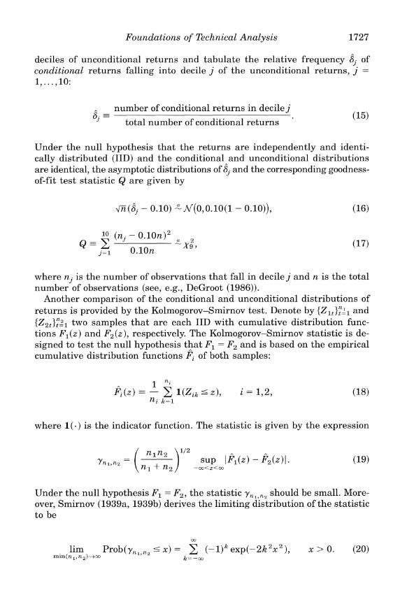

The Journal of Finance
E Summary Statistics
In Tables I and 11 we report frequency counts for the number of patterns detected over the entire 1962 to 1996 sample and within each subperiod and each market-capitalization quintile for the 10 patterns defined in Sec- tion 1IA Table I contains results for the NYSEAMEX stocks and Table I1 contains corresponding results for Nasdaq stocks
Table I shows that the most common patterns across all stocks and over the entire sample period are double tops and bottoms (see the row labeled Entire) with over 2000 occurrences of each The second most common patterns are the head-and-shoulders and inverted head-and-shoulders with over 1600 occurrences of each These total counts correspond roughly to four to six occurrences of each of these patterns for each stock during each five- year subperiod (divide the total number of occurrences by 7 x 50) not an unreasonable frequency from the point of view of professional technical an- alysts Table I shows that most of the 10 patterns are more frequent for larger stocks than for smaller ones and that they are relatively evenly dis- tributed over the five-year subperiods When volume trend is considered jointly with the occurrences of the 10 patterns Table I shows that the fre- quency of patterns is not evenly distributed between increasing (the row labeled r(1)) and decreasing (the row labeled r ( ~ ) ) volume-trend cases For example for the entire sample of stocks over the 1962 to 1996 sample period there are 143 occurrences of a broadening top with decreasing vol- ume trend but 409 occurrences of a broadening top with increasing volume trend
For purposes of comparison Table I also reports frequency counts for the number of patterns detected in a sample of simulated geometric Brownian motion calibrated to match the mean and standard deviation of each stock in each five-year subperiod11 The entries in the row labeled Sim GBM show that the random walk model yields very different implications for the frequency counts of several technical patterns For example the simulated sample has only 577 head-and-shoulders and 578 inverted-head-and- shoulders patterns whereas the actual data have considerably more 1611 and 1654 respectively On the other hand for broadening tops and bottoms the simulated sample contains many more occurrences than the actual data 1227 and 1028 compared to 725 and 748 respectively The number of tri- angles is roughly comparable across the two samples but for rectangles and
l1 In particular le t t h e price process sa t i s fy
where W ( t )i s a standard Brownian motion To generate s imulated prices for a single securi ty i n a g iven period w e es t imate t h e securitys d r i f t and d i f fus ion coef f icients b y m a x i m u m l ike- lihood and t h e n simulate prices us ing t h e est imated parameter values An independent price series i s s imulated for each o f t h e 350 securities i n b o t h t h e NYSEIAR4EX and t h e Nasdaq samples Finally w e u s e our pattern-recognition algori thm t o detect t h e occurrence o f each o f t h e 10 patterns i n t h e s imulated price series
1731 Foundations of Technical Analysis
double tops and bottoms the differences are dramatic Of course the simu- lated sample is only one realization of geometric Brownian motion so it is difficult to draw general conclusions about the relative frequencies Never- theless these simulations point to important differences between the data and IID lognormal returns
To develop further intuition for these patterns Figures 8 and 9 display the cross-sectional and time-series distribution of each of the 10 patterns for the NYSEAMEX and Nasdaq samples respectively Each symbol represents a pattern detected by our algorithm the vertical axis is divided into the five size quintiles the horizontal axis is calendar time and alternating symbols (diamonds and asterisks) represent distinct subperiods These graphs show that the distribution of patterns is not clustered in time or among a subset of securities
Table I1 provides the same frequency counts for Nasdaq stocks and de- spite the fact that we have the same number of stocks in this sample (50 per subperiod over seven subperiods) there are considerably fewer patterns de- tected than in the NYSEAMEX case For example the Nasdaq sample yields only 919 head-and-shoulders patterns whereas the NYSEAMEX sample contains 1611 Not surprisingly the frequency counts for the sample of sim- ulated geometric Brownian motion are similar to those in Table I
Tables I11 and IV report summary statistics-means standard deviations skewness and excess kurtosis-of unconditional and conditional normalized returns of NYSEAMEX and Nasdaq stocks respectively These statistics show considerable variation in the different return populations For exam- ple in Table I11 the first four moments of normalized raw returns are 0000 1000 0345 and 8122 respectively The same four moments of post-BTOP returns are -0005 1035 -1151 and 16701 respectively and those of post-DTOP returns are 0017 0910 0206 and 3386 respectively The dif- ferences in these statistics among the 10 conditional return populations and the differences between the conditional and unconditional return popula- tions suggest that conditioning on the 10 technical indicators does have some effect on the distribution of returns
l Empirical Results
Tables V and VI report the results of the goodness-of-fit test (equations (16) and (17)) for our sample of NYSE and AMEX (Table V) and Nasdaq (Table VI) stocks respectively from 1962 to 1996 for each of the 10 technical patterns Table V shows that in the NYSEAMEX sample the relative fre- quencies of the conditional returns are significantly different from those of the unconditional returns for seven of the 10 patterns considered The three exceptions are the conditional returns from the BBOT TTOP and DBOT patterns for which the p-values of the test statistics Q are 51 percent 212 percent and 166 percent respectively These results yield mixed support for the overall efficacy of technical indicators However the results of Table VI tell a different story there is overwhelming significance for all 10 indicators
-4 I-
Table I W
Frequency counts for 10 technical indicators detected among NYSEAMEX stocks from 1962 to 1996 in five-year subperiods in size quintiles and in a sample of simulated geometric Brownian motion In each five-year subperiod 10 stocks per quintile are selected a t random among stocks with at least 80 nonmissing prices and each stocks price history is scanned for any occurrence of the following 10 technical indicators within the subperiod head-and-shoulders (HS) inverted head-and-shoulders (IHS) broadening top (BTOP) broadening bottom (BBOT) triangle top (TTOP) triangle bottom ITBOT) rectangle top (RTOP) rectangle bottom (RBOT) double top (DTOP) and double bottom (DBOT) The Sample column indicates whether the frequency counts are conditioned on decreasing volume trend (r()) increasing volume trend 1r(1)) uncondi- tional (Entiren) or for a sample of simulated geometric Brownian motion with parameters calibrated to match the data (Sim GBM)
Sample Raw HS IHS BTOP BBOT TTOP TBOT RTOP RBOT UTOP UBOT
All Stocks 1962 to 1996 Entire 748 1294 Sim GBM 1028 1049
~ ( L J 220 666 r(Pi 337 300
Smallest Quintilr 1962 to 1996 Entlre 97 203 Sim GBM 256 269
T ( L ) 42 122
~ ( 7 ) 37 41
2nd Quintile 1962 to 1996 Xntire 150 255 Sim GBM 251 261
7() 48 135 r ( r ) 63 55
3rd Quintile 1962 l o 1996 Entire 161 291 Sim GUM 222 212 r i b ) 49 151 r ( i 66 67
4th Quintile 1962 to 1996 Entire 173 262 Sim GUM 210 183
T ( L ) 42 138 ~ ( 7 1 89 56
Largest Quintile 1962 to 1996 Xntire 167 283 Sim GUM 89 124 T ( L ~ 39 120 7 i P l 82 8 1
Entire Sim GBM
( L ) r()
Entire Sim GBM
T ( L )
r()
Entire Sim GBM
T ( L )
r ( P )
Entlre Sim GRM
T ( L )
r ( P )
Entire Sim GRM
( L ) r ( P )
Entire Slm GRM
T ( L ) ~ ( 3 )
Entire Sim GRM
(I r ( r i
All Stocks 1962 to 1966 103 179 126 129 29 93 39 37
All Stocks 1967 to 1971 134 227 148 150 45 126 57 47
All Stocks 1972 to 1976 93 165
154 156 23 88 50 32
All Stocks 1977 to 1981 110 188 200 188
39 100 44 35
All Stocks 1982 to 1986 108 182 144 152 30 93 62 46
All Stocks 1987 to 1991 98 180
132 131 30 86 43 53
All Stocks 1992 to 1996 102 173 124 143 24 80 42 50
+
Table I1 CS -3
Frequency counts for 10 technical indicators detected among Nasdaq stocks from 1962 to 1996 in five-year subperiods in size quintiles and in a sample of simulated geometric Brownian motion In each five-year subperiod 10 stocks per quintile are selected a t random among stocks with at least 80 nonmissing prices and each stocks price history is scanned for any occurrence of the following 10 technical indicators within the subperiod head-and-shoulders (HS) inverted head-and-shoulders (IHS) broadening top (BTOP) broadening bottom (BBOT) triangle top ITTOP) triangle bottom (TBOT) rectangle top (RTOP) rectangle bottom (RBOT) double top (DTOP) and double bottom (DBOT) The Sample column indicates whether the frequency counts are conditioned on decreasing volume trend (~(h)) unconditionalincreasing volume trend ( ~ ( p ) ) (Entire) or for a sample of simulated geometric Brownian motion with parameters calibrated to match the data (Sirn GBM) - - --- ----- --
Samplc Raw HS IHS RTOP BBOT TTOP TBOT RTOP IZROT DTOP DBOT -- -- -- -- -- - - - - -
All Stocks 1962 to 1996 Entire 411010 919 817 414 508 850 789 1134 1320 1208 1147 Sim GEM 411010 434 447 1297 1139 1169 1309 96 91 567 579 h3 (L) - 408 268 69 133 429 460 488 550 339 580 $ T ( I - 284 325 234 209 185 125 391 461 474 229 q
Smallest Quintile 1962 to 1996 0
Entire 81754 84 64 41 73 111 93 165 218 113 125 3 Sim GBM 81754 85 84 341 289 334 367 11 12 140 125
T ( L gt 36 25 6 20 66 59 77 102 31 81 5-
T ( ) - 31 23 31 30 24 15 59 85 46 2nd Quintile 1962 to 1996 l7
Entire 81336 191 138 68 88 161 148 242 305 219 176 Sim GBM 81336 67 84 243 225 219 229 24 12 99 124 5 ( I - 94 51 11 28 86 109 111 131 69 101 a T() - 66 57 46 38 45 22 85 120 90 42 2
m 3rd Quintile 1962 to 1996
Entirc 81772 224 186 105 121 183 155 235 244 279 267 Sim GBM 81772 69 86 227 210 214 239 15 14 105 100
(L) - 108 66 23 35 87 91 90 84 78 145 T() 7 1 79 56 49 39 29 84 86 122 58-
4th Quintile 1962 to 1996 Entirc 82727 212 214 92 116 187 179 296 303 289 29 7 Sim GBM 82727 104 92 242 219 209 255 23 26 115 97
T ( L ) - 88 68 12 26 101 101 127 141 77 143 T() - 62 83 57 56 34 22 104 Y3 118 66
Idurgest Quintile 1962 to 1996 Entire 83421 208 215 108 110 208 214 196 250 308 282 Sim GHM 83421 109 101 244 196 193 219 23 27 108 133
T(L) - 82 58 17 24 99 100 83 92 84 110 T() - 54 83 44 36 43 37 59 77 98 46
Entire Sim GBM r() ~ ( r )
Entlre Slm GBM r() ~ ( 7 )
Entirc Sim GBM
(I ~ ( 7 )
Entirc Sim GBM
T ( L )
~ ( 1 1 )
Entirc Sim GBM
T ( ) ~ ( 7 )
Entirc Sim GBM
+ L ) ~ ( 7 )
Entirc Sim GBM
(I ~ ( 7 )
All Stocks 1962 to 1966 99 182
123 137 23 104 5 1 37
All Stock 1967 to 1971 123 227 184 181 40 127 51 45
All Stock 1972 to 1976 30 29
113 107 4 5 2 2
A11 Stocks 1977 to 1981 36 52
165 176 2 4 I 4
All Stock 1982 to 1986 44 97
168 147 14 46 18 26
All Stock 1987 to 1991 61 120
187 205 19 73 30 26
All Stock 1992 to 1996 115 143 199 216 31 70 56 45
1736 The Journal of Finance
Date
(a)
Foundations of Technical Analysis
Date
(dl
Figure 8 Continued
The Journal of Finance
Date
(el
Date
(f)
Figure 8 Continued
Foundations of Technical Analysis
RTOP (NYSEIAMEX)
w--+ c-
6
1965 1970 1975 1980 1985 1990 1995 Date
(9)
RTOP (NYSEIAMEX) 5
4
3
w--+ -6
2
1
1965 1970 1975 1980 1985 1990 1995 Date
(h)
Figure 8 Continued
1740 The Jourrzal o f Finarzce
DTOP (NYSUAMEX)
Date
(i)
Date
(1)
Figure 8 Continued
Foundations of Technical Analysis
HS (NASDAQ)
0---c-6
O O 0
1965 1970 1975 1980 Date
(a)
IHS (NASDAQ)
1985 1990 1995
a--+ -6
0 0 0
Y V + ^ 1965 1970 1975 1980 1985 1990 1995
Date
(b)
Figure 9 Distribution of patterns in Nasdaq sample
The Journal of Finance
BTOP (NASDAQ)
O Mi
C 0
Mi
00 0 0
0 0 2 0 0 0 v
00 0
O Ht v v o 0 A 9
C
aoOO O 0 0 0
0
0
0
0 O0
OC 0 O I a
1965 1970 1975 1980 1985 1990 1995 Date
BTOP (NASDAQ) 50 A A h
i V V
V b
O m 0
0 Mi
0 0
00 0 4 - 0 amp 0
O v
0
00 0
O Ht v v o o A 9
v0
C0 0 0 0 0
0
I 0
0
so0 O o 0 Oo
$ 0 OC i v o a
1965 1970 1975 1980 1985 1990 1995 Date
Figure 9 Continued
Foundations of Technical Analysis
Date
(e)
Date
(0 Figure 9 Continued
1744 The Joul-nal of Finance
RTOP (NASDAQ) A A A A
I 0 0 o 3 o o
0
Date
(9)
RBOT (NASDAQ)
a --+ -6
0 00
0 OQO
1965 1970 1975 1980 1985 1990 1995 Date
(h)
Figure 9 Continued
F o ~ ~ n d a t i o n sof Technical Analysis
DTOP (NASDAQ1
Date
0)
Date
(J)
Figure 9 Continued
Table I11 Summary statistics (mean standard deviation skewness and excess kurtosis) of raw and conditional one-day normalized returns of NYSE AMEX stocks from 1962 to 1996 in five-year subperiods and in size quintiles Conditional returns are defined as the daily return three days following the conclusion of an occurrence of one of 10 technical indicators head-and-shoulders (HS) inverted head-and-shoulders (IHS)broad-ening top (BTOP) broadening bottom (BBOT) triangle top (TTOP) triangle bottom (TBOT) rectangle top (RTOI) rectangle bottom (RBOT) double top (DTOP) and double bottom (DBOT) All returns have been normalized by subtraction of their means and division by their standard deviations
~-
Moment Raw NS IIIS BTOP BBOT TTOI TBOT RTOIJ RBOT DTOP IIHOT
All Stocks 1962 to 1996 Mean -0062 0021 SD 0979 0955 Skew 0090 0137 Kurt 3 169 3293
Smallest Quintile 1962 to 1996 Mean -0188 0036 SD 0850 0937 Skew -0367 0861 Kurt 0575 4185
2nd Quintile 1962 to 1996 Mean -0113 0003 SD 1004 0913 Skew 0485 -0529 Kurt 3779 3024
3rd Quintile 1962 to 1996 Mean -0056 0036 SD 0925 0973 Skew 0233 0538 Kurt 0611 2995
4th Quintile 1962 to 1996 Mean 0 028 0022 SD 1093 0986 Skew 0537 -0217 Kurt 2168 4237
Largest Quintrie 1962 to 1996 Mean -0042 0010 SD 0951 0964 Skew -1099 0089 Kurt 6603 2107
Foundations of Technical Analysis
O N ~ N m m - m m m w c m m d o m w c o C N ~ C ~ ~ m m m O C O C - m t - m o m o o m e c m i m d ~ w o d m m m i m r - L C -9q q o q r - m I ~ N N q q c q 2 2 ~ q q m o o o a m O O O i o a o m O i N m 0 - a t - a - a m -I I I I I I I I
i m c m m m o c - + - $ c o o ~ t - i m r i o m m m m d m m o i ce m m i m m w m m i m m d m w m - + L O N - ~ c m o o w m oX $ g z Z Z Z $ 0 0 L D -L
0 0 0 m - C O N 0 0 o i 0 0 0 - I I I I I I
m d - o o m m d m d m c W C O ~m m c d~ o m m m m w m md i m 0 i w m m a m m m ~ m m m o m w m m m m t - d m m m$ Z 0 5 a e m
C O O N o a o d o o o m o o o w I I I I
- r ( ~ r ( i i m w m o e c e m d o o ~ ~ i o d m mm m e t - m m w m w o m m m N C ~ N o m m r - m m m o e m m e m i w o e q c o y o q o t - 9 5 q m q f l 9 ~ 9 q o o i c o o d m o o o m o o o - o o o - o o o i o o o o
1 - I I I I I I
m r t b w c w ~ m O N ~ N o i o m e - m m m - w w - m o mm r i c o ~ m m m m - N C - m i - m w o d c o m - m d r - m m8 3 2 2 O F X$ - 9 0 0 0 deg F
0 0 0 3 0 i 0 0 = = + L C 0 0 - 0 O ~ N N I I I I I
m m m r - m m d ~ ~ i m m w - m m c i w m- m m ~ w m m i ~ m ~ w m m a 0 0 o m m w t - i m w d o t - m m m o a m o m m - o q m q 0 7 9 ~ 0 0 a f l c o 0 9 f l m y d q q o o a o a 0 0 0 0 o o c o o i i d 0 - O N o o o ~ o i m t -
I I I I I N
o c m ~ d m b d m m e w m w e m m m d a c m w m e m m mt - m m i m o m m m i m m m m m m m m m m m e d m m m e m9 y - w o o m q i c m - 9 m q o q q m q ~ q q 0 0 0 0 0 0 0 m o - o m o o o i o o o ~ o o o m o o o m
I I I I I I I I I
o o m i o o m o o o m o o o w m o o o m o o m m o o m m0 0 ~ 0 w o o m i 0 0 - N o o m r ( o a m m 0 o - t - o o o m
XS$S= $ 2 2 2 X z g z 922I I I I I I 1 - I
Table IV Summary statistics (mean standard deviation skewness and excess kurtosis) of raw and conditional one-day normalized returns of Nasdaq stocks from 1962 to 1996 in five-year subperiods and in size quintiles Conditional returns are defined as the daily return three days following the conclusion of an occurrence of one of 10 technical indicators head-and-shouldttrs (HS) inverted head-and-shoulders (II-IS) broadening top (BTOP) broadening bottom (RROT) triangle top (TTOP) triangle bottom (TBOT) rectangle top (ItTOP) rectangle bottom (RBOT) double top (DTOP) and double bottom (DBOT) All returns have been normalized by subtraction oftheir means and division by their standard deviations
Moment Raw HS IHS BTOI
Mean SD Skew Kurt
Mean SD Skew Kurt
Mean SD Skew Kurt
Mean SD Skevi Kurt
Mean SD Skew Kurt
Mean SD Skew Kurt
BBOT TTOI TBOT RTOI RBOT DTOP DBOT
All Stocks 1962 to 1996 0009 -0020 0995 0984 0 586 0895 2783 6692
Smallest Quintile 1962 to 1996 - 0153 0069
0894 1113 -0109 2 727 0571 14270
2nd Quintile 1962 to 1996 -0093 0 0 8 5
1026 0805 0636 0036 I458 0689
3rd Quintrlr 1962 to 1996 0210 - 0030 0971 0825 0326 0639 0430 1673
4th Quintile 1962 to 1996 - 0044 0 0 8 0
0975 1076 0385 0554 1601 7723
Largcst Quintile 1962 to 1996 0031 0 052 1060 1076 1225 0409 0778 1970
Foundations of Technical Analysis
- 0 - m m a m m o m 0 0 0 0
w 3 - m o m m e q q v q0 0 3 0
m v - o c m m -- i o 7 0 0 0 0 0
o o - N x r m e m o w q w0 100
N N - mi n m e -o c c w 3 - 3 3
~ o m ~ m c - m m 0 0 3 N
m m a c e =
~ w o 0 0 3 3
q
I I I I I I I I I I
m m m c O N L Q L Q v v - a i m o c a m - + m m m m m m m m m m m c o m m m o ~ m m m m m ~ ~ w o c a c o - o m m m o c q q o m y ~ o m o q 9 - q m c - 0 7 1 c q o ~ O - O a O O I I 3 0 7 3 3 I I 0 3 0 - 10 3 0 0 0 3 0
o m - m w m m m I C N O m i m i o w o q - 1 0 0 90 0 - m O - - L r
3 m w m v m o m3 0 1 3 ~ 9 m i - -e q q w - o w o o ~ m o - a -
m m m o - m a = m m m m ~ m c o m 0 q d 9 0 0 0 0 0 3 3 0
- m x r ~ ~ x r ~ o a m a m - = m ac7- w e 0 3 - 0 0 3 - N
O O ~ L Q a a v v3 3 ~ ~ 3 0 m m9 3 3 m m c q y - 3 - 3 w 0 - o m I I
m o c o C C - r i w a m v o - x r - c a c w - m a -- m 0 9 - o ~ q - w q y0 0 0 m 0 - 0 0 3 3 3 3
w w m a ~ ( o - c m o o = C ~ N N m m m m N - m m q m y m o c - 1 q m - 7O O N W o - m e 0 3 3 3 I - I I
m m m c ~ i - w c a - m m o m c c i m m w m a o m
d m - o - 0 c 7 - q a m 3 0 - 0 = - a m o o o o
I I 1 1
m m m m ~ m w c a m m a m o c m - ~ - e a v m m -- 1 i-ii
1 I
o o m m 3 0 ~ m a o c m o o m m = = m a o o m m o c v q 3 coo 0 3 C o - o e O h - 0 O d d -
- 1 N 0
m o m o - m w m l x r o ~ m q o c mO i O N
m w m m w m m m m m m m c m q c o o a -
3 m ~ m m ~ a m 3 e m w 0 0 3 -I I
o w m m m x r t n e ~ m c m m m - m 2 2 - Z z - Z i
1 1 1
--
CL
Table V ul-4
0Goodness-of-fit diagnostics for the conditional one-day normalized returns conditional on 10 technical indicators for a sample of 350 NYSEIAMEX stocks from 1962 to 1996 (10 stocks per size-quintile with a t least 80 nonmissing prices are randomly chosen in each five-year subperiod yielding 50 stocks per subperiod over seven subperiods) For each pattern the percentage of conditional returns that falls within each of the 10 unconditional-return deciles is tabulated If conditioning on the pattern provides no information the expected percentage falling in each decile is 10Asymptotic z-statistics for this null hypothesis are reported in parentheses and the X goodness-of-fitness test statistic Q is reported in the last column with the p-value in parentheses below the statistic The 10 technical indicators are as follows head-and-shoulders (HS) inverted head-and-shoulders (IHS) broadening top (BTOP) broadening bottom (BBOT) triangle top (TTOP) triangle bottom (TBOT) rectangle top (RTOP) rectangle bottom (RBOT) double top (DTOP) and double bottom (DBOT)
Decile - Q YPattern 1 2 3 4 5 6 7 8 9 10 (p-Value) 2-
HS 89 104 112 117 122 79 92 104 108 71 3931 3 (-149) (056) (149) (216) (273) (-305) (-104) (048) (104) (-446) (0000) s
IHS 86 97 94 112 137 77 91 111 96 100 4095 2 (-205) (-036) (-088) (160) (434) (-344) (-132) (138) (-062) (-003) (0000)
BTOP 94 106 106 119 87 66 92 137 92 101 2340 (-057) (054) (054) (155) (-125) (-366) (-071) (287) (-071) (006) (0005) 3
BBOT 115 99 130 111 78 92 83 90 107 96 1687 2 (128) (-010) (242) (095) (-230) (-073) (-170) (-100) (062) (-035) (0051) $
TTOP 78 104 109 113 90 99 100 107 105 97 1203 c3m (-294) (042) (103) (146) (-130) (-013) (-004) (077) (060) (-041) (0212)
TBOT 89 106 109 122 92 87 93 116 87 98 1712 (-135) (072) (099) (236) (-093) (-157) (-083) (169) (-157) (-022) (0047)
RTOP 84 99 92 105 125 101 100 100 114 81 2272 (-227) (-010) - 1 1 ) (058) (289) (016) (-002) (-002) (170) (-269) (0007)
RBOT 86 96 78 105 129 108 116 93 103 87 3394 (-201) (-056) (-330) (060) (345) (107) (198) (-099) (044) (-191) (0000)
DTOP 82 109 96 124 118 75 82 113 103 97 5097 (-292) (136) (-064) (329) (261) (-439) (-292) (183) (046) (-041) (0000)
DBOT 97 99 100 109 114 85 92 100 107 98 1292 (-048) (-018) (-004) (137) (197) (-240) (-133) (004) (096) (-033) (0166)
-
lable VI
Goodness-of-fit diagnostics for the conditional one-day normalized returns conditional on 10 technical indicators for a sample of 350 Nasdaq stocks from 1962 to 1996 (10 stocks per size-quintile with a t least 80 nonmissing prices are randomly chosen in each five-year subperiod yielding 50 stocks per subperiod over seven subperiods) For each pattern the percentage of conditional returns that falls within each of the 10 unconditional-return deciles is tabulated If conditioning on the pattern provides no information the expected percentage falling in each decile is 10Asymptotic z-statistics for this null hypothesis are reported in parentheses and the y2 goodness-of-fitness test statistic Q is reported in the last column with the p-value in parentheses below the statistic The 10 technical indicators are as follows head-and-shoulders (HS) inverted head-and-shoulders (IHS) broadening top (BTOP) broadening bottom (BBOT) triangle top (TTOP) triangle bottom (TBOT) rectangle top (RTOP) rectangle bottom (RBOT) double top (DTOP) and double bottom (DBOT)
2 Decile 2
F - - --- Q
Pattern 1 2 3 4 5 6 7 8 9 10 (p-Value) 8- --- -- 6
HS 108 108 137 86 85 60 60 125 135 97 6441 2 (076) (076) (327) (-152) (-165) (-513) (-513) (230) (310) (-032) (0000)
IHS 94 141 125 80 77 48 64 135 125 113 7584 (-056) (335) (215) ( -216) (-245) (-701) (-426) (290) (215) (114) (0000)
BTOP 116 123 128 77 82 68 43 133 121 109 3412 3
(101) (144) (171) (-173) (-132) (-262) (-564) (197) (130) (057) (0000) $ BBOT 114 114 148 59 67 96 57 114 98 132 4326 R
(100) (100) (303) (-391) (-298) (-027) (--417) (100) (-012) (212) (0000) L+
TTOP 107 121 162 62 79 87 40 125 114 102 9209 2 (067) (189) (493) (-454) (-229) (-134) (-893) (218) (129) (023) (0000)
TBOT 99 113 156 79 77 57 53 146 120 100 8526 (-011) (114) (433) (-224) (-239) (-520) (-585) (364) (176) (001) (0000)
RTOP 112 108 88 83 102 71 77 93 153 113 5708 (128) (092) (-140) (-209) (025) (-387) (-295) (-075) (492) (137) (0000)
RBOT 89 123 89 89 116 89 70 95 136 103 4579 (-135) (252) (-135) (-145) (181) (-135) (-419) (-066) (385) (036) (0000)
DTOP 110 126 117 90 92 55 58 116 123 113 7129 (112) (271) (181) (-118) (-098) (-676) (-626) (173) (239) (147) (0000)
DBOT 109 115 131 80 81 71 76 115 128 93 5123 (098) (160) (309) (-247) (-235) (-375) (-309) (160) (285) (-078) (0000) 5
-- a - -- - - U7
li
1752 The Journal of Finance
in the Nasdaq sample with p-values that are zero to three significant digits and test statistics Q that range from 3412 to 9209 In contrast the test statistics in Table V range from 1203 to 5097
One possible explanation for the difference between the NYSEAMEX and Nasdaq samples is a difference in the power of the test because of different sample sizes If the NYSEAMEX sample contained fewer conditional re- turns that is fewer patterns the corresponding test statistics might be sub- ject to greater sampling variation and lower power However this explanation can be ruled out from the frequency counts of Tables I and 11-the number of patterns in the NYSEAMEX sample is considerably larger than those of the Nasdaq sample for all 10 patterns Tables V and VI seem to suggest important differences in the informativeness of technical indicators for NYSE AMEX and Nasdaq stocks
Table VII and VIII report the results of the Kolmogorov-Smirnov test (equa- tion (19)) of the equality of the conditional and unconditional return distri- butions for NYSEAMEX (Table VII) and Nasdaq (Table VIII) stocks respectively from 1962 to 1996 in five-year subperiods and in market- capitalization quintiles Recall that conditional returns are defined as the one-day return starting three days following the conclusion of an occurrence of a pattern The p-values are with respect to the asymptotic distribution of the Kolmogorov-Smirnov test statistic given in equation (20) Table VII shows that for NYSEAMEX stocks five of the 10 patterns-HS BBOT RTOP RBOT and DTOP-yield statistically significant test statistics withp-values ranging from 0000 for RBOT to 0021 for DTOP patterns However for the other five patterns thep-values range from 0104 for IHS to 0393 for TTOP which implies an inability to distinguish between the conditional and un- conditional distributions of normalized returns
When we also condition on declining volume trend the statistical signif- icance declines for most patterns but the statistical significance of TBOT patterns increases In contrast conditioning on increasing volume trend yields an increase in the statistical significance of BTOP patterns This difference may suggest an important role for volume trend in TBOT and BTOP pat- terns The difference between the increasing and decreasing volume-trend conditional distributions is statistically insignificant for almost all the pat- terns (the sole exception is the TBOT pattern) This drop in statistical sig- nificance may be due to a lack of power of the Kolmogorov-Smirnov test given the relatively small sample sizes of these conditional returns (see Table I for frequency counts)
Table VIII reports corresponding results for the Nasdaq sample and as in Table VI in contrast to the NYSEAMEX results here all the patterns are statistically significant a t the 5 percent level This is especially significant because the the Nasdaq sample exhibits far fewer patterns than the NYSE AMEX sample (see Tables I and 11) and hence the Kolmogorov-Smirnov test is likely to have lower power in this case
As with the NYSEAMEX sample volume trend seems to provide little incremental information for the Nasdaq sample except in one case increas- ing volume and BTOP And except for the TTOP pattern the Kolmogorov-
1753 Foundations of Technical Analysis
Smirnov test still cannot distinguish between the decreasing and in- creasing volume-trend conditional distributions as the last pair of rows of Table VII17s first panel indicates
IV Monte Carlo Analysis
Tables IX and X contain bootstrap percentiles for the Kolmogorov- Smirnov test of the equality of conditional and unconditional one-day return distributions for NYSEAMEX and Nasdaq stocks respectively from 1962 to 1996 for five-year subperiods and for market-capitalization quintiles un- der the null hypothesis of equality For each of the two sets of market data two sample sizes m and m have been chosen to span the range of fre- quency counts of patterns reported in Tables I and 11 For each sample size m we resample one-day normalized returns (with replacement) to obtain a bootstrap sample of m observations compute the Kolmogorov-Smirnov test statistic (against the entire sample of one-day normalized returns) and re- peat this procedure 1000 times The percentiles of the asymptotic distribu- tion are also reported for comparison in the cblumn labeled A
Tables IX and X show that for a broad range of sample sizes and across size quintiles subperiod and exchanges the bootstrap distribution of the Kolmogorov-Smirnov statistic is well approximated by its asymptotic distri- bution equation (20)
V Conclusion
In this paper we have proposed a new approach to evaluating the efficacy of technical analysis Based on smoothing techniques such as nonparametric kernel regression our approach incorporates the essence of technical analy- sis to identify regularities in the time series of prices by extracting nonlin- ear patterns from noisy data Although human judgment is still superior to most computational algorithms in the area of visual pattern recognition recent advances in statistical learning theory have had successful applica- tions in fingerprint identification handwriting analysis and face recogni- tion Technical analysis may well be the next frontier for such methods
We find that certain technical patterns when applied to many stocks over many time periods do provide incremental information especially for Nas- daq stocks Although this does not necessarily imply that technical analysis can be used to generate excess trading profits it does raise the possibility that technical analysis can add value to the investment process
Moreover our methods suggest that technical analysis can be improved by using automated algorithms such as ours and that traditional patterns such as head-and-shoulders and rectangles although sometimes effective need not be optimal In particular it may be possible to determine optimal pat- terns for detecting certain types of phenomena in financial time series for example an optimal shape for detecting stochastic volatility or changes in regime Moreover patterns that are optimal for detecting statistical anom- alies need not be optimal for trading profits and vice versa Such consider-
t-L -2Table VII Crc
Kolmogorov-Smirnov test of the equality of conditional and unconditional one-day return distributions for NYSEIAMEX stocks from 1962 to iP
1996 in five-year subperiods and in size quintiles Conditional returns are defined as the daily return three days following the conclusion of an occurrence of one of 10 technical indicators head-and-shoulders (HS) inverted head-and-shoulders (IHS) broadening top (BTOP) broadening bottom (RROT) triangle top (TTOP) triangle bottom (TBOT) rectangle top IRTOP) rectangle bottom (RBOT) double top (DTOP) and double bottom (DBOT) All returns have been normalized by subtraction of their means and division by their standard deviations p-values are with respect to the asymptotic distribution of the Kolmogorov-Smirnov test statistic The syinbols T() and ~ ( 7 ) indicate that the conditional distribution is also conditioned on decreasing and increasing volume trend respectively
Stat is t~c HS 11-1S RTOP HBOT TTOP TROT RTOP RBOT DTOP DROT
All Stocks 1962 to 1996 Y 176 090 109 p-value 0004 0393 0185 Y T(L) 062 073 133 p-value 0839 0657 0059 r r ( j l 159 092 129 p-value 0013 0368 0073 y Diff 094 075 137 p-value 0342 0628 0046
Smallest Quintile 1962 to 1996 Y 120 098 143 p-value 0114 0290 0033 y ( ) 069 100 146 p-Vdl~10 0723 0271 0029 y 7 i 7 ) 103 047 088 p-value 0236 0981 0423 y Diff 068 048 098 p-value 0741 0976 0291
2nd Quintile 1962 to 1996 Y 092 082 084 p value 0365 0505 0485 Y 7(J 042 091 090 p-value 0994 0378 0394 7 7 i J 083 089 098 p-value 0497 0407 0289 y [)Iff 071 122 092 p value 0687 0102 0361
r p-value r T L ) p-value r T ( P ) p-value y Diff p-value
Y p-value Y T ( L ) p-value Y T ( P ) p-value y 1)iff p-value
r p-value
r T ( L ) p-value r ~ ( 7 ) p-value y Uiff p -value
Y p-value r T ( L ) p-value r ~ ( 7 ) p-value y Diff p-value
3rd Quintile 1962 to 1996 128 057 103 0074 0903 0243 076 061 082 0613 0854 0520 114 063 080 0147 0826 0544 048 050 089 0974 0964 0413
4th Quintile 1962 to 1996 084 061 084 0479 0855 0480 096 078 084 0311 0585 0487 096 116 069 0316 0137 0731 116 131 078 0138 0065 0571
Largest Quintile 1962 to 1996 048 0977 078 0580 061 0854 064 0800
072 0671 080 0539 084 0475 076
050 0964 064 0806 069 0729 076 0607
All Stocks 1962 to 1966 075 0634 063 0826 058 0894 060
0615 0863
080 0544 117 0127 081 0532 121 0110
132 0062 180 0003 140 0040 190 0001
continued r 4ul CT(
Y p-value
Y T ( L ) p-value
Y ~ ( 7 ) p-value y Diff p-value
Y p-value
Y T()
p-value
Y ~ (7) p-value y Diff p-value
Y p-value
Y T ( L ) p-value
Y ~ ( 7 ) p-value y Diff p-value
146 0029 130 0070 062 0831 081 0532
067 0756 072 0673 137 0046 106 0215
189 0002 089 0404 142 0036 049 0971
All Stocks 1982 to 1986 147 104 0027 0232 153 121 0018 0106 083 123 0499 0097 074 121 0643 0107
All Stocks 1987 to 1991 075 086 0627 0456 103 081 0235 0522 074 110 0639 0181 067 093 0753 0357
All Stocks 1992 to 1996 127 094 0078 0343 111 103 0174 0242 102 058 0246 0895 043 081 0993 0528
P -4Table VIII 01
Kolmogorov--Smirnov test of the equality of conditional and unconditional one-day return distributions for Nasdaq stocks from 1962 to 1996 in 03
five-year subperiods and in size quintiles Conditional returns are defined as the daily return three days following the conclusion of an occur- rence of one of 10 technical indicators head-and-shoulders (HS) inverted head-and-shoulders (IHS) broadening top (BTOP) broadening bottom (BBOT) triangle top (TTOP) triangle bottom (TBOT) rectangle top (RTOP) rectangle bottom (RBOT) double top (DTOP) and double bottom (DBOT) All returns have been normalized by subtraction of their means and division by their standard deviations p-values are with respect to the asymptotic distribution of the Kolmogorov-Smirnov test statistic The symbols r() and ~(7)indicate that the conditional distribution is also conditioned on decreasing and increasing volume trend respectively
Statistic HS IHS BTOP BBOT TTOP TROT RTOP RROT DTOP DBOT
All Stocks 1962 to 1996 Y 184 281 234 p-value 0002 0000 0000 Y 7( ) 099 197 195 p-value 0281 0001 0001 Y ~ ( 7 ) 159 189 118 p-value 0013 0002 0126 y Diff 080 173 074 p-value 0542 0005 0637
Smallest Quintile 1962 to 1996 Y 168 122 155 p-value 0007 0101 0016 Y 7 ( ) 114 125 162 p-value 0150 0089 0010 Y (7) 200 134 079 p-value 0001 0055 0553 y Diff 144 139 078 p-value 0031 0042 0574
2nd Quintile 1962 to 1996 Y 144 124 108 p-value 0031 0095 0192 Y 7( ) 092 123 079 p-value 0371 0097 0557 Y ~ ( 7 ) 097 138 129 p-value 0309 0044 0073 y Diff 069 102 105 p-value 0733 0248 0224
Y p-value Y T ( L ) p-value Y T ( P ) p-value y DiE p-value
Y p-value
Y T ( L ) p-value Y d) p-value y Diff p-value
Y p-value Y T ( L ) p-value Y ~ ( 2 ) p-value y Diff p-value
Y p-value
Y T ( L ) p-value Y T ( P ) p-value y Diff p-value
3rd Quintile 1962 to 1996 171 141 152 0006 0038 0020 123 106 102 0097 0213 0245 137 075 101 0047 0633 0262 046 061 089 0984 0844 0404
4th Quirrtile 1962 to 1996 098 130 125 0298 0067 0087 105 092 106 0217 0367 0215 053 225 071 0938 0000 0696 097 186 062 0301 0002 0843
Largest Quintile 1962 to 1996 066 092 068 0778 0360 0742 047 077 076 0981 0587 0612 093 088 125 0358 0415 0089 084 076 111 0476 0617 0169
All Stocks 1962 to 1966 082 071 070 0508 0697 0718 105 051 113 0224 0956 0155 073 135 049 0663 0052 0972 069 129 058 0735 0071 0892
Table VIII-Continuecl -
Statistic IHS BTOP -
BBOT TTOP TBOT RTOP RBOT DTOP DBOT -
Y p-value
Y 7 ( ) p-value Y 7( 1) p-value y Diff p-value
100 0273 070 0714 112 0165 066 0770
All Stocks 1967 to 1971 074 127 0637 0079 087 124 0438 0092 064 079 0810 0566 078 107 0585 0203
074 0642 083 0490 053 0941 040 0997
121 0107 145 0031 069 0723 076 0602
Y 184 All Stocks 1972 to 1976
113 145 096 176 p-value Y r ( ) p-value Y r(1) p-value y Diff
0002 9900
0000 -9900
0000 - 9900
0156 091 0376
-9900 0000
9900 ---
0029 139 0042
9 9 0 0 0000
9 9 0 0
0314 098 0292 076 0611 055
0004 094 0344 065 0798 037
p-value 0000 0000 0000 0925 0999
Y p-value
Y 7 ( ) p-value
103 0236
9 9 0 0 0000
All Stocks 1977 to 1981 102 155 0249 0016
-9900 096 0000 0317
062 0842 079 0554
128 0077 068 0748
Y ~ ( 2 ) p-value y Diff p-value
080 0542
9 9 0 0 0000
99 00 0000
- 9900 0000
146 0028 035 1000
082 0514 037 0999
094 0336 053 0944
y$
35 3R h
53
122
Y p-value Y T ( L ) p-value Y ~(7) p-value y Diff p-value
Y p-value
Y T() p-value Y d ) p-value y Diff p-value
Y p-value Y T() p-value Y ~(7) p-value y Diff p-value
073 0654 074 0641 042 0995 042 0994
088 0421 078 0580 132 0060 128 0075
090 0394 078 0578 100 0275 062 0840
All Stocks 1982 t o 1986 146 169 0028 0006 095 147 0330 0027 117 104 0129 0231 085 043 0462 0993
All Stocks 1987 t o 1991 128 141 0074 0039 168 092 0007 0369 065 127 0787 0078 122 092 0102 0360
All Stocks 1992 to 1996 097 091 0299 0379 081 093 0532 0357 110 104 0180 0231 115 114 0139 0148
The Journal of Finance
Table M Bootstrap percentiles for the Kolmogorov-Smirnov test of the equality of conditional and un- conditional one-day return distributions for NYSEAMEX and Nasdaq stocks from 1962 to 1996 and for size quintiles under the null hypothesis of equality For each of the two sets of market data two sample sizes lnl and 1n2 have been chosen to span the range of frequency counts of patterns reported in Table I For each sample size m we resample one-day normal- ized returns (with replacement) to obtain a bootstrap sample of m observations compute the Kolmogorov-Smirnov test statistic (against the entire sample of one-day normalized returns) and repeat this procedure 1000 times The percentiles of the asymptotic distribution are also reported for comparison
NYSEAMEX Sample Nasdaq Sample -
Percent~le r r ~ A 117 1gt 1 m I A rr12 A gt
All Stocks 1962 to 1996 725 0435 0441 1320 725 0535 0520 1320 725 0590 0571 1320 725 0836 0828 1320 725 1237 1224 1320 725 1395 1358 1320 725 1611 1628 1320
Smallest Quintile 1962 to 1996 78 0406 0441 218 78 0502 0520 218 78 0559 0571 218 78 0814 0828 218 78 1204 1224 218 78 1330 1358 218 78 1590 1628 218
2nd Quintile 1962 to 1996 146 0428 0441 305 146 0505 0520 305 146 0553 0571 305 146 0823 0828 305 146 1210 1224 305 146 1343 1358 305 146 1626 1628 305
3rd Quintile 1962 to 1996 145 0458 0441 279 145 0508 0520 279 145 0557 0571 279 145 0835 0828 279 145 1251 1224 279 145 1397 1358 279 145 1661 1628 279
4th Quintile 1962 to 1996 173 0418 0441 303 173 0516 0520 303 173 0559 0571 303 173 0815 0828 303 173 1183 1224 303 173 1313 1358 303 173 1592 1628 303
Largest Quintile 1962 to 1996 167 0425 0441 308 167 0500 0520 308 167 0554 0571 308 167 0817 0828 308 167 1202 1224 308 167 1308 1358 308 167 1615 1628 308
1
Foundations of Technical Analysis
Table X Bootstrap percentiles for the Koln~ogorov-Smirnov test of the equality of conditional and un- conditional one-day return distributions for NYSEIAMEX and Nasdaq stocks from 1962 to 1996 for five-year subperiods under the null hypothesis of equality For each of the two sets of market data two sample sizes m1 and in have been chosen to span the range of frequency counts of patterns reported in Table I For each sample size in we resample one-day normal- ized returns (with replacement) to obtain a bootstrap sample of m observations conlpute the Kolmogorov-Smirnov test statistic (against the entire sample of one-day normalized returns) and repeat this procedure 1000 times The percentiles of the asymptotic distribution are also reported for conlparison
NYSEAMEX Sample Nasdaq Sample
Percentile A n22 A A 7711 A 7122 A
All Stocks 1962 to 1966 0431 85 0427 0441 342 0460 72 0417 0516 85 0509 0520 342 0539 72 0501 0576 85 0559 0571 342 0589 72 0565 0827 85 0813 0828 342 0849 72 0802 1233 85 1221 1224 342 1242 72 1192 1359 85 1363 1358 342 1384 72 1339 1635 85 1711 1628 342 1582 72 1684
All Stocks 1967 to 1971 0432 112 0423 0441 227 0435 65 0424 0522 112 0508 0520 227 0512 65 0498 0588 112 0562 0571 227 0571 65 0546 0841 112 0819 0828 227 0 811 65 0812 1194 112 1253 1224 227 1179 65 1219 1315 112 1385 1358 227 1346 65 1357 1703 112 1563 1628 227 1625 65 1669
All Stocks 1972 to 1976 0439 82 0440 0441 58 0433 25 0405 0518 82 0503 0520 58 0495 25 0479 0588 82 0554 0571 58 0542 25 0526 0854 82 0798 0828 58 0793 25 0783 1249 82 1208 1224 58 1168 25 1203 1406 82 1364 1358 58 1272 25 1345 1685 82 1635 1628 58 1618 25 1616
All Stocks 1977 to 1981 0426 110 0435 0441 96 0430 36 0417 0519 110 0504 0520 96 0504 36 0485 0573 110 0 555 0571 96 0570 36 0542 0841 110 0793 0828 96 0821 36 0810 1262 110 1184 1224 96 1197 36 1201 1383 110 1342 1358 96 1352 36 1371 1598 110 1645 1628 96 1540 36 1545
All Stocks 1982 to 1986 0462 106 0437 0 441 120 0448 44 0417 0542 106 0506 0520 120 0514 44 0499 0585 106 0559 0571 120 0 579 44 0555 0844 106 0819 0828 120 0825 44 0802 1266 106 1220 1224 120 1253 44 1197 1397 106 1369 1358 120 1366 44 1 3 3 7 1727 106 1615 1628 120 1692 44 1631
All Stocks 1987 to 1991 0443 98 0449 0441 312 0455 50 0432 0 513 98 0522 0520 312 0542 50 0517 0565 98 0 566 0571 312 0610 50 0563 0837 98 0813 0828 312 0878 50 0814 1200 98 1217 1224 312 1319 50 1216 1336 98 1 3 4 8 1358 312 1457 50 1323 1626 98 1563 1628 312 1701 50 1648
All Stock 1992 to 1996 0438 102 0432 0441 361 0447 87 0428 0522 102 0506 0 520 361 0518 87 0492 0567 102 0558 0571 361 0559 87 0 550 0824 102 0 818 0828 361 0817 87 0 799 1220 102 1213 1224 361 1226 87 1216 1 3 2 1 102 1310 1358 361 1353 87 1341 1680 102 1616 1628 361 1617 87 1572
The Journal of Finance
ations may lead to an entirely new branch of technical analysis one based on selecting pattern-recognition algorithms to optimize specific objective func- tions We hope to explore these issues more fully in future research
REFERENCES
Allen Franklin and Risto Karjalainen 1999 Using genetic algorithms to find technical trad- ing rules Journal of Financial Economics 51 245-271
Beymer David and Tomaso Poggio 1996 Inlage representation for visual learning Science 272 1905-1909
Blun~e Lawrence David Easley and Maureen OHara 1994 Market statistics and technical analysis The role of volume Journal of Finance 49 153-181
Brock William Joseph Lakonishok and Blake LeBaron 1992 Simple technical trading rules and the stochastic properties of stock returns Journal of Finance 47 1731-1764
Brown David and Robert Jennings 1989 On technical analysis Review of Firzarzcial Studies 2 527-551
Campbell John Andrew W Lo and A Craig MacKinlay 1997 The Econometrics of Financial Markets (Princeton University Press Princeton NJ)
Chan Louis Narasimhan Jegadeesh and Joseph Lakonishok 1996 Monlentum strategies Journal of Finance 51 1681-1713
Chang Kevin and Carol Osler 1994 Evaluating chart-based technical analysis The head-and- shoulders pattern in foreign exchange markets Working paper Federal Reserve Bank of New York
Csaki E 1984 Empirical distribution function in P Krishnaiah and P Sen eds Handbook of Statistics Vol 4 (Elsevier Science Publishers Amsterdam the Netherlands)
DeGroot Morris 1986 Probability and Statistics (Addison Wesley Reading Mass) Edwards Robert and John Magee 1966 Technical Analysis of Stock Trends 5th ed (John
Magee Boston Mass) Grundy Bruce and S Martin 1998 Understanding the nature of the risks and the source of
the rewards to momentum investing Working paper Wharton School University of Pennsylvania
Hardle Wolfgang 1990 Applied Nonparametric Regression (Cambridge University Press Cam- bridge UK)
Hollander Myles and Douglas Wolfe 1973 Nonparametric Statistical Methods (John Wiley amp Sons New York)
Jegadeesh Narasimhan and Sheridan Titman 1993 Returns to buying winners and selling losers Inlplications for stock market efficiency Journal of Finance 48 65-91
Lo Andrew W and A Craig MacKinlay 1988 Stock market prices do not follow random walks Evidence from a simple specification test Review of Finarzcial Studies 1 41-66
Lo Andrew W and A Craig MacKinlay 1997 Maximizing predictability in the stock and bond markets Macroeconomic Dynamics 1 102-134
Lo Andrew W and A Craig MacKinlay 1999 A Non-Random Walk down Wall Street (Prince-ton University Press Princeton NJ)
Malkiel Burton 1996 A Random Walk down Wall Street Includiizg a Life-Cycle Guide to Per- sonal Investing (W W Norton New York)
Neely Christopher Peter Weller and Robert Dittmar 1997 Is technical analysis in the foreign exchange market profitable A genetic programming approach Journal of Firzancial and Quantitative Analysis 32 405-426
Neely Christopher and Peter Weller 1998 Technical trading rules in the European monetary system Working paper Federal Bank of St Louis
Neftci Salih 1991 Naive trading rules in financial markets and Wiener-Kolmogorov predic- tion theory A study of technical analysis Journal of Business 64 549-571
Neftci Salih and Andrew Policano 1984 Can chartists outperform the market Market effi- ciency tests for technical analyst Journal of Future Markets 4 465-478
1765 Foundations of Technical Analysis
Osler Carol and Kevin Chang 1995 Head and shoulders Not just a flaky pattern Staff Re- port No 4 Federal Reserve Bank of New York
Poggio Tomaso and David Beymer 1996 Regularization networks for visual learning in Shree Nayar and Tomaso Poggio eds Early Visual Learning (Oxford University Press Oxford UK)
Press William Brian Flannery Saul Teukolsky and William Vetterling 1986 Numerical Kec- ipes The Art of Scientific Computing (Cambridge University Press Cambridge UK)
Pruitt Stephen and Robert White 1988 The CRISMA trading system Who says technical analysis cant beat the market Journal of Po~tfolio Management 14 55-58
Riesenhuber ~Maximilian and Tomaso Poggio 1997 Common computational strategies in ma- chine and biological vision in Proccedings of International Symposium on System Life (To-kyo Japan) 67-75
Rouwenhorst Geert 1998 International momentum strategies eJou~nalof Finance 53 267-284 Sirnonoff Jeffrey 1996 Smoothing Methods i n Statistics (Springer-Verlag New lTork) Smirnov N 1939a Sur les ecarts de la courbe de distribution empirique Rec Math (Mat
Sborn) 6 3-26 Smirnov N 1939b On the estimation of the discrepancy between empirical curves of distri-
bution for two independent samples Bulletin Math Univ Moscow 2 3-14 Tabell Anthony and Edward Tabell 1964 The case for technical analysis Financial Analyst
eJou~nal20 67-76 Treynor Jack and Robert Ferguson 1985 In defense of technical analysis Journal of Finance
40 757-773
Discussion
NARASIMHAN JEGADEESHK
Academics have long been skeptical about the usefulness of technical trad- ing strategies The literature that evaluates the performance of such trading strategies has found mixed results This literature has generally focused on evaluating simple technical trading rules such as filter rules and moving average rules that are fairly straightforward to define and implement Lo Mamaysky and Wang (hereafter LMW) move this literature forward by eval- uating more complicated trading strategies used by chartists that are hard to define and implement objectively
Broadly the primary objectives of LMW are to automate the process of identifying patterns in stock prices and evaluate the usefulness of trading strategies based on various patterns They start with quantitative defini- tions of 10 patterns that are commonly used by chartists They then smooth the price data using kernel regressions They identify various patterns in the smoothed prices based on their definitions of these patterns Their al- gorithms allow them to recognize patterns objectively on the computer rather
University of Illinois a t Urbana-Champaign
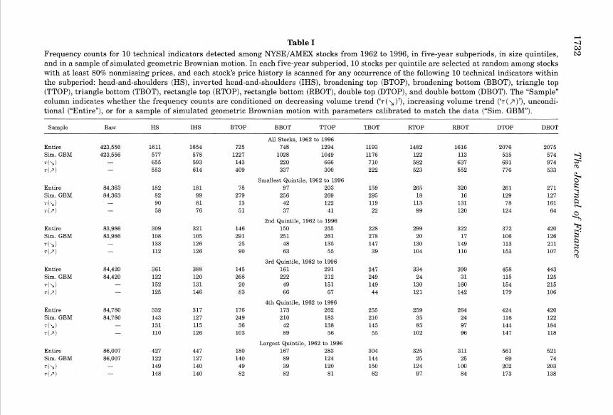

Entire Sim GBM
( L ) r()
Entire Sim GBM
T ( L )
r()
Entire Sim GBM
T ( L )
r ( P )
Entlre Sim GRM
T ( L )
r ( P )
Entire Sim GRM
( L ) r ( P )
Entire Slm GRM
T ( L ) ~ ( 3 )
Entire Sim GRM
(I r ( r i
All Stocks 1962 to 1966 103 179 126 129 29 93 39 37
All Stocks 1967 to 1971 134 227 148 150 45 126 57 47
All Stocks 1972 to 1976 93 165
154 156 23 88 50 32
All Stocks 1977 to 1981 110 188 200 188
39 100 44 35
All Stocks 1982 to 1986 108 182 144 152 30 93 62 46
All Stocks 1987 to 1991 98 180
132 131 30 86 43 53
All Stocks 1992 to 1996 102 173 124 143 24 80 42 50
+
Table I1 CS -3
Frequency counts for 10 technical indicators detected among Nasdaq stocks from 1962 to 1996 in five-year subperiods in size quintiles and in a sample of simulated geometric Brownian motion In each five-year subperiod 10 stocks per quintile are selected a t random among stocks with at least 80 nonmissing prices and each stocks price history is scanned for any occurrence of the following 10 technical indicators within the subperiod head-and-shoulders (HS) inverted head-and-shoulders (IHS) broadening top (BTOP) broadening bottom (BBOT) triangle top ITTOP) triangle bottom (TBOT) rectangle top (RTOP) rectangle bottom (RBOT) double top (DTOP) and double bottom (DBOT) The Sample column indicates whether the frequency counts are conditioned on decreasing volume trend (~(h)) unconditionalincreasing volume trend ( ~ ( p ) ) (Entire) or for a sample of simulated geometric Brownian motion with parameters calibrated to match the data (Sirn GBM) - - --- ----- --
Samplc Raw HS IHS RTOP BBOT TTOP TBOT RTOP IZROT DTOP DBOT -- -- -- -- -- - - - - -
All Stocks 1962 to 1996 Entire 411010 919 817 414 508 850 789 1134 1320 1208 1147 Sim GEM 411010 434 447 1297 1139 1169 1309 96 91 567 579 h3 (L) - 408 268 69 133 429 460 488 550 339 580 $ T ( I - 284 325 234 209 185 125 391 461 474 229 q
Smallest Quintile 1962 to 1996 0
Entire 81754 84 64 41 73 111 93 165 218 113 125 3 Sim GBM 81754 85 84 341 289 334 367 11 12 140 125
T ( L gt 36 25 6 20 66 59 77 102 31 81 5-
T ( ) - 31 23 31 30 24 15 59 85 46 2nd Quintile 1962 to 1996 l7
Entire 81336 191 138 68 88 161 148 242 305 219 176 Sim GBM 81336 67 84 243 225 219 229 24 12 99 124 5 ( I - 94 51 11 28 86 109 111 131 69 101 a T() - 66 57 46 38 45 22 85 120 90 42 2
m 3rd Quintile 1962 to 1996
Entirc 81772 224 186 105 121 183 155 235 244 279 267 Sim GBM 81772 69 86 227 210 214 239 15 14 105 100
(L) - 108 66 23 35 87 91 90 84 78 145 T() 7 1 79 56 49 39 29 84 86 122 58-
4th Quintile 1962 to 1996 Entirc 82727 212 214 92 116 187 179 296 303 289 29 7 Sim GBM 82727 104 92 242 219 209 255 23 26 115 97
T ( L ) - 88 68 12 26 101 101 127 141 77 143 T() - 62 83 57 56 34 22 104 Y3 118 66
Idurgest Quintile 1962 to 1996 Entire 83421 208 215 108 110 208 214 196 250 308 282 Sim GHM 83421 109 101 244 196 193 219 23 27 108 133
T(L) - 82 58 17 24 99 100 83 92 84 110 T() - 54 83 44 36 43 37 59 77 98 46
Entire Sim GBM r() ~ ( r )
Entlre Slm GBM r() ~ ( 7 )
Entirc Sim GBM
(I ~ ( 7 )
Entirc Sim GBM
T ( L )
~ ( 1 1 )
Entirc Sim GBM
T ( ) ~ ( 7 )
Entirc Sim GBM
+ L ) ~ ( 7 )
Entirc Sim GBM
(I ~ ( 7 )
All Stocks 1962 to 1966 99 182
123 137 23 104 5 1 37
All Stock 1967 to 1971 123 227 184 181 40 127 51 45
All Stock 1972 to 1976 30 29
113 107 4 5 2 2
A11 Stocks 1977 to 1981 36 52
165 176 2 4 I 4
All Stock 1982 to 1986 44 97
168 147 14 46 18 26
All Stock 1987 to 1991 61 120
187 205 19 73 30 26
All Stock 1992 to 1996 115 143 199 216 31 70 56 45
1736 The Journal of Finance
Date
(a)
Foundations of Technical Analysis
Date
(dl
Figure 8 Continued
The Journal of Finance
Date
(el
Date
(f)
Figure 8 Continued
Foundations of Technical Analysis
RTOP (NYSEIAMEX)
w--+ c-
6
1965 1970 1975 1980 1985 1990 1995 Date
(9)
RTOP (NYSEIAMEX) 5
4
3
w--+ -6
2
1
1965 1970 1975 1980 1985 1990 1995 Date
(h)
Figure 8 Continued
1740 The Jourrzal o f Finarzce
DTOP (NYSUAMEX)
Date
(i)
Date
(1)
Figure 8 Continued
Foundations of Technical Analysis
HS (NASDAQ)
0---c-6
O O 0
1965 1970 1975 1980 Date
(a)
IHS (NASDAQ)
1985 1990 1995
a--+ -6
0 0 0
Y V + ^ 1965 1970 1975 1980 1985 1990 1995
Date
(b)
Figure 9 Distribution of patterns in Nasdaq sample
The Journal of Finance
BTOP (NASDAQ)
O Mi
C 0
Mi
00 0 0
0 0 2 0 0 0 v
00 0
O Ht v v o 0 A 9
C
aoOO O 0 0 0
0
0
0
0 O0
OC 0 O I a
1965 1970 1975 1980 1985 1990 1995 Date
BTOP (NASDAQ) 50 A A h
i V V
V b
O m 0
0 Mi
0 0
00 0 4 - 0 amp 0
O v
0
00 0
O Ht v v o o A 9
v0
C0 0 0 0 0
0
I 0
0
so0 O o 0 Oo
$ 0 OC i v o a
1965 1970 1975 1980 1985 1990 1995 Date
Figure 9 Continued
Foundations of Technical Analysis
Date
(e)
Date
(0 Figure 9 Continued
1744 The Joul-nal of Finance
RTOP (NASDAQ) A A A A
I 0 0 o 3 o o
0
Date
(9)
RBOT (NASDAQ)
a --+ -6
0 00
0 OQO
1965 1970 1975 1980 1985 1990 1995 Date
(h)
Figure 9 Continued
F o ~ ~ n d a t i o n sof Technical Analysis
DTOP (NASDAQ1
Date
0)
Date
(J)
Figure 9 Continued
Table I11 Summary statistics (mean standard deviation skewness and excess kurtosis) of raw and conditional one-day normalized returns of NYSE AMEX stocks from 1962 to 1996 in five-year subperiods and in size quintiles Conditional returns are defined as the daily return three days following the conclusion of an occurrence of one of 10 technical indicators head-and-shoulders (HS) inverted head-and-shoulders (IHS)broad-ening top (BTOP) broadening bottom (BBOT) triangle top (TTOP) triangle bottom (TBOT) rectangle top (RTOI) rectangle bottom (RBOT) double top (DTOP) and double bottom (DBOT) All returns have been normalized by subtraction of their means and division by their standard deviations
~-
Moment Raw NS IIIS BTOP BBOT TTOI TBOT RTOIJ RBOT DTOP IIHOT
All Stocks 1962 to 1996 Mean -0062 0021 SD 0979 0955 Skew 0090 0137 Kurt 3 169 3293
Smallest Quintile 1962 to 1996 Mean -0188 0036 SD 0850 0937 Skew -0367 0861 Kurt 0575 4185
2nd Quintile 1962 to 1996 Mean -0113 0003 SD 1004 0913 Skew 0485 -0529 Kurt 3779 3024
3rd Quintile 1962 to 1996 Mean -0056 0036 SD 0925 0973 Skew 0233 0538 Kurt 0611 2995
4th Quintile 1962 to 1996 Mean 0 028 0022 SD 1093 0986 Skew 0537 -0217 Kurt 2168 4237
Largest Quintrie 1962 to 1996 Mean -0042 0010 SD 0951 0964 Skew -1099 0089 Kurt 6603 2107
Foundations of Technical Analysis
O N ~ N m m - m m m w c m m d o m w c o C N ~ C ~ ~ m m m O C O C - m t - m o m o o m e c m i m d ~ w o d m m m i m r - L C -9q q o q r - m I ~ N N q q c q 2 2 ~ q q m o o o a m O O O i o a o m O i N m 0 - a t - a - a m -I I I I I I I I
i m c m m m o c - + - $ c o o ~ t - i m r i o m m m m d m m o i ce m m i m m w m m i m m d m w m - + L O N - ~ c m o o w m oX $ g z Z Z Z $ 0 0 L D -L
0 0 0 m - C O N 0 0 o i 0 0 0 - I I I I I I
m d - o o m m d m d m c W C O ~m m c d~ o m m m m w m md i m 0 i w m m a m m m ~ m m m o m w m m m m t - d m m m$ Z 0 5 a e m
C O O N o a o d o o o m o o o w I I I I
- r ( ~ r ( i i m w m o e c e m d o o ~ ~ i o d m mm m e t - m m w m w o m m m N C ~ N o m m r - m m m o e m m e m i w o e q c o y o q o t - 9 5 q m q f l 9 ~ 9 q o o i c o o d m o o o m o o o - o o o - o o o i o o o o
1 - I I I I I I
m r t b w c w ~ m O N ~ N o i o m e - m m m - w w - m o mm r i c o ~ m m m m - N C - m i - m w o d c o m - m d r - m m8 3 2 2 O F X$ - 9 0 0 0 deg F
0 0 0 3 0 i 0 0 = = + L C 0 0 - 0 O ~ N N I I I I I
m m m r - m m d ~ ~ i m m w - m m c i w m- m m ~ w m m i ~ m ~ w m m a 0 0 o m m w t - i m w d o t - m m m o a m o m m - o q m q 0 7 9 ~ 0 0 a f l c o 0 9 f l m y d q q o o a o a 0 0 0 0 o o c o o i i d 0 - O N o o o ~ o i m t -
I I I I I N
o c m ~ d m b d m m e w m w e m m m d a c m w m e m m mt - m m i m o m m m i m m m m m m m m m m m e d m m m e m9 y - w o o m q i c m - 9 m q o q q m q ~ q q 0 0 0 0 0 0 0 m o - o m o o o i o o o ~ o o o m o o o m
I I I I I I I I I
o o m i o o m o o o m o o o w m o o o m o o m m o o m m0 0 ~ 0 w o o m i 0 0 - N o o m r ( o a m m 0 o - t - o o o m
XS$S= $ 2 2 2 X z g z 922I I I I I I 1 - I
Table IV Summary statistics (mean standard deviation skewness and excess kurtosis) of raw and conditional one-day normalized returns of Nasdaq stocks from 1962 to 1996 in five-year subperiods and in size quintiles Conditional returns are defined as the daily return three days following the conclusion of an occurrence of one of 10 technical indicators head-and-shouldttrs (HS) inverted head-and-shoulders (II-IS) broadening top (BTOP) broadening bottom (RROT) triangle top (TTOP) triangle bottom (TBOT) rectangle top (ItTOP) rectangle bottom (RBOT) double top (DTOP) and double bottom (DBOT) All returns have been normalized by subtraction oftheir means and division by their standard deviations
Moment Raw HS IHS BTOI
Mean SD Skew Kurt
Mean SD Skew Kurt
Mean SD Skew Kurt
Mean SD Skevi Kurt
Mean SD Skew Kurt
Mean SD Skew Kurt
BBOT TTOI TBOT RTOI RBOT DTOP DBOT
All Stocks 1962 to 1996 0009 -0020 0995 0984 0 586 0895 2783 6692
Smallest Quintile 1962 to 1996 - 0153 0069
0894 1113 -0109 2 727 0571 14270
2nd Quintile 1962 to 1996 -0093 0 0 8 5
1026 0805 0636 0036 I458 0689
3rd Quintrlr 1962 to 1996 0210 - 0030 0971 0825 0326 0639 0430 1673
4th Quintile 1962 to 1996 - 0044 0 0 8 0
0975 1076 0385 0554 1601 7723
Largcst Quintile 1962 to 1996 0031 0 052 1060 1076 1225 0409 0778 1970
Foundations of Technical Analysis
- 0 - m m a m m o m 0 0 0 0
w 3 - m o m m e q q v q0 0 3 0
m v - o c m m -- i o 7 0 0 0 0 0
o o - N x r m e m o w q w0 100
N N - mi n m e -o c c w 3 - 3 3
~ o m ~ m c - m m 0 0 3 N
m m a c e =
~ w o 0 0 3 3
q
I I I I I I I I I I
m m m c O N L Q L Q v v - a i m o c a m - + m m m m m m m m m m m c o m m m o ~ m m m m m ~ ~ w o c a c o - o m m m o c q q o m y ~ o m o q 9 - q m c - 0 7 1 c q o ~ O - O a O O I I 3 0 7 3 3 I I 0 3 0 - 10 3 0 0 0 3 0
o m - m w m m m I C N O m i m i o w o q - 1 0 0 90 0 - m O - - L r
3 m w m v m o m3 0 1 3 ~ 9 m i - -e q q w - o w o o ~ m o - a -
m m m o - m a = m m m m ~ m c o m 0 q d 9 0 0 0 0 0 3 3 0
- m x r ~ ~ x r ~ o a m a m - = m ac7- w e 0 3 - 0 0 3 - N
O O ~ L Q a a v v3 3 ~ ~ 3 0 m m9 3 3 m m c q y - 3 - 3 w 0 - o m I I
m o c o C C - r i w a m v o - x r - c a c w - m a -- m 0 9 - o ~ q - w q y0 0 0 m 0 - 0 0 3 3 3 3
w w m a ~ ( o - c m o o = C ~ N N m m m m N - m m q m y m o c - 1 q m - 7O O N W o - m e 0 3 3 3 I - I I
m m m c ~ i - w c a - m m o m c c i m m w m a o m
d m - o - 0 c 7 - q a m 3 0 - 0 = - a m o o o o
I I 1 1
m m m m ~ m w c a m m a m o c m - ~ - e a v m m -- 1 i-ii
1 I
o o m m 3 0 ~ m a o c m o o m m = = m a o o m m o c v q 3 coo 0 3 C o - o e O h - 0 O d d -
- 1 N 0
m o m o - m w m l x r o ~ m q o c mO i O N
m w m m w m m m m m m m c m q c o o a -
3 m ~ m m ~ a m 3 e m w 0 0 3 -I I
o w m m m x r t n e ~ m c m m m - m 2 2 - Z z - Z i
1 1 1
--
CL
Table V ul-4
0Goodness-of-fit diagnostics for the conditional one-day normalized returns conditional on 10 technical indicators for a sample of 350 NYSEIAMEX stocks from 1962 to 1996 (10 stocks per size-quintile with a t least 80 nonmissing prices are randomly chosen in each five-year subperiod yielding 50 stocks per subperiod over seven subperiods) For each pattern the percentage of conditional returns that falls within each of the 10 unconditional-return deciles is tabulated If conditioning on the pattern provides no information the expected percentage falling in each decile is 10Asymptotic z-statistics for this null hypothesis are reported in parentheses and the X goodness-of-fitness test statistic Q is reported in the last column with the p-value in parentheses below the statistic The 10 technical indicators are as follows head-and-shoulders (HS) inverted head-and-shoulders (IHS) broadening top (BTOP) broadening bottom (BBOT) triangle top (TTOP) triangle bottom (TBOT) rectangle top (RTOP) rectangle bottom (RBOT) double top (DTOP) and double bottom (DBOT)
Decile - Q YPattern 1 2 3 4 5 6 7 8 9 10 (p-Value) 2-
HS 89 104 112 117 122 79 92 104 108 71 3931 3 (-149) (056) (149) (216) (273) (-305) (-104) (048) (104) (-446) (0000) s
IHS 86 97 94 112 137 77 91 111 96 100 4095 2 (-205) (-036) (-088) (160) (434) (-344) (-132) (138) (-062) (-003) (0000)
BTOP 94 106 106 119 87 66 92 137 92 101 2340 (-057) (054) (054) (155) (-125) (-366) (-071) (287) (-071) (006) (0005) 3
BBOT 115 99 130 111 78 92 83 90 107 96 1687 2 (128) (-010) (242) (095) (-230) (-073) (-170) (-100) (062) (-035) (0051) $
TTOP 78 104 109 113 90 99 100 107 105 97 1203 c3m (-294) (042) (103) (146) (-130) (-013) (-004) (077) (060) (-041) (0212)
TBOT 89 106 109 122 92 87 93 116 87 98 1712 (-135) (072) (099) (236) (-093) (-157) (-083) (169) (-157) (-022) (0047)
RTOP 84 99 92 105 125 101 100 100 114 81 2272 (-227) (-010) - 1 1 ) (058) (289) (016) (-002) (-002) (170) (-269) (0007)
RBOT 86 96 78 105 129 108 116 93 103 87 3394 (-201) (-056) (-330) (060) (345) (107) (198) (-099) (044) (-191) (0000)
DTOP 82 109 96 124 118 75 82 113 103 97 5097 (-292) (136) (-064) (329) (261) (-439) (-292) (183) (046) (-041) (0000)
DBOT 97 99 100 109 114 85 92 100 107 98 1292 (-048) (-018) (-004) (137) (197) (-240) (-133) (004) (096) (-033) (0166)
-
lable VI
Goodness-of-fit diagnostics for the conditional one-day normalized returns conditional on 10 technical indicators for a sample of 350 Nasdaq stocks from 1962 to 1996 (10 stocks per size-quintile with a t least 80 nonmissing prices are randomly chosen in each five-year subperiod yielding 50 stocks per subperiod over seven subperiods) For each pattern the percentage of conditional returns that falls within each of the 10 unconditional-return deciles is tabulated If conditioning on the pattern provides no information the expected percentage falling in each decile is 10Asymptotic z-statistics for this null hypothesis are reported in parentheses and the y2 goodness-of-fitness test statistic Q is reported in the last column with the p-value in parentheses below the statistic The 10 technical indicators are as follows head-and-shoulders (HS) inverted head-and-shoulders (IHS) broadening top (BTOP) broadening bottom (BBOT) triangle top (TTOP) triangle bottom (TBOT) rectangle top (RTOP) rectangle bottom (RBOT) double top (DTOP) and double bottom (DBOT)
2 Decile 2
F - - --- Q
Pattern 1 2 3 4 5 6 7 8 9 10 (p-Value) 8- --- -- 6
HS 108 108 137 86 85 60 60 125 135 97 6441 2 (076) (076) (327) (-152) (-165) (-513) (-513) (230) (310) (-032) (0000)
IHS 94 141 125 80 77 48 64 135 125 113 7584 (-056) (335) (215) ( -216) (-245) (-701) (-426) (290) (215) (114) (0000)
BTOP 116 123 128 77 82 68 43 133 121 109 3412 3
(101) (144) (171) (-173) (-132) (-262) (-564) (197) (130) (057) (0000) $ BBOT 114 114 148 59 67 96 57 114 98 132 4326 R
(100) (100) (303) (-391) (-298) (-027) (--417) (100) (-012) (212) (0000) L+
TTOP 107 121 162 62 79 87 40 125 114 102 9209 2 (067) (189) (493) (-454) (-229) (-134) (-893) (218) (129) (023) (0000)
TBOT 99 113 156 79 77 57 53 146 120 100 8526 (-011) (114) (433) (-224) (-239) (-520) (-585) (364) (176) (001) (0000)
RTOP 112 108 88 83 102 71 77 93 153 113 5708 (128) (092) (-140) (-209) (025) (-387) (-295) (-075) (492) (137) (0000)
RBOT 89 123 89 89 116 89 70 95 136 103 4579 (-135) (252) (-135) (-145) (181) (-135) (-419) (-066) (385) (036) (0000)
DTOP 110 126 117 90 92 55 58 116 123 113 7129 (112) (271) (181) (-118) (-098) (-676) (-626) (173) (239) (147) (0000)
DBOT 109 115 131 80 81 71 76 115 128 93 5123 (098) (160) (309) (-247) (-235) (-375) (-309) (160) (285) (-078) (0000) 5
-- a - -- - - U7
li
1752 The Journal of Finance
in the Nasdaq sample with p-values that are zero to three significant digits and test statistics Q that range from 3412 to 9209 In contrast the test statistics in Table V range from 1203 to 5097
One possible explanation for the difference between the NYSEAMEX and Nasdaq samples is a difference in the power of the test because of different sample sizes If the NYSEAMEX sample contained fewer conditional re- turns that is fewer patterns the corresponding test statistics might be sub- ject to greater sampling variation and lower power However this explanation can be ruled out from the frequency counts of Tables I and 11-the number of patterns in the NYSEAMEX sample is considerably larger than those of the Nasdaq sample for all 10 patterns Tables V and VI seem to suggest important differences in the informativeness of technical indicators for NYSE AMEX and Nasdaq stocks
Table VII and VIII report the results of the Kolmogorov-Smirnov test (equa- tion (19)) of the equality of the conditional and unconditional return distri- butions for NYSEAMEX (Table VII) and Nasdaq (Table VIII) stocks respectively from 1962 to 1996 in five-year subperiods and in market- capitalization quintiles Recall that conditional returns are defined as the one-day return starting three days following the conclusion of an occurrence of a pattern The p-values are with respect to the asymptotic distribution of the Kolmogorov-Smirnov test statistic given in equation (20) Table VII shows that for NYSEAMEX stocks five of the 10 patterns-HS BBOT RTOP RBOT and DTOP-yield statistically significant test statistics withp-values ranging from 0000 for RBOT to 0021 for DTOP patterns However for the other five patterns thep-values range from 0104 for IHS to 0393 for TTOP which implies an inability to distinguish between the conditional and un- conditional distributions of normalized returns
When we also condition on declining volume trend the statistical signif- icance declines for most patterns but the statistical significance of TBOT patterns increases In contrast conditioning on increasing volume trend yields an increase in the statistical significance of BTOP patterns This difference may suggest an important role for volume trend in TBOT and BTOP pat- terns The difference between the increasing and decreasing volume-trend conditional distributions is statistically insignificant for almost all the pat- terns (the sole exception is the TBOT pattern) This drop in statistical sig- nificance may be due to a lack of power of the Kolmogorov-Smirnov test given the relatively small sample sizes of these conditional returns (see Table I for frequency counts)
Table VIII reports corresponding results for the Nasdaq sample and as in Table VI in contrast to the NYSEAMEX results here all the patterns are statistically significant a t the 5 percent level This is especially significant because the the Nasdaq sample exhibits far fewer patterns than the NYSE AMEX sample (see Tables I and 11) and hence the Kolmogorov-Smirnov test is likely to have lower power in this case
As with the NYSEAMEX sample volume trend seems to provide little incremental information for the Nasdaq sample except in one case increas- ing volume and BTOP And except for the TTOP pattern the Kolmogorov-
1753 Foundations of Technical Analysis
Smirnov test still cannot distinguish between the decreasing and in- creasing volume-trend conditional distributions as the last pair of rows of Table VII17s first panel indicates
IV Monte Carlo Analysis
Tables IX and X contain bootstrap percentiles for the Kolmogorov- Smirnov test of the equality of conditional and unconditional one-day return distributions for NYSEAMEX and Nasdaq stocks respectively from 1962 to 1996 for five-year subperiods and for market-capitalization quintiles un- der the null hypothesis of equality For each of the two sets of market data two sample sizes m and m have been chosen to span the range of fre- quency counts of patterns reported in Tables I and 11 For each sample size m we resample one-day normalized returns (with replacement) to obtain a bootstrap sample of m observations compute the Kolmogorov-Smirnov test statistic (against the entire sample of one-day normalized returns) and re- peat this procedure 1000 times The percentiles of the asymptotic distribu- tion are also reported for comparison in the cblumn labeled A
Tables IX and X show that for a broad range of sample sizes and across size quintiles subperiod and exchanges the bootstrap distribution of the Kolmogorov-Smirnov statistic is well approximated by its asymptotic distri- bution equation (20)
V Conclusion
In this paper we have proposed a new approach to evaluating the efficacy of technical analysis Based on smoothing techniques such as nonparametric kernel regression our approach incorporates the essence of technical analy- sis to identify regularities in the time series of prices by extracting nonlin- ear patterns from noisy data Although human judgment is still superior to most computational algorithms in the area of visual pattern recognition recent advances in statistical learning theory have had successful applica- tions in fingerprint identification handwriting analysis and face recogni- tion Technical analysis may well be the next frontier for such methods
We find that certain technical patterns when applied to many stocks over many time periods do provide incremental information especially for Nas- daq stocks Although this does not necessarily imply that technical analysis can be used to generate excess trading profits it does raise the possibility that technical analysis can add value to the investment process
Moreover our methods suggest that technical analysis can be improved by using automated algorithms such as ours and that traditional patterns such as head-and-shoulders and rectangles although sometimes effective need not be optimal In particular it may be possible to determine optimal pat- terns for detecting certain types of phenomena in financial time series for example an optimal shape for detecting stochastic volatility or changes in regime Moreover patterns that are optimal for detecting statistical anom- alies need not be optimal for trading profits and vice versa Such consider-
t-L -2Table VII Crc
Kolmogorov-Smirnov test of the equality of conditional and unconditional one-day return distributions for NYSEIAMEX stocks from 1962 to iP
1996 in five-year subperiods and in size quintiles Conditional returns are defined as the daily return three days following the conclusion of an occurrence of one of 10 technical indicators head-and-shoulders (HS) inverted head-and-shoulders (IHS) broadening top (BTOP) broadening bottom (RROT) triangle top (TTOP) triangle bottom (TBOT) rectangle top IRTOP) rectangle bottom (RBOT) double top (DTOP) and double bottom (DBOT) All returns have been normalized by subtraction of their means and division by their standard deviations p-values are with respect to the asymptotic distribution of the Kolmogorov-Smirnov test statistic The syinbols T() and ~ ( 7 ) indicate that the conditional distribution is also conditioned on decreasing and increasing volume trend respectively
Stat is t~c HS 11-1S RTOP HBOT TTOP TROT RTOP RBOT DTOP DROT
All Stocks 1962 to 1996 Y 176 090 109 p-value 0004 0393 0185 Y T(L) 062 073 133 p-value 0839 0657 0059 r r ( j l 159 092 129 p-value 0013 0368 0073 y Diff 094 075 137 p-value 0342 0628 0046
Smallest Quintile 1962 to 1996 Y 120 098 143 p-value 0114 0290 0033 y ( ) 069 100 146 p-Vdl~10 0723 0271 0029 y 7 i 7 ) 103 047 088 p-value 0236 0981 0423 y Diff 068 048 098 p-value 0741 0976 0291
2nd Quintile 1962 to 1996 Y 092 082 084 p value 0365 0505 0485 Y 7(J 042 091 090 p-value 0994 0378 0394 7 7 i J 083 089 098 p-value 0497 0407 0289 y [)Iff 071 122 092 p value 0687 0102 0361
r p-value r T L ) p-value r T ( P ) p-value y Diff p-value
Y p-value Y T ( L ) p-value Y T ( P ) p-value y 1)iff p-value
r p-value
r T ( L ) p-value r ~ ( 7 ) p-value y Uiff p -value
Y p-value r T ( L ) p-value r ~ ( 7 ) p-value y Diff p-value
3rd Quintile 1962 to 1996 128 057 103 0074 0903 0243 076 061 082 0613 0854 0520 114 063 080 0147 0826 0544 048 050 089 0974 0964 0413
4th Quintile 1962 to 1996 084 061 084 0479 0855 0480 096 078 084 0311 0585 0487 096 116 069 0316 0137 0731 116 131 078 0138 0065 0571
Largest Quintile 1962 to 1996 048 0977 078 0580 061 0854 064 0800
072 0671 080 0539 084 0475 076
050 0964 064 0806 069 0729 076 0607
All Stocks 1962 to 1966 075 0634 063 0826 058 0894 060
0615 0863
080 0544 117 0127 081 0532 121 0110
132 0062 180 0003 140 0040 190 0001
continued r 4ul CT(
Y p-value
Y T ( L ) p-value
Y ~ ( 7 ) p-value y Diff p-value
Y p-value
Y T()
p-value
Y ~ (7) p-value y Diff p-value
Y p-value
Y T ( L ) p-value
Y ~ ( 7 ) p-value y Diff p-value
146 0029 130 0070 062 0831 081 0532
067 0756 072 0673 137 0046 106 0215
189 0002 089 0404 142 0036 049 0971
All Stocks 1982 to 1986 147 104 0027 0232 153 121 0018 0106 083 123 0499 0097 074 121 0643 0107
All Stocks 1987 to 1991 075 086 0627 0456 103 081 0235 0522 074 110 0639 0181 067 093 0753 0357
All Stocks 1992 to 1996 127 094 0078 0343 111 103 0174 0242 102 058 0246 0895 043 081 0993 0528
P -4Table VIII 01
Kolmogorov--Smirnov test of the equality of conditional and unconditional one-day return distributions for Nasdaq stocks from 1962 to 1996 in 03
five-year subperiods and in size quintiles Conditional returns are defined as the daily return three days following the conclusion of an occur- rence of one of 10 technical indicators head-and-shoulders (HS) inverted head-and-shoulders (IHS) broadening top (BTOP) broadening bottom (BBOT) triangle top (TTOP) triangle bottom (TBOT) rectangle top (RTOP) rectangle bottom (RBOT) double top (DTOP) and double bottom (DBOT) All returns have been normalized by subtraction of their means and division by their standard deviations p-values are with respect to the asymptotic distribution of the Kolmogorov-Smirnov test statistic The symbols r() and ~(7)indicate that the conditional distribution is also conditioned on decreasing and increasing volume trend respectively
Statistic HS IHS BTOP BBOT TTOP TROT RTOP RROT DTOP DBOT
All Stocks 1962 to 1996 Y 184 281 234 p-value 0002 0000 0000 Y 7( ) 099 197 195 p-value 0281 0001 0001 Y ~ ( 7 ) 159 189 118 p-value 0013 0002 0126 y Diff 080 173 074 p-value 0542 0005 0637
Smallest Quintile 1962 to 1996 Y 168 122 155 p-value 0007 0101 0016 Y 7 ( ) 114 125 162 p-value 0150 0089 0010 Y (7) 200 134 079 p-value 0001 0055 0553 y Diff 144 139 078 p-value 0031 0042 0574
2nd Quintile 1962 to 1996 Y 144 124 108 p-value 0031 0095 0192 Y 7( ) 092 123 079 p-value 0371 0097 0557 Y ~ ( 7 ) 097 138 129 p-value 0309 0044 0073 y Diff 069 102 105 p-value 0733 0248 0224
Y p-value Y T ( L ) p-value Y T ( P ) p-value y DiE p-value
Y p-value
Y T ( L ) p-value Y d) p-value y Diff p-value
Y p-value Y T ( L ) p-value Y ~ ( 2 ) p-value y Diff p-value
Y p-value
Y T ( L ) p-value Y T ( P ) p-value y Diff p-value
3rd Quintile 1962 to 1996 171 141 152 0006 0038 0020 123 106 102 0097 0213 0245 137 075 101 0047 0633 0262 046 061 089 0984 0844 0404
4th Quirrtile 1962 to 1996 098 130 125 0298 0067 0087 105 092 106 0217 0367 0215 053 225 071 0938 0000 0696 097 186 062 0301 0002 0843
Largest Quintile 1962 to 1996 066 092 068 0778 0360 0742 047 077 076 0981 0587 0612 093 088 125 0358 0415 0089 084 076 111 0476 0617 0169
All Stocks 1962 to 1966 082 071 070 0508 0697 0718 105 051 113 0224 0956 0155 073 135 049 0663 0052 0972 069 129 058 0735 0071 0892
Table VIII-Continuecl -
Statistic IHS BTOP -
BBOT TTOP TBOT RTOP RBOT DTOP DBOT -
Y p-value
Y 7 ( ) p-value Y 7( 1) p-value y Diff p-value
100 0273 070 0714 112 0165 066 0770
All Stocks 1967 to 1971 074 127 0637 0079 087 124 0438 0092 064 079 0810 0566 078 107 0585 0203
074 0642 083 0490 053 0941 040 0997
121 0107 145 0031 069 0723 076 0602
Y 184 All Stocks 1972 to 1976
113 145 096 176 p-value Y r ( ) p-value Y r(1) p-value y Diff
0002 9900
0000 -9900
0000 - 9900
0156 091 0376
-9900 0000
9900 ---
0029 139 0042
9 9 0 0 0000
9 9 0 0
0314 098 0292 076 0611 055
0004 094 0344 065 0798 037
p-value 0000 0000 0000 0925 0999
Y p-value
Y 7 ( ) p-value
103 0236
9 9 0 0 0000
All Stocks 1977 to 1981 102 155 0249 0016
-9900 096 0000 0317
062 0842 079 0554
128 0077 068 0748
Y ~ ( 2 ) p-value y Diff p-value
080 0542
9 9 0 0 0000
99 00 0000
- 9900 0000
146 0028 035 1000
082 0514 037 0999
094 0336 053 0944
y$
35 3R h
53
122
Y p-value Y T ( L ) p-value Y ~(7) p-value y Diff p-value
Y p-value
Y T() p-value Y d ) p-value y Diff p-value
Y p-value Y T() p-value Y ~(7) p-value y Diff p-value
073 0654 074 0641 042 0995 042 0994
088 0421 078 0580 132 0060 128 0075
090 0394 078 0578 100 0275 062 0840
All Stocks 1982 t o 1986 146 169 0028 0006 095 147 0330 0027 117 104 0129 0231 085 043 0462 0993
All Stocks 1987 t o 1991 128 141 0074 0039 168 092 0007 0369 065 127 0787 0078 122 092 0102 0360
All Stocks 1992 to 1996 097 091 0299 0379 081 093 0532 0357 110 104 0180 0231 115 114 0139 0148
The Journal of Finance
Table M Bootstrap percentiles for the Kolmogorov-Smirnov test of the equality of conditional and un- conditional one-day return distributions for NYSEAMEX and Nasdaq stocks from 1962 to 1996 and for size quintiles under the null hypothesis of equality For each of the two sets of market data two sample sizes lnl and 1n2 have been chosen to span the range of frequency counts of patterns reported in Table I For each sample size m we resample one-day normal- ized returns (with replacement) to obtain a bootstrap sample of m observations compute the Kolmogorov-Smirnov test statistic (against the entire sample of one-day normalized returns) and repeat this procedure 1000 times The percentiles of the asymptotic distribution are also reported for comparison
NYSEAMEX Sample Nasdaq Sample -
Percent~le r r ~ A 117 1gt 1 m I A rr12 A gt
All Stocks 1962 to 1996 725 0435 0441 1320 725 0535 0520 1320 725 0590 0571 1320 725 0836 0828 1320 725 1237 1224 1320 725 1395 1358 1320 725 1611 1628 1320
Smallest Quintile 1962 to 1996 78 0406 0441 218 78 0502 0520 218 78 0559 0571 218 78 0814 0828 218 78 1204 1224 218 78 1330 1358 218 78 1590 1628 218
2nd Quintile 1962 to 1996 146 0428 0441 305 146 0505 0520 305 146 0553 0571 305 146 0823 0828 305 146 1210 1224 305 146 1343 1358 305 146 1626 1628 305
3rd Quintile 1962 to 1996 145 0458 0441 279 145 0508 0520 279 145 0557 0571 279 145 0835 0828 279 145 1251 1224 279 145 1397 1358 279 145 1661 1628 279
4th Quintile 1962 to 1996 173 0418 0441 303 173 0516 0520 303 173 0559 0571 303 173 0815 0828 303 173 1183 1224 303 173 1313 1358 303 173 1592 1628 303
Largest Quintile 1962 to 1996 167 0425 0441 308 167 0500 0520 308 167 0554 0571 308 167 0817 0828 308 167 1202 1224 308 167 1308 1358 308 167 1615 1628 308
1
Foundations of Technical Analysis
Table X Bootstrap percentiles for the Koln~ogorov-Smirnov test of the equality of conditional and un- conditional one-day return distributions for NYSEIAMEX and Nasdaq stocks from 1962 to 1996 for five-year subperiods under the null hypothesis of equality For each of the two sets of market data two sample sizes m1 and in have been chosen to span the range of frequency counts of patterns reported in Table I For each sample size in we resample one-day normal- ized returns (with replacement) to obtain a bootstrap sample of m observations conlpute the Kolmogorov-Smirnov test statistic (against the entire sample of one-day normalized returns) and repeat this procedure 1000 times The percentiles of the asymptotic distribution are also reported for conlparison
NYSEAMEX Sample Nasdaq Sample
Percentile A n22 A A 7711 A 7122 A
All Stocks 1962 to 1966 0431 85 0427 0441 342 0460 72 0417 0516 85 0509 0520 342 0539 72 0501 0576 85 0559 0571 342 0589 72 0565 0827 85 0813 0828 342 0849 72 0802 1233 85 1221 1224 342 1242 72 1192 1359 85 1363 1358 342 1384 72 1339 1635 85 1711 1628 342 1582 72 1684
All Stocks 1967 to 1971 0432 112 0423 0441 227 0435 65 0424 0522 112 0508 0520 227 0512 65 0498 0588 112 0562 0571 227 0571 65 0546 0841 112 0819 0828 227 0 811 65 0812 1194 112 1253 1224 227 1179 65 1219 1315 112 1385 1358 227 1346 65 1357 1703 112 1563 1628 227 1625 65 1669
All Stocks 1972 to 1976 0439 82 0440 0441 58 0433 25 0405 0518 82 0503 0520 58 0495 25 0479 0588 82 0554 0571 58 0542 25 0526 0854 82 0798 0828 58 0793 25 0783 1249 82 1208 1224 58 1168 25 1203 1406 82 1364 1358 58 1272 25 1345 1685 82 1635 1628 58 1618 25 1616
All Stocks 1977 to 1981 0426 110 0435 0441 96 0430 36 0417 0519 110 0504 0520 96 0504 36 0485 0573 110 0 555 0571 96 0570 36 0542 0841 110 0793 0828 96 0821 36 0810 1262 110 1184 1224 96 1197 36 1201 1383 110 1342 1358 96 1352 36 1371 1598 110 1645 1628 96 1540 36 1545
All Stocks 1982 to 1986 0462 106 0437 0 441 120 0448 44 0417 0542 106 0506 0520 120 0514 44 0499 0585 106 0559 0571 120 0 579 44 0555 0844 106 0819 0828 120 0825 44 0802 1266 106 1220 1224 120 1253 44 1197 1397 106 1369 1358 120 1366 44 1 3 3 7 1727 106 1615 1628 120 1692 44 1631
All Stocks 1987 to 1991 0443 98 0449 0441 312 0455 50 0432 0 513 98 0522 0520 312 0542 50 0517 0565 98 0 566 0571 312 0610 50 0563 0837 98 0813 0828 312 0878 50 0814 1200 98 1217 1224 312 1319 50 1216 1336 98 1 3 4 8 1358 312 1457 50 1323 1626 98 1563 1628 312 1701 50 1648
All Stock 1992 to 1996 0438 102 0432 0441 361 0447 87 0428 0522 102 0506 0 520 361 0518 87 0492 0567 102 0558 0571 361 0559 87 0 550 0824 102 0 818 0828 361 0817 87 0 799 1220 102 1213 1224 361 1226 87 1216 1 3 2 1 102 1310 1358 361 1353 87 1341 1680 102 1616 1628 361 1617 87 1572
The Journal of Finance
ations may lead to an entirely new branch of technical analysis one based on selecting pattern-recognition algorithms to optimize specific objective func- tions We hope to explore these issues more fully in future research
REFERENCES
Allen Franklin and Risto Karjalainen 1999 Using genetic algorithms to find technical trad- ing rules Journal of Financial Economics 51 245-271
Beymer David and Tomaso Poggio 1996 Inlage representation for visual learning Science 272 1905-1909
Blun~e Lawrence David Easley and Maureen OHara 1994 Market statistics and technical analysis The role of volume Journal of Finance 49 153-181
Brock William Joseph Lakonishok and Blake LeBaron 1992 Simple technical trading rules and the stochastic properties of stock returns Journal of Finance 47 1731-1764
Brown David and Robert Jennings 1989 On technical analysis Review of Firzarzcial Studies 2 527-551
Campbell John Andrew W Lo and A Craig MacKinlay 1997 The Econometrics of Financial Markets (Princeton University Press Princeton NJ)
Chan Louis Narasimhan Jegadeesh and Joseph Lakonishok 1996 Monlentum strategies Journal of Finance 51 1681-1713
Chang Kevin and Carol Osler 1994 Evaluating chart-based technical analysis The head-and- shoulders pattern in foreign exchange markets Working paper Federal Reserve Bank of New York
Csaki E 1984 Empirical distribution function in P Krishnaiah and P Sen eds Handbook of Statistics Vol 4 (Elsevier Science Publishers Amsterdam the Netherlands)
DeGroot Morris 1986 Probability and Statistics (Addison Wesley Reading Mass) Edwards Robert and John Magee 1966 Technical Analysis of Stock Trends 5th ed (John
Magee Boston Mass) Grundy Bruce and S Martin 1998 Understanding the nature of the risks and the source of
the rewards to momentum investing Working paper Wharton School University of Pennsylvania
Hardle Wolfgang 1990 Applied Nonparametric Regression (Cambridge University Press Cam- bridge UK)
Hollander Myles and Douglas Wolfe 1973 Nonparametric Statistical Methods (John Wiley amp Sons New York)
Jegadeesh Narasimhan and Sheridan Titman 1993 Returns to buying winners and selling losers Inlplications for stock market efficiency Journal of Finance 48 65-91
Lo Andrew W and A Craig MacKinlay 1988 Stock market prices do not follow random walks Evidence from a simple specification test Review of Finarzcial Studies 1 41-66
Lo Andrew W and A Craig MacKinlay 1997 Maximizing predictability in the stock and bond markets Macroeconomic Dynamics 1 102-134
Lo Andrew W and A Craig MacKinlay 1999 A Non-Random Walk down Wall Street (Prince-ton University Press Princeton NJ)
Malkiel Burton 1996 A Random Walk down Wall Street Includiizg a Life-Cycle Guide to Per- sonal Investing (W W Norton New York)
Neely Christopher Peter Weller and Robert Dittmar 1997 Is technical analysis in the foreign exchange market profitable A genetic programming approach Journal of Firzancial and Quantitative Analysis 32 405-426
Neely Christopher and Peter Weller 1998 Technical trading rules in the European monetary system Working paper Federal Bank of St Louis
Neftci Salih 1991 Naive trading rules in financial markets and Wiener-Kolmogorov predic- tion theory A study of technical analysis Journal of Business 64 549-571
Neftci Salih and Andrew Policano 1984 Can chartists outperform the market Market effi- ciency tests for technical analyst Journal of Future Markets 4 465-478
1765 Foundations of Technical Analysis
Osler Carol and Kevin Chang 1995 Head and shoulders Not just a flaky pattern Staff Re- port No 4 Federal Reserve Bank of New York
Poggio Tomaso and David Beymer 1996 Regularization networks for visual learning in Shree Nayar and Tomaso Poggio eds Early Visual Learning (Oxford University Press Oxford UK)
Press William Brian Flannery Saul Teukolsky and William Vetterling 1986 Numerical Kec- ipes The Art of Scientific Computing (Cambridge University Press Cambridge UK)
Pruitt Stephen and Robert White 1988 The CRISMA trading system Who says technical analysis cant beat the market Journal of Po~tfolio Management 14 55-58
Riesenhuber ~Maximilian and Tomaso Poggio 1997 Common computational strategies in ma- chine and biological vision in Proccedings of International Symposium on System Life (To-kyo Japan) 67-75
Rouwenhorst Geert 1998 International momentum strategies eJou~nalof Finance 53 267-284 Sirnonoff Jeffrey 1996 Smoothing Methods i n Statistics (Springer-Verlag New lTork) Smirnov N 1939a Sur les ecarts de la courbe de distribution empirique Rec Math (Mat
Sborn) 6 3-26 Smirnov N 1939b On the estimation of the discrepancy between empirical curves of distri-
bution for two independent samples Bulletin Math Univ Moscow 2 3-14 Tabell Anthony and Edward Tabell 1964 The case for technical analysis Financial Analyst
eJou~nal20 67-76 Treynor Jack and Robert Ferguson 1985 In defense of technical analysis Journal of Finance
40 757-773
Discussion
NARASIMHAN JEGADEESHK
Academics have long been skeptical about the usefulness of technical trad- ing strategies The literature that evaluates the performance of such trading strategies has found mixed results This literature has generally focused on evaluating simple technical trading rules such as filter rules and moving average rules that are fairly straightforward to define and implement Lo Mamaysky and Wang (hereafter LMW) move this literature forward by eval- uating more complicated trading strategies used by chartists that are hard to define and implement objectively
Broadly the primary objectives of LMW are to automate the process of identifying patterns in stock prices and evaluate the usefulness of trading strategies based on various patterns They start with quantitative defini- tions of 10 patterns that are commonly used by chartists They then smooth the price data using kernel regressions They identify various patterns in the smoothed prices based on their definitions of these patterns Their al- gorithms allow them to recognize patterns objectively on the computer rather
University of Illinois a t Urbana-Champaign

Foundations of Technical Analysis
Date
(dl
Figure 8 Continued
The Journal of Finance
Date
(el
Date
(f)
Figure 8 Continued
Foundations of Technical Analysis
RTOP (NYSEIAMEX)
w--+ c-
6
1965 1970 1975 1980 1985 1990 1995 Date
(9)
RTOP (NYSEIAMEX) 5
4
3
w--+ -6
2
1
1965 1970 1975 1980 1985 1990 1995 Date
(h)
Figure 8 Continued
1740 The Jourrzal o f Finarzce
DTOP (NYSUAMEX)
Date
(i)
Date
(1)
Figure 8 Continued
Foundations of Technical Analysis
HS (NASDAQ)
0---c-6
O O 0
1965 1970 1975 1980 Date
(a)
IHS (NASDAQ)
1985 1990 1995
a--+ -6
0 0 0
Y V + ^ 1965 1970 1975 1980 1985 1990 1995
Date
(b)
Figure 9 Distribution of patterns in Nasdaq sample
The Journal of Finance
BTOP (NASDAQ)
O Mi
C 0
Mi
00 0 0
0 0 2 0 0 0 v
00 0
O Ht v v o 0 A 9
C
aoOO O 0 0 0
0
0
0
0 O0
OC 0 O I a
1965 1970 1975 1980 1985 1990 1995 Date
BTOP (NASDAQ) 50 A A h
i V V
V b
O m 0
0 Mi
0 0
00 0 4 - 0 amp 0
O v
0
00 0
O Ht v v o o A 9
v0
C0 0 0 0 0
0
I 0
0
so0 O o 0 Oo
$ 0 OC i v o a
1965 1970 1975 1980 1985 1990 1995 Date
Figure 9 Continued
Foundations of Technical Analysis
Date
(e)
Date
(0 Figure 9 Continued
1744 The Joul-nal of Finance
RTOP (NASDAQ) A A A A
I 0 0 o 3 o o
0
Date
(9)
RBOT (NASDAQ)
a --+ -6
0 00
0 OQO
1965 1970 1975 1980 1985 1990 1995 Date
(h)
Figure 9 Continued
F o ~ ~ n d a t i o n sof Technical Analysis
DTOP (NASDAQ1
Date
0)
Date
(J)
Figure 9 Continued
Table I11 Summary statistics (mean standard deviation skewness and excess kurtosis) of raw and conditional one-day normalized returns of NYSE AMEX stocks from 1962 to 1996 in five-year subperiods and in size quintiles Conditional returns are defined as the daily return three days following the conclusion of an occurrence of one of 10 technical indicators head-and-shoulders (HS) inverted head-and-shoulders (IHS)broad-ening top (BTOP) broadening bottom (BBOT) triangle top (TTOP) triangle bottom (TBOT) rectangle top (RTOI) rectangle bottom (RBOT) double top (DTOP) and double bottom (DBOT) All returns have been normalized by subtraction of their means and division by their standard deviations
~-
Moment Raw NS IIIS BTOP BBOT TTOI TBOT RTOIJ RBOT DTOP IIHOT
All Stocks 1962 to 1996 Mean -0062 0021 SD 0979 0955 Skew 0090 0137 Kurt 3 169 3293
Smallest Quintile 1962 to 1996 Mean -0188 0036 SD 0850 0937 Skew -0367 0861 Kurt 0575 4185
2nd Quintile 1962 to 1996 Mean -0113 0003 SD 1004 0913 Skew 0485 -0529 Kurt 3779 3024
3rd Quintile 1962 to 1996 Mean -0056 0036 SD 0925 0973 Skew 0233 0538 Kurt 0611 2995
4th Quintile 1962 to 1996 Mean 0 028 0022 SD 1093 0986 Skew 0537 -0217 Kurt 2168 4237
Largest Quintrie 1962 to 1996 Mean -0042 0010 SD 0951 0964 Skew -1099 0089 Kurt 6603 2107
Foundations of Technical Analysis
O N ~ N m m - m m m w c m m d o m w c o C N ~ C ~ ~ m m m O C O C - m t - m o m o o m e c m i m d ~ w o d m m m i m r - L C -9q q o q r - m I ~ N N q q c q 2 2 ~ q q m o o o a m O O O i o a o m O i N m 0 - a t - a - a m -I I I I I I I I
i m c m m m o c - + - $ c o o ~ t - i m r i o m m m m d m m o i ce m m i m m w m m i m m d m w m - + L O N - ~ c m o o w m oX $ g z Z Z Z $ 0 0 L D -L
0 0 0 m - C O N 0 0 o i 0 0 0 - I I I I I I
m d - o o m m d m d m c W C O ~m m c d~ o m m m m w m md i m 0 i w m m a m m m ~ m m m o m w m m m m t - d m m m$ Z 0 5 a e m
C O O N o a o d o o o m o o o w I I I I
- r ( ~ r ( i i m w m o e c e m d o o ~ ~ i o d m mm m e t - m m w m w o m m m N C ~ N o m m r - m m m o e m m e m i w o e q c o y o q o t - 9 5 q m q f l 9 ~ 9 q o o i c o o d m o o o m o o o - o o o - o o o i o o o o
1 - I I I I I I
m r t b w c w ~ m O N ~ N o i o m e - m m m - w w - m o mm r i c o ~ m m m m - N C - m i - m w o d c o m - m d r - m m8 3 2 2 O F X$ - 9 0 0 0 deg F
0 0 0 3 0 i 0 0 = = + L C 0 0 - 0 O ~ N N I I I I I
m m m r - m m d ~ ~ i m m w - m m c i w m- m m ~ w m m i ~ m ~ w m m a 0 0 o m m w t - i m w d o t - m m m o a m o m m - o q m q 0 7 9 ~ 0 0 a f l c o 0 9 f l m y d q q o o a o a 0 0 0 0 o o c o o i i d 0 - O N o o o ~ o i m t -
I I I I I N
o c m ~ d m b d m m e w m w e m m m d a c m w m e m m mt - m m i m o m m m i m m m m m m m m m m m e d m m m e m9 y - w o o m q i c m - 9 m q o q q m q ~ q q 0 0 0 0 0 0 0 m o - o m o o o i o o o ~ o o o m o o o m
I I I I I I I I I
o o m i o o m o o o m o o o w m o o o m o o m m o o m m0 0 ~ 0 w o o m i 0 0 - N o o m r ( o a m m 0 o - t - o o o m
XS$S= $ 2 2 2 X z g z 922I I I I I I 1 - I
Table IV Summary statistics (mean standard deviation skewness and excess kurtosis) of raw and conditional one-day normalized returns of Nasdaq stocks from 1962 to 1996 in five-year subperiods and in size quintiles Conditional returns are defined as the daily return three days following the conclusion of an occurrence of one of 10 technical indicators head-and-shouldttrs (HS) inverted head-and-shoulders (II-IS) broadening top (BTOP) broadening bottom (RROT) triangle top (TTOP) triangle bottom (TBOT) rectangle top (ItTOP) rectangle bottom (RBOT) double top (DTOP) and double bottom (DBOT) All returns have been normalized by subtraction oftheir means and division by their standard deviations
Moment Raw HS IHS BTOI
Mean SD Skew Kurt
Mean SD Skew Kurt
Mean SD Skew Kurt
Mean SD Skevi Kurt
Mean SD Skew Kurt
Mean SD Skew Kurt
BBOT TTOI TBOT RTOI RBOT DTOP DBOT
All Stocks 1962 to 1996 0009 -0020 0995 0984 0 586 0895 2783 6692
Smallest Quintile 1962 to 1996 - 0153 0069
0894 1113 -0109 2 727 0571 14270
2nd Quintile 1962 to 1996 -0093 0 0 8 5
1026 0805 0636 0036 I458 0689
3rd Quintrlr 1962 to 1996 0210 - 0030 0971 0825 0326 0639 0430 1673
4th Quintile 1962 to 1996 - 0044 0 0 8 0
0975 1076 0385 0554 1601 7723
Largcst Quintile 1962 to 1996 0031 0 052 1060 1076 1225 0409 0778 1970
Foundations of Technical Analysis
- 0 - m m a m m o m 0 0 0 0
w 3 - m o m m e q q v q0 0 3 0
m v - o c m m -- i o 7 0 0 0 0 0
o o - N x r m e m o w q w0 100
N N - mi n m e -o c c w 3 - 3 3
~ o m ~ m c - m m 0 0 3 N
m m a c e =
~ w o 0 0 3 3
q
I I I I I I I I I I
m m m c O N L Q L Q v v - a i m o c a m - + m m m m m m m m m m m c o m m m o ~ m m m m m ~ ~ w o c a c o - o m m m o c q q o m y ~ o m o q 9 - q m c - 0 7 1 c q o ~ O - O a O O I I 3 0 7 3 3 I I 0 3 0 - 10 3 0 0 0 3 0
o m - m w m m m I C N O m i m i o w o q - 1 0 0 90 0 - m O - - L r
3 m w m v m o m3 0 1 3 ~ 9 m i - -e q q w - o w o o ~ m o - a -
m m m o - m a = m m m m ~ m c o m 0 q d 9 0 0 0 0 0 3 3 0
- m x r ~ ~ x r ~ o a m a m - = m ac7- w e 0 3 - 0 0 3 - N
O O ~ L Q a a v v3 3 ~ ~ 3 0 m m9 3 3 m m c q y - 3 - 3 w 0 - o m I I
m o c o C C - r i w a m v o - x r - c a c w - m a -- m 0 9 - o ~ q - w q y0 0 0 m 0 - 0 0 3 3 3 3
w w m a ~ ( o - c m o o = C ~ N N m m m m N - m m q m y m o c - 1 q m - 7O O N W o - m e 0 3 3 3 I - I I
m m m c ~ i - w c a - m m o m c c i m m w m a o m
d m - o - 0 c 7 - q a m 3 0 - 0 = - a m o o o o
I I 1 1
m m m m ~ m w c a m m a m o c m - ~ - e a v m m -- 1 i-ii
1 I
o o m m 3 0 ~ m a o c m o o m m = = m a o o m m o c v q 3 coo 0 3 C o - o e O h - 0 O d d -
- 1 N 0
m o m o - m w m l x r o ~ m q o c mO i O N
m w m m w m m m m m m m c m q c o o a -
3 m ~ m m ~ a m 3 e m w 0 0 3 -I I
o w m m m x r t n e ~ m c m m m - m 2 2 - Z z - Z i
1 1 1
--
CL
Table V ul-4
0Goodness-of-fit diagnostics for the conditional one-day normalized returns conditional on 10 technical indicators for a sample of 350 NYSEIAMEX stocks from 1962 to 1996 (10 stocks per size-quintile with a t least 80 nonmissing prices are randomly chosen in each five-year subperiod yielding 50 stocks per subperiod over seven subperiods) For each pattern the percentage of conditional returns that falls within each of the 10 unconditional-return deciles is tabulated If conditioning on the pattern provides no information the expected percentage falling in each decile is 10Asymptotic z-statistics for this null hypothesis are reported in parentheses and the X goodness-of-fitness test statistic Q is reported in the last column with the p-value in parentheses below the statistic The 10 technical indicators are as follows head-and-shoulders (HS) inverted head-and-shoulders (IHS) broadening top (BTOP) broadening bottom (BBOT) triangle top (TTOP) triangle bottom (TBOT) rectangle top (RTOP) rectangle bottom (RBOT) double top (DTOP) and double bottom (DBOT)
Decile - Q YPattern 1 2 3 4 5 6 7 8 9 10 (p-Value) 2-
HS 89 104 112 117 122 79 92 104 108 71 3931 3 (-149) (056) (149) (216) (273) (-305) (-104) (048) (104) (-446) (0000) s
IHS 86 97 94 112 137 77 91 111 96 100 4095 2 (-205) (-036) (-088) (160) (434) (-344) (-132) (138) (-062) (-003) (0000)
BTOP 94 106 106 119 87 66 92 137 92 101 2340 (-057) (054) (054) (155) (-125) (-366) (-071) (287) (-071) (006) (0005) 3
BBOT 115 99 130 111 78 92 83 90 107 96 1687 2 (128) (-010) (242) (095) (-230) (-073) (-170) (-100) (062) (-035) (0051) $
TTOP 78 104 109 113 90 99 100 107 105 97 1203 c3m (-294) (042) (103) (146) (-130) (-013) (-004) (077) (060) (-041) (0212)
TBOT 89 106 109 122 92 87 93 116 87 98 1712 (-135) (072) (099) (236) (-093) (-157) (-083) (169) (-157) (-022) (0047)
RTOP 84 99 92 105 125 101 100 100 114 81 2272 (-227) (-010) - 1 1 ) (058) (289) (016) (-002) (-002) (170) (-269) (0007)
RBOT 86 96 78 105 129 108 116 93 103 87 3394 (-201) (-056) (-330) (060) (345) (107) (198) (-099) (044) (-191) (0000)
DTOP 82 109 96 124 118 75 82 113 103 97 5097 (-292) (136) (-064) (329) (261) (-439) (-292) (183) (046) (-041) (0000)
DBOT 97 99 100 109 114 85 92 100 107 98 1292 (-048) (-018) (-004) (137) (197) (-240) (-133) (004) (096) (-033) (0166)
-
lable VI
Goodness-of-fit diagnostics for the conditional one-day normalized returns conditional on 10 technical indicators for a sample of 350 Nasdaq stocks from 1962 to 1996 (10 stocks per size-quintile with a t least 80 nonmissing prices are randomly chosen in each five-year subperiod yielding 50 stocks per subperiod over seven subperiods) For each pattern the percentage of conditional returns that falls within each of the 10 unconditional-return deciles is tabulated If conditioning on the pattern provides no information the expected percentage falling in each decile is 10Asymptotic z-statistics for this null hypothesis are reported in parentheses and the y2 goodness-of-fitness test statistic Q is reported in the last column with the p-value in parentheses below the statistic The 10 technical indicators are as follows head-and-shoulders (HS) inverted head-and-shoulders (IHS) broadening top (BTOP) broadening bottom (BBOT) triangle top (TTOP) triangle bottom (TBOT) rectangle top (RTOP) rectangle bottom (RBOT) double top (DTOP) and double bottom (DBOT)
2 Decile 2
F - - --- Q
Pattern 1 2 3 4 5 6 7 8 9 10 (p-Value) 8- --- -- 6
HS 108 108 137 86 85 60 60 125 135 97 6441 2 (076) (076) (327) (-152) (-165) (-513) (-513) (230) (310) (-032) (0000)
IHS 94 141 125 80 77 48 64 135 125 113 7584 (-056) (335) (215) ( -216) (-245) (-701) (-426) (290) (215) (114) (0000)
BTOP 116 123 128 77 82 68 43 133 121 109 3412 3
(101) (144) (171) (-173) (-132) (-262) (-564) (197) (130) (057) (0000) $ BBOT 114 114 148 59 67 96 57 114 98 132 4326 R
(100) (100) (303) (-391) (-298) (-027) (--417) (100) (-012) (212) (0000) L+
TTOP 107 121 162 62 79 87 40 125 114 102 9209 2 (067) (189) (493) (-454) (-229) (-134) (-893) (218) (129) (023) (0000)
TBOT 99 113 156 79 77 57 53 146 120 100 8526 (-011) (114) (433) (-224) (-239) (-520) (-585) (364) (176) (001) (0000)
RTOP 112 108 88 83 102 71 77 93 153 113 5708 (128) (092) (-140) (-209) (025) (-387) (-295) (-075) (492) (137) (0000)
RBOT 89 123 89 89 116 89 70 95 136 103 4579 (-135) (252) (-135) (-145) (181) (-135) (-419) (-066) (385) (036) (0000)
DTOP 110 126 117 90 92 55 58 116 123 113 7129 (112) (271) (181) (-118) (-098) (-676) (-626) (173) (239) (147) (0000)
DBOT 109 115 131 80 81 71 76 115 128 93 5123 (098) (160) (309) (-247) (-235) (-375) (-309) (160) (285) (-078) (0000) 5
-- a - -- - - U7
li
1752 The Journal of Finance
in the Nasdaq sample with p-values that are zero to three significant digits and test statistics Q that range from 3412 to 9209 In contrast the test statistics in Table V range from 1203 to 5097
One possible explanation for the difference between the NYSEAMEX and Nasdaq samples is a difference in the power of the test because of different sample sizes If the NYSEAMEX sample contained fewer conditional re- turns that is fewer patterns the corresponding test statistics might be sub- ject to greater sampling variation and lower power However this explanation can be ruled out from the frequency counts of Tables I and 11-the number of patterns in the NYSEAMEX sample is considerably larger than those of the Nasdaq sample for all 10 patterns Tables V and VI seem to suggest important differences in the informativeness of technical indicators for NYSE AMEX and Nasdaq stocks
Table VII and VIII report the results of the Kolmogorov-Smirnov test (equa- tion (19)) of the equality of the conditional and unconditional return distri- butions for NYSEAMEX (Table VII) and Nasdaq (Table VIII) stocks respectively from 1962 to 1996 in five-year subperiods and in market- capitalization quintiles Recall that conditional returns are defined as the one-day return starting three days following the conclusion of an occurrence of a pattern The p-values are with respect to the asymptotic distribution of the Kolmogorov-Smirnov test statistic given in equation (20) Table VII shows that for NYSEAMEX stocks five of the 10 patterns-HS BBOT RTOP RBOT and DTOP-yield statistically significant test statistics withp-values ranging from 0000 for RBOT to 0021 for DTOP patterns However for the other five patterns thep-values range from 0104 for IHS to 0393 for TTOP which implies an inability to distinguish between the conditional and un- conditional distributions of normalized returns
When we also condition on declining volume trend the statistical signif- icance declines for most patterns but the statistical significance of TBOT patterns increases In contrast conditioning on increasing volume trend yields an increase in the statistical significance of BTOP patterns This difference may suggest an important role for volume trend in TBOT and BTOP pat- terns The difference between the increasing and decreasing volume-trend conditional distributions is statistically insignificant for almost all the pat- terns (the sole exception is the TBOT pattern) This drop in statistical sig- nificance may be due to a lack of power of the Kolmogorov-Smirnov test given the relatively small sample sizes of these conditional returns (see Table I for frequency counts)
Table VIII reports corresponding results for the Nasdaq sample and as in Table VI in contrast to the NYSEAMEX results here all the patterns are statistically significant a t the 5 percent level This is especially significant because the the Nasdaq sample exhibits far fewer patterns than the NYSE AMEX sample (see Tables I and 11) and hence the Kolmogorov-Smirnov test is likely to have lower power in this case
As with the NYSEAMEX sample volume trend seems to provide little incremental information for the Nasdaq sample except in one case increas- ing volume and BTOP And except for the TTOP pattern the Kolmogorov-
1753 Foundations of Technical Analysis
Smirnov test still cannot distinguish between the decreasing and in- creasing volume-trend conditional distributions as the last pair of rows of Table VII17s first panel indicates
IV Monte Carlo Analysis
Tables IX and X contain bootstrap percentiles for the Kolmogorov- Smirnov test of the equality of conditional and unconditional one-day return distributions for NYSEAMEX and Nasdaq stocks respectively from 1962 to 1996 for five-year subperiods and for market-capitalization quintiles un- der the null hypothesis of equality For each of the two sets of market data two sample sizes m and m have been chosen to span the range of fre- quency counts of patterns reported in Tables I and 11 For each sample size m we resample one-day normalized returns (with replacement) to obtain a bootstrap sample of m observations compute the Kolmogorov-Smirnov test statistic (against the entire sample of one-day normalized returns) and re- peat this procedure 1000 times The percentiles of the asymptotic distribu- tion are also reported for comparison in the cblumn labeled A
Tables IX and X show that for a broad range of sample sizes and across size quintiles subperiod and exchanges the bootstrap distribution of the Kolmogorov-Smirnov statistic is well approximated by its asymptotic distri- bution equation (20)
V Conclusion
In this paper we have proposed a new approach to evaluating the efficacy of technical analysis Based on smoothing techniques such as nonparametric kernel regression our approach incorporates the essence of technical analy- sis to identify regularities in the time series of prices by extracting nonlin- ear patterns from noisy data Although human judgment is still superior to most computational algorithms in the area of visual pattern recognition recent advances in statistical learning theory have had successful applica- tions in fingerprint identification handwriting analysis and face recogni- tion Technical analysis may well be the next frontier for such methods
We find that certain technical patterns when applied to many stocks over many time periods do provide incremental information especially for Nas- daq stocks Although this does not necessarily imply that technical analysis can be used to generate excess trading profits it does raise the possibility that technical analysis can add value to the investment process
Moreover our methods suggest that technical analysis can be improved by using automated algorithms such as ours and that traditional patterns such as head-and-shoulders and rectangles although sometimes effective need not be optimal In particular it may be possible to determine optimal pat- terns for detecting certain types of phenomena in financial time series for example an optimal shape for detecting stochastic volatility or changes in regime Moreover patterns that are optimal for detecting statistical anom- alies need not be optimal for trading profits and vice versa Such consider-
t-L -2Table VII Crc
Kolmogorov-Smirnov test of the equality of conditional and unconditional one-day return distributions for NYSEIAMEX stocks from 1962 to iP
1996 in five-year subperiods and in size quintiles Conditional returns are defined as the daily return three days following the conclusion of an occurrence of one of 10 technical indicators head-and-shoulders (HS) inverted head-and-shoulders (IHS) broadening top (BTOP) broadening bottom (RROT) triangle top (TTOP) triangle bottom (TBOT) rectangle top IRTOP) rectangle bottom (RBOT) double top (DTOP) and double bottom (DBOT) All returns have been normalized by subtraction of their means and division by their standard deviations p-values are with respect to the asymptotic distribution of the Kolmogorov-Smirnov test statistic The syinbols T() and ~ ( 7 ) indicate that the conditional distribution is also conditioned on decreasing and increasing volume trend respectively
Stat is t~c HS 11-1S RTOP HBOT TTOP TROT RTOP RBOT DTOP DROT
All Stocks 1962 to 1996 Y 176 090 109 p-value 0004 0393 0185 Y T(L) 062 073 133 p-value 0839 0657 0059 r r ( j l 159 092 129 p-value 0013 0368 0073 y Diff 094 075 137 p-value 0342 0628 0046
Smallest Quintile 1962 to 1996 Y 120 098 143 p-value 0114 0290 0033 y ( ) 069 100 146 p-Vdl~10 0723 0271 0029 y 7 i 7 ) 103 047 088 p-value 0236 0981 0423 y Diff 068 048 098 p-value 0741 0976 0291
2nd Quintile 1962 to 1996 Y 092 082 084 p value 0365 0505 0485 Y 7(J 042 091 090 p-value 0994 0378 0394 7 7 i J 083 089 098 p-value 0497 0407 0289 y [)Iff 071 122 092 p value 0687 0102 0361
r p-value r T L ) p-value r T ( P ) p-value y Diff p-value
Y p-value Y T ( L ) p-value Y T ( P ) p-value y 1)iff p-value
r p-value
r T ( L ) p-value r ~ ( 7 ) p-value y Uiff p -value
Y p-value r T ( L ) p-value r ~ ( 7 ) p-value y Diff p-value
3rd Quintile 1962 to 1996 128 057 103 0074 0903 0243 076 061 082 0613 0854 0520 114 063 080 0147 0826 0544 048 050 089 0974 0964 0413
4th Quintile 1962 to 1996 084 061 084 0479 0855 0480 096 078 084 0311 0585 0487 096 116 069 0316 0137 0731 116 131 078 0138 0065 0571
Largest Quintile 1962 to 1996 048 0977 078 0580 061 0854 064 0800
072 0671 080 0539 084 0475 076
050 0964 064 0806 069 0729 076 0607
All Stocks 1962 to 1966 075 0634 063 0826 058 0894 060
0615 0863
080 0544 117 0127 081 0532 121 0110
132 0062 180 0003 140 0040 190 0001
continued r 4ul CT(
Y p-value
Y T ( L ) p-value
Y ~ ( 7 ) p-value y Diff p-value
Y p-value
Y T()
p-value
Y ~ (7) p-value y Diff p-value
Y p-value
Y T ( L ) p-value
Y ~ ( 7 ) p-value y Diff p-value
146 0029 130 0070 062 0831 081 0532
067 0756 072 0673 137 0046 106 0215
189 0002 089 0404 142 0036 049 0971
All Stocks 1982 to 1986 147 104 0027 0232 153 121 0018 0106 083 123 0499 0097 074 121 0643 0107
All Stocks 1987 to 1991 075 086 0627 0456 103 081 0235 0522 074 110 0639 0181 067 093 0753 0357
All Stocks 1992 to 1996 127 094 0078 0343 111 103 0174 0242 102 058 0246 0895 043 081 0993 0528
P -4Table VIII 01
Kolmogorov--Smirnov test of the equality of conditional and unconditional one-day return distributions for Nasdaq stocks from 1962 to 1996 in 03
five-year subperiods and in size quintiles Conditional returns are defined as the daily return three days following the conclusion of an occur- rence of one of 10 technical indicators head-and-shoulders (HS) inverted head-and-shoulders (IHS) broadening top (BTOP) broadening bottom (BBOT) triangle top (TTOP) triangle bottom (TBOT) rectangle top (RTOP) rectangle bottom (RBOT) double top (DTOP) and double bottom (DBOT) All returns have been normalized by subtraction of their means and division by their standard deviations p-values are with respect to the asymptotic distribution of the Kolmogorov-Smirnov test statistic The symbols r() and ~(7)indicate that the conditional distribution is also conditioned on decreasing and increasing volume trend respectively
Statistic HS IHS BTOP BBOT TTOP TROT RTOP RROT DTOP DBOT
All Stocks 1962 to 1996 Y 184 281 234 p-value 0002 0000 0000 Y 7( ) 099 197 195 p-value 0281 0001 0001 Y ~ ( 7 ) 159 189 118 p-value 0013 0002 0126 y Diff 080 173 074 p-value 0542 0005 0637
Smallest Quintile 1962 to 1996 Y 168 122 155 p-value 0007 0101 0016 Y 7 ( ) 114 125 162 p-value 0150 0089 0010 Y (7) 200 134 079 p-value 0001 0055 0553 y Diff 144 139 078 p-value 0031 0042 0574
2nd Quintile 1962 to 1996 Y 144 124 108 p-value 0031 0095 0192 Y 7( ) 092 123 079 p-value 0371 0097 0557 Y ~ ( 7 ) 097 138 129 p-value 0309 0044 0073 y Diff 069 102 105 p-value 0733 0248 0224
Y p-value Y T ( L ) p-value Y T ( P ) p-value y DiE p-value
Y p-value
Y T ( L ) p-value Y d) p-value y Diff p-value
Y p-value Y T ( L ) p-value Y ~ ( 2 ) p-value y Diff p-value
Y p-value
Y T ( L ) p-value Y T ( P ) p-value y Diff p-value
3rd Quintile 1962 to 1996 171 141 152 0006 0038 0020 123 106 102 0097 0213 0245 137 075 101 0047 0633 0262 046 061 089 0984 0844 0404
4th Quirrtile 1962 to 1996 098 130 125 0298 0067 0087 105 092 106 0217 0367 0215 053 225 071 0938 0000 0696 097 186 062 0301 0002 0843
Largest Quintile 1962 to 1996 066 092 068 0778 0360 0742 047 077 076 0981 0587 0612 093 088 125 0358 0415 0089 084 076 111 0476 0617 0169
All Stocks 1962 to 1966 082 071 070 0508 0697 0718 105 051 113 0224 0956 0155 073 135 049 0663 0052 0972 069 129 058 0735 0071 0892
Table VIII-Continuecl -
Statistic IHS BTOP -
BBOT TTOP TBOT RTOP RBOT DTOP DBOT -
Y p-value
Y 7 ( ) p-value Y 7( 1) p-value y Diff p-value
100 0273 070 0714 112 0165 066 0770
All Stocks 1967 to 1971 074 127 0637 0079 087 124 0438 0092 064 079 0810 0566 078 107 0585 0203
074 0642 083 0490 053 0941 040 0997
121 0107 145 0031 069 0723 076 0602
Y 184 All Stocks 1972 to 1976
113 145 096 176 p-value Y r ( ) p-value Y r(1) p-value y Diff
0002 9900
0000 -9900
0000 - 9900
0156 091 0376
-9900 0000
9900 ---
0029 139 0042
9 9 0 0 0000
9 9 0 0
0314 098 0292 076 0611 055
0004 094 0344 065 0798 037
p-value 0000 0000 0000 0925 0999
Y p-value
Y 7 ( ) p-value
103 0236
9 9 0 0 0000
All Stocks 1977 to 1981 102 155 0249 0016
-9900 096 0000 0317
062 0842 079 0554
128 0077 068 0748
Y ~ ( 2 ) p-value y Diff p-value
080 0542
9 9 0 0 0000
99 00 0000
- 9900 0000
146 0028 035 1000
082 0514 037 0999
094 0336 053 0944
y$
35 3R h
53
122
Y p-value Y T ( L ) p-value Y ~(7) p-value y Diff p-value
Y p-value
Y T() p-value Y d ) p-value y Diff p-value
Y p-value Y T() p-value Y ~(7) p-value y Diff p-value
073 0654 074 0641 042 0995 042 0994
088 0421 078 0580 132 0060 128 0075
090 0394 078 0578 100 0275 062 0840
All Stocks 1982 t o 1986 146 169 0028 0006 095 147 0330 0027 117 104 0129 0231 085 043 0462 0993
All Stocks 1987 t o 1991 128 141 0074 0039 168 092 0007 0369 065 127 0787 0078 122 092 0102 0360
All Stocks 1992 to 1996 097 091 0299 0379 081 093 0532 0357 110 104 0180 0231 115 114 0139 0148
The Journal of Finance
Table M Bootstrap percentiles for the Kolmogorov-Smirnov test of the equality of conditional and un- conditional one-day return distributions for NYSEAMEX and Nasdaq stocks from 1962 to 1996 and for size quintiles under the null hypothesis of equality For each of the two sets of market data two sample sizes lnl and 1n2 have been chosen to span the range of frequency counts of patterns reported in Table I For each sample size m we resample one-day normal- ized returns (with replacement) to obtain a bootstrap sample of m observations compute the Kolmogorov-Smirnov test statistic (against the entire sample of one-day normalized returns) and repeat this procedure 1000 times The percentiles of the asymptotic distribution are also reported for comparison
NYSEAMEX Sample Nasdaq Sample -
Percent~le r r ~ A 117 1gt 1 m I A rr12 A gt
All Stocks 1962 to 1996 725 0435 0441 1320 725 0535 0520 1320 725 0590 0571 1320 725 0836 0828 1320 725 1237 1224 1320 725 1395 1358 1320 725 1611 1628 1320
Smallest Quintile 1962 to 1996 78 0406 0441 218 78 0502 0520 218 78 0559 0571 218 78 0814 0828 218 78 1204 1224 218 78 1330 1358 218 78 1590 1628 218
2nd Quintile 1962 to 1996 146 0428 0441 305 146 0505 0520 305 146 0553 0571 305 146 0823 0828 305 146 1210 1224 305 146 1343 1358 305 146 1626 1628 305
3rd Quintile 1962 to 1996 145 0458 0441 279 145 0508 0520 279 145 0557 0571 279 145 0835 0828 279 145 1251 1224 279 145 1397 1358 279 145 1661 1628 279
4th Quintile 1962 to 1996 173 0418 0441 303 173 0516 0520 303 173 0559 0571 303 173 0815 0828 303 173 1183 1224 303 173 1313 1358 303 173 1592 1628 303
Largest Quintile 1962 to 1996 167 0425 0441 308 167 0500 0520 308 167 0554 0571 308 167 0817 0828 308 167 1202 1224 308 167 1308 1358 308 167 1615 1628 308
1
Foundations of Technical Analysis
Table X Bootstrap percentiles for the Koln~ogorov-Smirnov test of the equality of conditional and un- conditional one-day return distributions for NYSEIAMEX and Nasdaq stocks from 1962 to 1996 for five-year subperiods under the null hypothesis of equality For each of the two sets of market data two sample sizes m1 and in have been chosen to span the range of frequency counts of patterns reported in Table I For each sample size in we resample one-day normal- ized returns (with replacement) to obtain a bootstrap sample of m observations conlpute the Kolmogorov-Smirnov test statistic (against the entire sample of one-day normalized returns) and repeat this procedure 1000 times The percentiles of the asymptotic distribution are also reported for conlparison
NYSEAMEX Sample Nasdaq Sample
Percentile A n22 A A 7711 A 7122 A
All Stocks 1962 to 1966 0431 85 0427 0441 342 0460 72 0417 0516 85 0509 0520 342 0539 72 0501 0576 85 0559 0571 342 0589 72 0565 0827 85 0813 0828 342 0849 72 0802 1233 85 1221 1224 342 1242 72 1192 1359 85 1363 1358 342 1384 72 1339 1635 85 1711 1628 342 1582 72 1684
All Stocks 1967 to 1971 0432 112 0423 0441 227 0435 65 0424 0522 112 0508 0520 227 0512 65 0498 0588 112 0562 0571 227 0571 65 0546 0841 112 0819 0828 227 0 811 65 0812 1194 112 1253 1224 227 1179 65 1219 1315 112 1385 1358 227 1346 65 1357 1703 112 1563 1628 227 1625 65 1669
All Stocks 1972 to 1976 0439 82 0440 0441 58 0433 25 0405 0518 82 0503 0520 58 0495 25 0479 0588 82 0554 0571 58 0542 25 0526 0854 82 0798 0828 58 0793 25 0783 1249 82 1208 1224 58 1168 25 1203 1406 82 1364 1358 58 1272 25 1345 1685 82 1635 1628 58 1618 25 1616
All Stocks 1977 to 1981 0426 110 0435 0441 96 0430 36 0417 0519 110 0504 0520 96 0504 36 0485 0573 110 0 555 0571 96 0570 36 0542 0841 110 0793 0828 96 0821 36 0810 1262 110 1184 1224 96 1197 36 1201 1383 110 1342 1358 96 1352 36 1371 1598 110 1645 1628 96 1540 36 1545
All Stocks 1982 to 1986 0462 106 0437 0 441 120 0448 44 0417 0542 106 0506 0520 120 0514 44 0499 0585 106 0559 0571 120 0 579 44 0555 0844 106 0819 0828 120 0825 44 0802 1266 106 1220 1224 120 1253 44 1197 1397 106 1369 1358 120 1366 44 1 3 3 7 1727 106 1615 1628 120 1692 44 1631
All Stocks 1987 to 1991 0443 98 0449 0441 312 0455 50 0432 0 513 98 0522 0520 312 0542 50 0517 0565 98 0 566 0571 312 0610 50 0563 0837 98 0813 0828 312 0878 50 0814 1200 98 1217 1224 312 1319 50 1216 1336 98 1 3 4 8 1358 312 1457 50 1323 1626 98 1563 1628 312 1701 50 1648
All Stock 1992 to 1996 0438 102 0432 0441 361 0447 87 0428 0522 102 0506 0 520 361 0518 87 0492 0567 102 0558 0571 361 0559 87 0 550 0824 102 0 818 0828 361 0817 87 0 799 1220 102 1213 1224 361 1226 87 1216 1 3 2 1 102 1310 1358 361 1353 87 1341 1680 102 1616 1628 361 1617 87 1572
The Journal of Finance
ations may lead to an entirely new branch of technical analysis one based on selecting pattern-recognition algorithms to optimize specific objective func- tions We hope to explore these issues more fully in future research
REFERENCES
Allen Franklin and Risto Karjalainen 1999 Using genetic algorithms to find technical trad- ing rules Journal of Financial Economics 51 245-271
Beymer David and Tomaso Poggio 1996 Inlage representation for visual learning Science 272 1905-1909
Blun~e Lawrence David Easley and Maureen OHara 1994 Market statistics and technical analysis The role of volume Journal of Finance 49 153-181
Brock William Joseph Lakonishok and Blake LeBaron 1992 Simple technical trading rules and the stochastic properties of stock returns Journal of Finance 47 1731-1764
Brown David and Robert Jennings 1989 On technical analysis Review of Firzarzcial Studies 2 527-551
Campbell John Andrew W Lo and A Craig MacKinlay 1997 The Econometrics of Financial Markets (Princeton University Press Princeton NJ)
Chan Louis Narasimhan Jegadeesh and Joseph Lakonishok 1996 Monlentum strategies Journal of Finance 51 1681-1713
Chang Kevin and Carol Osler 1994 Evaluating chart-based technical analysis The head-and- shoulders pattern in foreign exchange markets Working paper Federal Reserve Bank of New York
Csaki E 1984 Empirical distribution function in P Krishnaiah and P Sen eds Handbook of Statistics Vol 4 (Elsevier Science Publishers Amsterdam the Netherlands)
DeGroot Morris 1986 Probability and Statistics (Addison Wesley Reading Mass) Edwards Robert and John Magee 1966 Technical Analysis of Stock Trends 5th ed (John
Magee Boston Mass) Grundy Bruce and S Martin 1998 Understanding the nature of the risks and the source of
the rewards to momentum investing Working paper Wharton School University of Pennsylvania
Hardle Wolfgang 1990 Applied Nonparametric Regression (Cambridge University Press Cam- bridge UK)
Hollander Myles and Douglas Wolfe 1973 Nonparametric Statistical Methods (John Wiley amp Sons New York)
Jegadeesh Narasimhan and Sheridan Titman 1993 Returns to buying winners and selling losers Inlplications for stock market efficiency Journal of Finance 48 65-91
Lo Andrew W and A Craig MacKinlay 1988 Stock market prices do not follow random walks Evidence from a simple specification test Review of Finarzcial Studies 1 41-66
Lo Andrew W and A Craig MacKinlay 1997 Maximizing predictability in the stock and bond markets Macroeconomic Dynamics 1 102-134
Lo Andrew W and A Craig MacKinlay 1999 A Non-Random Walk down Wall Street (Prince-ton University Press Princeton NJ)
Malkiel Burton 1996 A Random Walk down Wall Street Includiizg a Life-Cycle Guide to Per- sonal Investing (W W Norton New York)
Neely Christopher Peter Weller and Robert Dittmar 1997 Is technical analysis in the foreign exchange market profitable A genetic programming approach Journal of Firzancial and Quantitative Analysis 32 405-426
Neely Christopher and Peter Weller 1998 Technical trading rules in the European monetary system Working paper Federal Bank of St Louis
Neftci Salih 1991 Naive trading rules in financial markets and Wiener-Kolmogorov predic- tion theory A study of technical analysis Journal of Business 64 549-571
Neftci Salih and Andrew Policano 1984 Can chartists outperform the market Market effi- ciency tests for technical analyst Journal of Future Markets 4 465-478
1765 Foundations of Technical Analysis
Osler Carol and Kevin Chang 1995 Head and shoulders Not just a flaky pattern Staff Re- port No 4 Federal Reserve Bank of New York
Poggio Tomaso and David Beymer 1996 Regularization networks for visual learning in Shree Nayar and Tomaso Poggio eds Early Visual Learning (Oxford University Press Oxford UK)
Press William Brian Flannery Saul Teukolsky and William Vetterling 1986 Numerical Kec- ipes The Art of Scientific Computing (Cambridge University Press Cambridge UK)
Pruitt Stephen and Robert White 1988 The CRISMA trading system Who says technical analysis cant beat the market Journal of Po~tfolio Management 14 55-58
Riesenhuber ~Maximilian and Tomaso Poggio 1997 Common computational strategies in ma- chine and biological vision in Proccedings of International Symposium on System Life (To-kyo Japan) 67-75
Rouwenhorst Geert 1998 International momentum strategies eJou~nalof Finance 53 267-284 Sirnonoff Jeffrey 1996 Smoothing Methods i n Statistics (Springer-Verlag New lTork) Smirnov N 1939a Sur les ecarts de la courbe de distribution empirique Rec Math (Mat
Sborn) 6 3-26 Smirnov N 1939b On the estimation of the discrepancy between empirical curves of distri-
bution for two independent samples Bulletin Math Univ Moscow 2 3-14 Tabell Anthony and Edward Tabell 1964 The case for technical analysis Financial Analyst
eJou~nal20 67-76 Treynor Jack and Robert Ferguson 1985 In defense of technical analysis Journal of Finance
40 757-773
Discussion
NARASIMHAN JEGADEESHK
Academics have long been skeptical about the usefulness of technical trad- ing strategies The literature that evaluates the performance of such trading strategies has found mixed results This literature has generally focused on evaluating simple technical trading rules such as filter rules and moving average rules that are fairly straightforward to define and implement Lo Mamaysky and Wang (hereafter LMW) move this literature forward by eval- uating more complicated trading strategies used by chartists that are hard to define and implement objectively
Broadly the primary objectives of LMW are to automate the process of identifying patterns in stock prices and evaluate the usefulness of trading strategies based on various patterns They start with quantitative defini- tions of 10 patterns that are commonly used by chartists They then smooth the price data using kernel regressions They identify various patterns in the smoothed prices based on their definitions of these patterns Their al- gorithms allow them to recognize patterns objectively on the computer rather
University of Illinois a t Urbana-Champaign

The Journal of Finance
Date
(el
Date
(f)
Figure 8 Continued
Foundations of Technical Analysis
RTOP (NYSEIAMEX)
w--+ c-
6
1965 1970 1975 1980 1985 1990 1995 Date
(9)
RTOP (NYSEIAMEX) 5
4
3
w--+ -6
2
1
1965 1970 1975 1980 1985 1990 1995 Date
(h)
Figure 8 Continued
1740 The Jourrzal o f Finarzce
DTOP (NYSUAMEX)
Date
(i)
Date
(1)
Figure 8 Continued
Foundations of Technical Analysis
HS (NASDAQ)
0---c-6
O O 0
1965 1970 1975 1980 Date
(a)
IHS (NASDAQ)
1985 1990 1995
a--+ -6
0 0 0
Y V + ^ 1965 1970 1975 1980 1985 1990 1995
Date
(b)
Figure 9 Distribution of patterns in Nasdaq sample
The Journal of Finance
BTOP (NASDAQ)
O Mi
C 0
Mi
00 0 0
0 0 2 0 0 0 v
00 0
O Ht v v o 0 A 9
C
aoOO O 0 0 0
0
0
0
0 O0
OC 0 O I a
1965 1970 1975 1980 1985 1990 1995 Date
BTOP (NASDAQ) 50 A A h
i V V
V b
O m 0
0 Mi
0 0
00 0 4 - 0 amp 0
O v
0
00 0
O Ht v v o o A 9
v0
C0 0 0 0 0
0
I 0
0
so0 O o 0 Oo
$ 0 OC i v o a
1965 1970 1975 1980 1985 1990 1995 Date
Figure 9 Continued
Foundations of Technical Analysis
Date
(e)
Date
(0 Figure 9 Continued
1744 The Joul-nal of Finance
RTOP (NASDAQ) A A A A
I 0 0 o 3 o o
0
Date
(9)
RBOT (NASDAQ)
a --+ -6
0 00
0 OQO
1965 1970 1975 1980 1985 1990 1995 Date
(h)
Figure 9 Continued
F o ~ ~ n d a t i o n sof Technical Analysis
DTOP (NASDAQ1
Date
0)
Date
(J)
Figure 9 Continued
Table I11 Summary statistics (mean standard deviation skewness and excess kurtosis) of raw and conditional one-day normalized returns of NYSE AMEX stocks from 1962 to 1996 in five-year subperiods and in size quintiles Conditional returns are defined as the daily return three days following the conclusion of an occurrence of one of 10 technical indicators head-and-shoulders (HS) inverted head-and-shoulders (IHS)broad-ening top (BTOP) broadening bottom (BBOT) triangle top (TTOP) triangle bottom (TBOT) rectangle top (RTOI) rectangle bottom (RBOT) double top (DTOP) and double bottom (DBOT) All returns have been normalized by subtraction of their means and division by their standard deviations
~-
Moment Raw NS IIIS BTOP BBOT TTOI TBOT RTOIJ RBOT DTOP IIHOT
All Stocks 1962 to 1996 Mean -0062 0021 SD 0979 0955 Skew 0090 0137 Kurt 3 169 3293
Smallest Quintile 1962 to 1996 Mean -0188 0036 SD 0850 0937 Skew -0367 0861 Kurt 0575 4185
2nd Quintile 1962 to 1996 Mean -0113 0003 SD 1004 0913 Skew 0485 -0529 Kurt 3779 3024
3rd Quintile 1962 to 1996 Mean -0056 0036 SD 0925 0973 Skew 0233 0538 Kurt 0611 2995
4th Quintile 1962 to 1996 Mean 0 028 0022 SD 1093 0986 Skew 0537 -0217 Kurt 2168 4237
Largest Quintrie 1962 to 1996 Mean -0042 0010 SD 0951 0964 Skew -1099 0089 Kurt 6603 2107
Foundations of Technical Analysis
O N ~ N m m - m m m w c m m d o m w c o C N ~ C ~ ~ m m m O C O C - m t - m o m o o m e c m i m d ~ w o d m m m i m r - L C -9q q o q r - m I ~ N N q q c q 2 2 ~ q q m o o o a m O O O i o a o m O i N m 0 - a t - a - a m -I I I I I I I I
i m c m m m o c - + - $ c o o ~ t - i m r i o m m m m d m m o i ce m m i m m w m m i m m d m w m - + L O N - ~ c m o o w m oX $ g z Z Z Z $ 0 0 L D -L
0 0 0 m - C O N 0 0 o i 0 0 0 - I I I I I I
m d - o o m m d m d m c W C O ~m m c d~ o m m m m w m md i m 0 i w m m a m m m ~ m m m o m w m m m m t - d m m m$ Z 0 5 a e m
C O O N o a o d o o o m o o o w I I I I
- r ( ~ r ( i i m w m o e c e m d o o ~ ~ i o d m mm m e t - m m w m w o m m m N C ~ N o m m r - m m m o e m m e m i w o e q c o y o q o t - 9 5 q m q f l 9 ~ 9 q o o i c o o d m o o o m o o o - o o o - o o o i o o o o
1 - I I I I I I
m r t b w c w ~ m O N ~ N o i o m e - m m m - w w - m o mm r i c o ~ m m m m - N C - m i - m w o d c o m - m d r - m m8 3 2 2 O F X$ - 9 0 0 0 deg F
0 0 0 3 0 i 0 0 = = + L C 0 0 - 0 O ~ N N I I I I I
m m m r - m m d ~ ~ i m m w - m m c i w m- m m ~ w m m i ~ m ~ w m m a 0 0 o m m w t - i m w d o t - m m m o a m o m m - o q m q 0 7 9 ~ 0 0 a f l c o 0 9 f l m y d q q o o a o a 0 0 0 0 o o c o o i i d 0 - O N o o o ~ o i m t -
I I I I I N
o c m ~ d m b d m m e w m w e m m m d a c m w m e m m mt - m m i m o m m m i m m m m m m m m m m m e d m m m e m9 y - w o o m q i c m - 9 m q o q q m q ~ q q 0 0 0 0 0 0 0 m o - o m o o o i o o o ~ o o o m o o o m
I I I I I I I I I
o o m i o o m o o o m o o o w m o o o m o o m m o o m m0 0 ~ 0 w o o m i 0 0 - N o o m r ( o a m m 0 o - t - o o o m
XS$S= $ 2 2 2 X z g z 922I I I I I I 1 - I
Table IV Summary statistics (mean standard deviation skewness and excess kurtosis) of raw and conditional one-day normalized returns of Nasdaq stocks from 1962 to 1996 in five-year subperiods and in size quintiles Conditional returns are defined as the daily return three days following the conclusion of an occurrence of one of 10 technical indicators head-and-shouldttrs (HS) inverted head-and-shoulders (II-IS) broadening top (BTOP) broadening bottom (RROT) triangle top (TTOP) triangle bottom (TBOT) rectangle top (ItTOP) rectangle bottom (RBOT) double top (DTOP) and double bottom (DBOT) All returns have been normalized by subtraction oftheir means and division by their standard deviations
Moment Raw HS IHS BTOI
Mean SD Skew Kurt
Mean SD Skew Kurt
Mean SD Skew Kurt
Mean SD Skevi Kurt
Mean SD Skew Kurt
Mean SD Skew Kurt
BBOT TTOI TBOT RTOI RBOT DTOP DBOT
All Stocks 1962 to 1996 0009 -0020 0995 0984 0 586 0895 2783 6692
Smallest Quintile 1962 to 1996 - 0153 0069
0894 1113 -0109 2 727 0571 14270
2nd Quintile 1962 to 1996 -0093 0 0 8 5
1026 0805 0636 0036 I458 0689
3rd Quintrlr 1962 to 1996 0210 - 0030 0971 0825 0326 0639 0430 1673
4th Quintile 1962 to 1996 - 0044 0 0 8 0
0975 1076 0385 0554 1601 7723
Largcst Quintile 1962 to 1996 0031 0 052 1060 1076 1225 0409 0778 1970
Foundations of Technical Analysis
- 0 - m m a m m o m 0 0 0 0
w 3 - m o m m e q q v q0 0 3 0
m v - o c m m -- i o 7 0 0 0 0 0
o o - N x r m e m o w q w0 100
N N - mi n m e -o c c w 3 - 3 3
~ o m ~ m c - m m 0 0 3 N
m m a c e =
~ w o 0 0 3 3
q
I I I I I I I I I I
m m m c O N L Q L Q v v - a i m o c a m - + m m m m m m m m m m m c o m m m o ~ m m m m m ~ ~ w o c a c o - o m m m o c q q o m y ~ o m o q 9 - q m c - 0 7 1 c q o ~ O - O a O O I I 3 0 7 3 3 I I 0 3 0 - 10 3 0 0 0 3 0
o m - m w m m m I C N O m i m i o w o q - 1 0 0 90 0 - m O - - L r
3 m w m v m o m3 0 1 3 ~ 9 m i - -e q q w - o w o o ~ m o - a -
m m m o - m a = m m m m ~ m c o m 0 q d 9 0 0 0 0 0 3 3 0
- m x r ~ ~ x r ~ o a m a m - = m ac7- w e 0 3 - 0 0 3 - N
O O ~ L Q a a v v3 3 ~ ~ 3 0 m m9 3 3 m m c q y - 3 - 3 w 0 - o m I I
m o c o C C - r i w a m v o - x r - c a c w - m a -- m 0 9 - o ~ q - w q y0 0 0 m 0 - 0 0 3 3 3 3
w w m a ~ ( o - c m o o = C ~ N N m m m m N - m m q m y m o c - 1 q m - 7O O N W o - m e 0 3 3 3 I - I I
m m m c ~ i - w c a - m m o m c c i m m w m a o m
d m - o - 0 c 7 - q a m 3 0 - 0 = - a m o o o o
I I 1 1
m m m m ~ m w c a m m a m o c m - ~ - e a v m m -- 1 i-ii
1 I
o o m m 3 0 ~ m a o c m o o m m = = m a o o m m o c v q 3 coo 0 3 C o - o e O h - 0 O d d -
- 1 N 0
m o m o - m w m l x r o ~ m q o c mO i O N
m w m m w m m m m m m m c m q c o o a -
3 m ~ m m ~ a m 3 e m w 0 0 3 -I I
o w m m m x r t n e ~ m c m m m - m 2 2 - Z z - Z i
1 1 1
--
CL
Table V ul-4
0Goodness-of-fit diagnostics for the conditional one-day normalized returns conditional on 10 technical indicators for a sample of 350 NYSEIAMEX stocks from 1962 to 1996 (10 stocks per size-quintile with a t least 80 nonmissing prices are randomly chosen in each five-year subperiod yielding 50 stocks per subperiod over seven subperiods) For each pattern the percentage of conditional returns that falls within each of the 10 unconditional-return deciles is tabulated If conditioning on the pattern provides no information the expected percentage falling in each decile is 10Asymptotic z-statistics for this null hypothesis are reported in parentheses and the X goodness-of-fitness test statistic Q is reported in the last column with the p-value in parentheses below the statistic The 10 technical indicators are as follows head-and-shoulders (HS) inverted head-and-shoulders (IHS) broadening top (BTOP) broadening bottom (BBOT) triangle top (TTOP) triangle bottom (TBOT) rectangle top (RTOP) rectangle bottom (RBOT) double top (DTOP) and double bottom (DBOT)
Decile - Q YPattern 1 2 3 4 5 6 7 8 9 10 (p-Value) 2-
HS 89 104 112 117 122 79 92 104 108 71 3931 3 (-149) (056) (149) (216) (273) (-305) (-104) (048) (104) (-446) (0000) s
IHS 86 97 94 112 137 77 91 111 96 100 4095 2 (-205) (-036) (-088) (160) (434) (-344) (-132) (138) (-062) (-003) (0000)
BTOP 94 106 106 119 87 66 92 137 92 101 2340 (-057) (054) (054) (155) (-125) (-366) (-071) (287) (-071) (006) (0005) 3
BBOT 115 99 130 111 78 92 83 90 107 96 1687 2 (128) (-010) (242) (095) (-230) (-073) (-170) (-100) (062) (-035) (0051) $
TTOP 78 104 109 113 90 99 100 107 105 97 1203 c3m (-294) (042) (103) (146) (-130) (-013) (-004) (077) (060) (-041) (0212)
TBOT 89 106 109 122 92 87 93 116 87 98 1712 (-135) (072) (099) (236) (-093) (-157) (-083) (169) (-157) (-022) (0047)
RTOP 84 99 92 105 125 101 100 100 114 81 2272 (-227) (-010) - 1 1 ) (058) (289) (016) (-002) (-002) (170) (-269) (0007)
RBOT 86 96 78 105 129 108 116 93 103 87 3394 (-201) (-056) (-330) (060) (345) (107) (198) (-099) (044) (-191) (0000)
DTOP 82 109 96 124 118 75 82 113 103 97 5097 (-292) (136) (-064) (329) (261) (-439) (-292) (183) (046) (-041) (0000)
DBOT 97 99 100 109 114 85 92 100 107 98 1292 (-048) (-018) (-004) (137) (197) (-240) (-133) (004) (096) (-033) (0166)
-
lable VI
Goodness-of-fit diagnostics for the conditional one-day normalized returns conditional on 10 technical indicators for a sample of 350 Nasdaq stocks from 1962 to 1996 (10 stocks per size-quintile with a t least 80 nonmissing prices are randomly chosen in each five-year subperiod yielding 50 stocks per subperiod over seven subperiods) For each pattern the percentage of conditional returns that falls within each of the 10 unconditional-return deciles is tabulated If conditioning on the pattern provides no information the expected percentage falling in each decile is 10Asymptotic z-statistics for this null hypothesis are reported in parentheses and the y2 goodness-of-fitness test statistic Q is reported in the last column with the p-value in parentheses below the statistic The 10 technical indicators are as follows head-and-shoulders (HS) inverted head-and-shoulders (IHS) broadening top (BTOP) broadening bottom (BBOT) triangle top (TTOP) triangle bottom (TBOT) rectangle top (RTOP) rectangle bottom (RBOT) double top (DTOP) and double bottom (DBOT)
2 Decile 2
F - - --- Q
Pattern 1 2 3 4 5 6 7 8 9 10 (p-Value) 8- --- -- 6
HS 108 108 137 86 85 60 60 125 135 97 6441 2 (076) (076) (327) (-152) (-165) (-513) (-513) (230) (310) (-032) (0000)
IHS 94 141 125 80 77 48 64 135 125 113 7584 (-056) (335) (215) ( -216) (-245) (-701) (-426) (290) (215) (114) (0000)
BTOP 116 123 128 77 82 68 43 133 121 109 3412 3
(101) (144) (171) (-173) (-132) (-262) (-564) (197) (130) (057) (0000) $ BBOT 114 114 148 59 67 96 57 114 98 132 4326 R
(100) (100) (303) (-391) (-298) (-027) (--417) (100) (-012) (212) (0000) L+
TTOP 107 121 162 62 79 87 40 125 114 102 9209 2 (067) (189) (493) (-454) (-229) (-134) (-893) (218) (129) (023) (0000)
TBOT 99 113 156 79 77 57 53 146 120 100 8526 (-011) (114) (433) (-224) (-239) (-520) (-585) (364) (176) (001) (0000)
RTOP 112 108 88 83 102 71 77 93 153 113 5708 (128) (092) (-140) (-209) (025) (-387) (-295) (-075) (492) (137) (0000)
RBOT 89 123 89 89 116 89 70 95 136 103 4579 (-135) (252) (-135) (-145) (181) (-135) (-419) (-066) (385) (036) (0000)
DTOP 110 126 117 90 92 55 58 116 123 113 7129 (112) (271) (181) (-118) (-098) (-676) (-626) (173) (239) (147) (0000)
DBOT 109 115 131 80 81 71 76 115 128 93 5123 (098) (160) (309) (-247) (-235) (-375) (-309) (160) (285) (-078) (0000) 5
-- a - -- - - U7
li
1752 The Journal of Finance
in the Nasdaq sample with p-values that are zero to three significant digits and test statistics Q that range from 3412 to 9209 In contrast the test statistics in Table V range from 1203 to 5097
One possible explanation for the difference between the NYSEAMEX and Nasdaq samples is a difference in the power of the test because of different sample sizes If the NYSEAMEX sample contained fewer conditional re- turns that is fewer patterns the corresponding test statistics might be sub- ject to greater sampling variation and lower power However this explanation can be ruled out from the frequency counts of Tables I and 11-the number of patterns in the NYSEAMEX sample is considerably larger than those of the Nasdaq sample for all 10 patterns Tables V and VI seem to suggest important differences in the informativeness of technical indicators for NYSE AMEX and Nasdaq stocks
Table VII and VIII report the results of the Kolmogorov-Smirnov test (equa- tion (19)) of the equality of the conditional and unconditional return distri- butions for NYSEAMEX (Table VII) and Nasdaq (Table VIII) stocks respectively from 1962 to 1996 in five-year subperiods and in market- capitalization quintiles Recall that conditional returns are defined as the one-day return starting three days following the conclusion of an occurrence of a pattern The p-values are with respect to the asymptotic distribution of the Kolmogorov-Smirnov test statistic given in equation (20) Table VII shows that for NYSEAMEX stocks five of the 10 patterns-HS BBOT RTOP RBOT and DTOP-yield statistically significant test statistics withp-values ranging from 0000 for RBOT to 0021 for DTOP patterns However for the other five patterns thep-values range from 0104 for IHS to 0393 for TTOP which implies an inability to distinguish between the conditional and un- conditional distributions of normalized returns
When we also condition on declining volume trend the statistical signif- icance declines for most patterns but the statistical significance of TBOT patterns increases In contrast conditioning on increasing volume trend yields an increase in the statistical significance of BTOP patterns This difference may suggest an important role for volume trend in TBOT and BTOP pat- terns The difference between the increasing and decreasing volume-trend conditional distributions is statistically insignificant for almost all the pat- terns (the sole exception is the TBOT pattern) This drop in statistical sig- nificance may be due to a lack of power of the Kolmogorov-Smirnov test given the relatively small sample sizes of these conditional returns (see Table I for frequency counts)
Table VIII reports corresponding results for the Nasdaq sample and as in Table VI in contrast to the NYSEAMEX results here all the patterns are statistically significant a t the 5 percent level This is especially significant because the the Nasdaq sample exhibits far fewer patterns than the NYSE AMEX sample (see Tables I and 11) and hence the Kolmogorov-Smirnov test is likely to have lower power in this case
As with the NYSEAMEX sample volume trend seems to provide little incremental information for the Nasdaq sample except in one case increas- ing volume and BTOP And except for the TTOP pattern the Kolmogorov-
1753 Foundations of Technical Analysis
Smirnov test still cannot distinguish between the decreasing and in- creasing volume-trend conditional distributions as the last pair of rows of Table VII17s first panel indicates
IV Monte Carlo Analysis
Tables IX and X contain bootstrap percentiles for the Kolmogorov- Smirnov test of the equality of conditional and unconditional one-day return distributions for NYSEAMEX and Nasdaq stocks respectively from 1962 to 1996 for five-year subperiods and for market-capitalization quintiles un- der the null hypothesis of equality For each of the two sets of market data two sample sizes m and m have been chosen to span the range of fre- quency counts of patterns reported in Tables I and 11 For each sample size m we resample one-day normalized returns (with replacement) to obtain a bootstrap sample of m observations compute the Kolmogorov-Smirnov test statistic (against the entire sample of one-day normalized returns) and re- peat this procedure 1000 times The percentiles of the asymptotic distribu- tion are also reported for comparison in the cblumn labeled A
Tables IX and X show that for a broad range of sample sizes and across size quintiles subperiod and exchanges the bootstrap distribution of the Kolmogorov-Smirnov statistic is well approximated by its asymptotic distri- bution equation (20)
V Conclusion
In this paper we have proposed a new approach to evaluating the efficacy of technical analysis Based on smoothing techniques such as nonparametric kernel regression our approach incorporates the essence of technical analy- sis to identify regularities in the time series of prices by extracting nonlin- ear patterns from noisy data Although human judgment is still superior to most computational algorithms in the area of visual pattern recognition recent advances in statistical learning theory have had successful applica- tions in fingerprint identification handwriting analysis and face recogni- tion Technical analysis may well be the next frontier for such methods
We find that certain technical patterns when applied to many stocks over many time periods do provide incremental information especially for Nas- daq stocks Although this does not necessarily imply that technical analysis can be used to generate excess trading profits it does raise the possibility that technical analysis can add value to the investment process
Moreover our methods suggest that technical analysis can be improved by using automated algorithms such as ours and that traditional patterns such as head-and-shoulders and rectangles although sometimes effective need not be optimal In particular it may be possible to determine optimal pat- terns for detecting certain types of phenomena in financial time series for example an optimal shape for detecting stochastic volatility or changes in regime Moreover patterns that are optimal for detecting statistical anom- alies need not be optimal for trading profits and vice versa Such consider-
t-L -2Table VII Crc
Kolmogorov-Smirnov test of the equality of conditional and unconditional one-day return distributions for NYSEIAMEX stocks from 1962 to iP
1996 in five-year subperiods and in size quintiles Conditional returns are defined as the daily return three days following the conclusion of an occurrence of one of 10 technical indicators head-and-shoulders (HS) inverted head-and-shoulders (IHS) broadening top (BTOP) broadening bottom (RROT) triangle top (TTOP) triangle bottom (TBOT) rectangle top IRTOP) rectangle bottom (RBOT) double top (DTOP) and double bottom (DBOT) All returns have been normalized by subtraction of their means and division by their standard deviations p-values are with respect to the asymptotic distribution of the Kolmogorov-Smirnov test statistic The syinbols T() and ~ ( 7 ) indicate that the conditional distribution is also conditioned on decreasing and increasing volume trend respectively
Stat is t~c HS 11-1S RTOP HBOT TTOP TROT RTOP RBOT DTOP DROT
All Stocks 1962 to 1996 Y 176 090 109 p-value 0004 0393 0185 Y T(L) 062 073 133 p-value 0839 0657 0059 r r ( j l 159 092 129 p-value 0013 0368 0073 y Diff 094 075 137 p-value 0342 0628 0046
Smallest Quintile 1962 to 1996 Y 120 098 143 p-value 0114 0290 0033 y ( ) 069 100 146 p-Vdl~10 0723 0271 0029 y 7 i 7 ) 103 047 088 p-value 0236 0981 0423 y Diff 068 048 098 p-value 0741 0976 0291
2nd Quintile 1962 to 1996 Y 092 082 084 p value 0365 0505 0485 Y 7(J 042 091 090 p-value 0994 0378 0394 7 7 i J 083 089 098 p-value 0497 0407 0289 y [)Iff 071 122 092 p value 0687 0102 0361
r p-value r T L ) p-value r T ( P ) p-value y Diff p-value
Y p-value Y T ( L ) p-value Y T ( P ) p-value y 1)iff p-value
r p-value
r T ( L ) p-value r ~ ( 7 ) p-value y Uiff p -value
Y p-value r T ( L ) p-value r ~ ( 7 ) p-value y Diff p-value
3rd Quintile 1962 to 1996 128 057 103 0074 0903 0243 076 061 082 0613 0854 0520 114 063 080 0147 0826 0544 048 050 089 0974 0964 0413
4th Quintile 1962 to 1996 084 061 084 0479 0855 0480 096 078 084 0311 0585 0487 096 116 069 0316 0137 0731 116 131 078 0138 0065 0571
Largest Quintile 1962 to 1996 048 0977 078 0580 061 0854 064 0800
072 0671 080 0539 084 0475 076
050 0964 064 0806 069 0729 076 0607
All Stocks 1962 to 1966 075 0634 063 0826 058 0894 060
0615 0863
080 0544 117 0127 081 0532 121 0110
132 0062 180 0003 140 0040 190 0001
continued r 4ul CT(
Y p-value
Y T ( L ) p-value
Y ~ ( 7 ) p-value y Diff p-value
Y p-value
Y T()
p-value
Y ~ (7) p-value y Diff p-value
Y p-value
Y T ( L ) p-value
Y ~ ( 7 ) p-value y Diff p-value
146 0029 130 0070 062 0831 081 0532
067 0756 072 0673 137 0046 106 0215
189 0002 089 0404 142 0036 049 0971
All Stocks 1982 to 1986 147 104 0027 0232 153 121 0018 0106 083 123 0499 0097 074 121 0643 0107
All Stocks 1987 to 1991 075 086 0627 0456 103 081 0235 0522 074 110 0639 0181 067 093 0753 0357
All Stocks 1992 to 1996 127 094 0078 0343 111 103 0174 0242 102 058 0246 0895 043 081 0993 0528
P -4Table VIII 01
Kolmogorov--Smirnov test of the equality of conditional and unconditional one-day return distributions for Nasdaq stocks from 1962 to 1996 in 03
five-year subperiods and in size quintiles Conditional returns are defined as the daily return three days following the conclusion of an occur- rence of one of 10 technical indicators head-and-shoulders (HS) inverted head-and-shoulders (IHS) broadening top (BTOP) broadening bottom (BBOT) triangle top (TTOP) triangle bottom (TBOT) rectangle top (RTOP) rectangle bottom (RBOT) double top (DTOP) and double bottom (DBOT) All returns have been normalized by subtraction of their means and division by their standard deviations p-values are with respect to the asymptotic distribution of the Kolmogorov-Smirnov test statistic The symbols r() and ~(7)indicate that the conditional distribution is also conditioned on decreasing and increasing volume trend respectively
Statistic HS IHS BTOP BBOT TTOP TROT RTOP RROT DTOP DBOT
All Stocks 1962 to 1996 Y 184 281 234 p-value 0002 0000 0000 Y 7( ) 099 197 195 p-value 0281 0001 0001 Y ~ ( 7 ) 159 189 118 p-value 0013 0002 0126 y Diff 080 173 074 p-value 0542 0005 0637
Smallest Quintile 1962 to 1996 Y 168 122 155 p-value 0007 0101 0016 Y 7 ( ) 114 125 162 p-value 0150 0089 0010 Y (7) 200 134 079 p-value 0001 0055 0553 y Diff 144 139 078 p-value 0031 0042 0574
2nd Quintile 1962 to 1996 Y 144 124 108 p-value 0031 0095 0192 Y 7( ) 092 123 079 p-value 0371 0097 0557 Y ~ ( 7 ) 097 138 129 p-value 0309 0044 0073 y Diff 069 102 105 p-value 0733 0248 0224
Y p-value Y T ( L ) p-value Y T ( P ) p-value y DiE p-value
Y p-value
Y T ( L ) p-value Y d) p-value y Diff p-value
Y p-value Y T ( L ) p-value Y ~ ( 2 ) p-value y Diff p-value
Y p-value
Y T ( L ) p-value Y T ( P ) p-value y Diff p-value
3rd Quintile 1962 to 1996 171 141 152 0006 0038 0020 123 106 102 0097 0213 0245 137 075 101 0047 0633 0262 046 061 089 0984 0844 0404
4th Quirrtile 1962 to 1996 098 130 125 0298 0067 0087 105 092 106 0217 0367 0215 053 225 071 0938 0000 0696 097 186 062 0301 0002 0843
Largest Quintile 1962 to 1996 066 092 068 0778 0360 0742 047 077 076 0981 0587 0612 093 088 125 0358 0415 0089 084 076 111 0476 0617 0169
All Stocks 1962 to 1966 082 071 070 0508 0697 0718 105 051 113 0224 0956 0155 073 135 049 0663 0052 0972 069 129 058 0735 0071 0892
Table VIII-Continuecl -
Statistic IHS BTOP -
BBOT TTOP TBOT RTOP RBOT DTOP DBOT -
Y p-value
Y 7 ( ) p-value Y 7( 1) p-value y Diff p-value
100 0273 070 0714 112 0165 066 0770
All Stocks 1967 to 1971 074 127 0637 0079 087 124 0438 0092 064 079 0810 0566 078 107 0585 0203
074 0642 083 0490 053 0941 040 0997
121 0107 145 0031 069 0723 076 0602
Y 184 All Stocks 1972 to 1976
113 145 096 176 p-value Y r ( ) p-value Y r(1) p-value y Diff
0002 9900
0000 -9900
0000 - 9900
0156 091 0376
-9900 0000
9900 ---
0029 139 0042
9 9 0 0 0000
9 9 0 0
0314 098 0292 076 0611 055
0004 094 0344 065 0798 037
p-value 0000 0000 0000 0925 0999
Y p-value
Y 7 ( ) p-value
103 0236
9 9 0 0 0000
All Stocks 1977 to 1981 102 155 0249 0016
-9900 096 0000 0317
062 0842 079 0554
128 0077 068 0748
Y ~ ( 2 ) p-value y Diff p-value
080 0542
9 9 0 0 0000
99 00 0000
- 9900 0000
146 0028 035 1000
082 0514 037 0999
094 0336 053 0944
y$
35 3R h
53
122
Y p-value Y T ( L ) p-value Y ~(7) p-value y Diff p-value
Y p-value
Y T() p-value Y d ) p-value y Diff p-value
Y p-value Y T() p-value Y ~(7) p-value y Diff p-value
073 0654 074 0641 042 0995 042 0994
088 0421 078 0580 132 0060 128 0075
090 0394 078 0578 100 0275 062 0840
All Stocks 1982 t o 1986 146 169 0028 0006 095 147 0330 0027 117 104 0129 0231 085 043 0462 0993
All Stocks 1987 t o 1991 128 141 0074 0039 168 092 0007 0369 065 127 0787 0078 122 092 0102 0360
All Stocks 1992 to 1996 097 091 0299 0379 081 093 0532 0357 110 104 0180 0231 115 114 0139 0148
The Journal of Finance
Table M Bootstrap percentiles for the Kolmogorov-Smirnov test of the equality of conditional and un- conditional one-day return distributions for NYSEAMEX and Nasdaq stocks from 1962 to 1996 and for size quintiles under the null hypothesis of equality For each of the two sets of market data two sample sizes lnl and 1n2 have been chosen to span the range of frequency counts of patterns reported in Table I For each sample size m we resample one-day normal- ized returns (with replacement) to obtain a bootstrap sample of m observations compute the Kolmogorov-Smirnov test statistic (against the entire sample of one-day normalized returns) and repeat this procedure 1000 times The percentiles of the asymptotic distribution are also reported for comparison
NYSEAMEX Sample Nasdaq Sample -
Percent~le r r ~ A 117 1gt 1 m I A rr12 A gt
All Stocks 1962 to 1996 725 0435 0441 1320 725 0535 0520 1320 725 0590 0571 1320 725 0836 0828 1320 725 1237 1224 1320 725 1395 1358 1320 725 1611 1628 1320
Smallest Quintile 1962 to 1996 78 0406 0441 218 78 0502 0520 218 78 0559 0571 218 78 0814 0828 218 78 1204 1224 218 78 1330 1358 218 78 1590 1628 218
2nd Quintile 1962 to 1996 146 0428 0441 305 146 0505 0520 305 146 0553 0571 305 146 0823 0828 305 146 1210 1224 305 146 1343 1358 305 146 1626 1628 305
3rd Quintile 1962 to 1996 145 0458 0441 279 145 0508 0520 279 145 0557 0571 279 145 0835 0828 279 145 1251 1224 279 145 1397 1358 279 145 1661 1628 279
4th Quintile 1962 to 1996 173 0418 0441 303 173 0516 0520 303 173 0559 0571 303 173 0815 0828 303 173 1183 1224 303 173 1313 1358 303 173 1592 1628 303
Largest Quintile 1962 to 1996 167 0425 0441 308 167 0500 0520 308 167 0554 0571 308 167 0817 0828 308 167 1202 1224 308 167 1308 1358 308 167 1615 1628 308
1
Foundations of Technical Analysis
Table X Bootstrap percentiles for the Koln~ogorov-Smirnov test of the equality of conditional and un- conditional one-day return distributions for NYSEIAMEX and Nasdaq stocks from 1962 to 1996 for five-year subperiods under the null hypothesis of equality For each of the two sets of market data two sample sizes m1 and in have been chosen to span the range of frequency counts of patterns reported in Table I For each sample size in we resample one-day normal- ized returns (with replacement) to obtain a bootstrap sample of m observations conlpute the Kolmogorov-Smirnov test statistic (against the entire sample of one-day normalized returns) and repeat this procedure 1000 times The percentiles of the asymptotic distribution are also reported for conlparison
NYSEAMEX Sample Nasdaq Sample
Percentile A n22 A A 7711 A 7122 A
All Stocks 1962 to 1966 0431 85 0427 0441 342 0460 72 0417 0516 85 0509 0520 342 0539 72 0501 0576 85 0559 0571 342 0589 72 0565 0827 85 0813 0828 342 0849 72 0802 1233 85 1221 1224 342 1242 72 1192 1359 85 1363 1358 342 1384 72 1339 1635 85 1711 1628 342 1582 72 1684
All Stocks 1967 to 1971 0432 112 0423 0441 227 0435 65 0424 0522 112 0508 0520 227 0512 65 0498 0588 112 0562 0571 227 0571 65 0546 0841 112 0819 0828 227 0 811 65 0812 1194 112 1253 1224 227 1179 65 1219 1315 112 1385 1358 227 1346 65 1357 1703 112 1563 1628 227 1625 65 1669
All Stocks 1972 to 1976 0439 82 0440 0441 58 0433 25 0405 0518 82 0503 0520 58 0495 25 0479 0588 82 0554 0571 58 0542 25 0526 0854 82 0798 0828 58 0793 25 0783 1249 82 1208 1224 58 1168 25 1203 1406 82 1364 1358 58 1272 25 1345 1685 82 1635 1628 58 1618 25 1616
All Stocks 1977 to 1981 0426 110 0435 0441 96 0430 36 0417 0519 110 0504 0520 96 0504 36 0485 0573 110 0 555 0571 96 0570 36 0542 0841 110 0793 0828 96 0821 36 0810 1262 110 1184 1224 96 1197 36 1201 1383 110 1342 1358 96 1352 36 1371 1598 110 1645 1628 96 1540 36 1545
All Stocks 1982 to 1986 0462 106 0437 0 441 120 0448 44 0417 0542 106 0506 0520 120 0514 44 0499 0585 106 0559 0571 120 0 579 44 0555 0844 106 0819 0828 120 0825 44 0802 1266 106 1220 1224 120 1253 44 1197 1397 106 1369 1358 120 1366 44 1 3 3 7 1727 106 1615 1628 120 1692 44 1631
All Stocks 1987 to 1991 0443 98 0449 0441 312 0455 50 0432 0 513 98 0522 0520 312 0542 50 0517 0565 98 0 566 0571 312 0610 50 0563 0837 98 0813 0828 312 0878 50 0814 1200 98 1217 1224 312 1319 50 1216 1336 98 1 3 4 8 1358 312 1457 50 1323 1626 98 1563 1628 312 1701 50 1648
All Stock 1992 to 1996 0438 102 0432 0441 361 0447 87 0428 0522 102 0506 0 520 361 0518 87 0492 0567 102 0558 0571 361 0559 87 0 550 0824 102 0 818 0828 361 0817 87 0 799 1220 102 1213 1224 361 1226 87 1216 1 3 2 1 102 1310 1358 361 1353 87 1341 1680 102 1616 1628 361 1617 87 1572
The Journal of Finance
ations may lead to an entirely new branch of technical analysis one based on selecting pattern-recognition algorithms to optimize specific objective func- tions We hope to explore these issues more fully in future research
REFERENCES
Allen Franklin and Risto Karjalainen 1999 Using genetic algorithms to find technical trad- ing rules Journal of Financial Economics 51 245-271
Beymer David and Tomaso Poggio 1996 Inlage representation for visual learning Science 272 1905-1909
Blun~e Lawrence David Easley and Maureen OHara 1994 Market statistics and technical analysis The role of volume Journal of Finance 49 153-181
Brock William Joseph Lakonishok and Blake LeBaron 1992 Simple technical trading rules and the stochastic properties of stock returns Journal of Finance 47 1731-1764
Brown David and Robert Jennings 1989 On technical analysis Review of Firzarzcial Studies 2 527-551
Campbell John Andrew W Lo and A Craig MacKinlay 1997 The Econometrics of Financial Markets (Princeton University Press Princeton NJ)
Chan Louis Narasimhan Jegadeesh and Joseph Lakonishok 1996 Monlentum strategies Journal of Finance 51 1681-1713
Chang Kevin and Carol Osler 1994 Evaluating chart-based technical analysis The head-and- shoulders pattern in foreign exchange markets Working paper Federal Reserve Bank of New York
Csaki E 1984 Empirical distribution function in P Krishnaiah and P Sen eds Handbook of Statistics Vol 4 (Elsevier Science Publishers Amsterdam the Netherlands)
DeGroot Morris 1986 Probability and Statistics (Addison Wesley Reading Mass) Edwards Robert and John Magee 1966 Technical Analysis of Stock Trends 5th ed (John
Magee Boston Mass) Grundy Bruce and S Martin 1998 Understanding the nature of the risks and the source of
the rewards to momentum investing Working paper Wharton School University of Pennsylvania
Hardle Wolfgang 1990 Applied Nonparametric Regression (Cambridge University Press Cam- bridge UK)
Hollander Myles and Douglas Wolfe 1973 Nonparametric Statistical Methods (John Wiley amp Sons New York)
Jegadeesh Narasimhan and Sheridan Titman 1993 Returns to buying winners and selling losers Inlplications for stock market efficiency Journal of Finance 48 65-91
Lo Andrew W and A Craig MacKinlay 1988 Stock market prices do not follow random walks Evidence from a simple specification test Review of Finarzcial Studies 1 41-66
Lo Andrew W and A Craig MacKinlay 1997 Maximizing predictability in the stock and bond markets Macroeconomic Dynamics 1 102-134
Lo Andrew W and A Craig MacKinlay 1999 A Non-Random Walk down Wall Street (Prince-ton University Press Princeton NJ)
Malkiel Burton 1996 A Random Walk down Wall Street Includiizg a Life-Cycle Guide to Per- sonal Investing (W W Norton New York)
Neely Christopher Peter Weller and Robert Dittmar 1997 Is technical analysis in the foreign exchange market profitable A genetic programming approach Journal of Firzancial and Quantitative Analysis 32 405-426
Neely Christopher and Peter Weller 1998 Technical trading rules in the European monetary system Working paper Federal Bank of St Louis
Neftci Salih 1991 Naive trading rules in financial markets and Wiener-Kolmogorov predic- tion theory A study of technical analysis Journal of Business 64 549-571
Neftci Salih and Andrew Policano 1984 Can chartists outperform the market Market effi- ciency tests for technical analyst Journal of Future Markets 4 465-478
1765 Foundations of Technical Analysis
Osler Carol and Kevin Chang 1995 Head and shoulders Not just a flaky pattern Staff Re- port No 4 Federal Reserve Bank of New York
Poggio Tomaso and David Beymer 1996 Regularization networks for visual learning in Shree Nayar and Tomaso Poggio eds Early Visual Learning (Oxford University Press Oxford UK)
Press William Brian Flannery Saul Teukolsky and William Vetterling 1986 Numerical Kec- ipes The Art of Scientific Computing (Cambridge University Press Cambridge UK)
Pruitt Stephen and Robert White 1988 The CRISMA trading system Who says technical analysis cant beat the market Journal of Po~tfolio Management 14 55-58
Riesenhuber ~Maximilian and Tomaso Poggio 1997 Common computational strategies in ma- chine and biological vision in Proccedings of International Symposium on System Life (To-kyo Japan) 67-75
Rouwenhorst Geert 1998 International momentum strategies eJou~nalof Finance 53 267-284 Sirnonoff Jeffrey 1996 Smoothing Methods i n Statistics (Springer-Verlag New lTork) Smirnov N 1939a Sur les ecarts de la courbe de distribution empirique Rec Math (Mat
Sborn) 6 3-26 Smirnov N 1939b On the estimation of the discrepancy between empirical curves of distri-
bution for two independent samples Bulletin Math Univ Moscow 2 3-14 Tabell Anthony and Edward Tabell 1964 The case for technical analysis Financial Analyst
eJou~nal20 67-76 Treynor Jack and Robert Ferguson 1985 In defense of technical analysis Journal of Finance
40 757-773
Discussion
NARASIMHAN JEGADEESHK
Academics have long been skeptical about the usefulness of technical trad- ing strategies The literature that evaluates the performance of such trading strategies has found mixed results This literature has generally focused on evaluating simple technical trading rules such as filter rules and moving average rules that are fairly straightforward to define and implement Lo Mamaysky and Wang (hereafter LMW) move this literature forward by eval- uating more complicated trading strategies used by chartists that are hard to define and implement objectively
Broadly the primary objectives of LMW are to automate the process of identifying patterns in stock prices and evaluate the usefulness of trading strategies based on various patterns They start with quantitative defini- tions of 10 patterns that are commonly used by chartists They then smooth the price data using kernel regressions They identify various patterns in the smoothed prices based on their definitions of these patterns Their al- gorithms allow them to recognize patterns objectively on the computer rather
University of Illinois a t Urbana-Champaign

Foundations of Technical Analysis
RTOP (NYSEIAMEX)
w--+ c-
6
1965 1970 1975 1980 1985 1990 1995 Date
(9)
RTOP (NYSEIAMEX) 5
4
3
w--+ -6
2
1
1965 1970 1975 1980 1985 1990 1995 Date
(h)
Figure 8 Continued
1740 The Jourrzal o f Finarzce
DTOP (NYSUAMEX)
Date
(i)
Date
(1)
Figure 8 Continued
Foundations of Technical Analysis
HS (NASDAQ)
0---c-6
O O 0
1965 1970 1975 1980 Date
(a)
IHS (NASDAQ)
1985 1990 1995
a--+ -6
0 0 0
Y V + ^ 1965 1970 1975 1980 1985 1990 1995
Date
(b)
Figure 9 Distribution of patterns in Nasdaq sample
The Journal of Finance
BTOP (NASDAQ)
O Mi
C 0
Mi
00 0 0
0 0 2 0 0 0 v
00 0
O Ht v v o 0 A 9
C
aoOO O 0 0 0
0
0
0
0 O0
OC 0 O I a
1965 1970 1975 1980 1985 1990 1995 Date
BTOP (NASDAQ) 50 A A h
i V V
V b
O m 0
0 Mi
0 0
00 0 4 - 0 amp 0
O v
0
00 0
O Ht v v o o A 9
v0
C0 0 0 0 0
0
I 0
0
so0 O o 0 Oo
$ 0 OC i v o a
1965 1970 1975 1980 1985 1990 1995 Date
Figure 9 Continued
Foundations of Technical Analysis
Date
(e)
Date
(0 Figure 9 Continued
1744 The Joul-nal of Finance
RTOP (NASDAQ) A A A A
I 0 0 o 3 o o
0
Date
(9)
RBOT (NASDAQ)
a --+ -6
0 00
0 OQO
1965 1970 1975 1980 1985 1990 1995 Date
(h)
Figure 9 Continued
F o ~ ~ n d a t i o n sof Technical Analysis
DTOP (NASDAQ1
Date
0)
Date
(J)
Figure 9 Continued
Table I11 Summary statistics (mean standard deviation skewness and excess kurtosis) of raw and conditional one-day normalized returns of NYSE AMEX stocks from 1962 to 1996 in five-year subperiods and in size quintiles Conditional returns are defined as the daily return three days following the conclusion of an occurrence of one of 10 technical indicators head-and-shoulders (HS) inverted head-and-shoulders (IHS)broad-ening top (BTOP) broadening bottom (BBOT) triangle top (TTOP) triangle bottom (TBOT) rectangle top (RTOI) rectangle bottom (RBOT) double top (DTOP) and double bottom (DBOT) All returns have been normalized by subtraction of their means and division by their standard deviations
~-
Moment Raw NS IIIS BTOP BBOT TTOI TBOT RTOIJ RBOT DTOP IIHOT
All Stocks 1962 to 1996 Mean -0062 0021 SD 0979 0955 Skew 0090 0137 Kurt 3 169 3293
Smallest Quintile 1962 to 1996 Mean -0188 0036 SD 0850 0937 Skew -0367 0861 Kurt 0575 4185
2nd Quintile 1962 to 1996 Mean -0113 0003 SD 1004 0913 Skew 0485 -0529 Kurt 3779 3024
3rd Quintile 1962 to 1996 Mean -0056 0036 SD 0925 0973 Skew 0233 0538 Kurt 0611 2995
4th Quintile 1962 to 1996 Mean 0 028 0022 SD 1093 0986 Skew 0537 -0217 Kurt 2168 4237
Largest Quintrie 1962 to 1996 Mean -0042 0010 SD 0951 0964 Skew -1099 0089 Kurt 6603 2107
Foundations of Technical Analysis
O N ~ N m m - m m m w c m m d o m w c o C N ~ C ~ ~ m m m O C O C - m t - m o m o o m e c m i m d ~ w o d m m m i m r - L C -9q q o q r - m I ~ N N q q c q 2 2 ~ q q m o o o a m O O O i o a o m O i N m 0 - a t - a - a m -I I I I I I I I
i m c m m m o c - + - $ c o o ~ t - i m r i o m m m m d m m o i ce m m i m m w m m i m m d m w m - + L O N - ~ c m o o w m oX $ g z Z Z Z $ 0 0 L D -L
0 0 0 m - C O N 0 0 o i 0 0 0 - I I I I I I
m d - o o m m d m d m c W C O ~m m c d~ o m m m m w m md i m 0 i w m m a m m m ~ m m m o m w m m m m t - d m m m$ Z 0 5 a e m
C O O N o a o d o o o m o o o w I I I I
- r ( ~ r ( i i m w m o e c e m d o o ~ ~ i o d m mm m e t - m m w m w o m m m N C ~ N o m m r - m m m o e m m e m i w o e q c o y o q o t - 9 5 q m q f l 9 ~ 9 q o o i c o o d m o o o m o o o - o o o - o o o i o o o o
1 - I I I I I I
m r t b w c w ~ m O N ~ N o i o m e - m m m - w w - m o mm r i c o ~ m m m m - N C - m i - m w o d c o m - m d r - m m8 3 2 2 O F X$ - 9 0 0 0 deg F
0 0 0 3 0 i 0 0 = = + L C 0 0 - 0 O ~ N N I I I I I
m m m r - m m d ~ ~ i m m w - m m c i w m- m m ~ w m m i ~ m ~ w m m a 0 0 o m m w t - i m w d o t - m m m o a m o m m - o q m q 0 7 9 ~ 0 0 a f l c o 0 9 f l m y d q q o o a o a 0 0 0 0 o o c o o i i d 0 - O N o o o ~ o i m t -
I I I I I N
o c m ~ d m b d m m e w m w e m m m d a c m w m e m m mt - m m i m o m m m i m m m m m m m m m m m e d m m m e m9 y - w o o m q i c m - 9 m q o q q m q ~ q q 0 0 0 0 0 0 0 m o - o m o o o i o o o ~ o o o m o o o m
I I I I I I I I I
o o m i o o m o o o m o o o w m o o o m o o m m o o m m0 0 ~ 0 w o o m i 0 0 - N o o m r ( o a m m 0 o - t - o o o m
XS$S= $ 2 2 2 X z g z 922I I I I I I 1 - I
Table IV Summary statistics (mean standard deviation skewness and excess kurtosis) of raw and conditional one-day normalized returns of Nasdaq stocks from 1962 to 1996 in five-year subperiods and in size quintiles Conditional returns are defined as the daily return three days following the conclusion of an occurrence of one of 10 technical indicators head-and-shouldttrs (HS) inverted head-and-shoulders (II-IS) broadening top (BTOP) broadening bottom (RROT) triangle top (TTOP) triangle bottom (TBOT) rectangle top (ItTOP) rectangle bottom (RBOT) double top (DTOP) and double bottom (DBOT) All returns have been normalized by subtraction oftheir means and division by their standard deviations
Moment Raw HS IHS BTOI
Mean SD Skew Kurt
Mean SD Skew Kurt
Mean SD Skew Kurt
Mean SD Skevi Kurt
Mean SD Skew Kurt
Mean SD Skew Kurt
BBOT TTOI TBOT RTOI RBOT DTOP DBOT
All Stocks 1962 to 1996 0009 -0020 0995 0984 0 586 0895 2783 6692
Smallest Quintile 1962 to 1996 - 0153 0069
0894 1113 -0109 2 727 0571 14270
2nd Quintile 1962 to 1996 -0093 0 0 8 5
1026 0805 0636 0036 I458 0689
3rd Quintrlr 1962 to 1996 0210 - 0030 0971 0825 0326 0639 0430 1673
4th Quintile 1962 to 1996 - 0044 0 0 8 0
0975 1076 0385 0554 1601 7723
Largcst Quintile 1962 to 1996 0031 0 052 1060 1076 1225 0409 0778 1970
Foundations of Technical Analysis
- 0 - m m a m m o m 0 0 0 0
w 3 - m o m m e q q v q0 0 3 0
m v - o c m m -- i o 7 0 0 0 0 0
o o - N x r m e m o w q w0 100
N N - mi n m e -o c c w 3 - 3 3
~ o m ~ m c - m m 0 0 3 N
m m a c e =
~ w o 0 0 3 3
q
I I I I I I I I I I
m m m c O N L Q L Q v v - a i m o c a m - + m m m m m m m m m m m c o m m m o ~ m m m m m ~ ~ w o c a c o - o m m m o c q q o m y ~ o m o q 9 - q m c - 0 7 1 c q o ~ O - O a O O I I 3 0 7 3 3 I I 0 3 0 - 10 3 0 0 0 3 0
o m - m w m m m I C N O m i m i o w o q - 1 0 0 90 0 - m O - - L r
3 m w m v m o m3 0 1 3 ~ 9 m i - -e q q w - o w o o ~ m o - a -
m m m o - m a = m m m m ~ m c o m 0 q d 9 0 0 0 0 0 3 3 0
- m x r ~ ~ x r ~ o a m a m - = m ac7- w e 0 3 - 0 0 3 - N
O O ~ L Q a a v v3 3 ~ ~ 3 0 m m9 3 3 m m c q y - 3 - 3 w 0 - o m I I
m o c o C C - r i w a m v o - x r - c a c w - m a -- m 0 9 - o ~ q - w q y0 0 0 m 0 - 0 0 3 3 3 3
w w m a ~ ( o - c m o o = C ~ N N m m m m N - m m q m y m o c - 1 q m - 7O O N W o - m e 0 3 3 3 I - I I
m m m c ~ i - w c a - m m o m c c i m m w m a o m
d m - o - 0 c 7 - q a m 3 0 - 0 = - a m o o o o
I I 1 1
m m m m ~ m w c a m m a m o c m - ~ - e a v m m -- 1 i-ii
1 I
o o m m 3 0 ~ m a o c m o o m m = = m a o o m m o c v q 3 coo 0 3 C o - o e O h - 0 O d d -
- 1 N 0
m o m o - m w m l x r o ~ m q o c mO i O N
m w m m w m m m m m m m c m q c o o a -
3 m ~ m m ~ a m 3 e m w 0 0 3 -I I
o w m m m x r t n e ~ m c m m m - m 2 2 - Z z - Z i
1 1 1
--
CL
Table V ul-4
0Goodness-of-fit diagnostics for the conditional one-day normalized returns conditional on 10 technical indicators for a sample of 350 NYSEIAMEX stocks from 1962 to 1996 (10 stocks per size-quintile with a t least 80 nonmissing prices are randomly chosen in each five-year subperiod yielding 50 stocks per subperiod over seven subperiods) For each pattern the percentage of conditional returns that falls within each of the 10 unconditional-return deciles is tabulated If conditioning on the pattern provides no information the expected percentage falling in each decile is 10Asymptotic z-statistics for this null hypothesis are reported in parentheses and the X goodness-of-fitness test statistic Q is reported in the last column with the p-value in parentheses below the statistic The 10 technical indicators are as follows head-and-shoulders (HS) inverted head-and-shoulders (IHS) broadening top (BTOP) broadening bottom (BBOT) triangle top (TTOP) triangle bottom (TBOT) rectangle top (RTOP) rectangle bottom (RBOT) double top (DTOP) and double bottom (DBOT)
Decile - Q YPattern 1 2 3 4 5 6 7 8 9 10 (p-Value) 2-
HS 89 104 112 117 122 79 92 104 108 71 3931 3 (-149) (056) (149) (216) (273) (-305) (-104) (048) (104) (-446) (0000) s
IHS 86 97 94 112 137 77 91 111 96 100 4095 2 (-205) (-036) (-088) (160) (434) (-344) (-132) (138) (-062) (-003) (0000)
BTOP 94 106 106 119 87 66 92 137 92 101 2340 (-057) (054) (054) (155) (-125) (-366) (-071) (287) (-071) (006) (0005) 3
BBOT 115 99 130 111 78 92 83 90 107 96 1687 2 (128) (-010) (242) (095) (-230) (-073) (-170) (-100) (062) (-035) (0051) $
TTOP 78 104 109 113 90 99 100 107 105 97 1203 c3m (-294) (042) (103) (146) (-130) (-013) (-004) (077) (060) (-041) (0212)
TBOT 89 106 109 122 92 87 93 116 87 98 1712 (-135) (072) (099) (236) (-093) (-157) (-083) (169) (-157) (-022) (0047)
RTOP 84 99 92 105 125 101 100 100 114 81 2272 (-227) (-010) - 1 1 ) (058) (289) (016) (-002) (-002) (170) (-269) (0007)
RBOT 86 96 78 105 129 108 116 93 103 87 3394 (-201) (-056) (-330) (060) (345) (107) (198) (-099) (044) (-191) (0000)
DTOP 82 109 96 124 118 75 82 113 103 97 5097 (-292) (136) (-064) (329) (261) (-439) (-292) (183) (046) (-041) (0000)
DBOT 97 99 100 109 114 85 92 100 107 98 1292 (-048) (-018) (-004) (137) (197) (-240) (-133) (004) (096) (-033) (0166)
-
lable VI
Goodness-of-fit diagnostics for the conditional one-day normalized returns conditional on 10 technical indicators for a sample of 350 Nasdaq stocks from 1962 to 1996 (10 stocks per size-quintile with a t least 80 nonmissing prices are randomly chosen in each five-year subperiod yielding 50 stocks per subperiod over seven subperiods) For each pattern the percentage of conditional returns that falls within each of the 10 unconditional-return deciles is tabulated If conditioning on the pattern provides no information the expected percentage falling in each decile is 10Asymptotic z-statistics for this null hypothesis are reported in parentheses and the y2 goodness-of-fitness test statistic Q is reported in the last column with the p-value in parentheses below the statistic The 10 technical indicators are as follows head-and-shoulders (HS) inverted head-and-shoulders (IHS) broadening top (BTOP) broadening bottom (BBOT) triangle top (TTOP) triangle bottom (TBOT) rectangle top (RTOP) rectangle bottom (RBOT) double top (DTOP) and double bottom (DBOT)
2 Decile 2
F - - --- Q
Pattern 1 2 3 4 5 6 7 8 9 10 (p-Value) 8- --- -- 6
HS 108 108 137 86 85 60 60 125 135 97 6441 2 (076) (076) (327) (-152) (-165) (-513) (-513) (230) (310) (-032) (0000)
IHS 94 141 125 80 77 48 64 135 125 113 7584 (-056) (335) (215) ( -216) (-245) (-701) (-426) (290) (215) (114) (0000)
BTOP 116 123 128 77 82 68 43 133 121 109 3412 3
(101) (144) (171) (-173) (-132) (-262) (-564) (197) (130) (057) (0000) $ BBOT 114 114 148 59 67 96 57 114 98 132 4326 R
(100) (100) (303) (-391) (-298) (-027) (--417) (100) (-012) (212) (0000) L+
TTOP 107 121 162 62 79 87 40 125 114 102 9209 2 (067) (189) (493) (-454) (-229) (-134) (-893) (218) (129) (023) (0000)
TBOT 99 113 156 79 77 57 53 146 120 100 8526 (-011) (114) (433) (-224) (-239) (-520) (-585) (364) (176) (001) (0000)
RTOP 112 108 88 83 102 71 77 93 153 113 5708 (128) (092) (-140) (-209) (025) (-387) (-295) (-075) (492) (137) (0000)
RBOT 89 123 89 89 116 89 70 95 136 103 4579 (-135) (252) (-135) (-145) (181) (-135) (-419) (-066) (385) (036) (0000)
DTOP 110 126 117 90 92 55 58 116 123 113 7129 (112) (271) (181) (-118) (-098) (-676) (-626) (173) (239) (147) (0000)
DBOT 109 115 131 80 81 71 76 115 128 93 5123 (098) (160) (309) (-247) (-235) (-375) (-309) (160) (285) (-078) (0000) 5
-- a - -- - - U7
li
1752 The Journal of Finance
in the Nasdaq sample with p-values that are zero to three significant digits and test statistics Q that range from 3412 to 9209 In contrast the test statistics in Table V range from 1203 to 5097
One possible explanation for the difference between the NYSEAMEX and Nasdaq samples is a difference in the power of the test because of different sample sizes If the NYSEAMEX sample contained fewer conditional re- turns that is fewer patterns the corresponding test statistics might be sub- ject to greater sampling variation and lower power However this explanation can be ruled out from the frequency counts of Tables I and 11-the number of patterns in the NYSEAMEX sample is considerably larger than those of the Nasdaq sample for all 10 patterns Tables V and VI seem to suggest important differences in the informativeness of technical indicators for NYSE AMEX and Nasdaq stocks
Table VII and VIII report the results of the Kolmogorov-Smirnov test (equa- tion (19)) of the equality of the conditional and unconditional return distri- butions for NYSEAMEX (Table VII) and Nasdaq (Table VIII) stocks respectively from 1962 to 1996 in five-year subperiods and in market- capitalization quintiles Recall that conditional returns are defined as the one-day return starting three days following the conclusion of an occurrence of a pattern The p-values are with respect to the asymptotic distribution of the Kolmogorov-Smirnov test statistic given in equation (20) Table VII shows that for NYSEAMEX stocks five of the 10 patterns-HS BBOT RTOP RBOT and DTOP-yield statistically significant test statistics withp-values ranging from 0000 for RBOT to 0021 for DTOP patterns However for the other five patterns thep-values range from 0104 for IHS to 0393 for TTOP which implies an inability to distinguish between the conditional and un- conditional distributions of normalized returns
When we also condition on declining volume trend the statistical signif- icance declines for most patterns but the statistical significance of TBOT patterns increases In contrast conditioning on increasing volume trend yields an increase in the statistical significance of BTOP patterns This difference may suggest an important role for volume trend in TBOT and BTOP pat- terns The difference between the increasing and decreasing volume-trend conditional distributions is statistically insignificant for almost all the pat- terns (the sole exception is the TBOT pattern) This drop in statistical sig- nificance may be due to a lack of power of the Kolmogorov-Smirnov test given the relatively small sample sizes of these conditional returns (see Table I for frequency counts)
Table VIII reports corresponding results for the Nasdaq sample and as in Table VI in contrast to the NYSEAMEX results here all the patterns are statistically significant a t the 5 percent level This is especially significant because the the Nasdaq sample exhibits far fewer patterns than the NYSE AMEX sample (see Tables I and 11) and hence the Kolmogorov-Smirnov test is likely to have lower power in this case
As with the NYSEAMEX sample volume trend seems to provide little incremental information for the Nasdaq sample except in one case increas- ing volume and BTOP And except for the TTOP pattern the Kolmogorov-
1753 Foundations of Technical Analysis
Smirnov test still cannot distinguish between the decreasing and in- creasing volume-trend conditional distributions as the last pair of rows of Table VII17s first panel indicates
IV Monte Carlo Analysis
Tables IX and X contain bootstrap percentiles for the Kolmogorov- Smirnov test of the equality of conditional and unconditional one-day return distributions for NYSEAMEX and Nasdaq stocks respectively from 1962 to 1996 for five-year subperiods and for market-capitalization quintiles un- der the null hypothesis of equality For each of the two sets of market data two sample sizes m and m have been chosen to span the range of fre- quency counts of patterns reported in Tables I and 11 For each sample size m we resample one-day normalized returns (with replacement) to obtain a bootstrap sample of m observations compute the Kolmogorov-Smirnov test statistic (against the entire sample of one-day normalized returns) and re- peat this procedure 1000 times The percentiles of the asymptotic distribu- tion are also reported for comparison in the cblumn labeled A
Tables IX and X show that for a broad range of sample sizes and across size quintiles subperiod and exchanges the bootstrap distribution of the Kolmogorov-Smirnov statistic is well approximated by its asymptotic distri- bution equation (20)
V Conclusion
In this paper we have proposed a new approach to evaluating the efficacy of technical analysis Based on smoothing techniques such as nonparametric kernel regression our approach incorporates the essence of technical analy- sis to identify regularities in the time series of prices by extracting nonlin- ear patterns from noisy data Although human judgment is still superior to most computational algorithms in the area of visual pattern recognition recent advances in statistical learning theory have had successful applica- tions in fingerprint identification handwriting analysis and face recogni- tion Technical analysis may well be the next frontier for such methods
We find that certain technical patterns when applied to many stocks over many time periods do provide incremental information especially for Nas- daq stocks Although this does not necessarily imply that technical analysis can be used to generate excess trading profits it does raise the possibility that technical analysis can add value to the investment process
Moreover our methods suggest that technical analysis can be improved by using automated algorithms such as ours and that traditional patterns such as head-and-shoulders and rectangles although sometimes effective need not be optimal In particular it may be possible to determine optimal pat- terns for detecting certain types of phenomena in financial time series for example an optimal shape for detecting stochastic volatility or changes in regime Moreover patterns that are optimal for detecting statistical anom- alies need not be optimal for trading profits and vice versa Such consider-
t-L -2Table VII Crc
Kolmogorov-Smirnov test of the equality of conditional and unconditional one-day return distributions for NYSEIAMEX stocks from 1962 to iP
1996 in five-year subperiods and in size quintiles Conditional returns are defined as the daily return three days following the conclusion of an occurrence of one of 10 technical indicators head-and-shoulders (HS) inverted head-and-shoulders (IHS) broadening top (BTOP) broadening bottom (RROT) triangle top (TTOP) triangle bottom (TBOT) rectangle top IRTOP) rectangle bottom (RBOT) double top (DTOP) and double bottom (DBOT) All returns have been normalized by subtraction of their means and division by their standard deviations p-values are with respect to the asymptotic distribution of the Kolmogorov-Smirnov test statistic The syinbols T() and ~ ( 7 ) indicate that the conditional distribution is also conditioned on decreasing and increasing volume trend respectively
Stat is t~c HS 11-1S RTOP HBOT TTOP TROT RTOP RBOT DTOP DROT
All Stocks 1962 to 1996 Y 176 090 109 p-value 0004 0393 0185 Y T(L) 062 073 133 p-value 0839 0657 0059 r r ( j l 159 092 129 p-value 0013 0368 0073 y Diff 094 075 137 p-value 0342 0628 0046
Smallest Quintile 1962 to 1996 Y 120 098 143 p-value 0114 0290 0033 y ( ) 069 100 146 p-Vdl~10 0723 0271 0029 y 7 i 7 ) 103 047 088 p-value 0236 0981 0423 y Diff 068 048 098 p-value 0741 0976 0291
2nd Quintile 1962 to 1996 Y 092 082 084 p value 0365 0505 0485 Y 7(J 042 091 090 p-value 0994 0378 0394 7 7 i J 083 089 098 p-value 0497 0407 0289 y [)Iff 071 122 092 p value 0687 0102 0361
r p-value r T L ) p-value r T ( P ) p-value y Diff p-value
Y p-value Y T ( L ) p-value Y T ( P ) p-value y 1)iff p-value
r p-value
r T ( L ) p-value r ~ ( 7 ) p-value y Uiff p -value
Y p-value r T ( L ) p-value r ~ ( 7 ) p-value y Diff p-value
3rd Quintile 1962 to 1996 128 057 103 0074 0903 0243 076 061 082 0613 0854 0520 114 063 080 0147 0826 0544 048 050 089 0974 0964 0413
4th Quintile 1962 to 1996 084 061 084 0479 0855 0480 096 078 084 0311 0585 0487 096 116 069 0316 0137 0731 116 131 078 0138 0065 0571
Largest Quintile 1962 to 1996 048 0977 078 0580 061 0854 064 0800
072 0671 080 0539 084 0475 076
050 0964 064 0806 069 0729 076 0607
All Stocks 1962 to 1966 075 0634 063 0826 058 0894 060
0615 0863
080 0544 117 0127 081 0532 121 0110
132 0062 180 0003 140 0040 190 0001
continued r 4ul CT(
Y p-value
Y T ( L ) p-value
Y ~ ( 7 ) p-value y Diff p-value
Y p-value
Y T()
p-value
Y ~ (7) p-value y Diff p-value
Y p-value
Y T ( L ) p-value
Y ~ ( 7 ) p-value y Diff p-value
146 0029 130 0070 062 0831 081 0532
067 0756 072 0673 137 0046 106 0215
189 0002 089 0404 142 0036 049 0971
All Stocks 1982 to 1986 147 104 0027 0232 153 121 0018 0106 083 123 0499 0097 074 121 0643 0107
All Stocks 1987 to 1991 075 086 0627 0456 103 081 0235 0522 074 110 0639 0181 067 093 0753 0357
All Stocks 1992 to 1996 127 094 0078 0343 111 103 0174 0242 102 058 0246 0895 043 081 0993 0528
P -4Table VIII 01
Kolmogorov--Smirnov test of the equality of conditional and unconditional one-day return distributions for Nasdaq stocks from 1962 to 1996 in 03
five-year subperiods and in size quintiles Conditional returns are defined as the daily return three days following the conclusion of an occur- rence of one of 10 technical indicators head-and-shoulders (HS) inverted head-and-shoulders (IHS) broadening top (BTOP) broadening bottom (BBOT) triangle top (TTOP) triangle bottom (TBOT) rectangle top (RTOP) rectangle bottom (RBOT) double top (DTOP) and double bottom (DBOT) All returns have been normalized by subtraction of their means and division by their standard deviations p-values are with respect to the asymptotic distribution of the Kolmogorov-Smirnov test statistic The symbols r() and ~(7)indicate that the conditional distribution is also conditioned on decreasing and increasing volume trend respectively
Statistic HS IHS BTOP BBOT TTOP TROT RTOP RROT DTOP DBOT
All Stocks 1962 to 1996 Y 184 281 234 p-value 0002 0000 0000 Y 7( ) 099 197 195 p-value 0281 0001 0001 Y ~ ( 7 ) 159 189 118 p-value 0013 0002 0126 y Diff 080 173 074 p-value 0542 0005 0637
Smallest Quintile 1962 to 1996 Y 168 122 155 p-value 0007 0101 0016 Y 7 ( ) 114 125 162 p-value 0150 0089 0010 Y (7) 200 134 079 p-value 0001 0055 0553 y Diff 144 139 078 p-value 0031 0042 0574
2nd Quintile 1962 to 1996 Y 144 124 108 p-value 0031 0095 0192 Y 7( ) 092 123 079 p-value 0371 0097 0557 Y ~ ( 7 ) 097 138 129 p-value 0309 0044 0073 y Diff 069 102 105 p-value 0733 0248 0224
Y p-value Y T ( L ) p-value Y T ( P ) p-value y DiE p-value
Y p-value
Y T ( L ) p-value Y d) p-value y Diff p-value
Y p-value Y T ( L ) p-value Y ~ ( 2 ) p-value y Diff p-value
Y p-value
Y T ( L ) p-value Y T ( P ) p-value y Diff p-value
3rd Quintile 1962 to 1996 171 141 152 0006 0038 0020 123 106 102 0097 0213 0245 137 075 101 0047 0633 0262 046 061 089 0984 0844 0404
4th Quirrtile 1962 to 1996 098 130 125 0298 0067 0087 105 092 106 0217 0367 0215 053 225 071 0938 0000 0696 097 186 062 0301 0002 0843
Largest Quintile 1962 to 1996 066 092 068 0778 0360 0742 047 077 076 0981 0587 0612 093 088 125 0358 0415 0089 084 076 111 0476 0617 0169
All Stocks 1962 to 1966 082 071 070 0508 0697 0718 105 051 113 0224 0956 0155 073 135 049 0663 0052 0972 069 129 058 0735 0071 0892
Table VIII-Continuecl -
Statistic IHS BTOP -
BBOT TTOP TBOT RTOP RBOT DTOP DBOT -
Y p-value
Y 7 ( ) p-value Y 7( 1) p-value y Diff p-value
100 0273 070 0714 112 0165 066 0770
All Stocks 1967 to 1971 074 127 0637 0079 087 124 0438 0092 064 079 0810 0566 078 107 0585 0203
074 0642 083 0490 053 0941 040 0997
121 0107 145 0031 069 0723 076 0602
Y 184 All Stocks 1972 to 1976
113 145 096 176 p-value Y r ( ) p-value Y r(1) p-value y Diff
0002 9900
0000 -9900
0000 - 9900
0156 091 0376
-9900 0000
9900 ---
0029 139 0042
9 9 0 0 0000
9 9 0 0
0314 098 0292 076 0611 055
0004 094 0344 065 0798 037
p-value 0000 0000 0000 0925 0999
Y p-value
Y 7 ( ) p-value
103 0236
9 9 0 0 0000
All Stocks 1977 to 1981 102 155 0249 0016
-9900 096 0000 0317
062 0842 079 0554
128 0077 068 0748
Y ~ ( 2 ) p-value y Diff p-value
080 0542
9 9 0 0 0000
99 00 0000
- 9900 0000
146 0028 035 1000
082 0514 037 0999
094 0336 053 0944
y$
35 3R h
53
122
Y p-value Y T ( L ) p-value Y ~(7) p-value y Diff p-value
Y p-value
Y T() p-value Y d ) p-value y Diff p-value
Y p-value Y T() p-value Y ~(7) p-value y Diff p-value
073 0654 074 0641 042 0995 042 0994
088 0421 078 0580 132 0060 128 0075
090 0394 078 0578 100 0275 062 0840
All Stocks 1982 t o 1986 146 169 0028 0006 095 147 0330 0027 117 104 0129 0231 085 043 0462 0993
All Stocks 1987 t o 1991 128 141 0074 0039 168 092 0007 0369 065 127 0787 0078 122 092 0102 0360
All Stocks 1992 to 1996 097 091 0299 0379 081 093 0532 0357 110 104 0180 0231 115 114 0139 0148
The Journal of Finance
Table M Bootstrap percentiles for the Kolmogorov-Smirnov test of the equality of conditional and un- conditional one-day return distributions for NYSEAMEX and Nasdaq stocks from 1962 to 1996 and for size quintiles under the null hypothesis of equality For each of the two sets of market data two sample sizes lnl and 1n2 have been chosen to span the range of frequency counts of patterns reported in Table I For each sample size m we resample one-day normal- ized returns (with replacement) to obtain a bootstrap sample of m observations compute the Kolmogorov-Smirnov test statistic (against the entire sample of one-day normalized returns) and repeat this procedure 1000 times The percentiles of the asymptotic distribution are also reported for comparison
NYSEAMEX Sample Nasdaq Sample -
Percent~le r r ~ A 117 1gt 1 m I A rr12 A gt
All Stocks 1962 to 1996 725 0435 0441 1320 725 0535 0520 1320 725 0590 0571 1320 725 0836 0828 1320 725 1237 1224 1320 725 1395 1358 1320 725 1611 1628 1320
Smallest Quintile 1962 to 1996 78 0406 0441 218 78 0502 0520 218 78 0559 0571 218 78 0814 0828 218 78 1204 1224 218 78 1330 1358 218 78 1590 1628 218
2nd Quintile 1962 to 1996 146 0428 0441 305 146 0505 0520 305 146 0553 0571 305 146 0823 0828 305 146 1210 1224 305 146 1343 1358 305 146 1626 1628 305
3rd Quintile 1962 to 1996 145 0458 0441 279 145 0508 0520 279 145 0557 0571 279 145 0835 0828 279 145 1251 1224 279 145 1397 1358 279 145 1661 1628 279
4th Quintile 1962 to 1996 173 0418 0441 303 173 0516 0520 303 173 0559 0571 303 173 0815 0828 303 173 1183 1224 303 173 1313 1358 303 173 1592 1628 303
Largest Quintile 1962 to 1996 167 0425 0441 308 167 0500 0520 308 167 0554 0571 308 167 0817 0828 308 167 1202 1224 308 167 1308 1358 308 167 1615 1628 308
1
Foundations of Technical Analysis
Table X Bootstrap percentiles for the Koln~ogorov-Smirnov test of the equality of conditional and un- conditional one-day return distributions for NYSEIAMEX and Nasdaq stocks from 1962 to 1996 for five-year subperiods under the null hypothesis of equality For each of the two sets of market data two sample sizes m1 and in have been chosen to span the range of frequency counts of patterns reported in Table I For each sample size in we resample one-day normal- ized returns (with replacement) to obtain a bootstrap sample of m observations conlpute the Kolmogorov-Smirnov test statistic (against the entire sample of one-day normalized returns) and repeat this procedure 1000 times The percentiles of the asymptotic distribution are also reported for conlparison
NYSEAMEX Sample Nasdaq Sample
Percentile A n22 A A 7711 A 7122 A
All Stocks 1962 to 1966 0431 85 0427 0441 342 0460 72 0417 0516 85 0509 0520 342 0539 72 0501 0576 85 0559 0571 342 0589 72 0565 0827 85 0813 0828 342 0849 72 0802 1233 85 1221 1224 342 1242 72 1192 1359 85 1363 1358 342 1384 72 1339 1635 85 1711 1628 342 1582 72 1684
All Stocks 1967 to 1971 0432 112 0423 0441 227 0435 65 0424 0522 112 0508 0520 227 0512 65 0498 0588 112 0562 0571 227 0571 65 0546 0841 112 0819 0828 227 0 811 65 0812 1194 112 1253 1224 227 1179 65 1219 1315 112 1385 1358 227 1346 65 1357 1703 112 1563 1628 227 1625 65 1669
All Stocks 1972 to 1976 0439 82 0440 0441 58 0433 25 0405 0518 82 0503 0520 58 0495 25 0479 0588 82 0554 0571 58 0542 25 0526 0854 82 0798 0828 58 0793 25 0783 1249 82 1208 1224 58 1168 25 1203 1406 82 1364 1358 58 1272 25 1345 1685 82 1635 1628 58 1618 25 1616
All Stocks 1977 to 1981 0426 110 0435 0441 96 0430 36 0417 0519 110 0504 0520 96 0504 36 0485 0573 110 0 555 0571 96 0570 36 0542 0841 110 0793 0828 96 0821 36 0810 1262 110 1184 1224 96 1197 36 1201 1383 110 1342 1358 96 1352 36 1371 1598 110 1645 1628 96 1540 36 1545
All Stocks 1982 to 1986 0462 106 0437 0 441 120 0448 44 0417 0542 106 0506 0520 120 0514 44 0499 0585 106 0559 0571 120 0 579 44 0555 0844 106 0819 0828 120 0825 44 0802 1266 106 1220 1224 120 1253 44 1197 1397 106 1369 1358 120 1366 44 1 3 3 7 1727 106 1615 1628 120 1692 44 1631
All Stocks 1987 to 1991 0443 98 0449 0441 312 0455 50 0432 0 513 98 0522 0520 312 0542 50 0517 0565 98 0 566 0571 312 0610 50 0563 0837 98 0813 0828 312 0878 50 0814 1200 98 1217 1224 312 1319 50 1216 1336 98 1 3 4 8 1358 312 1457 50 1323 1626 98 1563 1628 312 1701 50 1648
All Stock 1992 to 1996 0438 102 0432 0441 361 0447 87 0428 0522 102 0506 0 520 361 0518 87 0492 0567 102 0558 0571 361 0559 87 0 550 0824 102 0 818 0828 361 0817 87 0 799 1220 102 1213 1224 361 1226 87 1216 1 3 2 1 102 1310 1358 361 1353 87 1341 1680 102 1616 1628 361 1617 87 1572
The Journal of Finance
ations may lead to an entirely new branch of technical analysis one based on selecting pattern-recognition algorithms to optimize specific objective func- tions We hope to explore these issues more fully in future research
REFERENCES
Allen Franklin and Risto Karjalainen 1999 Using genetic algorithms to find technical trad- ing rules Journal of Financial Economics 51 245-271
Beymer David and Tomaso Poggio 1996 Inlage representation for visual learning Science 272 1905-1909
Blun~e Lawrence David Easley and Maureen OHara 1994 Market statistics and technical analysis The role of volume Journal of Finance 49 153-181
Brock William Joseph Lakonishok and Blake LeBaron 1992 Simple technical trading rules and the stochastic properties of stock returns Journal of Finance 47 1731-1764
Brown David and Robert Jennings 1989 On technical analysis Review of Firzarzcial Studies 2 527-551
Campbell John Andrew W Lo and A Craig MacKinlay 1997 The Econometrics of Financial Markets (Princeton University Press Princeton NJ)
Chan Louis Narasimhan Jegadeesh and Joseph Lakonishok 1996 Monlentum strategies Journal of Finance 51 1681-1713
Chang Kevin and Carol Osler 1994 Evaluating chart-based technical analysis The head-and- shoulders pattern in foreign exchange markets Working paper Federal Reserve Bank of New York
Csaki E 1984 Empirical distribution function in P Krishnaiah and P Sen eds Handbook of Statistics Vol 4 (Elsevier Science Publishers Amsterdam the Netherlands)
DeGroot Morris 1986 Probability and Statistics (Addison Wesley Reading Mass) Edwards Robert and John Magee 1966 Technical Analysis of Stock Trends 5th ed (John
Magee Boston Mass) Grundy Bruce and S Martin 1998 Understanding the nature of the risks and the source of
the rewards to momentum investing Working paper Wharton School University of Pennsylvania
Hardle Wolfgang 1990 Applied Nonparametric Regression (Cambridge University Press Cam- bridge UK)
Hollander Myles and Douglas Wolfe 1973 Nonparametric Statistical Methods (John Wiley amp Sons New York)
Jegadeesh Narasimhan and Sheridan Titman 1993 Returns to buying winners and selling losers Inlplications for stock market efficiency Journal of Finance 48 65-91
Lo Andrew W and A Craig MacKinlay 1988 Stock market prices do not follow random walks Evidence from a simple specification test Review of Finarzcial Studies 1 41-66
Lo Andrew W and A Craig MacKinlay 1997 Maximizing predictability in the stock and bond markets Macroeconomic Dynamics 1 102-134
Lo Andrew W and A Craig MacKinlay 1999 A Non-Random Walk down Wall Street (Prince-ton University Press Princeton NJ)
Malkiel Burton 1996 A Random Walk down Wall Street Includiizg a Life-Cycle Guide to Per- sonal Investing (W W Norton New York)
Neely Christopher Peter Weller and Robert Dittmar 1997 Is technical analysis in the foreign exchange market profitable A genetic programming approach Journal of Firzancial and Quantitative Analysis 32 405-426
Neely Christopher and Peter Weller 1998 Technical trading rules in the European monetary system Working paper Federal Bank of St Louis
Neftci Salih 1991 Naive trading rules in financial markets and Wiener-Kolmogorov predic- tion theory A study of technical analysis Journal of Business 64 549-571
Neftci Salih and Andrew Policano 1984 Can chartists outperform the market Market effi- ciency tests for technical analyst Journal of Future Markets 4 465-478
1765 Foundations of Technical Analysis
Osler Carol and Kevin Chang 1995 Head and shoulders Not just a flaky pattern Staff Re- port No 4 Federal Reserve Bank of New York
Poggio Tomaso and David Beymer 1996 Regularization networks for visual learning in Shree Nayar and Tomaso Poggio eds Early Visual Learning (Oxford University Press Oxford UK)
Press William Brian Flannery Saul Teukolsky and William Vetterling 1986 Numerical Kec- ipes The Art of Scientific Computing (Cambridge University Press Cambridge UK)
Pruitt Stephen and Robert White 1988 The CRISMA trading system Who says technical analysis cant beat the market Journal of Po~tfolio Management 14 55-58
Riesenhuber ~Maximilian and Tomaso Poggio 1997 Common computational strategies in ma- chine and biological vision in Proccedings of International Symposium on System Life (To-kyo Japan) 67-75
Rouwenhorst Geert 1998 International momentum strategies eJou~nalof Finance 53 267-284 Sirnonoff Jeffrey 1996 Smoothing Methods i n Statistics (Springer-Verlag New lTork) Smirnov N 1939a Sur les ecarts de la courbe de distribution empirique Rec Math (Mat
Sborn) 6 3-26 Smirnov N 1939b On the estimation of the discrepancy between empirical curves of distri-
bution for two independent samples Bulletin Math Univ Moscow 2 3-14 Tabell Anthony and Edward Tabell 1964 The case for technical analysis Financial Analyst
eJou~nal20 67-76 Treynor Jack and Robert Ferguson 1985 In defense of technical analysis Journal of Finance
40 757-773
Discussion
NARASIMHAN JEGADEESHK
Academics have long been skeptical about the usefulness of technical trad- ing strategies The literature that evaluates the performance of such trading strategies has found mixed results This literature has generally focused on evaluating simple technical trading rules such as filter rules and moving average rules that are fairly straightforward to define and implement Lo Mamaysky and Wang (hereafter LMW) move this literature forward by eval- uating more complicated trading strategies used by chartists that are hard to define and implement objectively
Broadly the primary objectives of LMW are to automate the process of identifying patterns in stock prices and evaluate the usefulness of trading strategies based on various patterns They start with quantitative defini- tions of 10 patterns that are commonly used by chartists They then smooth the price data using kernel regressions They identify various patterns in the smoothed prices based on their definitions of these patterns Their al- gorithms allow them to recognize patterns objectively on the computer rather
University of Illinois a t Urbana-Champaign

Foundations of Technical Analysis
HS (NASDAQ)
0---c-6
O O 0
1965 1970 1975 1980 Date
(a)
IHS (NASDAQ)
1985 1990 1995
a--+ -6
0 0 0
Y V + ^ 1965 1970 1975 1980 1985 1990 1995
Date
(b)
Figure 9 Distribution of patterns in Nasdaq sample
The Journal of Finance
BTOP (NASDAQ)
O Mi
C 0
Mi
00 0 0
0 0 2 0 0 0 v
00 0
O Ht v v o 0 A 9
C
aoOO O 0 0 0
0
0
0
0 O0
OC 0 O I a
1965 1970 1975 1980 1985 1990 1995 Date
BTOP (NASDAQ) 50 A A h
i V V
V b
O m 0
0 Mi
0 0
00 0 4 - 0 amp 0
O v
0
00 0
O Ht v v o o A 9
v0
C0 0 0 0 0
0
I 0
0
so0 O o 0 Oo
$ 0 OC i v o a
1965 1970 1975 1980 1985 1990 1995 Date
Figure 9 Continued
Foundations of Technical Analysis
Date
(e)
Date
(0 Figure 9 Continued
1744 The Joul-nal of Finance
RTOP (NASDAQ) A A A A
I 0 0 o 3 o o
0
Date
(9)
RBOT (NASDAQ)
a --+ -6
0 00
0 OQO
1965 1970 1975 1980 1985 1990 1995 Date
(h)
Figure 9 Continued
F o ~ ~ n d a t i o n sof Technical Analysis
DTOP (NASDAQ1
Date
0)
Date
(J)
Figure 9 Continued
Table I11 Summary statistics (mean standard deviation skewness and excess kurtosis) of raw and conditional one-day normalized returns of NYSE AMEX stocks from 1962 to 1996 in five-year subperiods and in size quintiles Conditional returns are defined as the daily return three days following the conclusion of an occurrence of one of 10 technical indicators head-and-shoulders (HS) inverted head-and-shoulders (IHS)broad-ening top (BTOP) broadening bottom (BBOT) triangle top (TTOP) triangle bottom (TBOT) rectangle top (RTOI) rectangle bottom (RBOT) double top (DTOP) and double bottom (DBOT) All returns have been normalized by subtraction of their means and division by their standard deviations
~-
Moment Raw NS IIIS BTOP BBOT TTOI TBOT RTOIJ RBOT DTOP IIHOT
All Stocks 1962 to 1996 Mean -0062 0021 SD 0979 0955 Skew 0090 0137 Kurt 3 169 3293
Smallest Quintile 1962 to 1996 Mean -0188 0036 SD 0850 0937 Skew -0367 0861 Kurt 0575 4185
2nd Quintile 1962 to 1996 Mean -0113 0003 SD 1004 0913 Skew 0485 -0529 Kurt 3779 3024
3rd Quintile 1962 to 1996 Mean -0056 0036 SD 0925 0973 Skew 0233 0538 Kurt 0611 2995
4th Quintile 1962 to 1996 Mean 0 028 0022 SD 1093 0986 Skew 0537 -0217 Kurt 2168 4237
Largest Quintrie 1962 to 1996 Mean -0042 0010 SD 0951 0964 Skew -1099 0089 Kurt 6603 2107
Foundations of Technical Analysis
O N ~ N m m - m m m w c m m d o m w c o C N ~ C ~ ~ m m m O C O C - m t - m o m o o m e c m i m d ~ w o d m m m i m r - L C -9q q o q r - m I ~ N N q q c q 2 2 ~ q q m o o o a m O O O i o a o m O i N m 0 - a t - a - a m -I I I I I I I I
i m c m m m o c - + - $ c o o ~ t - i m r i o m m m m d m m o i ce m m i m m w m m i m m d m w m - + L O N - ~ c m o o w m oX $ g z Z Z Z $ 0 0 L D -L
0 0 0 m - C O N 0 0 o i 0 0 0 - I I I I I I
m d - o o m m d m d m c W C O ~m m c d~ o m m m m w m md i m 0 i w m m a m m m ~ m m m o m w m m m m t - d m m m$ Z 0 5 a e m
C O O N o a o d o o o m o o o w I I I I
- r ( ~ r ( i i m w m o e c e m d o o ~ ~ i o d m mm m e t - m m w m w o m m m N C ~ N o m m r - m m m o e m m e m i w o e q c o y o q o t - 9 5 q m q f l 9 ~ 9 q o o i c o o d m o o o m o o o - o o o - o o o i o o o o
1 - I I I I I I
m r t b w c w ~ m O N ~ N o i o m e - m m m - w w - m o mm r i c o ~ m m m m - N C - m i - m w o d c o m - m d r - m m8 3 2 2 O F X$ - 9 0 0 0 deg F
0 0 0 3 0 i 0 0 = = + L C 0 0 - 0 O ~ N N I I I I I
m m m r - m m d ~ ~ i m m w - m m c i w m- m m ~ w m m i ~ m ~ w m m a 0 0 o m m w t - i m w d o t - m m m o a m o m m - o q m q 0 7 9 ~ 0 0 a f l c o 0 9 f l m y d q q o o a o a 0 0 0 0 o o c o o i i d 0 - O N o o o ~ o i m t -
I I I I I N
o c m ~ d m b d m m e w m w e m m m d a c m w m e m m mt - m m i m o m m m i m m m m m m m m m m m e d m m m e m9 y - w o o m q i c m - 9 m q o q q m q ~ q q 0 0 0 0 0 0 0 m o - o m o o o i o o o ~ o o o m o o o m
I I I I I I I I I
o o m i o o m o o o m o o o w m o o o m o o m m o o m m0 0 ~ 0 w o o m i 0 0 - N o o m r ( o a m m 0 o - t - o o o m
XS$S= $ 2 2 2 X z g z 922I I I I I I 1 - I
Table IV Summary statistics (mean standard deviation skewness and excess kurtosis) of raw and conditional one-day normalized returns of Nasdaq stocks from 1962 to 1996 in five-year subperiods and in size quintiles Conditional returns are defined as the daily return three days following the conclusion of an occurrence of one of 10 technical indicators head-and-shouldttrs (HS) inverted head-and-shoulders (II-IS) broadening top (BTOP) broadening bottom (RROT) triangle top (TTOP) triangle bottom (TBOT) rectangle top (ItTOP) rectangle bottom (RBOT) double top (DTOP) and double bottom (DBOT) All returns have been normalized by subtraction oftheir means and division by their standard deviations
Moment Raw HS IHS BTOI
Mean SD Skew Kurt
Mean SD Skew Kurt
Mean SD Skew Kurt
Mean SD Skevi Kurt
Mean SD Skew Kurt
Mean SD Skew Kurt
BBOT TTOI TBOT RTOI RBOT DTOP DBOT
All Stocks 1962 to 1996 0009 -0020 0995 0984 0 586 0895 2783 6692
Smallest Quintile 1962 to 1996 - 0153 0069
0894 1113 -0109 2 727 0571 14270
2nd Quintile 1962 to 1996 -0093 0 0 8 5
1026 0805 0636 0036 I458 0689
3rd Quintrlr 1962 to 1996 0210 - 0030 0971 0825 0326 0639 0430 1673
4th Quintile 1962 to 1996 - 0044 0 0 8 0
0975 1076 0385 0554 1601 7723
Largcst Quintile 1962 to 1996 0031 0 052 1060 1076 1225 0409 0778 1970
Foundations of Technical Analysis
- 0 - m m a m m o m 0 0 0 0
w 3 - m o m m e q q v q0 0 3 0
m v - o c m m -- i o 7 0 0 0 0 0
o o - N x r m e m o w q w0 100
N N - mi n m e -o c c w 3 - 3 3
~ o m ~ m c - m m 0 0 3 N
m m a c e =
~ w o 0 0 3 3
q
I I I I I I I I I I
m m m c O N L Q L Q v v - a i m o c a m - + m m m m m m m m m m m c o m m m o ~ m m m m m ~ ~ w o c a c o - o m m m o c q q o m y ~ o m o q 9 - q m c - 0 7 1 c q o ~ O - O a O O I I 3 0 7 3 3 I I 0 3 0 - 10 3 0 0 0 3 0
o m - m w m m m I C N O m i m i o w o q - 1 0 0 90 0 - m O - - L r
3 m w m v m o m3 0 1 3 ~ 9 m i - -e q q w - o w o o ~ m o - a -
m m m o - m a = m m m m ~ m c o m 0 q d 9 0 0 0 0 0 3 3 0
- m x r ~ ~ x r ~ o a m a m - = m ac7- w e 0 3 - 0 0 3 - N
O O ~ L Q a a v v3 3 ~ ~ 3 0 m m9 3 3 m m c q y - 3 - 3 w 0 - o m I I
m o c o C C - r i w a m v o - x r - c a c w - m a -- m 0 9 - o ~ q - w q y0 0 0 m 0 - 0 0 3 3 3 3
w w m a ~ ( o - c m o o = C ~ N N m m m m N - m m q m y m o c - 1 q m - 7O O N W o - m e 0 3 3 3 I - I I
m m m c ~ i - w c a - m m o m c c i m m w m a o m
d m - o - 0 c 7 - q a m 3 0 - 0 = - a m o o o o
I I 1 1
m m m m ~ m w c a m m a m o c m - ~ - e a v m m -- 1 i-ii
1 I
o o m m 3 0 ~ m a o c m o o m m = = m a o o m m o c v q 3 coo 0 3 C o - o e O h - 0 O d d -
- 1 N 0
m o m o - m w m l x r o ~ m q o c mO i O N
m w m m w m m m m m m m c m q c o o a -
3 m ~ m m ~ a m 3 e m w 0 0 3 -I I
o w m m m x r t n e ~ m c m m m - m 2 2 - Z z - Z i
1 1 1
--
CL
Table V ul-4
0Goodness-of-fit diagnostics for the conditional one-day normalized returns conditional on 10 technical indicators for a sample of 350 NYSEIAMEX stocks from 1962 to 1996 (10 stocks per size-quintile with a t least 80 nonmissing prices are randomly chosen in each five-year subperiod yielding 50 stocks per subperiod over seven subperiods) For each pattern the percentage of conditional returns that falls within each of the 10 unconditional-return deciles is tabulated If conditioning on the pattern provides no information the expected percentage falling in each decile is 10Asymptotic z-statistics for this null hypothesis are reported in parentheses and the X goodness-of-fitness test statistic Q is reported in the last column with the p-value in parentheses below the statistic The 10 technical indicators are as follows head-and-shoulders (HS) inverted head-and-shoulders (IHS) broadening top (BTOP) broadening bottom (BBOT) triangle top (TTOP) triangle bottom (TBOT) rectangle top (RTOP) rectangle bottom (RBOT) double top (DTOP) and double bottom (DBOT)
Decile - Q YPattern 1 2 3 4 5 6 7 8 9 10 (p-Value) 2-
HS 89 104 112 117 122 79 92 104 108 71 3931 3 (-149) (056) (149) (216) (273) (-305) (-104) (048) (104) (-446) (0000) s
IHS 86 97 94 112 137 77 91 111 96 100 4095 2 (-205) (-036) (-088) (160) (434) (-344) (-132) (138) (-062) (-003) (0000)
BTOP 94 106 106 119 87 66 92 137 92 101 2340 (-057) (054) (054) (155) (-125) (-366) (-071) (287) (-071) (006) (0005) 3
BBOT 115 99 130 111 78 92 83 90 107 96 1687 2 (128) (-010) (242) (095) (-230) (-073) (-170) (-100) (062) (-035) (0051) $
TTOP 78 104 109 113 90 99 100 107 105 97 1203 c3m (-294) (042) (103) (146) (-130) (-013) (-004) (077) (060) (-041) (0212)
TBOT 89 106 109 122 92 87 93 116 87 98 1712 (-135) (072) (099) (236) (-093) (-157) (-083) (169) (-157) (-022) (0047)
RTOP 84 99 92 105 125 101 100 100 114 81 2272 (-227) (-010) - 1 1 ) (058) (289) (016) (-002) (-002) (170) (-269) (0007)
RBOT 86 96 78 105 129 108 116 93 103 87 3394 (-201) (-056) (-330) (060) (345) (107) (198) (-099) (044) (-191) (0000)
DTOP 82 109 96 124 118 75 82 113 103 97 5097 (-292) (136) (-064) (329) (261) (-439) (-292) (183) (046) (-041) (0000)
DBOT 97 99 100 109 114 85 92 100 107 98 1292 (-048) (-018) (-004) (137) (197) (-240) (-133) (004) (096) (-033) (0166)
-
lable VI
Goodness-of-fit diagnostics for the conditional one-day normalized returns conditional on 10 technical indicators for a sample of 350 Nasdaq stocks from 1962 to 1996 (10 stocks per size-quintile with a t least 80 nonmissing prices are randomly chosen in each five-year subperiod yielding 50 stocks per subperiod over seven subperiods) For each pattern the percentage of conditional returns that falls within each of the 10 unconditional-return deciles is tabulated If conditioning on the pattern provides no information the expected percentage falling in each decile is 10Asymptotic z-statistics for this null hypothesis are reported in parentheses and the y2 goodness-of-fitness test statistic Q is reported in the last column with the p-value in parentheses below the statistic The 10 technical indicators are as follows head-and-shoulders (HS) inverted head-and-shoulders (IHS) broadening top (BTOP) broadening bottom (BBOT) triangle top (TTOP) triangle bottom (TBOT) rectangle top (RTOP) rectangle bottom (RBOT) double top (DTOP) and double bottom (DBOT)
2 Decile 2
F - - --- Q
Pattern 1 2 3 4 5 6 7 8 9 10 (p-Value) 8- --- -- 6
HS 108 108 137 86 85 60 60 125 135 97 6441 2 (076) (076) (327) (-152) (-165) (-513) (-513) (230) (310) (-032) (0000)
IHS 94 141 125 80 77 48 64 135 125 113 7584 (-056) (335) (215) ( -216) (-245) (-701) (-426) (290) (215) (114) (0000)
BTOP 116 123 128 77 82 68 43 133 121 109 3412 3
(101) (144) (171) (-173) (-132) (-262) (-564) (197) (130) (057) (0000) $ BBOT 114 114 148 59 67 96 57 114 98 132 4326 R
(100) (100) (303) (-391) (-298) (-027) (--417) (100) (-012) (212) (0000) L+
TTOP 107 121 162 62 79 87 40 125 114 102 9209 2 (067) (189) (493) (-454) (-229) (-134) (-893) (218) (129) (023) (0000)
TBOT 99 113 156 79 77 57 53 146 120 100 8526 (-011) (114) (433) (-224) (-239) (-520) (-585) (364) (176) (001) (0000)
RTOP 112 108 88 83 102 71 77 93 153 113 5708 (128) (092) (-140) (-209) (025) (-387) (-295) (-075) (492) (137) (0000)
RBOT 89 123 89 89 116 89 70 95 136 103 4579 (-135) (252) (-135) (-145) (181) (-135) (-419) (-066) (385) (036) (0000)
DTOP 110 126 117 90 92 55 58 116 123 113 7129 (112) (271) (181) (-118) (-098) (-676) (-626) (173) (239) (147) (0000)
DBOT 109 115 131 80 81 71 76 115 128 93 5123 (098) (160) (309) (-247) (-235) (-375) (-309) (160) (285) (-078) (0000) 5
-- a - -- - - U7
li
1752 The Journal of Finance
in the Nasdaq sample with p-values that are zero to three significant digits and test statistics Q that range from 3412 to 9209 In contrast the test statistics in Table V range from 1203 to 5097
One possible explanation for the difference between the NYSEAMEX and Nasdaq samples is a difference in the power of the test because of different sample sizes If the NYSEAMEX sample contained fewer conditional re- turns that is fewer patterns the corresponding test statistics might be sub- ject to greater sampling variation and lower power However this explanation can be ruled out from the frequency counts of Tables I and 11-the number of patterns in the NYSEAMEX sample is considerably larger than those of the Nasdaq sample for all 10 patterns Tables V and VI seem to suggest important differences in the informativeness of technical indicators for NYSE AMEX and Nasdaq stocks
Table VII and VIII report the results of the Kolmogorov-Smirnov test (equa- tion (19)) of the equality of the conditional and unconditional return distri- butions for NYSEAMEX (Table VII) and Nasdaq (Table VIII) stocks respectively from 1962 to 1996 in five-year subperiods and in market- capitalization quintiles Recall that conditional returns are defined as the one-day return starting three days following the conclusion of an occurrence of a pattern The p-values are with respect to the asymptotic distribution of the Kolmogorov-Smirnov test statistic given in equation (20) Table VII shows that for NYSEAMEX stocks five of the 10 patterns-HS BBOT RTOP RBOT and DTOP-yield statistically significant test statistics withp-values ranging from 0000 for RBOT to 0021 for DTOP patterns However for the other five patterns thep-values range from 0104 for IHS to 0393 for TTOP which implies an inability to distinguish between the conditional and un- conditional distributions of normalized returns
When we also condition on declining volume trend the statistical signif- icance declines for most patterns but the statistical significance of TBOT patterns increases In contrast conditioning on increasing volume trend yields an increase in the statistical significance of BTOP patterns This difference may suggest an important role for volume trend in TBOT and BTOP pat- terns The difference between the increasing and decreasing volume-trend conditional distributions is statistically insignificant for almost all the pat- terns (the sole exception is the TBOT pattern) This drop in statistical sig- nificance may be due to a lack of power of the Kolmogorov-Smirnov test given the relatively small sample sizes of these conditional returns (see Table I for frequency counts)
Table VIII reports corresponding results for the Nasdaq sample and as in Table VI in contrast to the NYSEAMEX results here all the patterns are statistically significant a t the 5 percent level This is especially significant because the the Nasdaq sample exhibits far fewer patterns than the NYSE AMEX sample (see Tables I and 11) and hence the Kolmogorov-Smirnov test is likely to have lower power in this case
As with the NYSEAMEX sample volume trend seems to provide little incremental information for the Nasdaq sample except in one case increas- ing volume and BTOP And except for the TTOP pattern the Kolmogorov-
1753 Foundations of Technical Analysis
Smirnov test still cannot distinguish between the decreasing and in- creasing volume-trend conditional distributions as the last pair of rows of Table VII17s first panel indicates
IV Monte Carlo Analysis
Tables IX and X contain bootstrap percentiles for the Kolmogorov- Smirnov test of the equality of conditional and unconditional one-day return distributions for NYSEAMEX and Nasdaq stocks respectively from 1962 to 1996 for five-year subperiods and for market-capitalization quintiles un- der the null hypothesis of equality For each of the two sets of market data two sample sizes m and m have been chosen to span the range of fre- quency counts of patterns reported in Tables I and 11 For each sample size m we resample one-day normalized returns (with replacement) to obtain a bootstrap sample of m observations compute the Kolmogorov-Smirnov test statistic (against the entire sample of one-day normalized returns) and re- peat this procedure 1000 times The percentiles of the asymptotic distribu- tion are also reported for comparison in the cblumn labeled A
Tables IX and X show that for a broad range of sample sizes and across size quintiles subperiod and exchanges the bootstrap distribution of the Kolmogorov-Smirnov statistic is well approximated by its asymptotic distri- bution equation (20)
V Conclusion
In this paper we have proposed a new approach to evaluating the efficacy of technical analysis Based on smoothing techniques such as nonparametric kernel regression our approach incorporates the essence of technical analy- sis to identify regularities in the time series of prices by extracting nonlin- ear patterns from noisy data Although human judgment is still superior to most computational algorithms in the area of visual pattern recognition recent advances in statistical learning theory have had successful applica- tions in fingerprint identification handwriting analysis and face recogni- tion Technical analysis may well be the next frontier for such methods
We find that certain technical patterns when applied to many stocks over many time periods do provide incremental information especially for Nas- daq stocks Although this does not necessarily imply that technical analysis can be used to generate excess trading profits it does raise the possibility that technical analysis can add value to the investment process
Moreover our methods suggest that technical analysis can be improved by using automated algorithms such as ours and that traditional patterns such as head-and-shoulders and rectangles although sometimes effective need not be optimal In particular it may be possible to determine optimal pat- terns for detecting certain types of phenomena in financial time series for example an optimal shape for detecting stochastic volatility or changes in regime Moreover patterns that are optimal for detecting statistical anom- alies need not be optimal for trading profits and vice versa Such consider-
t-L -2Table VII Crc
Kolmogorov-Smirnov test of the equality of conditional and unconditional one-day return distributions for NYSEIAMEX stocks from 1962 to iP
1996 in five-year subperiods and in size quintiles Conditional returns are defined as the daily return three days following the conclusion of an occurrence of one of 10 technical indicators head-and-shoulders (HS) inverted head-and-shoulders (IHS) broadening top (BTOP) broadening bottom (RROT) triangle top (TTOP) triangle bottom (TBOT) rectangle top IRTOP) rectangle bottom (RBOT) double top (DTOP) and double bottom (DBOT) All returns have been normalized by subtraction of their means and division by their standard deviations p-values are with respect to the asymptotic distribution of the Kolmogorov-Smirnov test statistic The syinbols T() and ~ ( 7 ) indicate that the conditional distribution is also conditioned on decreasing and increasing volume trend respectively
Stat is t~c HS 11-1S RTOP HBOT TTOP TROT RTOP RBOT DTOP DROT
All Stocks 1962 to 1996 Y 176 090 109 p-value 0004 0393 0185 Y T(L) 062 073 133 p-value 0839 0657 0059 r r ( j l 159 092 129 p-value 0013 0368 0073 y Diff 094 075 137 p-value 0342 0628 0046
Smallest Quintile 1962 to 1996 Y 120 098 143 p-value 0114 0290 0033 y ( ) 069 100 146 p-Vdl~10 0723 0271 0029 y 7 i 7 ) 103 047 088 p-value 0236 0981 0423 y Diff 068 048 098 p-value 0741 0976 0291
2nd Quintile 1962 to 1996 Y 092 082 084 p value 0365 0505 0485 Y 7(J 042 091 090 p-value 0994 0378 0394 7 7 i J 083 089 098 p-value 0497 0407 0289 y [)Iff 071 122 092 p value 0687 0102 0361
r p-value r T L ) p-value r T ( P ) p-value y Diff p-value
Y p-value Y T ( L ) p-value Y T ( P ) p-value y 1)iff p-value
r p-value
r T ( L ) p-value r ~ ( 7 ) p-value y Uiff p -value
Y p-value r T ( L ) p-value r ~ ( 7 ) p-value y Diff p-value
3rd Quintile 1962 to 1996 128 057 103 0074 0903 0243 076 061 082 0613 0854 0520 114 063 080 0147 0826 0544 048 050 089 0974 0964 0413
4th Quintile 1962 to 1996 084 061 084 0479 0855 0480 096 078 084 0311 0585 0487 096 116 069 0316 0137 0731 116 131 078 0138 0065 0571
Largest Quintile 1962 to 1996 048 0977 078 0580 061 0854 064 0800
072 0671 080 0539 084 0475 076
050 0964 064 0806 069 0729 076 0607
All Stocks 1962 to 1966 075 0634 063 0826 058 0894 060
0615 0863
080 0544 117 0127 081 0532 121 0110
132 0062 180 0003 140 0040 190 0001
continued r 4ul CT(
Y p-value
Y T ( L ) p-value
Y ~ ( 7 ) p-value y Diff p-value
Y p-value
Y T()
p-value
Y ~ (7) p-value y Diff p-value
Y p-value
Y T ( L ) p-value
Y ~ ( 7 ) p-value y Diff p-value
146 0029 130 0070 062 0831 081 0532
067 0756 072 0673 137 0046 106 0215
189 0002 089 0404 142 0036 049 0971
All Stocks 1982 to 1986 147 104 0027 0232 153 121 0018 0106 083 123 0499 0097 074 121 0643 0107
All Stocks 1987 to 1991 075 086 0627 0456 103 081 0235 0522 074 110 0639 0181 067 093 0753 0357
All Stocks 1992 to 1996 127 094 0078 0343 111 103 0174 0242 102 058 0246 0895 043 081 0993 0528
P -4Table VIII 01
Kolmogorov--Smirnov test of the equality of conditional and unconditional one-day return distributions for Nasdaq stocks from 1962 to 1996 in 03
five-year subperiods and in size quintiles Conditional returns are defined as the daily return three days following the conclusion of an occur- rence of one of 10 technical indicators head-and-shoulders (HS) inverted head-and-shoulders (IHS) broadening top (BTOP) broadening bottom (BBOT) triangle top (TTOP) triangle bottom (TBOT) rectangle top (RTOP) rectangle bottom (RBOT) double top (DTOP) and double bottom (DBOT) All returns have been normalized by subtraction of their means and division by their standard deviations p-values are with respect to the asymptotic distribution of the Kolmogorov-Smirnov test statistic The symbols r() and ~(7)indicate that the conditional distribution is also conditioned on decreasing and increasing volume trend respectively
Statistic HS IHS BTOP BBOT TTOP TROT RTOP RROT DTOP DBOT
All Stocks 1962 to 1996 Y 184 281 234 p-value 0002 0000 0000 Y 7( ) 099 197 195 p-value 0281 0001 0001 Y ~ ( 7 ) 159 189 118 p-value 0013 0002 0126 y Diff 080 173 074 p-value 0542 0005 0637
Smallest Quintile 1962 to 1996 Y 168 122 155 p-value 0007 0101 0016 Y 7 ( ) 114 125 162 p-value 0150 0089 0010 Y (7) 200 134 079 p-value 0001 0055 0553 y Diff 144 139 078 p-value 0031 0042 0574
2nd Quintile 1962 to 1996 Y 144 124 108 p-value 0031 0095 0192 Y 7( ) 092 123 079 p-value 0371 0097 0557 Y ~ ( 7 ) 097 138 129 p-value 0309 0044 0073 y Diff 069 102 105 p-value 0733 0248 0224
Y p-value Y T ( L ) p-value Y T ( P ) p-value y DiE p-value
Y p-value
Y T ( L ) p-value Y d) p-value y Diff p-value
Y p-value Y T ( L ) p-value Y ~ ( 2 ) p-value y Diff p-value
Y p-value
Y T ( L ) p-value Y T ( P ) p-value y Diff p-value
3rd Quintile 1962 to 1996 171 141 152 0006 0038 0020 123 106 102 0097 0213 0245 137 075 101 0047 0633 0262 046 061 089 0984 0844 0404
4th Quirrtile 1962 to 1996 098 130 125 0298 0067 0087 105 092 106 0217 0367 0215 053 225 071 0938 0000 0696 097 186 062 0301 0002 0843
Largest Quintile 1962 to 1996 066 092 068 0778 0360 0742 047 077 076 0981 0587 0612 093 088 125 0358 0415 0089 084 076 111 0476 0617 0169
All Stocks 1962 to 1966 082 071 070 0508 0697 0718 105 051 113 0224 0956 0155 073 135 049 0663 0052 0972 069 129 058 0735 0071 0892
Table VIII-Continuecl -
Statistic IHS BTOP -
BBOT TTOP TBOT RTOP RBOT DTOP DBOT -
Y p-value
Y 7 ( ) p-value Y 7( 1) p-value y Diff p-value
100 0273 070 0714 112 0165 066 0770
All Stocks 1967 to 1971 074 127 0637 0079 087 124 0438 0092 064 079 0810 0566 078 107 0585 0203
074 0642 083 0490 053 0941 040 0997
121 0107 145 0031 069 0723 076 0602
Y 184 All Stocks 1972 to 1976
113 145 096 176 p-value Y r ( ) p-value Y r(1) p-value y Diff
0002 9900
0000 -9900
0000 - 9900
0156 091 0376
-9900 0000
9900 ---
0029 139 0042
9 9 0 0 0000
9 9 0 0
0314 098 0292 076 0611 055
0004 094 0344 065 0798 037
p-value 0000 0000 0000 0925 0999
Y p-value
Y 7 ( ) p-value
103 0236
9 9 0 0 0000
All Stocks 1977 to 1981 102 155 0249 0016
-9900 096 0000 0317
062 0842 079 0554
128 0077 068 0748
Y ~ ( 2 ) p-value y Diff p-value
080 0542
9 9 0 0 0000
99 00 0000
- 9900 0000
146 0028 035 1000
082 0514 037 0999
094 0336 053 0944
y$
35 3R h
53
122
Y p-value Y T ( L ) p-value Y ~(7) p-value y Diff p-value
Y p-value
Y T() p-value Y d ) p-value y Diff p-value
Y p-value Y T() p-value Y ~(7) p-value y Diff p-value
073 0654 074 0641 042 0995 042 0994
088 0421 078 0580 132 0060 128 0075
090 0394 078 0578 100 0275 062 0840
All Stocks 1982 t o 1986 146 169 0028 0006 095 147 0330 0027 117 104 0129 0231 085 043 0462 0993
All Stocks 1987 t o 1991 128 141 0074 0039 168 092 0007 0369 065 127 0787 0078 122 092 0102 0360
All Stocks 1992 to 1996 097 091 0299 0379 081 093 0532 0357 110 104 0180 0231 115 114 0139 0148
The Journal of Finance
Table M Bootstrap percentiles for the Kolmogorov-Smirnov test of the equality of conditional and un- conditional one-day return distributions for NYSEAMEX and Nasdaq stocks from 1962 to 1996 and for size quintiles under the null hypothesis of equality For each of the two sets of market data two sample sizes lnl and 1n2 have been chosen to span the range of frequency counts of patterns reported in Table I For each sample size m we resample one-day normal- ized returns (with replacement) to obtain a bootstrap sample of m observations compute the Kolmogorov-Smirnov test statistic (against the entire sample of one-day normalized returns) and repeat this procedure 1000 times The percentiles of the asymptotic distribution are also reported for comparison
NYSEAMEX Sample Nasdaq Sample -
Percent~le r r ~ A 117 1gt 1 m I A rr12 A gt
All Stocks 1962 to 1996 725 0435 0441 1320 725 0535 0520 1320 725 0590 0571 1320 725 0836 0828 1320 725 1237 1224 1320 725 1395 1358 1320 725 1611 1628 1320
Smallest Quintile 1962 to 1996 78 0406 0441 218 78 0502 0520 218 78 0559 0571 218 78 0814 0828 218 78 1204 1224 218 78 1330 1358 218 78 1590 1628 218
2nd Quintile 1962 to 1996 146 0428 0441 305 146 0505 0520 305 146 0553 0571 305 146 0823 0828 305 146 1210 1224 305 146 1343 1358 305 146 1626 1628 305
3rd Quintile 1962 to 1996 145 0458 0441 279 145 0508 0520 279 145 0557 0571 279 145 0835 0828 279 145 1251 1224 279 145 1397 1358 279 145 1661 1628 279
4th Quintile 1962 to 1996 173 0418 0441 303 173 0516 0520 303 173 0559 0571 303 173 0815 0828 303 173 1183 1224 303 173 1313 1358 303 173 1592 1628 303
Largest Quintile 1962 to 1996 167 0425 0441 308 167 0500 0520 308 167 0554 0571 308 167 0817 0828 308 167 1202 1224 308 167 1308 1358 308 167 1615 1628 308
1
Foundations of Technical Analysis
Table X Bootstrap percentiles for the Koln~ogorov-Smirnov test of the equality of conditional and un- conditional one-day return distributions for NYSEIAMEX and Nasdaq stocks from 1962 to 1996 for five-year subperiods under the null hypothesis of equality For each of the two sets of market data two sample sizes m1 and in have been chosen to span the range of frequency counts of patterns reported in Table I For each sample size in we resample one-day normal- ized returns (with replacement) to obtain a bootstrap sample of m observations conlpute the Kolmogorov-Smirnov test statistic (against the entire sample of one-day normalized returns) and repeat this procedure 1000 times The percentiles of the asymptotic distribution are also reported for conlparison
NYSEAMEX Sample Nasdaq Sample
Percentile A n22 A A 7711 A 7122 A
All Stocks 1962 to 1966 0431 85 0427 0441 342 0460 72 0417 0516 85 0509 0520 342 0539 72 0501 0576 85 0559 0571 342 0589 72 0565 0827 85 0813 0828 342 0849 72 0802 1233 85 1221 1224 342 1242 72 1192 1359 85 1363 1358 342 1384 72 1339 1635 85 1711 1628 342 1582 72 1684
All Stocks 1967 to 1971 0432 112 0423 0441 227 0435 65 0424 0522 112 0508 0520 227 0512 65 0498 0588 112 0562 0571 227 0571 65 0546 0841 112 0819 0828 227 0 811 65 0812 1194 112 1253 1224 227 1179 65 1219 1315 112 1385 1358 227 1346 65 1357 1703 112 1563 1628 227 1625 65 1669
All Stocks 1972 to 1976 0439 82 0440 0441 58 0433 25 0405 0518 82 0503 0520 58 0495 25 0479 0588 82 0554 0571 58 0542 25 0526 0854 82 0798 0828 58 0793 25 0783 1249 82 1208 1224 58 1168 25 1203 1406 82 1364 1358 58 1272 25 1345 1685 82 1635 1628 58 1618 25 1616
All Stocks 1977 to 1981 0426 110 0435 0441 96 0430 36 0417 0519 110 0504 0520 96 0504 36 0485 0573 110 0 555 0571 96 0570 36 0542 0841 110 0793 0828 96 0821 36 0810 1262 110 1184 1224 96 1197 36 1201 1383 110 1342 1358 96 1352 36 1371 1598 110 1645 1628 96 1540 36 1545
All Stocks 1982 to 1986 0462 106 0437 0 441 120 0448 44 0417 0542 106 0506 0520 120 0514 44 0499 0585 106 0559 0571 120 0 579 44 0555 0844 106 0819 0828 120 0825 44 0802 1266 106 1220 1224 120 1253 44 1197 1397 106 1369 1358 120 1366 44 1 3 3 7 1727 106 1615 1628 120 1692 44 1631
All Stocks 1987 to 1991 0443 98 0449 0441 312 0455 50 0432 0 513 98 0522 0520 312 0542 50 0517 0565 98 0 566 0571 312 0610 50 0563 0837 98 0813 0828 312 0878 50 0814 1200 98 1217 1224 312 1319 50 1216 1336 98 1 3 4 8 1358 312 1457 50 1323 1626 98 1563 1628 312 1701 50 1648
All Stock 1992 to 1996 0438 102 0432 0441 361 0447 87 0428 0522 102 0506 0 520 361 0518 87 0492 0567 102 0558 0571 361 0559 87 0 550 0824 102 0 818 0828 361 0817 87 0 799 1220 102 1213 1224 361 1226 87 1216 1 3 2 1 102 1310 1358 361 1353 87 1341 1680 102 1616 1628 361 1617 87 1572
The Journal of Finance
ations may lead to an entirely new branch of technical analysis one based on selecting pattern-recognition algorithms to optimize specific objective func- tions We hope to explore these issues more fully in future research
REFERENCES
Allen Franklin and Risto Karjalainen 1999 Using genetic algorithms to find technical trad- ing rules Journal of Financial Economics 51 245-271
Beymer David and Tomaso Poggio 1996 Inlage representation for visual learning Science 272 1905-1909
Blun~e Lawrence David Easley and Maureen OHara 1994 Market statistics and technical analysis The role of volume Journal of Finance 49 153-181
Brock William Joseph Lakonishok and Blake LeBaron 1992 Simple technical trading rules and the stochastic properties of stock returns Journal of Finance 47 1731-1764
Brown David and Robert Jennings 1989 On technical analysis Review of Firzarzcial Studies 2 527-551
Campbell John Andrew W Lo and A Craig MacKinlay 1997 The Econometrics of Financial Markets (Princeton University Press Princeton NJ)
Chan Louis Narasimhan Jegadeesh and Joseph Lakonishok 1996 Monlentum strategies Journal of Finance 51 1681-1713
Chang Kevin and Carol Osler 1994 Evaluating chart-based technical analysis The head-and- shoulders pattern in foreign exchange markets Working paper Federal Reserve Bank of New York
Csaki E 1984 Empirical distribution function in P Krishnaiah and P Sen eds Handbook of Statistics Vol 4 (Elsevier Science Publishers Amsterdam the Netherlands)
DeGroot Morris 1986 Probability and Statistics (Addison Wesley Reading Mass) Edwards Robert and John Magee 1966 Technical Analysis of Stock Trends 5th ed (John
Magee Boston Mass) Grundy Bruce and S Martin 1998 Understanding the nature of the risks and the source of
the rewards to momentum investing Working paper Wharton School University of Pennsylvania
Hardle Wolfgang 1990 Applied Nonparametric Regression (Cambridge University Press Cam- bridge UK)
Hollander Myles and Douglas Wolfe 1973 Nonparametric Statistical Methods (John Wiley amp Sons New York)
Jegadeesh Narasimhan and Sheridan Titman 1993 Returns to buying winners and selling losers Inlplications for stock market efficiency Journal of Finance 48 65-91
Lo Andrew W and A Craig MacKinlay 1988 Stock market prices do not follow random walks Evidence from a simple specification test Review of Finarzcial Studies 1 41-66
Lo Andrew W and A Craig MacKinlay 1997 Maximizing predictability in the stock and bond markets Macroeconomic Dynamics 1 102-134
Lo Andrew W and A Craig MacKinlay 1999 A Non-Random Walk down Wall Street (Prince-ton University Press Princeton NJ)
Malkiel Burton 1996 A Random Walk down Wall Street Includiizg a Life-Cycle Guide to Per- sonal Investing (W W Norton New York)
Neely Christopher Peter Weller and Robert Dittmar 1997 Is technical analysis in the foreign exchange market profitable A genetic programming approach Journal of Firzancial and Quantitative Analysis 32 405-426
Neely Christopher and Peter Weller 1998 Technical trading rules in the European monetary system Working paper Federal Bank of St Louis
Neftci Salih 1991 Naive trading rules in financial markets and Wiener-Kolmogorov predic- tion theory A study of technical analysis Journal of Business 64 549-571
Neftci Salih and Andrew Policano 1984 Can chartists outperform the market Market effi- ciency tests for technical analyst Journal of Future Markets 4 465-478
1765 Foundations of Technical Analysis
Osler Carol and Kevin Chang 1995 Head and shoulders Not just a flaky pattern Staff Re- port No 4 Federal Reserve Bank of New York
Poggio Tomaso and David Beymer 1996 Regularization networks for visual learning in Shree Nayar and Tomaso Poggio eds Early Visual Learning (Oxford University Press Oxford UK)
Press William Brian Flannery Saul Teukolsky and William Vetterling 1986 Numerical Kec- ipes The Art of Scientific Computing (Cambridge University Press Cambridge UK)
Pruitt Stephen and Robert White 1988 The CRISMA trading system Who says technical analysis cant beat the market Journal of Po~tfolio Management 14 55-58
Riesenhuber ~Maximilian and Tomaso Poggio 1997 Common computational strategies in ma- chine and biological vision in Proccedings of International Symposium on System Life (To-kyo Japan) 67-75
Rouwenhorst Geert 1998 International momentum strategies eJou~nalof Finance 53 267-284 Sirnonoff Jeffrey 1996 Smoothing Methods i n Statistics (Springer-Verlag New lTork) Smirnov N 1939a Sur les ecarts de la courbe de distribution empirique Rec Math (Mat
Sborn) 6 3-26 Smirnov N 1939b On the estimation of the discrepancy between empirical curves of distri-
bution for two independent samples Bulletin Math Univ Moscow 2 3-14 Tabell Anthony and Edward Tabell 1964 The case for technical analysis Financial Analyst
eJou~nal20 67-76 Treynor Jack and Robert Ferguson 1985 In defense of technical analysis Journal of Finance
40 757-773
Discussion
NARASIMHAN JEGADEESHK
Academics have long been skeptical about the usefulness of technical trad- ing strategies The literature that evaluates the performance of such trading strategies has found mixed results This literature has generally focused on evaluating simple technical trading rules such as filter rules and moving average rules that are fairly straightforward to define and implement Lo Mamaysky and Wang (hereafter LMW) move this literature forward by eval- uating more complicated trading strategies used by chartists that are hard to define and implement objectively
Broadly the primary objectives of LMW are to automate the process of identifying patterns in stock prices and evaluate the usefulness of trading strategies based on various patterns They start with quantitative defini- tions of 10 patterns that are commonly used by chartists They then smooth the price data using kernel regressions They identify various patterns in the smoothed prices based on their definitions of these patterns Their al- gorithms allow them to recognize patterns objectively on the computer rather
University of Illinois a t Urbana-Champaign

The Journal of Finance
BTOP (NASDAQ)
O Mi
C 0
Mi
00 0 0
0 0 2 0 0 0 v
00 0
O Ht v v o 0 A 9
C
aoOO O 0 0 0
0
0
0
0 O0
OC 0 O I a
1965 1970 1975 1980 1985 1990 1995 Date
BTOP (NASDAQ) 50 A A h
i V V
V b
O m 0
0 Mi
0 0
00 0 4 - 0 amp 0
O v
0
00 0
O Ht v v o o A 9
v0
C0 0 0 0 0
0
I 0
0
so0 O o 0 Oo
$ 0 OC i v o a
1965 1970 1975 1980 1985 1990 1995 Date
Figure 9 Continued
Foundations of Technical Analysis
Date
(e)
Date
(0 Figure 9 Continued
1744 The Joul-nal of Finance
RTOP (NASDAQ) A A A A
I 0 0 o 3 o o
0
Date
(9)
RBOT (NASDAQ)
a --+ -6
0 00
0 OQO
1965 1970 1975 1980 1985 1990 1995 Date
(h)
Figure 9 Continued
F o ~ ~ n d a t i o n sof Technical Analysis
DTOP (NASDAQ1
Date
0)
Date
(J)
Figure 9 Continued
Table I11 Summary statistics (mean standard deviation skewness and excess kurtosis) of raw and conditional one-day normalized returns of NYSE AMEX stocks from 1962 to 1996 in five-year subperiods and in size quintiles Conditional returns are defined as the daily return three days following the conclusion of an occurrence of one of 10 technical indicators head-and-shoulders (HS) inverted head-and-shoulders (IHS)broad-ening top (BTOP) broadening bottom (BBOT) triangle top (TTOP) triangle bottom (TBOT) rectangle top (RTOI) rectangle bottom (RBOT) double top (DTOP) and double bottom (DBOT) All returns have been normalized by subtraction of their means and division by their standard deviations
~-
Moment Raw NS IIIS BTOP BBOT TTOI TBOT RTOIJ RBOT DTOP IIHOT
All Stocks 1962 to 1996 Mean -0062 0021 SD 0979 0955 Skew 0090 0137 Kurt 3 169 3293
Smallest Quintile 1962 to 1996 Mean -0188 0036 SD 0850 0937 Skew -0367 0861 Kurt 0575 4185
2nd Quintile 1962 to 1996 Mean -0113 0003 SD 1004 0913 Skew 0485 -0529 Kurt 3779 3024
3rd Quintile 1962 to 1996 Mean -0056 0036 SD 0925 0973 Skew 0233 0538 Kurt 0611 2995
4th Quintile 1962 to 1996 Mean 0 028 0022 SD 1093 0986 Skew 0537 -0217 Kurt 2168 4237
Largest Quintrie 1962 to 1996 Mean -0042 0010 SD 0951 0964 Skew -1099 0089 Kurt 6603 2107
Foundations of Technical Analysis
O N ~ N m m - m m m w c m m d o m w c o C N ~ C ~ ~ m m m O C O C - m t - m o m o o m e c m i m d ~ w o d m m m i m r - L C -9q q o q r - m I ~ N N q q c q 2 2 ~ q q m o o o a m O O O i o a o m O i N m 0 - a t - a - a m -I I I I I I I I
i m c m m m o c - + - $ c o o ~ t - i m r i o m m m m d m m o i ce m m i m m w m m i m m d m w m - + L O N - ~ c m o o w m oX $ g z Z Z Z $ 0 0 L D -L
0 0 0 m - C O N 0 0 o i 0 0 0 - I I I I I I
m d - o o m m d m d m c W C O ~m m c d~ o m m m m w m md i m 0 i w m m a m m m ~ m m m o m w m m m m t - d m m m$ Z 0 5 a e m
C O O N o a o d o o o m o o o w I I I I
- r ( ~ r ( i i m w m o e c e m d o o ~ ~ i o d m mm m e t - m m w m w o m m m N C ~ N o m m r - m m m o e m m e m i w o e q c o y o q o t - 9 5 q m q f l 9 ~ 9 q o o i c o o d m o o o m o o o - o o o - o o o i o o o o
1 - I I I I I I
m r t b w c w ~ m O N ~ N o i o m e - m m m - w w - m o mm r i c o ~ m m m m - N C - m i - m w o d c o m - m d r - m m8 3 2 2 O F X$ - 9 0 0 0 deg F
0 0 0 3 0 i 0 0 = = + L C 0 0 - 0 O ~ N N I I I I I
m m m r - m m d ~ ~ i m m w - m m c i w m- m m ~ w m m i ~ m ~ w m m a 0 0 o m m w t - i m w d o t - m m m o a m o m m - o q m q 0 7 9 ~ 0 0 a f l c o 0 9 f l m y d q q o o a o a 0 0 0 0 o o c o o i i d 0 - O N o o o ~ o i m t -
I I I I I N
o c m ~ d m b d m m e w m w e m m m d a c m w m e m m mt - m m i m o m m m i m m m m m m m m m m m e d m m m e m9 y - w o o m q i c m - 9 m q o q q m q ~ q q 0 0 0 0 0 0 0 m o - o m o o o i o o o ~ o o o m o o o m
I I I I I I I I I
o o m i o o m o o o m o o o w m o o o m o o m m o o m m0 0 ~ 0 w o o m i 0 0 - N o o m r ( o a m m 0 o - t - o o o m
XS$S= $ 2 2 2 X z g z 922I I I I I I 1 - I
Table IV Summary statistics (mean standard deviation skewness and excess kurtosis) of raw and conditional one-day normalized returns of Nasdaq stocks from 1962 to 1996 in five-year subperiods and in size quintiles Conditional returns are defined as the daily return three days following the conclusion of an occurrence of one of 10 technical indicators head-and-shouldttrs (HS) inverted head-and-shoulders (II-IS) broadening top (BTOP) broadening bottom (RROT) triangle top (TTOP) triangle bottom (TBOT) rectangle top (ItTOP) rectangle bottom (RBOT) double top (DTOP) and double bottom (DBOT) All returns have been normalized by subtraction oftheir means and division by their standard deviations
Moment Raw HS IHS BTOI
Mean SD Skew Kurt
Mean SD Skew Kurt
Mean SD Skew Kurt
Mean SD Skevi Kurt
Mean SD Skew Kurt
Mean SD Skew Kurt
BBOT TTOI TBOT RTOI RBOT DTOP DBOT
All Stocks 1962 to 1996 0009 -0020 0995 0984 0 586 0895 2783 6692
Smallest Quintile 1962 to 1996 - 0153 0069
0894 1113 -0109 2 727 0571 14270
2nd Quintile 1962 to 1996 -0093 0 0 8 5
1026 0805 0636 0036 I458 0689
3rd Quintrlr 1962 to 1996 0210 - 0030 0971 0825 0326 0639 0430 1673
4th Quintile 1962 to 1996 - 0044 0 0 8 0
0975 1076 0385 0554 1601 7723
Largcst Quintile 1962 to 1996 0031 0 052 1060 1076 1225 0409 0778 1970
Foundations of Technical Analysis
- 0 - m m a m m o m 0 0 0 0
w 3 - m o m m e q q v q0 0 3 0
m v - o c m m -- i o 7 0 0 0 0 0
o o - N x r m e m o w q w0 100
N N - mi n m e -o c c w 3 - 3 3
~ o m ~ m c - m m 0 0 3 N
m m a c e =
~ w o 0 0 3 3
q
I I I I I I I I I I
m m m c O N L Q L Q v v - a i m o c a m - + m m m m m m m m m m m c o m m m o ~ m m m m m ~ ~ w o c a c o - o m m m o c q q o m y ~ o m o q 9 - q m c - 0 7 1 c q o ~ O - O a O O I I 3 0 7 3 3 I I 0 3 0 - 10 3 0 0 0 3 0
o m - m w m m m I C N O m i m i o w o q - 1 0 0 90 0 - m O - - L r
3 m w m v m o m3 0 1 3 ~ 9 m i - -e q q w - o w o o ~ m o - a -
m m m o - m a = m m m m ~ m c o m 0 q d 9 0 0 0 0 0 3 3 0
- m x r ~ ~ x r ~ o a m a m - = m ac7- w e 0 3 - 0 0 3 - N
O O ~ L Q a a v v3 3 ~ ~ 3 0 m m9 3 3 m m c q y - 3 - 3 w 0 - o m I I
m o c o C C - r i w a m v o - x r - c a c w - m a -- m 0 9 - o ~ q - w q y0 0 0 m 0 - 0 0 3 3 3 3
w w m a ~ ( o - c m o o = C ~ N N m m m m N - m m q m y m o c - 1 q m - 7O O N W o - m e 0 3 3 3 I - I I
m m m c ~ i - w c a - m m o m c c i m m w m a o m
d m - o - 0 c 7 - q a m 3 0 - 0 = - a m o o o o
I I 1 1
m m m m ~ m w c a m m a m o c m - ~ - e a v m m -- 1 i-ii
1 I
o o m m 3 0 ~ m a o c m o o m m = = m a o o m m o c v q 3 coo 0 3 C o - o e O h - 0 O d d -
- 1 N 0
m o m o - m w m l x r o ~ m q o c mO i O N
m w m m w m m m m m m m c m q c o o a -
3 m ~ m m ~ a m 3 e m w 0 0 3 -I I
o w m m m x r t n e ~ m c m m m - m 2 2 - Z z - Z i
1 1 1
--
CL
Table V ul-4
0Goodness-of-fit diagnostics for the conditional one-day normalized returns conditional on 10 technical indicators for a sample of 350 NYSEIAMEX stocks from 1962 to 1996 (10 stocks per size-quintile with a t least 80 nonmissing prices are randomly chosen in each five-year subperiod yielding 50 stocks per subperiod over seven subperiods) For each pattern the percentage of conditional returns that falls within each of the 10 unconditional-return deciles is tabulated If conditioning on the pattern provides no information the expected percentage falling in each decile is 10Asymptotic z-statistics for this null hypothesis are reported in parentheses and the X goodness-of-fitness test statistic Q is reported in the last column with the p-value in parentheses below the statistic The 10 technical indicators are as follows head-and-shoulders (HS) inverted head-and-shoulders (IHS) broadening top (BTOP) broadening bottom (BBOT) triangle top (TTOP) triangle bottom (TBOT) rectangle top (RTOP) rectangle bottom (RBOT) double top (DTOP) and double bottom (DBOT)
Decile - Q YPattern 1 2 3 4 5 6 7 8 9 10 (p-Value) 2-
HS 89 104 112 117 122 79 92 104 108 71 3931 3 (-149) (056) (149) (216) (273) (-305) (-104) (048) (104) (-446) (0000) s
IHS 86 97 94 112 137 77 91 111 96 100 4095 2 (-205) (-036) (-088) (160) (434) (-344) (-132) (138) (-062) (-003) (0000)
BTOP 94 106 106 119 87 66 92 137 92 101 2340 (-057) (054) (054) (155) (-125) (-366) (-071) (287) (-071) (006) (0005) 3
BBOT 115 99 130 111 78 92 83 90 107 96 1687 2 (128) (-010) (242) (095) (-230) (-073) (-170) (-100) (062) (-035) (0051) $
TTOP 78 104 109 113 90 99 100 107 105 97 1203 c3m (-294) (042) (103) (146) (-130) (-013) (-004) (077) (060) (-041) (0212)
TBOT 89 106 109 122 92 87 93 116 87 98 1712 (-135) (072) (099) (236) (-093) (-157) (-083) (169) (-157) (-022) (0047)
RTOP 84 99 92 105 125 101 100 100 114 81 2272 (-227) (-010) - 1 1 ) (058) (289) (016) (-002) (-002) (170) (-269) (0007)
RBOT 86 96 78 105 129 108 116 93 103 87 3394 (-201) (-056) (-330) (060) (345) (107) (198) (-099) (044) (-191) (0000)
DTOP 82 109 96 124 118 75 82 113 103 97 5097 (-292) (136) (-064) (329) (261) (-439) (-292) (183) (046) (-041) (0000)
DBOT 97 99 100 109 114 85 92 100 107 98 1292 (-048) (-018) (-004) (137) (197) (-240) (-133) (004) (096) (-033) (0166)
-
lable VI
Goodness-of-fit diagnostics for the conditional one-day normalized returns conditional on 10 technical indicators for a sample of 350 Nasdaq stocks from 1962 to 1996 (10 stocks per size-quintile with a t least 80 nonmissing prices are randomly chosen in each five-year subperiod yielding 50 stocks per subperiod over seven subperiods) For each pattern the percentage of conditional returns that falls within each of the 10 unconditional-return deciles is tabulated If conditioning on the pattern provides no information the expected percentage falling in each decile is 10Asymptotic z-statistics for this null hypothesis are reported in parentheses and the y2 goodness-of-fitness test statistic Q is reported in the last column with the p-value in parentheses below the statistic The 10 technical indicators are as follows head-and-shoulders (HS) inverted head-and-shoulders (IHS) broadening top (BTOP) broadening bottom (BBOT) triangle top (TTOP) triangle bottom (TBOT) rectangle top (RTOP) rectangle bottom (RBOT) double top (DTOP) and double bottom (DBOT)
2 Decile 2
F - - --- Q
Pattern 1 2 3 4 5 6 7 8 9 10 (p-Value) 8- --- -- 6
HS 108 108 137 86 85 60 60 125 135 97 6441 2 (076) (076) (327) (-152) (-165) (-513) (-513) (230) (310) (-032) (0000)
IHS 94 141 125 80 77 48 64 135 125 113 7584 (-056) (335) (215) ( -216) (-245) (-701) (-426) (290) (215) (114) (0000)
BTOP 116 123 128 77 82 68 43 133 121 109 3412 3
(101) (144) (171) (-173) (-132) (-262) (-564) (197) (130) (057) (0000) $ BBOT 114 114 148 59 67 96 57 114 98 132 4326 R
(100) (100) (303) (-391) (-298) (-027) (--417) (100) (-012) (212) (0000) L+
TTOP 107 121 162 62 79 87 40 125 114 102 9209 2 (067) (189) (493) (-454) (-229) (-134) (-893) (218) (129) (023) (0000)
TBOT 99 113 156 79 77 57 53 146 120 100 8526 (-011) (114) (433) (-224) (-239) (-520) (-585) (364) (176) (001) (0000)
RTOP 112 108 88 83 102 71 77 93 153 113 5708 (128) (092) (-140) (-209) (025) (-387) (-295) (-075) (492) (137) (0000)
RBOT 89 123 89 89 116 89 70 95 136 103 4579 (-135) (252) (-135) (-145) (181) (-135) (-419) (-066) (385) (036) (0000)
DTOP 110 126 117 90 92 55 58 116 123 113 7129 (112) (271) (181) (-118) (-098) (-676) (-626) (173) (239) (147) (0000)
DBOT 109 115 131 80 81 71 76 115 128 93 5123 (098) (160) (309) (-247) (-235) (-375) (-309) (160) (285) (-078) (0000) 5
-- a - -- - - U7
li
1752 The Journal of Finance
in the Nasdaq sample with p-values that are zero to three significant digits and test statistics Q that range from 3412 to 9209 In contrast the test statistics in Table V range from 1203 to 5097
One possible explanation for the difference between the NYSEAMEX and Nasdaq samples is a difference in the power of the test because of different sample sizes If the NYSEAMEX sample contained fewer conditional re- turns that is fewer patterns the corresponding test statistics might be sub- ject to greater sampling variation and lower power However this explanation can be ruled out from the frequency counts of Tables I and 11-the number of patterns in the NYSEAMEX sample is considerably larger than those of the Nasdaq sample for all 10 patterns Tables V and VI seem to suggest important differences in the informativeness of technical indicators for NYSE AMEX and Nasdaq stocks
Table VII and VIII report the results of the Kolmogorov-Smirnov test (equa- tion (19)) of the equality of the conditional and unconditional return distri- butions for NYSEAMEX (Table VII) and Nasdaq (Table VIII) stocks respectively from 1962 to 1996 in five-year subperiods and in market- capitalization quintiles Recall that conditional returns are defined as the one-day return starting three days following the conclusion of an occurrence of a pattern The p-values are with respect to the asymptotic distribution of the Kolmogorov-Smirnov test statistic given in equation (20) Table VII shows that for NYSEAMEX stocks five of the 10 patterns-HS BBOT RTOP RBOT and DTOP-yield statistically significant test statistics withp-values ranging from 0000 for RBOT to 0021 for DTOP patterns However for the other five patterns thep-values range from 0104 for IHS to 0393 for TTOP which implies an inability to distinguish between the conditional and un- conditional distributions of normalized returns
When we also condition on declining volume trend the statistical signif- icance declines for most patterns but the statistical significance of TBOT patterns increases In contrast conditioning on increasing volume trend yields an increase in the statistical significance of BTOP patterns This difference may suggest an important role for volume trend in TBOT and BTOP pat- terns The difference between the increasing and decreasing volume-trend conditional distributions is statistically insignificant for almost all the pat- terns (the sole exception is the TBOT pattern) This drop in statistical sig- nificance may be due to a lack of power of the Kolmogorov-Smirnov test given the relatively small sample sizes of these conditional returns (see Table I for frequency counts)
Table VIII reports corresponding results for the Nasdaq sample and as in Table VI in contrast to the NYSEAMEX results here all the patterns are statistically significant a t the 5 percent level This is especially significant because the the Nasdaq sample exhibits far fewer patterns than the NYSE AMEX sample (see Tables I and 11) and hence the Kolmogorov-Smirnov test is likely to have lower power in this case
As with the NYSEAMEX sample volume trend seems to provide little incremental information for the Nasdaq sample except in one case increas- ing volume and BTOP And except for the TTOP pattern the Kolmogorov-
1753 Foundations of Technical Analysis
Smirnov test still cannot distinguish between the decreasing and in- creasing volume-trend conditional distributions as the last pair of rows of Table VII17s first panel indicates
IV Monte Carlo Analysis
Tables IX and X contain bootstrap percentiles for the Kolmogorov- Smirnov test of the equality of conditional and unconditional one-day return distributions for NYSEAMEX and Nasdaq stocks respectively from 1962 to 1996 for five-year subperiods and for market-capitalization quintiles un- der the null hypothesis of equality For each of the two sets of market data two sample sizes m and m have been chosen to span the range of fre- quency counts of patterns reported in Tables I and 11 For each sample size m we resample one-day normalized returns (with replacement) to obtain a bootstrap sample of m observations compute the Kolmogorov-Smirnov test statistic (against the entire sample of one-day normalized returns) and re- peat this procedure 1000 times The percentiles of the asymptotic distribu- tion are also reported for comparison in the cblumn labeled A
Tables IX and X show that for a broad range of sample sizes and across size quintiles subperiod and exchanges the bootstrap distribution of the Kolmogorov-Smirnov statistic is well approximated by its asymptotic distri- bution equation (20)
V Conclusion
In this paper we have proposed a new approach to evaluating the efficacy of technical analysis Based on smoothing techniques such as nonparametric kernel regression our approach incorporates the essence of technical analy- sis to identify regularities in the time series of prices by extracting nonlin- ear patterns from noisy data Although human judgment is still superior to most computational algorithms in the area of visual pattern recognition recent advances in statistical learning theory have had successful applica- tions in fingerprint identification handwriting analysis and face recogni- tion Technical analysis may well be the next frontier for such methods
We find that certain technical patterns when applied to many stocks over many time periods do provide incremental information especially for Nas- daq stocks Although this does not necessarily imply that technical analysis can be used to generate excess trading profits it does raise the possibility that technical analysis can add value to the investment process
Moreover our methods suggest that technical analysis can be improved by using automated algorithms such as ours and that traditional patterns such as head-and-shoulders and rectangles although sometimes effective need not be optimal In particular it may be possible to determine optimal pat- terns for detecting certain types of phenomena in financial time series for example an optimal shape for detecting stochastic volatility or changes in regime Moreover patterns that are optimal for detecting statistical anom- alies need not be optimal for trading profits and vice versa Such consider-
t-L -2Table VII Crc
Kolmogorov-Smirnov test of the equality of conditional and unconditional one-day return distributions for NYSEIAMEX stocks from 1962 to iP
1996 in five-year subperiods and in size quintiles Conditional returns are defined as the daily return three days following the conclusion of an occurrence of one of 10 technical indicators head-and-shoulders (HS) inverted head-and-shoulders (IHS) broadening top (BTOP) broadening bottom (RROT) triangle top (TTOP) triangle bottom (TBOT) rectangle top IRTOP) rectangle bottom (RBOT) double top (DTOP) and double bottom (DBOT) All returns have been normalized by subtraction of their means and division by their standard deviations p-values are with respect to the asymptotic distribution of the Kolmogorov-Smirnov test statistic The syinbols T() and ~ ( 7 ) indicate that the conditional distribution is also conditioned on decreasing and increasing volume trend respectively
Stat is t~c HS 11-1S RTOP HBOT TTOP TROT RTOP RBOT DTOP DROT
All Stocks 1962 to 1996 Y 176 090 109 p-value 0004 0393 0185 Y T(L) 062 073 133 p-value 0839 0657 0059 r r ( j l 159 092 129 p-value 0013 0368 0073 y Diff 094 075 137 p-value 0342 0628 0046
Smallest Quintile 1962 to 1996 Y 120 098 143 p-value 0114 0290 0033 y ( ) 069 100 146 p-Vdl~10 0723 0271 0029 y 7 i 7 ) 103 047 088 p-value 0236 0981 0423 y Diff 068 048 098 p-value 0741 0976 0291
2nd Quintile 1962 to 1996 Y 092 082 084 p value 0365 0505 0485 Y 7(J 042 091 090 p-value 0994 0378 0394 7 7 i J 083 089 098 p-value 0497 0407 0289 y [)Iff 071 122 092 p value 0687 0102 0361
r p-value r T L ) p-value r T ( P ) p-value y Diff p-value
Y p-value Y T ( L ) p-value Y T ( P ) p-value y 1)iff p-value
r p-value
r T ( L ) p-value r ~ ( 7 ) p-value y Uiff p -value
Y p-value r T ( L ) p-value r ~ ( 7 ) p-value y Diff p-value
3rd Quintile 1962 to 1996 128 057 103 0074 0903 0243 076 061 082 0613 0854 0520 114 063 080 0147 0826 0544 048 050 089 0974 0964 0413
4th Quintile 1962 to 1996 084 061 084 0479 0855 0480 096 078 084 0311 0585 0487 096 116 069 0316 0137 0731 116 131 078 0138 0065 0571
Largest Quintile 1962 to 1996 048 0977 078 0580 061 0854 064 0800
072 0671 080 0539 084 0475 076
050 0964 064 0806 069 0729 076 0607
All Stocks 1962 to 1966 075 0634 063 0826 058 0894 060
0615 0863
080 0544 117 0127 081 0532 121 0110
132 0062 180 0003 140 0040 190 0001
continued r 4ul CT(
Y p-value
Y T ( L ) p-value
Y ~ ( 7 ) p-value y Diff p-value
Y p-value
Y T()
p-value
Y ~ (7) p-value y Diff p-value
Y p-value
Y T ( L ) p-value
Y ~ ( 7 ) p-value y Diff p-value
146 0029 130 0070 062 0831 081 0532
067 0756 072 0673 137 0046 106 0215
189 0002 089 0404 142 0036 049 0971
All Stocks 1982 to 1986 147 104 0027 0232 153 121 0018 0106 083 123 0499 0097 074 121 0643 0107
All Stocks 1987 to 1991 075 086 0627 0456 103 081 0235 0522 074 110 0639 0181 067 093 0753 0357
All Stocks 1992 to 1996 127 094 0078 0343 111 103 0174 0242 102 058 0246 0895 043 081 0993 0528
P -4Table VIII 01
Kolmogorov--Smirnov test of the equality of conditional and unconditional one-day return distributions for Nasdaq stocks from 1962 to 1996 in 03
five-year subperiods and in size quintiles Conditional returns are defined as the daily return three days following the conclusion of an occur- rence of one of 10 technical indicators head-and-shoulders (HS) inverted head-and-shoulders (IHS) broadening top (BTOP) broadening bottom (BBOT) triangle top (TTOP) triangle bottom (TBOT) rectangle top (RTOP) rectangle bottom (RBOT) double top (DTOP) and double bottom (DBOT) All returns have been normalized by subtraction of their means and division by their standard deviations p-values are with respect to the asymptotic distribution of the Kolmogorov-Smirnov test statistic The symbols r() and ~(7)indicate that the conditional distribution is also conditioned on decreasing and increasing volume trend respectively
Statistic HS IHS BTOP BBOT TTOP TROT RTOP RROT DTOP DBOT
All Stocks 1962 to 1996 Y 184 281 234 p-value 0002 0000 0000 Y 7( ) 099 197 195 p-value 0281 0001 0001 Y ~ ( 7 ) 159 189 118 p-value 0013 0002 0126 y Diff 080 173 074 p-value 0542 0005 0637
Smallest Quintile 1962 to 1996 Y 168 122 155 p-value 0007 0101 0016 Y 7 ( ) 114 125 162 p-value 0150 0089 0010 Y (7) 200 134 079 p-value 0001 0055 0553 y Diff 144 139 078 p-value 0031 0042 0574
2nd Quintile 1962 to 1996 Y 144 124 108 p-value 0031 0095 0192 Y 7( ) 092 123 079 p-value 0371 0097 0557 Y ~ ( 7 ) 097 138 129 p-value 0309 0044 0073 y Diff 069 102 105 p-value 0733 0248 0224
Y p-value Y T ( L ) p-value Y T ( P ) p-value y DiE p-value
Y p-value
Y T ( L ) p-value Y d) p-value y Diff p-value
Y p-value Y T ( L ) p-value Y ~ ( 2 ) p-value y Diff p-value
Y p-value
Y T ( L ) p-value Y T ( P ) p-value y Diff p-value
3rd Quintile 1962 to 1996 171 141 152 0006 0038 0020 123 106 102 0097 0213 0245 137 075 101 0047 0633 0262 046 061 089 0984 0844 0404
4th Quirrtile 1962 to 1996 098 130 125 0298 0067 0087 105 092 106 0217 0367 0215 053 225 071 0938 0000 0696 097 186 062 0301 0002 0843
Largest Quintile 1962 to 1996 066 092 068 0778 0360 0742 047 077 076 0981 0587 0612 093 088 125 0358 0415 0089 084 076 111 0476 0617 0169
All Stocks 1962 to 1966 082 071 070 0508 0697 0718 105 051 113 0224 0956 0155 073 135 049 0663 0052 0972 069 129 058 0735 0071 0892
Table VIII-Continuecl -
Statistic IHS BTOP -
BBOT TTOP TBOT RTOP RBOT DTOP DBOT -
Y p-value
Y 7 ( ) p-value Y 7( 1) p-value y Diff p-value
100 0273 070 0714 112 0165 066 0770
All Stocks 1967 to 1971 074 127 0637 0079 087 124 0438 0092 064 079 0810 0566 078 107 0585 0203
074 0642 083 0490 053 0941 040 0997
121 0107 145 0031 069 0723 076 0602
Y 184 All Stocks 1972 to 1976
113 145 096 176 p-value Y r ( ) p-value Y r(1) p-value y Diff
0002 9900
0000 -9900
0000 - 9900
0156 091 0376
-9900 0000
9900 ---
0029 139 0042
9 9 0 0 0000
9 9 0 0
0314 098 0292 076 0611 055
0004 094 0344 065 0798 037
p-value 0000 0000 0000 0925 0999
Y p-value
Y 7 ( ) p-value
103 0236
9 9 0 0 0000
All Stocks 1977 to 1981 102 155 0249 0016
-9900 096 0000 0317
062 0842 079 0554
128 0077 068 0748
Y ~ ( 2 ) p-value y Diff p-value
080 0542
9 9 0 0 0000
99 00 0000
- 9900 0000
146 0028 035 1000
082 0514 037 0999
094 0336 053 0944
y$
35 3R h
53
122
Y p-value Y T ( L ) p-value Y ~(7) p-value y Diff p-value
Y p-value
Y T() p-value Y d ) p-value y Diff p-value
Y p-value Y T() p-value Y ~(7) p-value y Diff p-value
073 0654 074 0641 042 0995 042 0994
088 0421 078 0580 132 0060 128 0075
090 0394 078 0578 100 0275 062 0840
All Stocks 1982 t o 1986 146 169 0028 0006 095 147 0330 0027 117 104 0129 0231 085 043 0462 0993
All Stocks 1987 t o 1991 128 141 0074 0039 168 092 0007 0369 065 127 0787 0078 122 092 0102 0360
All Stocks 1992 to 1996 097 091 0299 0379 081 093 0532 0357 110 104 0180 0231 115 114 0139 0148
The Journal of Finance
Table M Bootstrap percentiles for the Kolmogorov-Smirnov test of the equality of conditional and un- conditional one-day return distributions for NYSEAMEX and Nasdaq stocks from 1962 to 1996 and for size quintiles under the null hypothesis of equality For each of the two sets of market data two sample sizes lnl and 1n2 have been chosen to span the range of frequency counts of patterns reported in Table I For each sample size m we resample one-day normal- ized returns (with replacement) to obtain a bootstrap sample of m observations compute the Kolmogorov-Smirnov test statistic (against the entire sample of one-day normalized returns) and repeat this procedure 1000 times The percentiles of the asymptotic distribution are also reported for comparison
NYSEAMEX Sample Nasdaq Sample -
Percent~le r r ~ A 117 1gt 1 m I A rr12 A gt
All Stocks 1962 to 1996 725 0435 0441 1320 725 0535 0520 1320 725 0590 0571 1320 725 0836 0828 1320 725 1237 1224 1320 725 1395 1358 1320 725 1611 1628 1320
Smallest Quintile 1962 to 1996 78 0406 0441 218 78 0502 0520 218 78 0559 0571 218 78 0814 0828 218 78 1204 1224 218 78 1330 1358 218 78 1590 1628 218
2nd Quintile 1962 to 1996 146 0428 0441 305 146 0505 0520 305 146 0553 0571 305 146 0823 0828 305 146 1210 1224 305 146 1343 1358 305 146 1626 1628 305
3rd Quintile 1962 to 1996 145 0458 0441 279 145 0508 0520 279 145 0557 0571 279 145 0835 0828 279 145 1251 1224 279 145 1397 1358 279 145 1661 1628 279
4th Quintile 1962 to 1996 173 0418 0441 303 173 0516 0520 303 173 0559 0571 303 173 0815 0828 303 173 1183 1224 303 173 1313 1358 303 173 1592 1628 303
Largest Quintile 1962 to 1996 167 0425 0441 308 167 0500 0520 308 167 0554 0571 308 167 0817 0828 308 167 1202 1224 308 167 1308 1358 308 167 1615 1628 308
1
Foundations of Technical Analysis
Table X Bootstrap percentiles for the Koln~ogorov-Smirnov test of the equality of conditional and un- conditional one-day return distributions for NYSEIAMEX and Nasdaq stocks from 1962 to 1996 for five-year subperiods under the null hypothesis of equality For each of the two sets of market data two sample sizes m1 and in have been chosen to span the range of frequency counts of patterns reported in Table I For each sample size in we resample one-day normal- ized returns (with replacement) to obtain a bootstrap sample of m observations conlpute the Kolmogorov-Smirnov test statistic (against the entire sample of one-day normalized returns) and repeat this procedure 1000 times The percentiles of the asymptotic distribution are also reported for conlparison
NYSEAMEX Sample Nasdaq Sample
Percentile A n22 A A 7711 A 7122 A
All Stocks 1962 to 1966 0431 85 0427 0441 342 0460 72 0417 0516 85 0509 0520 342 0539 72 0501 0576 85 0559 0571 342 0589 72 0565 0827 85 0813 0828 342 0849 72 0802 1233 85 1221 1224 342 1242 72 1192 1359 85 1363 1358 342 1384 72 1339 1635 85 1711 1628 342 1582 72 1684
All Stocks 1967 to 1971 0432 112 0423 0441 227 0435 65 0424 0522 112 0508 0520 227 0512 65 0498 0588 112 0562 0571 227 0571 65 0546 0841 112 0819 0828 227 0 811 65 0812 1194 112 1253 1224 227 1179 65 1219 1315 112 1385 1358 227 1346 65 1357 1703 112 1563 1628 227 1625 65 1669
All Stocks 1972 to 1976 0439 82 0440 0441 58 0433 25 0405 0518 82 0503 0520 58 0495 25 0479 0588 82 0554 0571 58 0542 25 0526 0854 82 0798 0828 58 0793 25 0783 1249 82 1208 1224 58 1168 25 1203 1406 82 1364 1358 58 1272 25 1345 1685 82 1635 1628 58 1618 25 1616
All Stocks 1977 to 1981 0426 110 0435 0441 96 0430 36 0417 0519 110 0504 0520 96 0504 36 0485 0573 110 0 555 0571 96 0570 36 0542 0841 110 0793 0828 96 0821 36 0810 1262 110 1184 1224 96 1197 36 1201 1383 110 1342 1358 96 1352 36 1371 1598 110 1645 1628 96 1540 36 1545
All Stocks 1982 to 1986 0462 106 0437 0 441 120 0448 44 0417 0542 106 0506 0520 120 0514 44 0499 0585 106 0559 0571 120 0 579 44 0555 0844 106 0819 0828 120 0825 44 0802 1266 106 1220 1224 120 1253 44 1197 1397 106 1369 1358 120 1366 44 1 3 3 7 1727 106 1615 1628 120 1692 44 1631
All Stocks 1987 to 1991 0443 98 0449 0441 312 0455 50 0432 0 513 98 0522 0520 312 0542 50 0517 0565 98 0 566 0571 312 0610 50 0563 0837 98 0813 0828 312 0878 50 0814 1200 98 1217 1224 312 1319 50 1216 1336 98 1 3 4 8 1358 312 1457 50 1323 1626 98 1563 1628 312 1701 50 1648
All Stock 1992 to 1996 0438 102 0432 0441 361 0447 87 0428 0522 102 0506 0 520 361 0518 87 0492 0567 102 0558 0571 361 0559 87 0 550 0824 102 0 818 0828 361 0817 87 0 799 1220 102 1213 1224 361 1226 87 1216 1 3 2 1 102 1310 1358 361 1353 87 1341 1680 102 1616 1628 361 1617 87 1572
The Journal of Finance
ations may lead to an entirely new branch of technical analysis one based on selecting pattern-recognition algorithms to optimize specific objective func- tions We hope to explore these issues more fully in future research
REFERENCES
Allen Franklin and Risto Karjalainen 1999 Using genetic algorithms to find technical trad- ing rules Journal of Financial Economics 51 245-271
Beymer David and Tomaso Poggio 1996 Inlage representation for visual learning Science 272 1905-1909
Blun~e Lawrence David Easley and Maureen OHara 1994 Market statistics and technical analysis The role of volume Journal of Finance 49 153-181
Brock William Joseph Lakonishok and Blake LeBaron 1992 Simple technical trading rules and the stochastic properties of stock returns Journal of Finance 47 1731-1764
Brown David and Robert Jennings 1989 On technical analysis Review of Firzarzcial Studies 2 527-551
Campbell John Andrew W Lo and A Craig MacKinlay 1997 The Econometrics of Financial Markets (Princeton University Press Princeton NJ)
Chan Louis Narasimhan Jegadeesh and Joseph Lakonishok 1996 Monlentum strategies Journal of Finance 51 1681-1713
Chang Kevin and Carol Osler 1994 Evaluating chart-based technical analysis The head-and- shoulders pattern in foreign exchange markets Working paper Federal Reserve Bank of New York
Csaki E 1984 Empirical distribution function in P Krishnaiah and P Sen eds Handbook of Statistics Vol 4 (Elsevier Science Publishers Amsterdam the Netherlands)
DeGroot Morris 1986 Probability and Statistics (Addison Wesley Reading Mass) Edwards Robert and John Magee 1966 Technical Analysis of Stock Trends 5th ed (John
Magee Boston Mass) Grundy Bruce and S Martin 1998 Understanding the nature of the risks and the source of
the rewards to momentum investing Working paper Wharton School University of Pennsylvania
Hardle Wolfgang 1990 Applied Nonparametric Regression (Cambridge University Press Cam- bridge UK)
Hollander Myles and Douglas Wolfe 1973 Nonparametric Statistical Methods (John Wiley amp Sons New York)
Jegadeesh Narasimhan and Sheridan Titman 1993 Returns to buying winners and selling losers Inlplications for stock market efficiency Journal of Finance 48 65-91
Lo Andrew W and A Craig MacKinlay 1988 Stock market prices do not follow random walks Evidence from a simple specification test Review of Finarzcial Studies 1 41-66
Lo Andrew W and A Craig MacKinlay 1997 Maximizing predictability in the stock and bond markets Macroeconomic Dynamics 1 102-134
Lo Andrew W and A Craig MacKinlay 1999 A Non-Random Walk down Wall Street (Prince-ton University Press Princeton NJ)
Malkiel Burton 1996 A Random Walk down Wall Street Includiizg a Life-Cycle Guide to Per- sonal Investing (W W Norton New York)
Neely Christopher Peter Weller and Robert Dittmar 1997 Is technical analysis in the foreign exchange market profitable A genetic programming approach Journal of Firzancial and Quantitative Analysis 32 405-426
Neely Christopher and Peter Weller 1998 Technical trading rules in the European monetary system Working paper Federal Bank of St Louis
Neftci Salih 1991 Naive trading rules in financial markets and Wiener-Kolmogorov predic- tion theory A study of technical analysis Journal of Business 64 549-571
Neftci Salih and Andrew Policano 1984 Can chartists outperform the market Market effi- ciency tests for technical analyst Journal of Future Markets 4 465-478
1765 Foundations of Technical Analysis
Osler Carol and Kevin Chang 1995 Head and shoulders Not just a flaky pattern Staff Re- port No 4 Federal Reserve Bank of New York
Poggio Tomaso and David Beymer 1996 Regularization networks for visual learning in Shree Nayar and Tomaso Poggio eds Early Visual Learning (Oxford University Press Oxford UK)
Press William Brian Flannery Saul Teukolsky and William Vetterling 1986 Numerical Kec- ipes The Art of Scientific Computing (Cambridge University Press Cambridge UK)
Pruitt Stephen and Robert White 1988 The CRISMA trading system Who says technical analysis cant beat the market Journal of Po~tfolio Management 14 55-58
Riesenhuber ~Maximilian and Tomaso Poggio 1997 Common computational strategies in ma- chine and biological vision in Proccedings of International Symposium on System Life (To-kyo Japan) 67-75
Rouwenhorst Geert 1998 International momentum strategies eJou~nalof Finance 53 267-284 Sirnonoff Jeffrey 1996 Smoothing Methods i n Statistics (Springer-Verlag New lTork) Smirnov N 1939a Sur les ecarts de la courbe de distribution empirique Rec Math (Mat
Sborn) 6 3-26 Smirnov N 1939b On the estimation of the discrepancy between empirical curves of distri-
bution for two independent samples Bulletin Math Univ Moscow 2 3-14 Tabell Anthony and Edward Tabell 1964 The case for technical analysis Financial Analyst
eJou~nal20 67-76 Treynor Jack and Robert Ferguson 1985 In defense of technical analysis Journal of Finance
40 757-773
Discussion
NARASIMHAN JEGADEESHK
Academics have long been skeptical about the usefulness of technical trad- ing strategies The literature that evaluates the performance of such trading strategies has found mixed results This literature has generally focused on evaluating simple technical trading rules such as filter rules and moving average rules that are fairly straightforward to define and implement Lo Mamaysky and Wang (hereafter LMW) move this literature forward by eval- uating more complicated trading strategies used by chartists that are hard to define and implement objectively
Broadly the primary objectives of LMW are to automate the process of identifying patterns in stock prices and evaluate the usefulness of trading strategies based on various patterns They start with quantitative defini- tions of 10 patterns that are commonly used by chartists They then smooth the price data using kernel regressions They identify various patterns in the smoothed prices based on their definitions of these patterns Their al- gorithms allow them to recognize patterns objectively on the computer rather
University of Illinois a t Urbana-Champaign

Foundations of Technical Analysis
Date
(e)
Date
(0 Figure 9 Continued
1744 The Joul-nal of Finance
RTOP (NASDAQ) A A A A
I 0 0 o 3 o o
0
Date
(9)
RBOT (NASDAQ)
a --+ -6
0 00
0 OQO
1965 1970 1975 1980 1985 1990 1995 Date
(h)
Figure 9 Continued
F o ~ ~ n d a t i o n sof Technical Analysis
DTOP (NASDAQ1
Date
0)
Date
(J)
Figure 9 Continued
Table I11 Summary statistics (mean standard deviation skewness and excess kurtosis) of raw and conditional one-day normalized returns of NYSE AMEX stocks from 1962 to 1996 in five-year subperiods and in size quintiles Conditional returns are defined as the daily return three days following the conclusion of an occurrence of one of 10 technical indicators head-and-shoulders (HS) inverted head-and-shoulders (IHS)broad-ening top (BTOP) broadening bottom (BBOT) triangle top (TTOP) triangle bottom (TBOT) rectangle top (RTOI) rectangle bottom (RBOT) double top (DTOP) and double bottom (DBOT) All returns have been normalized by subtraction of their means and division by their standard deviations
~-
Moment Raw NS IIIS BTOP BBOT TTOI TBOT RTOIJ RBOT DTOP IIHOT
All Stocks 1962 to 1996 Mean -0062 0021 SD 0979 0955 Skew 0090 0137 Kurt 3 169 3293
Smallest Quintile 1962 to 1996 Mean -0188 0036 SD 0850 0937 Skew -0367 0861 Kurt 0575 4185
2nd Quintile 1962 to 1996 Mean -0113 0003 SD 1004 0913 Skew 0485 -0529 Kurt 3779 3024
3rd Quintile 1962 to 1996 Mean -0056 0036 SD 0925 0973 Skew 0233 0538 Kurt 0611 2995
4th Quintile 1962 to 1996 Mean 0 028 0022 SD 1093 0986 Skew 0537 -0217 Kurt 2168 4237
Largest Quintrie 1962 to 1996 Mean -0042 0010 SD 0951 0964 Skew -1099 0089 Kurt 6603 2107
Foundations of Technical Analysis
O N ~ N m m - m m m w c m m d o m w c o C N ~ C ~ ~ m m m O C O C - m t - m o m o o m e c m i m d ~ w o d m m m i m r - L C -9q q o q r - m I ~ N N q q c q 2 2 ~ q q m o o o a m O O O i o a o m O i N m 0 - a t - a - a m -I I I I I I I I
i m c m m m o c - + - $ c o o ~ t - i m r i o m m m m d m m o i ce m m i m m w m m i m m d m w m - + L O N - ~ c m o o w m oX $ g z Z Z Z $ 0 0 L D -L
0 0 0 m - C O N 0 0 o i 0 0 0 - I I I I I I
m d - o o m m d m d m c W C O ~m m c d~ o m m m m w m md i m 0 i w m m a m m m ~ m m m o m w m m m m t - d m m m$ Z 0 5 a e m
C O O N o a o d o o o m o o o w I I I I
- r ( ~ r ( i i m w m o e c e m d o o ~ ~ i o d m mm m e t - m m w m w o m m m N C ~ N o m m r - m m m o e m m e m i w o e q c o y o q o t - 9 5 q m q f l 9 ~ 9 q o o i c o o d m o o o m o o o - o o o - o o o i o o o o
1 - I I I I I I
m r t b w c w ~ m O N ~ N o i o m e - m m m - w w - m o mm r i c o ~ m m m m - N C - m i - m w o d c o m - m d r - m m8 3 2 2 O F X$ - 9 0 0 0 deg F
0 0 0 3 0 i 0 0 = = + L C 0 0 - 0 O ~ N N I I I I I
m m m r - m m d ~ ~ i m m w - m m c i w m- m m ~ w m m i ~ m ~ w m m a 0 0 o m m w t - i m w d o t - m m m o a m o m m - o q m q 0 7 9 ~ 0 0 a f l c o 0 9 f l m y d q q o o a o a 0 0 0 0 o o c o o i i d 0 - O N o o o ~ o i m t -
I I I I I N
o c m ~ d m b d m m e w m w e m m m d a c m w m e m m mt - m m i m o m m m i m m m m m m m m m m m e d m m m e m9 y - w o o m q i c m - 9 m q o q q m q ~ q q 0 0 0 0 0 0 0 m o - o m o o o i o o o ~ o o o m o o o m
I I I I I I I I I
o o m i o o m o o o m o o o w m o o o m o o m m o o m m0 0 ~ 0 w o o m i 0 0 - N o o m r ( o a m m 0 o - t - o o o m
XS$S= $ 2 2 2 X z g z 922I I I I I I 1 - I
Table IV Summary statistics (mean standard deviation skewness and excess kurtosis) of raw and conditional one-day normalized returns of Nasdaq stocks from 1962 to 1996 in five-year subperiods and in size quintiles Conditional returns are defined as the daily return three days following the conclusion of an occurrence of one of 10 technical indicators head-and-shouldttrs (HS) inverted head-and-shoulders (II-IS) broadening top (BTOP) broadening bottom (RROT) triangle top (TTOP) triangle bottom (TBOT) rectangle top (ItTOP) rectangle bottom (RBOT) double top (DTOP) and double bottom (DBOT) All returns have been normalized by subtraction oftheir means and division by their standard deviations
Moment Raw HS IHS BTOI
Mean SD Skew Kurt
Mean SD Skew Kurt
Mean SD Skew Kurt
Mean SD Skevi Kurt
Mean SD Skew Kurt
Mean SD Skew Kurt
BBOT TTOI TBOT RTOI RBOT DTOP DBOT
All Stocks 1962 to 1996 0009 -0020 0995 0984 0 586 0895 2783 6692
Smallest Quintile 1962 to 1996 - 0153 0069
0894 1113 -0109 2 727 0571 14270
2nd Quintile 1962 to 1996 -0093 0 0 8 5
1026 0805 0636 0036 I458 0689
3rd Quintrlr 1962 to 1996 0210 - 0030 0971 0825 0326 0639 0430 1673
4th Quintile 1962 to 1996 - 0044 0 0 8 0
0975 1076 0385 0554 1601 7723
Largcst Quintile 1962 to 1996 0031 0 052 1060 1076 1225 0409 0778 1970
Foundations of Technical Analysis
- 0 - m m a m m o m 0 0 0 0
w 3 - m o m m e q q v q0 0 3 0
m v - o c m m -- i o 7 0 0 0 0 0
o o - N x r m e m o w q w0 100
N N - mi n m e -o c c w 3 - 3 3
~ o m ~ m c - m m 0 0 3 N
m m a c e =
~ w o 0 0 3 3
q
I I I I I I I I I I
m m m c O N L Q L Q v v - a i m o c a m - + m m m m m m m m m m m c o m m m o ~ m m m m m ~ ~ w o c a c o - o m m m o c q q o m y ~ o m o q 9 - q m c - 0 7 1 c q o ~ O - O a O O I I 3 0 7 3 3 I I 0 3 0 - 10 3 0 0 0 3 0
o m - m w m m m I C N O m i m i o w o q - 1 0 0 90 0 - m O - - L r
3 m w m v m o m3 0 1 3 ~ 9 m i - -e q q w - o w o o ~ m o - a -
m m m o - m a = m m m m ~ m c o m 0 q d 9 0 0 0 0 0 3 3 0
- m x r ~ ~ x r ~ o a m a m - = m ac7- w e 0 3 - 0 0 3 - N
O O ~ L Q a a v v3 3 ~ ~ 3 0 m m9 3 3 m m c q y - 3 - 3 w 0 - o m I I
m o c o C C - r i w a m v o - x r - c a c w - m a -- m 0 9 - o ~ q - w q y0 0 0 m 0 - 0 0 3 3 3 3
w w m a ~ ( o - c m o o = C ~ N N m m m m N - m m q m y m o c - 1 q m - 7O O N W o - m e 0 3 3 3 I - I I
m m m c ~ i - w c a - m m o m c c i m m w m a o m
d m - o - 0 c 7 - q a m 3 0 - 0 = - a m o o o o
I I 1 1
m m m m ~ m w c a m m a m o c m - ~ - e a v m m -- 1 i-ii
1 I
o o m m 3 0 ~ m a o c m o o m m = = m a o o m m o c v q 3 coo 0 3 C o - o e O h - 0 O d d -
- 1 N 0
m o m o - m w m l x r o ~ m q o c mO i O N
m w m m w m m m m m m m c m q c o o a -
3 m ~ m m ~ a m 3 e m w 0 0 3 -I I
o w m m m x r t n e ~ m c m m m - m 2 2 - Z z - Z i
1 1 1
--
CL
Table V ul-4
0Goodness-of-fit diagnostics for the conditional one-day normalized returns conditional on 10 technical indicators for a sample of 350 NYSEIAMEX stocks from 1962 to 1996 (10 stocks per size-quintile with a t least 80 nonmissing prices are randomly chosen in each five-year subperiod yielding 50 stocks per subperiod over seven subperiods) For each pattern the percentage of conditional returns that falls within each of the 10 unconditional-return deciles is tabulated If conditioning on the pattern provides no information the expected percentage falling in each decile is 10Asymptotic z-statistics for this null hypothesis are reported in parentheses and the X goodness-of-fitness test statistic Q is reported in the last column with the p-value in parentheses below the statistic The 10 technical indicators are as follows head-and-shoulders (HS) inverted head-and-shoulders (IHS) broadening top (BTOP) broadening bottom (BBOT) triangle top (TTOP) triangle bottom (TBOT) rectangle top (RTOP) rectangle bottom (RBOT) double top (DTOP) and double bottom (DBOT)
Decile - Q YPattern 1 2 3 4 5 6 7 8 9 10 (p-Value) 2-
HS 89 104 112 117 122 79 92 104 108 71 3931 3 (-149) (056) (149) (216) (273) (-305) (-104) (048) (104) (-446) (0000) s
IHS 86 97 94 112 137 77 91 111 96 100 4095 2 (-205) (-036) (-088) (160) (434) (-344) (-132) (138) (-062) (-003) (0000)
BTOP 94 106 106 119 87 66 92 137 92 101 2340 (-057) (054) (054) (155) (-125) (-366) (-071) (287) (-071) (006) (0005) 3
BBOT 115 99 130 111 78 92 83 90 107 96 1687 2 (128) (-010) (242) (095) (-230) (-073) (-170) (-100) (062) (-035) (0051) $
TTOP 78 104 109 113 90 99 100 107 105 97 1203 c3m (-294) (042) (103) (146) (-130) (-013) (-004) (077) (060) (-041) (0212)
TBOT 89 106 109 122 92 87 93 116 87 98 1712 (-135) (072) (099) (236) (-093) (-157) (-083) (169) (-157) (-022) (0047)
RTOP 84 99 92 105 125 101 100 100 114 81 2272 (-227) (-010) - 1 1 ) (058) (289) (016) (-002) (-002) (170) (-269) (0007)
RBOT 86 96 78 105 129 108 116 93 103 87 3394 (-201) (-056) (-330) (060) (345) (107) (198) (-099) (044) (-191) (0000)
DTOP 82 109 96 124 118 75 82 113 103 97 5097 (-292) (136) (-064) (329) (261) (-439) (-292) (183) (046) (-041) (0000)
DBOT 97 99 100 109 114 85 92 100 107 98 1292 (-048) (-018) (-004) (137) (197) (-240) (-133) (004) (096) (-033) (0166)
-
lable VI
Goodness-of-fit diagnostics for the conditional one-day normalized returns conditional on 10 technical indicators for a sample of 350 Nasdaq stocks from 1962 to 1996 (10 stocks per size-quintile with a t least 80 nonmissing prices are randomly chosen in each five-year subperiod yielding 50 stocks per subperiod over seven subperiods) For each pattern the percentage of conditional returns that falls within each of the 10 unconditional-return deciles is tabulated If conditioning on the pattern provides no information the expected percentage falling in each decile is 10Asymptotic z-statistics for this null hypothesis are reported in parentheses and the y2 goodness-of-fitness test statistic Q is reported in the last column with the p-value in parentheses below the statistic The 10 technical indicators are as follows head-and-shoulders (HS) inverted head-and-shoulders (IHS) broadening top (BTOP) broadening bottom (BBOT) triangle top (TTOP) triangle bottom (TBOT) rectangle top (RTOP) rectangle bottom (RBOT) double top (DTOP) and double bottom (DBOT)
2 Decile 2
F - - --- Q
Pattern 1 2 3 4 5 6 7 8 9 10 (p-Value) 8- --- -- 6
HS 108 108 137 86 85 60 60 125 135 97 6441 2 (076) (076) (327) (-152) (-165) (-513) (-513) (230) (310) (-032) (0000)
IHS 94 141 125 80 77 48 64 135 125 113 7584 (-056) (335) (215) ( -216) (-245) (-701) (-426) (290) (215) (114) (0000)
BTOP 116 123 128 77 82 68 43 133 121 109 3412 3
(101) (144) (171) (-173) (-132) (-262) (-564) (197) (130) (057) (0000) $ BBOT 114 114 148 59 67 96 57 114 98 132 4326 R
(100) (100) (303) (-391) (-298) (-027) (--417) (100) (-012) (212) (0000) L+
TTOP 107 121 162 62 79 87 40 125 114 102 9209 2 (067) (189) (493) (-454) (-229) (-134) (-893) (218) (129) (023) (0000)
TBOT 99 113 156 79 77 57 53 146 120 100 8526 (-011) (114) (433) (-224) (-239) (-520) (-585) (364) (176) (001) (0000)
RTOP 112 108 88 83 102 71 77 93 153 113 5708 (128) (092) (-140) (-209) (025) (-387) (-295) (-075) (492) (137) (0000)
RBOT 89 123 89 89 116 89 70 95 136 103 4579 (-135) (252) (-135) (-145) (181) (-135) (-419) (-066) (385) (036) (0000)
DTOP 110 126 117 90 92 55 58 116 123 113 7129 (112) (271) (181) (-118) (-098) (-676) (-626) (173) (239) (147) (0000)
DBOT 109 115 131 80 81 71 76 115 128 93 5123 (098) (160) (309) (-247) (-235) (-375) (-309) (160) (285) (-078) (0000) 5
-- a - -- - - U7
li
1752 The Journal of Finance
in the Nasdaq sample with p-values that are zero to three significant digits and test statistics Q that range from 3412 to 9209 In contrast the test statistics in Table V range from 1203 to 5097
One possible explanation for the difference between the NYSEAMEX and Nasdaq samples is a difference in the power of the test because of different sample sizes If the NYSEAMEX sample contained fewer conditional re- turns that is fewer patterns the corresponding test statistics might be sub- ject to greater sampling variation and lower power However this explanation can be ruled out from the frequency counts of Tables I and 11-the number of patterns in the NYSEAMEX sample is considerably larger than those of the Nasdaq sample for all 10 patterns Tables V and VI seem to suggest important differences in the informativeness of technical indicators for NYSE AMEX and Nasdaq stocks
Table VII and VIII report the results of the Kolmogorov-Smirnov test (equa- tion (19)) of the equality of the conditional and unconditional return distri- butions for NYSEAMEX (Table VII) and Nasdaq (Table VIII) stocks respectively from 1962 to 1996 in five-year subperiods and in market- capitalization quintiles Recall that conditional returns are defined as the one-day return starting three days following the conclusion of an occurrence of a pattern The p-values are with respect to the asymptotic distribution of the Kolmogorov-Smirnov test statistic given in equation (20) Table VII shows that for NYSEAMEX stocks five of the 10 patterns-HS BBOT RTOP RBOT and DTOP-yield statistically significant test statistics withp-values ranging from 0000 for RBOT to 0021 for DTOP patterns However for the other five patterns thep-values range from 0104 for IHS to 0393 for TTOP which implies an inability to distinguish between the conditional and un- conditional distributions of normalized returns
When we also condition on declining volume trend the statistical signif- icance declines for most patterns but the statistical significance of TBOT patterns increases In contrast conditioning on increasing volume trend yields an increase in the statistical significance of BTOP patterns This difference may suggest an important role for volume trend in TBOT and BTOP pat- terns The difference between the increasing and decreasing volume-trend conditional distributions is statistically insignificant for almost all the pat- terns (the sole exception is the TBOT pattern) This drop in statistical sig- nificance may be due to a lack of power of the Kolmogorov-Smirnov test given the relatively small sample sizes of these conditional returns (see Table I for frequency counts)
Table VIII reports corresponding results for the Nasdaq sample and as in Table VI in contrast to the NYSEAMEX results here all the patterns are statistically significant a t the 5 percent level This is especially significant because the the Nasdaq sample exhibits far fewer patterns than the NYSE AMEX sample (see Tables I and 11) and hence the Kolmogorov-Smirnov test is likely to have lower power in this case
As with the NYSEAMEX sample volume trend seems to provide little incremental information for the Nasdaq sample except in one case increas- ing volume and BTOP And except for the TTOP pattern the Kolmogorov-
1753 Foundations of Technical Analysis
Smirnov test still cannot distinguish between the decreasing and in- creasing volume-trend conditional distributions as the last pair of rows of Table VII17s first panel indicates
IV Monte Carlo Analysis
Tables IX and X contain bootstrap percentiles for the Kolmogorov- Smirnov test of the equality of conditional and unconditional one-day return distributions for NYSEAMEX and Nasdaq stocks respectively from 1962 to 1996 for five-year subperiods and for market-capitalization quintiles un- der the null hypothesis of equality For each of the two sets of market data two sample sizes m and m have been chosen to span the range of fre- quency counts of patterns reported in Tables I and 11 For each sample size m we resample one-day normalized returns (with replacement) to obtain a bootstrap sample of m observations compute the Kolmogorov-Smirnov test statistic (against the entire sample of one-day normalized returns) and re- peat this procedure 1000 times The percentiles of the asymptotic distribu- tion are also reported for comparison in the cblumn labeled A
Tables IX and X show that for a broad range of sample sizes and across size quintiles subperiod and exchanges the bootstrap distribution of the Kolmogorov-Smirnov statistic is well approximated by its asymptotic distri- bution equation (20)
V Conclusion
In this paper we have proposed a new approach to evaluating the efficacy of technical analysis Based on smoothing techniques such as nonparametric kernel regression our approach incorporates the essence of technical analy- sis to identify regularities in the time series of prices by extracting nonlin- ear patterns from noisy data Although human judgment is still superior to most computational algorithms in the area of visual pattern recognition recent advances in statistical learning theory have had successful applica- tions in fingerprint identification handwriting analysis and face recogni- tion Technical analysis may well be the next frontier for such methods
We find that certain technical patterns when applied to many stocks over many time periods do provide incremental information especially for Nas- daq stocks Although this does not necessarily imply that technical analysis can be used to generate excess trading profits it does raise the possibility that technical analysis can add value to the investment process
Moreover our methods suggest that technical analysis can be improved by using automated algorithms such as ours and that traditional patterns such as head-and-shoulders and rectangles although sometimes effective need not be optimal In particular it may be possible to determine optimal pat- terns for detecting certain types of phenomena in financial time series for example an optimal shape for detecting stochastic volatility or changes in regime Moreover patterns that are optimal for detecting statistical anom- alies need not be optimal for trading profits and vice versa Such consider-
t-L -2Table VII Crc
Kolmogorov-Smirnov test of the equality of conditional and unconditional one-day return distributions for NYSEIAMEX stocks from 1962 to iP
1996 in five-year subperiods and in size quintiles Conditional returns are defined as the daily return three days following the conclusion of an occurrence of one of 10 technical indicators head-and-shoulders (HS) inverted head-and-shoulders (IHS) broadening top (BTOP) broadening bottom (RROT) triangle top (TTOP) triangle bottom (TBOT) rectangle top IRTOP) rectangle bottom (RBOT) double top (DTOP) and double bottom (DBOT) All returns have been normalized by subtraction of their means and division by their standard deviations p-values are with respect to the asymptotic distribution of the Kolmogorov-Smirnov test statistic The syinbols T() and ~ ( 7 ) indicate that the conditional distribution is also conditioned on decreasing and increasing volume trend respectively
Stat is t~c HS 11-1S RTOP HBOT TTOP TROT RTOP RBOT DTOP DROT
All Stocks 1962 to 1996 Y 176 090 109 p-value 0004 0393 0185 Y T(L) 062 073 133 p-value 0839 0657 0059 r r ( j l 159 092 129 p-value 0013 0368 0073 y Diff 094 075 137 p-value 0342 0628 0046
Smallest Quintile 1962 to 1996 Y 120 098 143 p-value 0114 0290 0033 y ( ) 069 100 146 p-Vdl~10 0723 0271 0029 y 7 i 7 ) 103 047 088 p-value 0236 0981 0423 y Diff 068 048 098 p-value 0741 0976 0291
2nd Quintile 1962 to 1996 Y 092 082 084 p value 0365 0505 0485 Y 7(J 042 091 090 p-value 0994 0378 0394 7 7 i J 083 089 098 p-value 0497 0407 0289 y [)Iff 071 122 092 p value 0687 0102 0361
r p-value r T L ) p-value r T ( P ) p-value y Diff p-value
Y p-value Y T ( L ) p-value Y T ( P ) p-value y 1)iff p-value
r p-value
r T ( L ) p-value r ~ ( 7 ) p-value y Uiff p -value
Y p-value r T ( L ) p-value r ~ ( 7 ) p-value y Diff p-value
3rd Quintile 1962 to 1996 128 057 103 0074 0903 0243 076 061 082 0613 0854 0520 114 063 080 0147 0826 0544 048 050 089 0974 0964 0413
4th Quintile 1962 to 1996 084 061 084 0479 0855 0480 096 078 084 0311 0585 0487 096 116 069 0316 0137 0731 116 131 078 0138 0065 0571
Largest Quintile 1962 to 1996 048 0977 078 0580 061 0854 064 0800
072 0671 080 0539 084 0475 076
050 0964 064 0806 069 0729 076 0607
All Stocks 1962 to 1966 075 0634 063 0826 058 0894 060
0615 0863
080 0544 117 0127 081 0532 121 0110
132 0062 180 0003 140 0040 190 0001
continued r 4ul CT(
Y p-value
Y T ( L ) p-value
Y ~ ( 7 ) p-value y Diff p-value
Y p-value
Y T()
p-value
Y ~ (7) p-value y Diff p-value
Y p-value
Y T ( L ) p-value
Y ~ ( 7 ) p-value y Diff p-value
146 0029 130 0070 062 0831 081 0532
067 0756 072 0673 137 0046 106 0215
189 0002 089 0404 142 0036 049 0971
All Stocks 1982 to 1986 147 104 0027 0232 153 121 0018 0106 083 123 0499 0097 074 121 0643 0107
All Stocks 1987 to 1991 075 086 0627 0456 103 081 0235 0522 074 110 0639 0181 067 093 0753 0357
All Stocks 1992 to 1996 127 094 0078 0343 111 103 0174 0242 102 058 0246 0895 043 081 0993 0528
P -4Table VIII 01
Kolmogorov--Smirnov test of the equality of conditional and unconditional one-day return distributions for Nasdaq stocks from 1962 to 1996 in 03
five-year subperiods and in size quintiles Conditional returns are defined as the daily return three days following the conclusion of an occur- rence of one of 10 technical indicators head-and-shoulders (HS) inverted head-and-shoulders (IHS) broadening top (BTOP) broadening bottom (BBOT) triangle top (TTOP) triangle bottom (TBOT) rectangle top (RTOP) rectangle bottom (RBOT) double top (DTOP) and double bottom (DBOT) All returns have been normalized by subtraction of their means and division by their standard deviations p-values are with respect to the asymptotic distribution of the Kolmogorov-Smirnov test statistic The symbols r() and ~(7)indicate that the conditional distribution is also conditioned on decreasing and increasing volume trend respectively
Statistic HS IHS BTOP BBOT TTOP TROT RTOP RROT DTOP DBOT
All Stocks 1962 to 1996 Y 184 281 234 p-value 0002 0000 0000 Y 7( ) 099 197 195 p-value 0281 0001 0001 Y ~ ( 7 ) 159 189 118 p-value 0013 0002 0126 y Diff 080 173 074 p-value 0542 0005 0637
Smallest Quintile 1962 to 1996 Y 168 122 155 p-value 0007 0101 0016 Y 7 ( ) 114 125 162 p-value 0150 0089 0010 Y (7) 200 134 079 p-value 0001 0055 0553 y Diff 144 139 078 p-value 0031 0042 0574
2nd Quintile 1962 to 1996 Y 144 124 108 p-value 0031 0095 0192 Y 7( ) 092 123 079 p-value 0371 0097 0557 Y ~ ( 7 ) 097 138 129 p-value 0309 0044 0073 y Diff 069 102 105 p-value 0733 0248 0224
Y p-value Y T ( L ) p-value Y T ( P ) p-value y DiE p-value
Y p-value
Y T ( L ) p-value Y d) p-value y Diff p-value
Y p-value Y T ( L ) p-value Y ~ ( 2 ) p-value y Diff p-value
Y p-value
Y T ( L ) p-value Y T ( P ) p-value y Diff p-value
3rd Quintile 1962 to 1996 171 141 152 0006 0038 0020 123 106 102 0097 0213 0245 137 075 101 0047 0633 0262 046 061 089 0984 0844 0404
4th Quirrtile 1962 to 1996 098 130 125 0298 0067 0087 105 092 106 0217 0367 0215 053 225 071 0938 0000 0696 097 186 062 0301 0002 0843
Largest Quintile 1962 to 1996 066 092 068 0778 0360 0742 047 077 076 0981 0587 0612 093 088 125 0358 0415 0089 084 076 111 0476 0617 0169
All Stocks 1962 to 1966 082 071 070 0508 0697 0718 105 051 113 0224 0956 0155 073 135 049 0663 0052 0972 069 129 058 0735 0071 0892
Table VIII-Continuecl -
Statistic IHS BTOP -
BBOT TTOP TBOT RTOP RBOT DTOP DBOT -
Y p-value
Y 7 ( ) p-value Y 7( 1) p-value y Diff p-value
100 0273 070 0714 112 0165 066 0770
All Stocks 1967 to 1971 074 127 0637 0079 087 124 0438 0092 064 079 0810 0566 078 107 0585 0203
074 0642 083 0490 053 0941 040 0997
121 0107 145 0031 069 0723 076 0602
Y 184 All Stocks 1972 to 1976
113 145 096 176 p-value Y r ( ) p-value Y r(1) p-value y Diff
0002 9900
0000 -9900
0000 - 9900
0156 091 0376
-9900 0000
9900 ---
0029 139 0042
9 9 0 0 0000
9 9 0 0
0314 098 0292 076 0611 055
0004 094 0344 065 0798 037
p-value 0000 0000 0000 0925 0999
Y p-value
Y 7 ( ) p-value
103 0236
9 9 0 0 0000
All Stocks 1977 to 1981 102 155 0249 0016
-9900 096 0000 0317
062 0842 079 0554
128 0077 068 0748
Y ~ ( 2 ) p-value y Diff p-value
080 0542
9 9 0 0 0000
99 00 0000
- 9900 0000
146 0028 035 1000
082 0514 037 0999
094 0336 053 0944
y$
35 3R h
53
122
Y p-value Y T ( L ) p-value Y ~(7) p-value y Diff p-value
Y p-value
Y T() p-value Y d ) p-value y Diff p-value
Y p-value Y T() p-value Y ~(7) p-value y Diff p-value
073 0654 074 0641 042 0995 042 0994
088 0421 078 0580 132 0060 128 0075
090 0394 078 0578 100 0275 062 0840
All Stocks 1982 t o 1986 146 169 0028 0006 095 147 0330 0027 117 104 0129 0231 085 043 0462 0993
All Stocks 1987 t o 1991 128 141 0074 0039 168 092 0007 0369 065 127 0787 0078 122 092 0102 0360
All Stocks 1992 to 1996 097 091 0299 0379 081 093 0532 0357 110 104 0180 0231 115 114 0139 0148
The Journal of Finance
Table M Bootstrap percentiles for the Kolmogorov-Smirnov test of the equality of conditional and un- conditional one-day return distributions for NYSEAMEX and Nasdaq stocks from 1962 to 1996 and for size quintiles under the null hypothesis of equality For each of the two sets of market data two sample sizes lnl and 1n2 have been chosen to span the range of frequency counts of patterns reported in Table I For each sample size m we resample one-day normal- ized returns (with replacement) to obtain a bootstrap sample of m observations compute the Kolmogorov-Smirnov test statistic (against the entire sample of one-day normalized returns) and repeat this procedure 1000 times The percentiles of the asymptotic distribution are also reported for comparison
NYSEAMEX Sample Nasdaq Sample -
Percent~le r r ~ A 117 1gt 1 m I A rr12 A gt
All Stocks 1962 to 1996 725 0435 0441 1320 725 0535 0520 1320 725 0590 0571 1320 725 0836 0828 1320 725 1237 1224 1320 725 1395 1358 1320 725 1611 1628 1320
Smallest Quintile 1962 to 1996 78 0406 0441 218 78 0502 0520 218 78 0559 0571 218 78 0814 0828 218 78 1204 1224 218 78 1330 1358 218 78 1590 1628 218
2nd Quintile 1962 to 1996 146 0428 0441 305 146 0505 0520 305 146 0553 0571 305 146 0823 0828 305 146 1210 1224 305 146 1343 1358 305 146 1626 1628 305
3rd Quintile 1962 to 1996 145 0458 0441 279 145 0508 0520 279 145 0557 0571 279 145 0835 0828 279 145 1251 1224 279 145 1397 1358 279 145 1661 1628 279
4th Quintile 1962 to 1996 173 0418 0441 303 173 0516 0520 303 173 0559 0571 303 173 0815 0828 303 173 1183 1224 303 173 1313 1358 303 173 1592 1628 303
Largest Quintile 1962 to 1996 167 0425 0441 308 167 0500 0520 308 167 0554 0571 308 167 0817 0828 308 167 1202 1224 308 167 1308 1358 308 167 1615 1628 308
1
Foundations of Technical Analysis
Table X Bootstrap percentiles for the Koln~ogorov-Smirnov test of the equality of conditional and un- conditional one-day return distributions for NYSEIAMEX and Nasdaq stocks from 1962 to 1996 for five-year subperiods under the null hypothesis of equality For each of the two sets of market data two sample sizes m1 and in have been chosen to span the range of frequency counts of patterns reported in Table I For each sample size in we resample one-day normal- ized returns (with replacement) to obtain a bootstrap sample of m observations conlpute the Kolmogorov-Smirnov test statistic (against the entire sample of one-day normalized returns) and repeat this procedure 1000 times The percentiles of the asymptotic distribution are also reported for conlparison
NYSEAMEX Sample Nasdaq Sample
Percentile A n22 A A 7711 A 7122 A
All Stocks 1962 to 1966 0431 85 0427 0441 342 0460 72 0417 0516 85 0509 0520 342 0539 72 0501 0576 85 0559 0571 342 0589 72 0565 0827 85 0813 0828 342 0849 72 0802 1233 85 1221 1224 342 1242 72 1192 1359 85 1363 1358 342 1384 72 1339 1635 85 1711 1628 342 1582 72 1684
All Stocks 1967 to 1971 0432 112 0423 0441 227 0435 65 0424 0522 112 0508 0520 227 0512 65 0498 0588 112 0562 0571 227 0571 65 0546 0841 112 0819 0828 227 0 811 65 0812 1194 112 1253 1224 227 1179 65 1219 1315 112 1385 1358 227 1346 65 1357 1703 112 1563 1628 227 1625 65 1669
All Stocks 1972 to 1976 0439 82 0440 0441 58 0433 25 0405 0518 82 0503 0520 58 0495 25 0479 0588 82 0554 0571 58 0542 25 0526 0854 82 0798 0828 58 0793 25 0783 1249 82 1208 1224 58 1168 25 1203 1406 82 1364 1358 58 1272 25 1345 1685 82 1635 1628 58 1618 25 1616
All Stocks 1977 to 1981 0426 110 0435 0441 96 0430 36 0417 0519 110 0504 0520 96 0504 36 0485 0573 110 0 555 0571 96 0570 36 0542 0841 110 0793 0828 96 0821 36 0810 1262 110 1184 1224 96 1197 36 1201 1383 110 1342 1358 96 1352 36 1371 1598 110 1645 1628 96 1540 36 1545
All Stocks 1982 to 1986 0462 106 0437 0 441 120 0448 44 0417 0542 106 0506 0520 120 0514 44 0499 0585 106 0559 0571 120 0 579 44 0555 0844 106 0819 0828 120 0825 44 0802 1266 106 1220 1224 120 1253 44 1197 1397 106 1369 1358 120 1366 44 1 3 3 7 1727 106 1615 1628 120 1692 44 1631
All Stocks 1987 to 1991 0443 98 0449 0441 312 0455 50 0432 0 513 98 0522 0520 312 0542 50 0517 0565 98 0 566 0571 312 0610 50 0563 0837 98 0813 0828 312 0878 50 0814 1200 98 1217 1224 312 1319 50 1216 1336 98 1 3 4 8 1358 312 1457 50 1323 1626 98 1563 1628 312 1701 50 1648
All Stock 1992 to 1996 0438 102 0432 0441 361 0447 87 0428 0522 102 0506 0 520 361 0518 87 0492 0567 102 0558 0571 361 0559 87 0 550 0824 102 0 818 0828 361 0817 87 0 799 1220 102 1213 1224 361 1226 87 1216 1 3 2 1 102 1310 1358 361 1353 87 1341 1680 102 1616 1628 361 1617 87 1572
The Journal of Finance
ations may lead to an entirely new branch of technical analysis one based on selecting pattern-recognition algorithms to optimize specific objective func- tions We hope to explore these issues more fully in future research
REFERENCES
Allen Franklin and Risto Karjalainen 1999 Using genetic algorithms to find technical trad- ing rules Journal of Financial Economics 51 245-271
Beymer David and Tomaso Poggio 1996 Inlage representation for visual learning Science 272 1905-1909
Blun~e Lawrence David Easley and Maureen OHara 1994 Market statistics and technical analysis The role of volume Journal of Finance 49 153-181
Brock William Joseph Lakonishok and Blake LeBaron 1992 Simple technical trading rules and the stochastic properties of stock returns Journal of Finance 47 1731-1764
Brown David and Robert Jennings 1989 On technical analysis Review of Firzarzcial Studies 2 527-551
Campbell John Andrew W Lo and A Craig MacKinlay 1997 The Econometrics of Financial Markets (Princeton University Press Princeton NJ)
Chan Louis Narasimhan Jegadeesh and Joseph Lakonishok 1996 Monlentum strategies Journal of Finance 51 1681-1713
Chang Kevin and Carol Osler 1994 Evaluating chart-based technical analysis The head-and- shoulders pattern in foreign exchange markets Working paper Federal Reserve Bank of New York
Csaki E 1984 Empirical distribution function in P Krishnaiah and P Sen eds Handbook of Statistics Vol 4 (Elsevier Science Publishers Amsterdam the Netherlands)
DeGroot Morris 1986 Probability and Statistics (Addison Wesley Reading Mass) Edwards Robert and John Magee 1966 Technical Analysis of Stock Trends 5th ed (John
Magee Boston Mass) Grundy Bruce and S Martin 1998 Understanding the nature of the risks and the source of
the rewards to momentum investing Working paper Wharton School University of Pennsylvania
Hardle Wolfgang 1990 Applied Nonparametric Regression (Cambridge University Press Cam- bridge UK)
Hollander Myles and Douglas Wolfe 1973 Nonparametric Statistical Methods (John Wiley amp Sons New York)
Jegadeesh Narasimhan and Sheridan Titman 1993 Returns to buying winners and selling losers Inlplications for stock market efficiency Journal of Finance 48 65-91
Lo Andrew W and A Craig MacKinlay 1988 Stock market prices do not follow random walks Evidence from a simple specification test Review of Finarzcial Studies 1 41-66
Lo Andrew W and A Craig MacKinlay 1997 Maximizing predictability in the stock and bond markets Macroeconomic Dynamics 1 102-134
Lo Andrew W and A Craig MacKinlay 1999 A Non-Random Walk down Wall Street (Prince-ton University Press Princeton NJ)
Malkiel Burton 1996 A Random Walk down Wall Street Includiizg a Life-Cycle Guide to Per- sonal Investing (W W Norton New York)
Neely Christopher Peter Weller and Robert Dittmar 1997 Is technical analysis in the foreign exchange market profitable A genetic programming approach Journal of Firzancial and Quantitative Analysis 32 405-426
Neely Christopher and Peter Weller 1998 Technical trading rules in the European monetary system Working paper Federal Bank of St Louis
Neftci Salih 1991 Naive trading rules in financial markets and Wiener-Kolmogorov predic- tion theory A study of technical analysis Journal of Business 64 549-571
Neftci Salih and Andrew Policano 1984 Can chartists outperform the market Market effi- ciency tests for technical analyst Journal of Future Markets 4 465-478
1765 Foundations of Technical Analysis
Osler Carol and Kevin Chang 1995 Head and shoulders Not just a flaky pattern Staff Re- port No 4 Federal Reserve Bank of New York
Poggio Tomaso and David Beymer 1996 Regularization networks for visual learning in Shree Nayar and Tomaso Poggio eds Early Visual Learning (Oxford University Press Oxford UK)
Press William Brian Flannery Saul Teukolsky and William Vetterling 1986 Numerical Kec- ipes The Art of Scientific Computing (Cambridge University Press Cambridge UK)
Pruitt Stephen and Robert White 1988 The CRISMA trading system Who says technical analysis cant beat the market Journal of Po~tfolio Management 14 55-58
Riesenhuber ~Maximilian and Tomaso Poggio 1997 Common computational strategies in ma- chine and biological vision in Proccedings of International Symposium on System Life (To-kyo Japan) 67-75
Rouwenhorst Geert 1998 International momentum strategies eJou~nalof Finance 53 267-284 Sirnonoff Jeffrey 1996 Smoothing Methods i n Statistics (Springer-Verlag New lTork) Smirnov N 1939a Sur les ecarts de la courbe de distribution empirique Rec Math (Mat
Sborn) 6 3-26 Smirnov N 1939b On the estimation of the discrepancy between empirical curves of distri-
bution for two independent samples Bulletin Math Univ Moscow 2 3-14 Tabell Anthony and Edward Tabell 1964 The case for technical analysis Financial Analyst
eJou~nal20 67-76 Treynor Jack and Robert Ferguson 1985 In defense of technical analysis Journal of Finance
40 757-773
Discussion
NARASIMHAN JEGADEESHK
Academics have long been skeptical about the usefulness of technical trad- ing strategies The literature that evaluates the performance of such trading strategies has found mixed results This literature has generally focused on evaluating simple technical trading rules such as filter rules and moving average rules that are fairly straightforward to define and implement Lo Mamaysky and Wang (hereafter LMW) move this literature forward by eval- uating more complicated trading strategies used by chartists that are hard to define and implement objectively
Broadly the primary objectives of LMW are to automate the process of identifying patterns in stock prices and evaluate the usefulness of trading strategies based on various patterns They start with quantitative defini- tions of 10 patterns that are commonly used by chartists They then smooth the price data using kernel regressions They identify various patterns in the smoothed prices based on their definitions of these patterns Their al- gorithms allow them to recognize patterns objectively on the computer rather
University of Illinois a t Urbana-Champaign

Foundations of Technical Analysis
O N ~ N m m - m m m w c m m d o m w c o C N ~ C ~ ~ m m m O C O C - m t - m o m o o m e c m i m d ~ w o d m m m i m r - L C -9q q o q r - m I ~ N N q q c q 2 2 ~ q q m o o o a m O O O i o a o m O i N m 0 - a t - a - a m -I I I I I I I I
i m c m m m o c - + - $ c o o ~ t - i m r i o m m m m d m m o i ce m m i m m w m m i m m d m w m - + L O N - ~ c m o o w m oX $ g z Z Z Z $ 0 0 L D -L
0 0 0 m - C O N 0 0 o i 0 0 0 - I I I I I I
m d - o o m m d m d m c W C O ~m m c d~ o m m m m w m md i m 0 i w m m a m m m ~ m m m o m w m m m m t - d m m m$ Z 0 5 a e m
C O O N o a o d o o o m o o o w I I I I
- r ( ~ r ( i i m w m o e c e m d o o ~ ~ i o d m mm m e t - m m w m w o m m m N C ~ N o m m r - m m m o e m m e m i w o e q c o y o q o t - 9 5 q m q f l 9 ~ 9 q o o i c o o d m o o o m o o o - o o o - o o o i o o o o
1 - I I I I I I
m r t b w c w ~ m O N ~ N o i o m e - m m m - w w - m o mm r i c o ~ m m m m - N C - m i - m w o d c o m - m d r - m m8 3 2 2 O F X$ - 9 0 0 0 deg F
0 0 0 3 0 i 0 0 = = + L C 0 0 - 0 O ~ N N I I I I I
m m m r - m m d ~ ~ i m m w - m m c i w m- m m ~ w m m i ~ m ~ w m m a 0 0 o m m w t - i m w d o t - m m m o a m o m m - o q m q 0 7 9 ~ 0 0 a f l c o 0 9 f l m y d q q o o a o a 0 0 0 0 o o c o o i i d 0 - O N o o o ~ o i m t -
I I I I I N
o c m ~ d m b d m m e w m w e m m m d a c m w m e m m mt - m m i m o m m m i m m m m m m m m m m m e d m m m e m9 y - w o o m q i c m - 9 m q o q q m q ~ q q 0 0 0 0 0 0 0 m o - o m o o o i o o o ~ o o o m o o o m
I I I I I I I I I
o o m i o o m o o o m o o o w m o o o m o o m m o o m m0 0 ~ 0 w o o m i 0 0 - N o o m r ( o a m m 0 o - t - o o o m
XS$S= $ 2 2 2 X z g z 922I I I I I I 1 - I
Table IV Summary statistics (mean standard deviation skewness and excess kurtosis) of raw and conditional one-day normalized returns of Nasdaq stocks from 1962 to 1996 in five-year subperiods and in size quintiles Conditional returns are defined as the daily return three days following the conclusion of an occurrence of one of 10 technical indicators head-and-shouldttrs (HS) inverted head-and-shoulders (II-IS) broadening top (BTOP) broadening bottom (RROT) triangle top (TTOP) triangle bottom (TBOT) rectangle top (ItTOP) rectangle bottom (RBOT) double top (DTOP) and double bottom (DBOT) All returns have been normalized by subtraction oftheir means and division by their standard deviations
Moment Raw HS IHS BTOI
Mean SD Skew Kurt
Mean SD Skew Kurt
Mean SD Skew Kurt
Mean SD Skevi Kurt
Mean SD Skew Kurt
Mean SD Skew Kurt
BBOT TTOI TBOT RTOI RBOT DTOP DBOT
All Stocks 1962 to 1996 0009 -0020 0995 0984 0 586 0895 2783 6692
Smallest Quintile 1962 to 1996 - 0153 0069
0894 1113 -0109 2 727 0571 14270
2nd Quintile 1962 to 1996 -0093 0 0 8 5
1026 0805 0636 0036 I458 0689
3rd Quintrlr 1962 to 1996 0210 - 0030 0971 0825 0326 0639 0430 1673
4th Quintile 1962 to 1996 - 0044 0 0 8 0
0975 1076 0385 0554 1601 7723
Largcst Quintile 1962 to 1996 0031 0 052 1060 1076 1225 0409 0778 1970
Foundations of Technical Analysis
- 0 - m m a m m o m 0 0 0 0
w 3 - m o m m e q q v q0 0 3 0
m v - o c m m -- i o 7 0 0 0 0 0
o o - N x r m e m o w q w0 100
N N - mi n m e -o c c w 3 - 3 3
~ o m ~ m c - m m 0 0 3 N
m m a c e =
~ w o 0 0 3 3
q
I I I I I I I I I I
m m m c O N L Q L Q v v - a i m o c a m - + m m m m m m m m m m m c o m m m o ~ m m m m m ~ ~ w o c a c o - o m m m o c q q o m y ~ o m o q 9 - q m c - 0 7 1 c q o ~ O - O a O O I I 3 0 7 3 3 I I 0 3 0 - 10 3 0 0 0 3 0
o m - m w m m m I C N O m i m i o w o q - 1 0 0 90 0 - m O - - L r
3 m w m v m o m3 0 1 3 ~ 9 m i - -e q q w - o w o o ~ m o - a -
m m m o - m a = m m m m ~ m c o m 0 q d 9 0 0 0 0 0 3 3 0
- m x r ~ ~ x r ~ o a m a m - = m ac7- w e 0 3 - 0 0 3 - N
O O ~ L Q a a v v3 3 ~ ~ 3 0 m m9 3 3 m m c q y - 3 - 3 w 0 - o m I I
m o c o C C - r i w a m v o - x r - c a c w - m a -- m 0 9 - o ~ q - w q y0 0 0 m 0 - 0 0 3 3 3 3
w w m a ~ ( o - c m o o = C ~ N N m m m m N - m m q m y m o c - 1 q m - 7O O N W o - m e 0 3 3 3 I - I I
m m m c ~ i - w c a - m m o m c c i m m w m a o m
d m - o - 0 c 7 - q a m 3 0 - 0 = - a m o o o o
I I 1 1
m m m m ~ m w c a m m a m o c m - ~ - e a v m m -- 1 i-ii
1 I
o o m m 3 0 ~ m a o c m o o m m = = m a o o m m o c v q 3 coo 0 3 C o - o e O h - 0 O d d -
- 1 N 0
m o m o - m w m l x r o ~ m q o c mO i O N
m w m m w m m m m m m m c m q c o o a -
3 m ~ m m ~ a m 3 e m w 0 0 3 -I I
o w m m m x r t n e ~ m c m m m - m 2 2 - Z z - Z i
1 1 1
--
CL
Table V ul-4
0Goodness-of-fit diagnostics for the conditional one-day normalized returns conditional on 10 technical indicators for a sample of 350 NYSEIAMEX stocks from 1962 to 1996 (10 stocks per size-quintile with a t least 80 nonmissing prices are randomly chosen in each five-year subperiod yielding 50 stocks per subperiod over seven subperiods) For each pattern the percentage of conditional returns that falls within each of the 10 unconditional-return deciles is tabulated If conditioning on the pattern provides no information the expected percentage falling in each decile is 10Asymptotic z-statistics for this null hypothesis are reported in parentheses and the X goodness-of-fitness test statistic Q is reported in the last column with the p-value in parentheses below the statistic The 10 technical indicators are as follows head-and-shoulders (HS) inverted head-and-shoulders (IHS) broadening top (BTOP) broadening bottom (BBOT) triangle top (TTOP) triangle bottom (TBOT) rectangle top (RTOP) rectangle bottom (RBOT) double top (DTOP) and double bottom (DBOT)
Decile - Q YPattern 1 2 3 4 5 6 7 8 9 10 (p-Value) 2-
HS 89 104 112 117 122 79 92 104 108 71 3931 3 (-149) (056) (149) (216) (273) (-305) (-104) (048) (104) (-446) (0000) s
IHS 86 97 94 112 137 77 91 111 96 100 4095 2 (-205) (-036) (-088) (160) (434) (-344) (-132) (138) (-062) (-003) (0000)
BTOP 94 106 106 119 87 66 92 137 92 101 2340 (-057) (054) (054) (155) (-125) (-366) (-071) (287) (-071) (006) (0005) 3
BBOT 115 99 130 111 78 92 83 90 107 96 1687 2 (128) (-010) (242) (095) (-230) (-073) (-170) (-100) (062) (-035) (0051) $
TTOP 78 104 109 113 90 99 100 107 105 97 1203 c3m (-294) (042) (103) (146) (-130) (-013) (-004) (077) (060) (-041) (0212)
TBOT 89 106 109 122 92 87 93 116 87 98 1712 (-135) (072) (099) (236) (-093) (-157) (-083) (169) (-157) (-022) (0047)
RTOP 84 99 92 105 125 101 100 100 114 81 2272 (-227) (-010) - 1 1 ) (058) (289) (016) (-002) (-002) (170) (-269) (0007)
RBOT 86 96 78 105 129 108 116 93 103 87 3394 (-201) (-056) (-330) (060) (345) (107) (198) (-099) (044) (-191) (0000)
DTOP 82 109 96 124 118 75 82 113 103 97 5097 (-292) (136) (-064) (329) (261) (-439) (-292) (183) (046) (-041) (0000)
DBOT 97 99 100 109 114 85 92 100 107 98 1292 (-048) (-018) (-004) (137) (197) (-240) (-133) (004) (096) (-033) (0166)
-
lable VI
Goodness-of-fit diagnostics for the conditional one-day normalized returns conditional on 10 technical indicators for a sample of 350 Nasdaq stocks from 1962 to 1996 (10 stocks per size-quintile with a t least 80 nonmissing prices are randomly chosen in each five-year subperiod yielding 50 stocks per subperiod over seven subperiods) For each pattern the percentage of conditional returns that falls within each of the 10 unconditional-return deciles is tabulated If conditioning on the pattern provides no information the expected percentage falling in each decile is 10Asymptotic z-statistics for this null hypothesis are reported in parentheses and the y2 goodness-of-fitness test statistic Q is reported in the last column with the p-value in parentheses below the statistic The 10 technical indicators are as follows head-and-shoulders (HS) inverted head-and-shoulders (IHS) broadening top (BTOP) broadening bottom (BBOT) triangle top (TTOP) triangle bottom (TBOT) rectangle top (RTOP) rectangle bottom (RBOT) double top (DTOP) and double bottom (DBOT)
2 Decile 2
F - - --- Q
Pattern 1 2 3 4 5 6 7 8 9 10 (p-Value) 8- --- -- 6
HS 108 108 137 86 85 60 60 125 135 97 6441 2 (076) (076) (327) (-152) (-165) (-513) (-513) (230) (310) (-032) (0000)
IHS 94 141 125 80 77 48 64 135 125 113 7584 (-056) (335) (215) ( -216) (-245) (-701) (-426) (290) (215) (114) (0000)
BTOP 116 123 128 77 82 68 43 133 121 109 3412 3
(101) (144) (171) (-173) (-132) (-262) (-564) (197) (130) (057) (0000) $ BBOT 114 114 148 59 67 96 57 114 98 132 4326 R
(100) (100) (303) (-391) (-298) (-027) (--417) (100) (-012) (212) (0000) L+
TTOP 107 121 162 62 79 87 40 125 114 102 9209 2 (067) (189) (493) (-454) (-229) (-134) (-893) (218) (129) (023) (0000)
TBOT 99 113 156 79 77 57 53 146 120 100 8526 (-011) (114) (433) (-224) (-239) (-520) (-585) (364) (176) (001) (0000)
RTOP 112 108 88 83 102 71 77 93 153 113 5708 (128) (092) (-140) (-209) (025) (-387) (-295) (-075) (492) (137) (0000)
RBOT 89 123 89 89 116 89 70 95 136 103 4579 (-135) (252) (-135) (-145) (181) (-135) (-419) (-066) (385) (036) (0000)
DTOP 110 126 117 90 92 55 58 116 123 113 7129 (112) (271) (181) (-118) (-098) (-676) (-626) (173) (239) (147) (0000)
DBOT 109 115 131 80 81 71 76 115 128 93 5123 (098) (160) (309) (-247) (-235) (-375) (-309) (160) (285) (-078) (0000) 5
-- a - -- - - U7
li
1752 The Journal of Finance
in the Nasdaq sample with p-values that are zero to three significant digits and test statistics Q that range from 3412 to 9209 In contrast the test statistics in Table V range from 1203 to 5097
One possible explanation for the difference between the NYSEAMEX and Nasdaq samples is a difference in the power of the test because of different sample sizes If the NYSEAMEX sample contained fewer conditional re- turns that is fewer patterns the corresponding test statistics might be sub- ject to greater sampling variation and lower power However this explanation can be ruled out from the frequency counts of Tables I and 11-the number of patterns in the NYSEAMEX sample is considerably larger than those of the Nasdaq sample for all 10 patterns Tables V and VI seem to suggest important differences in the informativeness of technical indicators for NYSE AMEX and Nasdaq stocks
Table VII and VIII report the results of the Kolmogorov-Smirnov test (equa- tion (19)) of the equality of the conditional and unconditional return distri- butions for NYSEAMEX (Table VII) and Nasdaq (Table VIII) stocks respectively from 1962 to 1996 in five-year subperiods and in market- capitalization quintiles Recall that conditional returns are defined as the one-day return starting three days following the conclusion of an occurrence of a pattern The p-values are with respect to the asymptotic distribution of the Kolmogorov-Smirnov test statistic given in equation (20) Table VII shows that for NYSEAMEX stocks five of the 10 patterns-HS BBOT RTOP RBOT and DTOP-yield statistically significant test statistics withp-values ranging from 0000 for RBOT to 0021 for DTOP patterns However for the other five patterns thep-values range from 0104 for IHS to 0393 for TTOP which implies an inability to distinguish between the conditional and un- conditional distributions of normalized returns
When we also condition on declining volume trend the statistical signif- icance declines for most patterns but the statistical significance of TBOT patterns increases In contrast conditioning on increasing volume trend yields an increase in the statistical significance of BTOP patterns This difference may suggest an important role for volume trend in TBOT and BTOP pat- terns The difference between the increasing and decreasing volume-trend conditional distributions is statistically insignificant for almost all the pat- terns (the sole exception is the TBOT pattern) This drop in statistical sig- nificance may be due to a lack of power of the Kolmogorov-Smirnov test given the relatively small sample sizes of these conditional returns (see Table I for frequency counts)
Table VIII reports corresponding results for the Nasdaq sample and as in Table VI in contrast to the NYSEAMEX results here all the patterns are statistically significant a t the 5 percent level This is especially significant because the the Nasdaq sample exhibits far fewer patterns than the NYSE AMEX sample (see Tables I and 11) and hence the Kolmogorov-Smirnov test is likely to have lower power in this case
As with the NYSEAMEX sample volume trend seems to provide little incremental information for the Nasdaq sample except in one case increas- ing volume and BTOP And except for the TTOP pattern the Kolmogorov-
1753 Foundations of Technical Analysis
Smirnov test still cannot distinguish between the decreasing and in- creasing volume-trend conditional distributions as the last pair of rows of Table VII17s first panel indicates
IV Monte Carlo Analysis
Tables IX and X contain bootstrap percentiles for the Kolmogorov- Smirnov test of the equality of conditional and unconditional one-day return distributions for NYSEAMEX and Nasdaq stocks respectively from 1962 to 1996 for five-year subperiods and for market-capitalization quintiles un- der the null hypothesis of equality For each of the two sets of market data two sample sizes m and m have been chosen to span the range of fre- quency counts of patterns reported in Tables I and 11 For each sample size m we resample one-day normalized returns (with replacement) to obtain a bootstrap sample of m observations compute the Kolmogorov-Smirnov test statistic (against the entire sample of one-day normalized returns) and re- peat this procedure 1000 times The percentiles of the asymptotic distribu- tion are also reported for comparison in the cblumn labeled A
Tables IX and X show that for a broad range of sample sizes and across size quintiles subperiod and exchanges the bootstrap distribution of the Kolmogorov-Smirnov statistic is well approximated by its asymptotic distri- bution equation (20)
V Conclusion
In this paper we have proposed a new approach to evaluating the efficacy of technical analysis Based on smoothing techniques such as nonparametric kernel regression our approach incorporates the essence of technical analy- sis to identify regularities in the time series of prices by extracting nonlin- ear patterns from noisy data Although human judgment is still superior to most computational algorithms in the area of visual pattern recognition recent advances in statistical learning theory have had successful applica- tions in fingerprint identification handwriting analysis and face recogni- tion Technical analysis may well be the next frontier for such methods
We find that certain technical patterns when applied to many stocks over many time periods do provide incremental information especially for Nas- daq stocks Although this does not necessarily imply that technical analysis can be used to generate excess trading profits it does raise the possibility that technical analysis can add value to the investment process
Moreover our methods suggest that technical analysis can be improved by using automated algorithms such as ours and that traditional patterns such as head-and-shoulders and rectangles although sometimes effective need not be optimal In particular it may be possible to determine optimal pat- terns for detecting certain types of phenomena in financial time series for example an optimal shape for detecting stochastic volatility or changes in regime Moreover patterns that are optimal for detecting statistical anom- alies need not be optimal for trading profits and vice versa Such consider-
t-L -2Table VII Crc
Kolmogorov-Smirnov test of the equality of conditional and unconditional one-day return distributions for NYSEIAMEX stocks from 1962 to iP
1996 in five-year subperiods and in size quintiles Conditional returns are defined as the daily return three days following the conclusion of an occurrence of one of 10 technical indicators head-and-shoulders (HS) inverted head-and-shoulders (IHS) broadening top (BTOP) broadening bottom (RROT) triangle top (TTOP) triangle bottom (TBOT) rectangle top IRTOP) rectangle bottom (RBOT) double top (DTOP) and double bottom (DBOT) All returns have been normalized by subtraction of their means and division by their standard deviations p-values are with respect to the asymptotic distribution of the Kolmogorov-Smirnov test statistic The syinbols T() and ~ ( 7 ) indicate that the conditional distribution is also conditioned on decreasing and increasing volume trend respectively
Stat is t~c HS 11-1S RTOP HBOT TTOP TROT RTOP RBOT DTOP DROT
All Stocks 1962 to 1996 Y 176 090 109 p-value 0004 0393 0185 Y T(L) 062 073 133 p-value 0839 0657 0059 r r ( j l 159 092 129 p-value 0013 0368 0073 y Diff 094 075 137 p-value 0342 0628 0046
Smallest Quintile 1962 to 1996 Y 120 098 143 p-value 0114 0290 0033 y ( ) 069 100 146 p-Vdl~10 0723 0271 0029 y 7 i 7 ) 103 047 088 p-value 0236 0981 0423 y Diff 068 048 098 p-value 0741 0976 0291
2nd Quintile 1962 to 1996 Y 092 082 084 p value 0365 0505 0485 Y 7(J 042 091 090 p-value 0994 0378 0394 7 7 i J 083 089 098 p-value 0497 0407 0289 y [)Iff 071 122 092 p value 0687 0102 0361
r p-value r T L ) p-value r T ( P ) p-value y Diff p-value
Y p-value Y T ( L ) p-value Y T ( P ) p-value y 1)iff p-value
r p-value
r T ( L ) p-value r ~ ( 7 ) p-value y Uiff p -value
Y p-value r T ( L ) p-value r ~ ( 7 ) p-value y Diff p-value
3rd Quintile 1962 to 1996 128 057 103 0074 0903 0243 076 061 082 0613 0854 0520 114 063 080 0147 0826 0544 048 050 089 0974 0964 0413
4th Quintile 1962 to 1996 084 061 084 0479 0855 0480 096 078 084 0311 0585 0487 096 116 069 0316 0137 0731 116 131 078 0138 0065 0571
Largest Quintile 1962 to 1996 048 0977 078 0580 061 0854 064 0800
072 0671 080 0539 084 0475 076
050 0964 064 0806 069 0729 076 0607
All Stocks 1962 to 1966 075 0634 063 0826 058 0894 060
0615 0863
080 0544 117 0127 081 0532 121 0110
132 0062 180 0003 140 0040 190 0001
continued r 4ul CT(
Y p-value
Y T ( L ) p-value
Y ~ ( 7 ) p-value y Diff p-value
Y p-value
Y T()
p-value
Y ~ (7) p-value y Diff p-value
Y p-value
Y T ( L ) p-value
Y ~ ( 7 ) p-value y Diff p-value
146 0029 130 0070 062 0831 081 0532
067 0756 072 0673 137 0046 106 0215
189 0002 089 0404 142 0036 049 0971
All Stocks 1982 to 1986 147 104 0027 0232 153 121 0018 0106 083 123 0499 0097 074 121 0643 0107
All Stocks 1987 to 1991 075 086 0627 0456 103 081 0235 0522 074 110 0639 0181 067 093 0753 0357
All Stocks 1992 to 1996 127 094 0078 0343 111 103 0174 0242 102 058 0246 0895 043 081 0993 0528
P -4Table VIII 01
Kolmogorov--Smirnov test of the equality of conditional and unconditional one-day return distributions for Nasdaq stocks from 1962 to 1996 in 03
five-year subperiods and in size quintiles Conditional returns are defined as the daily return three days following the conclusion of an occur- rence of one of 10 technical indicators head-and-shoulders (HS) inverted head-and-shoulders (IHS) broadening top (BTOP) broadening bottom (BBOT) triangle top (TTOP) triangle bottom (TBOT) rectangle top (RTOP) rectangle bottom (RBOT) double top (DTOP) and double bottom (DBOT) All returns have been normalized by subtraction of their means and division by their standard deviations p-values are with respect to the asymptotic distribution of the Kolmogorov-Smirnov test statistic The symbols r() and ~(7)indicate that the conditional distribution is also conditioned on decreasing and increasing volume trend respectively
Statistic HS IHS BTOP BBOT TTOP TROT RTOP RROT DTOP DBOT
All Stocks 1962 to 1996 Y 184 281 234 p-value 0002 0000 0000 Y 7( ) 099 197 195 p-value 0281 0001 0001 Y ~ ( 7 ) 159 189 118 p-value 0013 0002 0126 y Diff 080 173 074 p-value 0542 0005 0637
Smallest Quintile 1962 to 1996 Y 168 122 155 p-value 0007 0101 0016 Y 7 ( ) 114 125 162 p-value 0150 0089 0010 Y (7) 200 134 079 p-value 0001 0055 0553 y Diff 144 139 078 p-value 0031 0042 0574
2nd Quintile 1962 to 1996 Y 144 124 108 p-value 0031 0095 0192 Y 7( ) 092 123 079 p-value 0371 0097 0557 Y ~ ( 7 ) 097 138 129 p-value 0309 0044 0073 y Diff 069 102 105 p-value 0733 0248 0224
Y p-value Y T ( L ) p-value Y T ( P ) p-value y DiE p-value
Y p-value
Y T ( L ) p-value Y d) p-value y Diff p-value
Y p-value Y T ( L ) p-value Y ~ ( 2 ) p-value y Diff p-value
Y p-value
Y T ( L ) p-value Y T ( P ) p-value y Diff p-value
3rd Quintile 1962 to 1996 171 141 152 0006 0038 0020 123 106 102 0097 0213 0245 137 075 101 0047 0633 0262 046 061 089 0984 0844 0404
4th Quirrtile 1962 to 1996 098 130 125 0298 0067 0087 105 092 106 0217 0367 0215 053 225 071 0938 0000 0696 097 186 062 0301 0002 0843
Largest Quintile 1962 to 1996 066 092 068 0778 0360 0742 047 077 076 0981 0587 0612 093 088 125 0358 0415 0089 084 076 111 0476 0617 0169
All Stocks 1962 to 1966 082 071 070 0508 0697 0718 105 051 113 0224 0956 0155 073 135 049 0663 0052 0972 069 129 058 0735 0071 0892
Table VIII-Continuecl -
Statistic IHS BTOP -
BBOT TTOP TBOT RTOP RBOT DTOP DBOT -
Y p-value
Y 7 ( ) p-value Y 7( 1) p-value y Diff p-value
100 0273 070 0714 112 0165 066 0770
All Stocks 1967 to 1971 074 127 0637 0079 087 124 0438 0092 064 079 0810 0566 078 107 0585 0203
074 0642 083 0490 053 0941 040 0997
121 0107 145 0031 069 0723 076 0602
Y 184 All Stocks 1972 to 1976
113 145 096 176 p-value Y r ( ) p-value Y r(1) p-value y Diff
0002 9900
0000 -9900
0000 - 9900
0156 091 0376
-9900 0000
9900 ---
0029 139 0042
9 9 0 0 0000
9 9 0 0
0314 098 0292 076 0611 055
0004 094 0344 065 0798 037
p-value 0000 0000 0000 0925 0999
Y p-value
Y 7 ( ) p-value
103 0236
9 9 0 0 0000
All Stocks 1977 to 1981 102 155 0249 0016
-9900 096 0000 0317
062 0842 079 0554
128 0077 068 0748
Y ~ ( 2 ) p-value y Diff p-value
080 0542
9 9 0 0 0000
99 00 0000
- 9900 0000
146 0028 035 1000
082 0514 037 0999
094 0336 053 0944
y$
35 3R h
53
122
Y p-value Y T ( L ) p-value Y ~(7) p-value y Diff p-value
Y p-value
Y T() p-value Y d ) p-value y Diff p-value
Y p-value Y T() p-value Y ~(7) p-value y Diff p-value
073 0654 074 0641 042 0995 042 0994
088 0421 078 0580 132 0060 128 0075
090 0394 078 0578 100 0275 062 0840
All Stocks 1982 t o 1986 146 169 0028 0006 095 147 0330 0027 117 104 0129 0231 085 043 0462 0993
All Stocks 1987 t o 1991 128 141 0074 0039 168 092 0007 0369 065 127 0787 0078 122 092 0102 0360
All Stocks 1992 to 1996 097 091 0299 0379 081 093 0532 0357 110 104 0180 0231 115 114 0139 0148
The Journal of Finance
Table M Bootstrap percentiles for the Kolmogorov-Smirnov test of the equality of conditional and un- conditional one-day return distributions for NYSEAMEX and Nasdaq stocks from 1962 to 1996 and for size quintiles under the null hypothesis of equality For each of the two sets of market data two sample sizes lnl and 1n2 have been chosen to span the range of frequency counts of patterns reported in Table I For each sample size m we resample one-day normal- ized returns (with replacement) to obtain a bootstrap sample of m observations compute the Kolmogorov-Smirnov test statistic (against the entire sample of one-day normalized returns) and repeat this procedure 1000 times The percentiles of the asymptotic distribution are also reported for comparison
NYSEAMEX Sample Nasdaq Sample -
Percent~le r r ~ A 117 1gt 1 m I A rr12 A gt
All Stocks 1962 to 1996 725 0435 0441 1320 725 0535 0520 1320 725 0590 0571 1320 725 0836 0828 1320 725 1237 1224 1320 725 1395 1358 1320 725 1611 1628 1320
Smallest Quintile 1962 to 1996 78 0406 0441 218 78 0502 0520 218 78 0559 0571 218 78 0814 0828 218 78 1204 1224 218 78 1330 1358 218 78 1590 1628 218
2nd Quintile 1962 to 1996 146 0428 0441 305 146 0505 0520 305 146 0553 0571 305 146 0823 0828 305 146 1210 1224 305 146 1343 1358 305 146 1626 1628 305
3rd Quintile 1962 to 1996 145 0458 0441 279 145 0508 0520 279 145 0557 0571 279 145 0835 0828 279 145 1251 1224 279 145 1397 1358 279 145 1661 1628 279
4th Quintile 1962 to 1996 173 0418 0441 303 173 0516 0520 303 173 0559 0571 303 173 0815 0828 303 173 1183 1224 303 173 1313 1358 303 173 1592 1628 303
Largest Quintile 1962 to 1996 167 0425 0441 308 167 0500 0520 308 167 0554 0571 308 167 0817 0828 308 167 1202 1224 308 167 1308 1358 308 167 1615 1628 308
1
Foundations of Technical Analysis
Table X Bootstrap percentiles for the Koln~ogorov-Smirnov test of the equality of conditional and un- conditional one-day return distributions for NYSEIAMEX and Nasdaq stocks from 1962 to 1996 for five-year subperiods under the null hypothesis of equality For each of the two sets of market data two sample sizes m1 and in have been chosen to span the range of frequency counts of patterns reported in Table I For each sample size in we resample one-day normal- ized returns (with replacement) to obtain a bootstrap sample of m observations conlpute the Kolmogorov-Smirnov test statistic (against the entire sample of one-day normalized returns) and repeat this procedure 1000 times The percentiles of the asymptotic distribution are also reported for conlparison
NYSEAMEX Sample Nasdaq Sample
Percentile A n22 A A 7711 A 7122 A
All Stocks 1962 to 1966 0431 85 0427 0441 342 0460 72 0417 0516 85 0509 0520 342 0539 72 0501 0576 85 0559 0571 342 0589 72 0565 0827 85 0813 0828 342 0849 72 0802 1233 85 1221 1224 342 1242 72 1192 1359 85 1363 1358 342 1384 72 1339 1635 85 1711 1628 342 1582 72 1684
All Stocks 1967 to 1971 0432 112 0423 0441 227 0435 65 0424 0522 112 0508 0520 227 0512 65 0498 0588 112 0562 0571 227 0571 65 0546 0841 112 0819 0828 227 0 811 65 0812 1194 112 1253 1224 227 1179 65 1219 1315 112 1385 1358 227 1346 65 1357 1703 112 1563 1628 227 1625 65 1669
All Stocks 1972 to 1976 0439 82 0440 0441 58 0433 25 0405 0518 82 0503 0520 58 0495 25 0479 0588 82 0554 0571 58 0542 25 0526 0854 82 0798 0828 58 0793 25 0783 1249 82 1208 1224 58 1168 25 1203 1406 82 1364 1358 58 1272 25 1345 1685 82 1635 1628 58 1618 25 1616
All Stocks 1977 to 1981 0426 110 0435 0441 96 0430 36 0417 0519 110 0504 0520 96 0504 36 0485 0573 110 0 555 0571 96 0570 36 0542 0841 110 0793 0828 96 0821 36 0810 1262 110 1184 1224 96 1197 36 1201 1383 110 1342 1358 96 1352 36 1371 1598 110 1645 1628 96 1540 36 1545
All Stocks 1982 to 1986 0462 106 0437 0 441 120 0448 44 0417 0542 106 0506 0520 120 0514 44 0499 0585 106 0559 0571 120 0 579 44 0555 0844 106 0819 0828 120 0825 44 0802 1266 106 1220 1224 120 1253 44 1197 1397 106 1369 1358 120 1366 44 1 3 3 7 1727 106 1615 1628 120 1692 44 1631
All Stocks 1987 to 1991 0443 98 0449 0441 312 0455 50 0432 0 513 98 0522 0520 312 0542 50 0517 0565 98 0 566 0571 312 0610 50 0563 0837 98 0813 0828 312 0878 50 0814 1200 98 1217 1224 312 1319 50 1216 1336 98 1 3 4 8 1358 312 1457 50 1323 1626 98 1563 1628 312 1701 50 1648
All Stock 1992 to 1996 0438 102 0432 0441 361 0447 87 0428 0522 102 0506 0 520 361 0518 87 0492 0567 102 0558 0571 361 0559 87 0 550 0824 102 0 818 0828 361 0817 87 0 799 1220 102 1213 1224 361 1226 87 1216 1 3 2 1 102 1310 1358 361 1353 87 1341 1680 102 1616 1628 361 1617 87 1572
The Journal of Finance
ations may lead to an entirely new branch of technical analysis one based on selecting pattern-recognition algorithms to optimize specific objective func- tions We hope to explore these issues more fully in future research
REFERENCES
Allen Franklin and Risto Karjalainen 1999 Using genetic algorithms to find technical trad- ing rules Journal of Financial Economics 51 245-271
Beymer David and Tomaso Poggio 1996 Inlage representation for visual learning Science 272 1905-1909
Blun~e Lawrence David Easley and Maureen OHara 1994 Market statistics and technical analysis The role of volume Journal of Finance 49 153-181
Brock William Joseph Lakonishok and Blake LeBaron 1992 Simple technical trading rules and the stochastic properties of stock returns Journal of Finance 47 1731-1764
Brown David and Robert Jennings 1989 On technical analysis Review of Firzarzcial Studies 2 527-551
Campbell John Andrew W Lo and A Craig MacKinlay 1997 The Econometrics of Financial Markets (Princeton University Press Princeton NJ)
Chan Louis Narasimhan Jegadeesh and Joseph Lakonishok 1996 Monlentum strategies Journal of Finance 51 1681-1713
Chang Kevin and Carol Osler 1994 Evaluating chart-based technical analysis The head-and- shoulders pattern in foreign exchange markets Working paper Federal Reserve Bank of New York
Csaki E 1984 Empirical distribution function in P Krishnaiah and P Sen eds Handbook of Statistics Vol 4 (Elsevier Science Publishers Amsterdam the Netherlands)
DeGroot Morris 1986 Probability and Statistics (Addison Wesley Reading Mass) Edwards Robert and John Magee 1966 Technical Analysis of Stock Trends 5th ed (John
Magee Boston Mass) Grundy Bruce and S Martin 1998 Understanding the nature of the risks and the source of
the rewards to momentum investing Working paper Wharton School University of Pennsylvania
Hardle Wolfgang 1990 Applied Nonparametric Regression (Cambridge University Press Cam- bridge UK)
Hollander Myles and Douglas Wolfe 1973 Nonparametric Statistical Methods (John Wiley amp Sons New York)
Jegadeesh Narasimhan and Sheridan Titman 1993 Returns to buying winners and selling losers Inlplications for stock market efficiency Journal of Finance 48 65-91
Lo Andrew W and A Craig MacKinlay 1988 Stock market prices do not follow random walks Evidence from a simple specification test Review of Finarzcial Studies 1 41-66
Lo Andrew W and A Craig MacKinlay 1997 Maximizing predictability in the stock and bond markets Macroeconomic Dynamics 1 102-134
Lo Andrew W and A Craig MacKinlay 1999 A Non-Random Walk down Wall Street (Prince-ton University Press Princeton NJ)
Malkiel Burton 1996 A Random Walk down Wall Street Includiizg a Life-Cycle Guide to Per- sonal Investing (W W Norton New York)
Neely Christopher Peter Weller and Robert Dittmar 1997 Is technical analysis in the foreign exchange market profitable A genetic programming approach Journal of Firzancial and Quantitative Analysis 32 405-426
Neely Christopher and Peter Weller 1998 Technical trading rules in the European monetary system Working paper Federal Bank of St Louis
Neftci Salih 1991 Naive trading rules in financial markets and Wiener-Kolmogorov predic- tion theory A study of technical analysis Journal of Business 64 549-571
Neftci Salih and Andrew Policano 1984 Can chartists outperform the market Market effi- ciency tests for technical analyst Journal of Future Markets 4 465-478
1765 Foundations of Technical Analysis
Osler Carol and Kevin Chang 1995 Head and shoulders Not just a flaky pattern Staff Re- port No 4 Federal Reserve Bank of New York
Poggio Tomaso and David Beymer 1996 Regularization networks for visual learning in Shree Nayar and Tomaso Poggio eds Early Visual Learning (Oxford University Press Oxford UK)
Press William Brian Flannery Saul Teukolsky and William Vetterling 1986 Numerical Kec- ipes The Art of Scientific Computing (Cambridge University Press Cambridge UK)
Pruitt Stephen and Robert White 1988 The CRISMA trading system Who says technical analysis cant beat the market Journal of Po~tfolio Management 14 55-58
Riesenhuber ~Maximilian and Tomaso Poggio 1997 Common computational strategies in ma- chine and biological vision in Proccedings of International Symposium on System Life (To-kyo Japan) 67-75
Rouwenhorst Geert 1998 International momentum strategies eJou~nalof Finance 53 267-284 Sirnonoff Jeffrey 1996 Smoothing Methods i n Statistics (Springer-Verlag New lTork) Smirnov N 1939a Sur les ecarts de la courbe de distribution empirique Rec Math (Mat
Sborn) 6 3-26 Smirnov N 1939b On the estimation of the discrepancy between empirical curves of distri-
bution for two independent samples Bulletin Math Univ Moscow 2 3-14 Tabell Anthony and Edward Tabell 1964 The case for technical analysis Financial Analyst
eJou~nal20 67-76 Treynor Jack and Robert Ferguson 1985 In defense of technical analysis Journal of Finance
40 757-773
Discussion
NARASIMHAN JEGADEESHK
Academics have long been skeptical about the usefulness of technical trad- ing strategies The literature that evaluates the performance of such trading strategies has found mixed results This literature has generally focused on evaluating simple technical trading rules such as filter rules and moving average rules that are fairly straightforward to define and implement Lo Mamaysky and Wang (hereafter LMW) move this literature forward by eval- uating more complicated trading strategies used by chartists that are hard to define and implement objectively
Broadly the primary objectives of LMW are to automate the process of identifying patterns in stock prices and evaluate the usefulness of trading strategies based on various patterns They start with quantitative defini- tions of 10 patterns that are commonly used by chartists They then smooth the price data using kernel regressions They identify various patterns in the smoothed prices based on their definitions of these patterns Their al- gorithms allow them to recognize patterns objectively on the computer rather
University of Illinois a t Urbana-Champaign

Foundations of Technical Analysis
- 0 - m m a m m o m 0 0 0 0
w 3 - m o m m e q q v q0 0 3 0
m v - o c m m -- i o 7 0 0 0 0 0
o o - N x r m e m o w q w0 100
N N - mi n m e -o c c w 3 - 3 3
~ o m ~ m c - m m 0 0 3 N
m m a c e =
~ w o 0 0 3 3
q
I I I I I I I I I I
m m m c O N L Q L Q v v - a i m o c a m - + m m m m m m m m m m m c o m m m o ~ m m m m m ~ ~ w o c a c o - o m m m o c q q o m y ~ o m o q 9 - q m c - 0 7 1 c q o ~ O - O a O O I I 3 0 7 3 3 I I 0 3 0 - 10 3 0 0 0 3 0
o m - m w m m m I C N O m i m i o w o q - 1 0 0 90 0 - m O - - L r
3 m w m v m o m3 0 1 3 ~ 9 m i - -e q q w - o w o o ~ m o - a -
m m m o - m a = m m m m ~ m c o m 0 q d 9 0 0 0 0 0 3 3 0
- m x r ~ ~ x r ~ o a m a m - = m ac7- w e 0 3 - 0 0 3 - N
O O ~ L Q a a v v3 3 ~ ~ 3 0 m m9 3 3 m m c q y - 3 - 3 w 0 - o m I I
m o c o C C - r i w a m v o - x r - c a c w - m a -- m 0 9 - o ~ q - w q y0 0 0 m 0 - 0 0 3 3 3 3
w w m a ~ ( o - c m o o = C ~ N N m m m m N - m m q m y m o c - 1 q m - 7O O N W o - m e 0 3 3 3 I - I I
m m m c ~ i - w c a - m m o m c c i m m w m a o m
d m - o - 0 c 7 - q a m 3 0 - 0 = - a m o o o o
I I 1 1
m m m m ~ m w c a m m a m o c m - ~ - e a v m m -- 1 i-ii
1 I
o o m m 3 0 ~ m a o c m o o m m = = m a o o m m o c v q 3 coo 0 3 C o - o e O h - 0 O d d -
- 1 N 0
m o m o - m w m l x r o ~ m q o c mO i O N
m w m m w m m m m m m m c m q c o o a -
3 m ~ m m ~ a m 3 e m w 0 0 3 -I I
o w m m m x r t n e ~ m c m m m - m 2 2 - Z z - Z i
1 1 1
--
CL
Table V ul-4
0Goodness-of-fit diagnostics for the conditional one-day normalized returns conditional on 10 technical indicators for a sample of 350 NYSEIAMEX stocks from 1962 to 1996 (10 stocks per size-quintile with a t least 80 nonmissing prices are randomly chosen in each five-year subperiod yielding 50 stocks per subperiod over seven subperiods) For each pattern the percentage of conditional returns that falls within each of the 10 unconditional-return deciles is tabulated If conditioning on the pattern provides no information the expected percentage falling in each decile is 10Asymptotic z-statistics for this null hypothesis are reported in parentheses and the X goodness-of-fitness test statistic Q is reported in the last column with the p-value in parentheses below the statistic The 10 technical indicators are as follows head-and-shoulders (HS) inverted head-and-shoulders (IHS) broadening top (BTOP) broadening bottom (BBOT) triangle top (TTOP) triangle bottom (TBOT) rectangle top (RTOP) rectangle bottom (RBOT) double top (DTOP) and double bottom (DBOT)
Decile - Q YPattern 1 2 3 4 5 6 7 8 9 10 (p-Value) 2-
HS 89 104 112 117 122 79 92 104 108 71 3931 3 (-149) (056) (149) (216) (273) (-305) (-104) (048) (104) (-446) (0000) s
IHS 86 97 94 112 137 77 91 111 96 100 4095 2 (-205) (-036) (-088) (160) (434) (-344) (-132) (138) (-062) (-003) (0000)
BTOP 94 106 106 119 87 66 92 137 92 101 2340 (-057) (054) (054) (155) (-125) (-366) (-071) (287) (-071) (006) (0005) 3
BBOT 115 99 130 111 78 92 83 90 107 96 1687 2 (128) (-010) (242) (095) (-230) (-073) (-170) (-100) (062) (-035) (0051) $
TTOP 78 104 109 113 90 99 100 107 105 97 1203 c3m (-294) (042) (103) (146) (-130) (-013) (-004) (077) (060) (-041) (0212)
TBOT 89 106 109 122 92 87 93 116 87 98 1712 (-135) (072) (099) (236) (-093) (-157) (-083) (169) (-157) (-022) (0047)
RTOP 84 99 92 105 125 101 100 100 114 81 2272 (-227) (-010) - 1 1 ) (058) (289) (016) (-002) (-002) (170) (-269) (0007)
RBOT 86 96 78 105 129 108 116 93 103 87 3394 (-201) (-056) (-330) (060) (345) (107) (198) (-099) (044) (-191) (0000)
DTOP 82 109 96 124 118 75 82 113 103 97 5097 (-292) (136) (-064) (329) (261) (-439) (-292) (183) (046) (-041) (0000)
DBOT 97 99 100 109 114 85 92 100 107 98 1292 (-048) (-018) (-004) (137) (197) (-240) (-133) (004) (096) (-033) (0166)
-
lable VI
Goodness-of-fit diagnostics for the conditional one-day normalized returns conditional on 10 technical indicators for a sample of 350 Nasdaq stocks from 1962 to 1996 (10 stocks per size-quintile with a t least 80 nonmissing prices are randomly chosen in each five-year subperiod yielding 50 stocks per subperiod over seven subperiods) For each pattern the percentage of conditional returns that falls within each of the 10 unconditional-return deciles is tabulated If conditioning on the pattern provides no information the expected percentage falling in each decile is 10Asymptotic z-statistics for this null hypothesis are reported in parentheses and the y2 goodness-of-fitness test statistic Q is reported in the last column with the p-value in parentheses below the statistic The 10 technical indicators are as follows head-and-shoulders (HS) inverted head-and-shoulders (IHS) broadening top (BTOP) broadening bottom (BBOT) triangle top (TTOP) triangle bottom (TBOT) rectangle top (RTOP) rectangle bottom (RBOT) double top (DTOP) and double bottom (DBOT)
2 Decile 2
F - - --- Q
Pattern 1 2 3 4 5 6 7 8 9 10 (p-Value) 8- --- -- 6
HS 108 108 137 86 85 60 60 125 135 97 6441 2 (076) (076) (327) (-152) (-165) (-513) (-513) (230) (310) (-032) (0000)
IHS 94 141 125 80 77 48 64 135 125 113 7584 (-056) (335) (215) ( -216) (-245) (-701) (-426) (290) (215) (114) (0000)
BTOP 116 123 128 77 82 68 43 133 121 109 3412 3
(101) (144) (171) (-173) (-132) (-262) (-564) (197) (130) (057) (0000) $ BBOT 114 114 148 59 67 96 57 114 98 132 4326 R
(100) (100) (303) (-391) (-298) (-027) (--417) (100) (-012) (212) (0000) L+
TTOP 107 121 162 62 79 87 40 125 114 102 9209 2 (067) (189) (493) (-454) (-229) (-134) (-893) (218) (129) (023) (0000)
TBOT 99 113 156 79 77 57 53 146 120 100 8526 (-011) (114) (433) (-224) (-239) (-520) (-585) (364) (176) (001) (0000)
RTOP 112 108 88 83 102 71 77 93 153 113 5708 (128) (092) (-140) (-209) (025) (-387) (-295) (-075) (492) (137) (0000)
RBOT 89 123 89 89 116 89 70 95 136 103 4579 (-135) (252) (-135) (-145) (181) (-135) (-419) (-066) (385) (036) (0000)
DTOP 110 126 117 90 92 55 58 116 123 113 7129 (112) (271) (181) (-118) (-098) (-676) (-626) (173) (239) (147) (0000)
DBOT 109 115 131 80 81 71 76 115 128 93 5123 (098) (160) (309) (-247) (-235) (-375) (-309) (160) (285) (-078) (0000) 5
-- a - -- - - U7
li
1752 The Journal of Finance
in the Nasdaq sample with p-values that are zero to three significant digits and test statistics Q that range from 3412 to 9209 In contrast the test statistics in Table V range from 1203 to 5097
One possible explanation for the difference between the NYSEAMEX and Nasdaq samples is a difference in the power of the test because of different sample sizes If the NYSEAMEX sample contained fewer conditional re- turns that is fewer patterns the corresponding test statistics might be sub- ject to greater sampling variation and lower power However this explanation can be ruled out from the frequency counts of Tables I and 11-the number of patterns in the NYSEAMEX sample is considerably larger than those of the Nasdaq sample for all 10 patterns Tables V and VI seem to suggest important differences in the informativeness of technical indicators for NYSE AMEX and Nasdaq stocks
Table VII and VIII report the results of the Kolmogorov-Smirnov test (equa- tion (19)) of the equality of the conditional and unconditional return distri- butions for NYSEAMEX (Table VII) and Nasdaq (Table VIII) stocks respectively from 1962 to 1996 in five-year subperiods and in market- capitalization quintiles Recall that conditional returns are defined as the one-day return starting three days following the conclusion of an occurrence of a pattern The p-values are with respect to the asymptotic distribution of the Kolmogorov-Smirnov test statistic given in equation (20) Table VII shows that for NYSEAMEX stocks five of the 10 patterns-HS BBOT RTOP RBOT and DTOP-yield statistically significant test statistics withp-values ranging from 0000 for RBOT to 0021 for DTOP patterns However for the other five patterns thep-values range from 0104 for IHS to 0393 for TTOP which implies an inability to distinguish between the conditional and un- conditional distributions of normalized returns
When we also condition on declining volume trend the statistical signif- icance declines for most patterns but the statistical significance of TBOT patterns increases In contrast conditioning on increasing volume trend yields an increase in the statistical significance of BTOP patterns This difference may suggest an important role for volume trend in TBOT and BTOP pat- terns The difference between the increasing and decreasing volume-trend conditional distributions is statistically insignificant for almost all the pat- terns (the sole exception is the TBOT pattern) This drop in statistical sig- nificance may be due to a lack of power of the Kolmogorov-Smirnov test given the relatively small sample sizes of these conditional returns (see Table I for frequency counts)
Table VIII reports corresponding results for the Nasdaq sample and as in Table VI in contrast to the NYSEAMEX results here all the patterns are statistically significant a t the 5 percent level This is especially significant because the the Nasdaq sample exhibits far fewer patterns than the NYSE AMEX sample (see Tables I and 11) and hence the Kolmogorov-Smirnov test is likely to have lower power in this case
As with the NYSEAMEX sample volume trend seems to provide little incremental information for the Nasdaq sample except in one case increas- ing volume and BTOP And except for the TTOP pattern the Kolmogorov-
1753 Foundations of Technical Analysis
Smirnov test still cannot distinguish between the decreasing and in- creasing volume-trend conditional distributions as the last pair of rows of Table VII17s first panel indicates
IV Monte Carlo Analysis
Tables IX and X contain bootstrap percentiles for the Kolmogorov- Smirnov test of the equality of conditional and unconditional one-day return distributions for NYSEAMEX and Nasdaq stocks respectively from 1962 to 1996 for five-year subperiods and for market-capitalization quintiles un- der the null hypothesis of equality For each of the two sets of market data two sample sizes m and m have been chosen to span the range of fre- quency counts of patterns reported in Tables I and 11 For each sample size m we resample one-day normalized returns (with replacement) to obtain a bootstrap sample of m observations compute the Kolmogorov-Smirnov test statistic (against the entire sample of one-day normalized returns) and re- peat this procedure 1000 times The percentiles of the asymptotic distribu- tion are also reported for comparison in the cblumn labeled A
Tables IX and X show that for a broad range of sample sizes and across size quintiles subperiod and exchanges the bootstrap distribution of the Kolmogorov-Smirnov statistic is well approximated by its asymptotic distri- bution equation (20)
V Conclusion
In this paper we have proposed a new approach to evaluating the efficacy of technical analysis Based on smoothing techniques such as nonparametric kernel regression our approach incorporates the essence of technical analy- sis to identify regularities in the time series of prices by extracting nonlin- ear patterns from noisy data Although human judgment is still superior to most computational algorithms in the area of visual pattern recognition recent advances in statistical learning theory have had successful applica- tions in fingerprint identification handwriting analysis and face recogni- tion Technical analysis may well be the next frontier for such methods
We find that certain technical patterns when applied to many stocks over many time periods do provide incremental information especially for Nas- daq stocks Although this does not necessarily imply that technical analysis can be used to generate excess trading profits it does raise the possibility that technical analysis can add value to the investment process
Moreover our methods suggest that technical analysis can be improved by using automated algorithms such as ours and that traditional patterns such as head-and-shoulders and rectangles although sometimes effective need not be optimal In particular it may be possible to determine optimal pat- terns for detecting certain types of phenomena in financial time series for example an optimal shape for detecting stochastic volatility or changes in regime Moreover patterns that are optimal for detecting statistical anom- alies need not be optimal for trading profits and vice versa Such consider-
t-L -2Table VII Crc
Kolmogorov-Smirnov test of the equality of conditional and unconditional one-day return distributions for NYSEIAMEX stocks from 1962 to iP
1996 in five-year subperiods and in size quintiles Conditional returns are defined as the daily return three days following the conclusion of an occurrence of one of 10 technical indicators head-and-shoulders (HS) inverted head-and-shoulders (IHS) broadening top (BTOP) broadening bottom (RROT) triangle top (TTOP) triangle bottom (TBOT) rectangle top IRTOP) rectangle bottom (RBOT) double top (DTOP) and double bottom (DBOT) All returns have been normalized by subtraction of their means and division by their standard deviations p-values are with respect to the asymptotic distribution of the Kolmogorov-Smirnov test statistic The syinbols T() and ~ ( 7 ) indicate that the conditional distribution is also conditioned on decreasing and increasing volume trend respectively
Stat is t~c HS 11-1S RTOP HBOT TTOP TROT RTOP RBOT DTOP DROT
All Stocks 1962 to 1996 Y 176 090 109 p-value 0004 0393 0185 Y T(L) 062 073 133 p-value 0839 0657 0059 r r ( j l 159 092 129 p-value 0013 0368 0073 y Diff 094 075 137 p-value 0342 0628 0046
Smallest Quintile 1962 to 1996 Y 120 098 143 p-value 0114 0290 0033 y ( ) 069 100 146 p-Vdl~10 0723 0271 0029 y 7 i 7 ) 103 047 088 p-value 0236 0981 0423 y Diff 068 048 098 p-value 0741 0976 0291
2nd Quintile 1962 to 1996 Y 092 082 084 p value 0365 0505 0485 Y 7(J 042 091 090 p-value 0994 0378 0394 7 7 i J 083 089 098 p-value 0497 0407 0289 y [)Iff 071 122 092 p value 0687 0102 0361
r p-value r T L ) p-value r T ( P ) p-value y Diff p-value
Y p-value Y T ( L ) p-value Y T ( P ) p-value y 1)iff p-value
r p-value
r T ( L ) p-value r ~ ( 7 ) p-value y Uiff p -value
Y p-value r T ( L ) p-value r ~ ( 7 ) p-value y Diff p-value
3rd Quintile 1962 to 1996 128 057 103 0074 0903 0243 076 061 082 0613 0854 0520 114 063 080 0147 0826 0544 048 050 089 0974 0964 0413
4th Quintile 1962 to 1996 084 061 084 0479 0855 0480 096 078 084 0311 0585 0487 096 116 069 0316 0137 0731 116 131 078 0138 0065 0571
Largest Quintile 1962 to 1996 048 0977 078 0580 061 0854 064 0800
072 0671 080 0539 084 0475 076
050 0964 064 0806 069 0729 076 0607
All Stocks 1962 to 1966 075 0634 063 0826 058 0894 060
0615 0863
080 0544 117 0127 081 0532 121 0110
132 0062 180 0003 140 0040 190 0001
continued r 4ul CT(
Y p-value
Y T ( L ) p-value
Y ~ ( 7 ) p-value y Diff p-value
Y p-value
Y T()
p-value
Y ~ (7) p-value y Diff p-value
Y p-value
Y T ( L ) p-value
Y ~ ( 7 ) p-value y Diff p-value
146 0029 130 0070 062 0831 081 0532
067 0756 072 0673 137 0046 106 0215
189 0002 089 0404 142 0036 049 0971
All Stocks 1982 to 1986 147 104 0027 0232 153 121 0018 0106 083 123 0499 0097 074 121 0643 0107
All Stocks 1987 to 1991 075 086 0627 0456 103 081 0235 0522 074 110 0639 0181 067 093 0753 0357
All Stocks 1992 to 1996 127 094 0078 0343 111 103 0174 0242 102 058 0246 0895 043 081 0993 0528
P -4Table VIII 01
Kolmogorov--Smirnov test of the equality of conditional and unconditional one-day return distributions for Nasdaq stocks from 1962 to 1996 in 03
five-year subperiods and in size quintiles Conditional returns are defined as the daily return three days following the conclusion of an occur- rence of one of 10 technical indicators head-and-shoulders (HS) inverted head-and-shoulders (IHS) broadening top (BTOP) broadening bottom (BBOT) triangle top (TTOP) triangle bottom (TBOT) rectangle top (RTOP) rectangle bottom (RBOT) double top (DTOP) and double bottom (DBOT) All returns have been normalized by subtraction of their means and division by their standard deviations p-values are with respect to the asymptotic distribution of the Kolmogorov-Smirnov test statistic The symbols r() and ~(7)indicate that the conditional distribution is also conditioned on decreasing and increasing volume trend respectively
Statistic HS IHS BTOP BBOT TTOP TROT RTOP RROT DTOP DBOT
All Stocks 1962 to 1996 Y 184 281 234 p-value 0002 0000 0000 Y 7( ) 099 197 195 p-value 0281 0001 0001 Y ~ ( 7 ) 159 189 118 p-value 0013 0002 0126 y Diff 080 173 074 p-value 0542 0005 0637
Smallest Quintile 1962 to 1996 Y 168 122 155 p-value 0007 0101 0016 Y 7 ( ) 114 125 162 p-value 0150 0089 0010 Y (7) 200 134 079 p-value 0001 0055 0553 y Diff 144 139 078 p-value 0031 0042 0574
2nd Quintile 1962 to 1996 Y 144 124 108 p-value 0031 0095 0192 Y 7( ) 092 123 079 p-value 0371 0097 0557 Y ~ ( 7 ) 097 138 129 p-value 0309 0044 0073 y Diff 069 102 105 p-value 0733 0248 0224
Y p-value Y T ( L ) p-value Y T ( P ) p-value y DiE p-value
Y p-value
Y T ( L ) p-value Y d) p-value y Diff p-value
Y p-value Y T ( L ) p-value Y ~ ( 2 ) p-value y Diff p-value
Y p-value
Y T ( L ) p-value Y T ( P ) p-value y Diff p-value
3rd Quintile 1962 to 1996 171 141 152 0006 0038 0020 123 106 102 0097 0213 0245 137 075 101 0047 0633 0262 046 061 089 0984 0844 0404
4th Quirrtile 1962 to 1996 098 130 125 0298 0067 0087 105 092 106 0217 0367 0215 053 225 071 0938 0000 0696 097 186 062 0301 0002 0843
Largest Quintile 1962 to 1996 066 092 068 0778 0360 0742 047 077 076 0981 0587 0612 093 088 125 0358 0415 0089 084 076 111 0476 0617 0169
All Stocks 1962 to 1966 082 071 070 0508 0697 0718 105 051 113 0224 0956 0155 073 135 049 0663 0052 0972 069 129 058 0735 0071 0892
Table VIII-Continuecl -
Statistic IHS BTOP -
BBOT TTOP TBOT RTOP RBOT DTOP DBOT -
Y p-value
Y 7 ( ) p-value Y 7( 1) p-value y Diff p-value
100 0273 070 0714 112 0165 066 0770
All Stocks 1967 to 1971 074 127 0637 0079 087 124 0438 0092 064 079 0810 0566 078 107 0585 0203
074 0642 083 0490 053 0941 040 0997
121 0107 145 0031 069 0723 076 0602
Y 184 All Stocks 1972 to 1976
113 145 096 176 p-value Y r ( ) p-value Y r(1) p-value y Diff
0002 9900
0000 -9900
0000 - 9900
0156 091 0376
-9900 0000
9900 ---
0029 139 0042
9 9 0 0 0000
9 9 0 0
0314 098 0292 076 0611 055
0004 094 0344 065 0798 037
p-value 0000 0000 0000 0925 0999
Y p-value
Y 7 ( ) p-value
103 0236
9 9 0 0 0000
All Stocks 1977 to 1981 102 155 0249 0016
-9900 096 0000 0317
062 0842 079 0554
128 0077 068 0748
Y ~ ( 2 ) p-value y Diff p-value
080 0542
9 9 0 0 0000
99 00 0000
- 9900 0000
146 0028 035 1000
082 0514 037 0999
094 0336 053 0944
y$
35 3R h
53
122
Y p-value Y T ( L ) p-value Y ~(7) p-value y Diff p-value
Y p-value
Y T() p-value Y d ) p-value y Diff p-value
Y p-value Y T() p-value Y ~(7) p-value y Diff p-value
073 0654 074 0641 042 0995 042 0994
088 0421 078 0580 132 0060 128 0075
090 0394 078 0578 100 0275 062 0840
All Stocks 1982 t o 1986 146 169 0028 0006 095 147 0330 0027 117 104 0129 0231 085 043 0462 0993
All Stocks 1987 t o 1991 128 141 0074 0039 168 092 0007 0369 065 127 0787 0078 122 092 0102 0360
All Stocks 1992 to 1996 097 091 0299 0379 081 093 0532 0357 110 104 0180 0231 115 114 0139 0148
The Journal of Finance
Table M Bootstrap percentiles for the Kolmogorov-Smirnov test of the equality of conditional and un- conditional one-day return distributions for NYSEAMEX and Nasdaq stocks from 1962 to 1996 and for size quintiles under the null hypothesis of equality For each of the two sets of market data two sample sizes lnl and 1n2 have been chosen to span the range of frequency counts of patterns reported in Table I For each sample size m we resample one-day normal- ized returns (with replacement) to obtain a bootstrap sample of m observations compute the Kolmogorov-Smirnov test statistic (against the entire sample of one-day normalized returns) and repeat this procedure 1000 times The percentiles of the asymptotic distribution are also reported for comparison
NYSEAMEX Sample Nasdaq Sample -
Percent~le r r ~ A 117 1gt 1 m I A rr12 A gt
All Stocks 1962 to 1996 725 0435 0441 1320 725 0535 0520 1320 725 0590 0571 1320 725 0836 0828 1320 725 1237 1224 1320 725 1395 1358 1320 725 1611 1628 1320
Smallest Quintile 1962 to 1996 78 0406 0441 218 78 0502 0520 218 78 0559 0571 218 78 0814 0828 218 78 1204 1224 218 78 1330 1358 218 78 1590 1628 218
2nd Quintile 1962 to 1996 146 0428 0441 305 146 0505 0520 305 146 0553 0571 305 146 0823 0828 305 146 1210 1224 305 146 1343 1358 305 146 1626 1628 305
3rd Quintile 1962 to 1996 145 0458 0441 279 145 0508 0520 279 145 0557 0571 279 145 0835 0828 279 145 1251 1224 279 145 1397 1358 279 145 1661 1628 279
4th Quintile 1962 to 1996 173 0418 0441 303 173 0516 0520 303 173 0559 0571 303 173 0815 0828 303 173 1183 1224 303 173 1313 1358 303 173 1592 1628 303
Largest Quintile 1962 to 1996 167 0425 0441 308 167 0500 0520 308 167 0554 0571 308 167 0817 0828 308 167 1202 1224 308 167 1308 1358 308 167 1615 1628 308
1
Foundations of Technical Analysis
Table X Bootstrap percentiles for the Koln~ogorov-Smirnov test of the equality of conditional and un- conditional one-day return distributions for NYSEIAMEX and Nasdaq stocks from 1962 to 1996 for five-year subperiods under the null hypothesis of equality For each of the two sets of market data two sample sizes m1 and in have been chosen to span the range of frequency counts of patterns reported in Table I For each sample size in we resample one-day normal- ized returns (with replacement) to obtain a bootstrap sample of m observations conlpute the Kolmogorov-Smirnov test statistic (against the entire sample of one-day normalized returns) and repeat this procedure 1000 times The percentiles of the asymptotic distribution are also reported for conlparison
NYSEAMEX Sample Nasdaq Sample
Percentile A n22 A A 7711 A 7122 A
All Stocks 1962 to 1966 0431 85 0427 0441 342 0460 72 0417 0516 85 0509 0520 342 0539 72 0501 0576 85 0559 0571 342 0589 72 0565 0827 85 0813 0828 342 0849 72 0802 1233 85 1221 1224 342 1242 72 1192 1359 85 1363 1358 342 1384 72 1339 1635 85 1711 1628 342 1582 72 1684
All Stocks 1967 to 1971 0432 112 0423 0441 227 0435 65 0424 0522 112 0508 0520 227 0512 65 0498 0588 112 0562 0571 227 0571 65 0546 0841 112 0819 0828 227 0 811 65 0812 1194 112 1253 1224 227 1179 65 1219 1315 112 1385 1358 227 1346 65 1357 1703 112 1563 1628 227 1625 65 1669
All Stocks 1972 to 1976 0439 82 0440 0441 58 0433 25 0405 0518 82 0503 0520 58 0495 25 0479 0588 82 0554 0571 58 0542 25 0526 0854 82 0798 0828 58 0793 25 0783 1249 82 1208 1224 58 1168 25 1203 1406 82 1364 1358 58 1272 25 1345 1685 82 1635 1628 58 1618 25 1616
All Stocks 1977 to 1981 0426 110 0435 0441 96 0430 36 0417 0519 110 0504 0520 96 0504 36 0485 0573 110 0 555 0571 96 0570 36 0542 0841 110 0793 0828 96 0821 36 0810 1262 110 1184 1224 96 1197 36 1201 1383 110 1342 1358 96 1352 36 1371 1598 110 1645 1628 96 1540 36 1545
All Stocks 1982 to 1986 0462 106 0437 0 441 120 0448 44 0417 0542 106 0506 0520 120 0514 44 0499 0585 106 0559 0571 120 0 579 44 0555 0844 106 0819 0828 120 0825 44 0802 1266 106 1220 1224 120 1253 44 1197 1397 106 1369 1358 120 1366 44 1 3 3 7 1727 106 1615 1628 120 1692 44 1631
All Stocks 1987 to 1991 0443 98 0449 0441 312 0455 50 0432 0 513 98 0522 0520 312 0542 50 0517 0565 98 0 566 0571 312 0610 50 0563 0837 98 0813 0828 312 0878 50 0814 1200 98 1217 1224 312 1319 50 1216 1336 98 1 3 4 8 1358 312 1457 50 1323 1626 98 1563 1628 312 1701 50 1648
All Stock 1992 to 1996 0438 102 0432 0441 361 0447 87 0428 0522 102 0506 0 520 361 0518 87 0492 0567 102 0558 0571 361 0559 87 0 550 0824 102 0 818 0828 361 0817 87 0 799 1220 102 1213 1224 361 1226 87 1216 1 3 2 1 102 1310 1358 361 1353 87 1341 1680 102 1616 1628 361 1617 87 1572
The Journal of Finance
ations may lead to an entirely new branch of technical analysis one based on selecting pattern-recognition algorithms to optimize specific objective func- tions We hope to explore these issues more fully in future research
REFERENCES
Allen Franklin and Risto Karjalainen 1999 Using genetic algorithms to find technical trad- ing rules Journal of Financial Economics 51 245-271
Beymer David and Tomaso Poggio 1996 Inlage representation for visual learning Science 272 1905-1909
Blun~e Lawrence David Easley and Maureen OHara 1994 Market statistics and technical analysis The role of volume Journal of Finance 49 153-181
Brock William Joseph Lakonishok and Blake LeBaron 1992 Simple technical trading rules and the stochastic properties of stock returns Journal of Finance 47 1731-1764
Brown David and Robert Jennings 1989 On technical analysis Review of Firzarzcial Studies 2 527-551
Campbell John Andrew W Lo and A Craig MacKinlay 1997 The Econometrics of Financial Markets (Princeton University Press Princeton NJ)
Chan Louis Narasimhan Jegadeesh and Joseph Lakonishok 1996 Monlentum strategies Journal of Finance 51 1681-1713
Chang Kevin and Carol Osler 1994 Evaluating chart-based technical analysis The head-and- shoulders pattern in foreign exchange markets Working paper Federal Reserve Bank of New York
Csaki E 1984 Empirical distribution function in P Krishnaiah and P Sen eds Handbook of Statistics Vol 4 (Elsevier Science Publishers Amsterdam the Netherlands)
DeGroot Morris 1986 Probability and Statistics (Addison Wesley Reading Mass) Edwards Robert and John Magee 1966 Technical Analysis of Stock Trends 5th ed (John
Magee Boston Mass) Grundy Bruce and S Martin 1998 Understanding the nature of the risks and the source of
the rewards to momentum investing Working paper Wharton School University of Pennsylvania
Hardle Wolfgang 1990 Applied Nonparametric Regression (Cambridge University Press Cam- bridge UK)
Hollander Myles and Douglas Wolfe 1973 Nonparametric Statistical Methods (John Wiley amp Sons New York)
Jegadeesh Narasimhan and Sheridan Titman 1993 Returns to buying winners and selling losers Inlplications for stock market efficiency Journal of Finance 48 65-91
Lo Andrew W and A Craig MacKinlay 1988 Stock market prices do not follow random walks Evidence from a simple specification test Review of Finarzcial Studies 1 41-66
Lo Andrew W and A Craig MacKinlay 1997 Maximizing predictability in the stock and bond markets Macroeconomic Dynamics 1 102-134
Lo Andrew W and A Craig MacKinlay 1999 A Non-Random Walk down Wall Street (Prince-ton University Press Princeton NJ)
Malkiel Burton 1996 A Random Walk down Wall Street Includiizg a Life-Cycle Guide to Per- sonal Investing (W W Norton New York)
Neely Christopher Peter Weller and Robert Dittmar 1997 Is technical analysis in the foreign exchange market profitable A genetic programming approach Journal of Firzancial and Quantitative Analysis 32 405-426
Neely Christopher and Peter Weller 1998 Technical trading rules in the European monetary system Working paper Federal Bank of St Louis
Neftci Salih 1991 Naive trading rules in financial markets and Wiener-Kolmogorov predic- tion theory A study of technical analysis Journal of Business 64 549-571
Neftci Salih and Andrew Policano 1984 Can chartists outperform the market Market effi- ciency tests for technical analyst Journal of Future Markets 4 465-478
1765 Foundations of Technical Analysis
Osler Carol and Kevin Chang 1995 Head and shoulders Not just a flaky pattern Staff Re- port No 4 Federal Reserve Bank of New York
Poggio Tomaso and David Beymer 1996 Regularization networks for visual learning in Shree Nayar and Tomaso Poggio eds Early Visual Learning (Oxford University Press Oxford UK)
Press William Brian Flannery Saul Teukolsky and William Vetterling 1986 Numerical Kec- ipes The Art of Scientific Computing (Cambridge University Press Cambridge UK)
Pruitt Stephen and Robert White 1988 The CRISMA trading system Who says technical analysis cant beat the market Journal of Po~tfolio Management 14 55-58
Riesenhuber ~Maximilian and Tomaso Poggio 1997 Common computational strategies in ma- chine and biological vision in Proccedings of International Symposium on System Life (To-kyo Japan) 67-75
Rouwenhorst Geert 1998 International momentum strategies eJou~nalof Finance 53 267-284 Sirnonoff Jeffrey 1996 Smoothing Methods i n Statistics (Springer-Verlag New lTork) Smirnov N 1939a Sur les ecarts de la courbe de distribution empirique Rec Math (Mat
Sborn) 6 3-26 Smirnov N 1939b On the estimation of the discrepancy between empirical curves of distri-
bution for two independent samples Bulletin Math Univ Moscow 2 3-14 Tabell Anthony and Edward Tabell 1964 The case for technical analysis Financial Analyst
eJou~nal20 67-76 Treynor Jack and Robert Ferguson 1985 In defense of technical analysis Journal of Finance
40 757-773
Discussion
NARASIMHAN JEGADEESHK
Academics have long been skeptical about the usefulness of technical trad- ing strategies The literature that evaluates the performance of such trading strategies has found mixed results This literature has generally focused on evaluating simple technical trading rules such as filter rules and moving average rules that are fairly straightforward to define and implement Lo Mamaysky and Wang (hereafter LMW) move this literature forward by eval- uating more complicated trading strategies used by chartists that are hard to define and implement objectively
Broadly the primary objectives of LMW are to automate the process of identifying patterns in stock prices and evaluate the usefulness of trading strategies based on various patterns They start with quantitative defini- tions of 10 patterns that are commonly used by chartists They then smooth the price data using kernel regressions They identify various patterns in the smoothed prices based on their definitions of these patterns Their al- gorithms allow them to recognize patterns objectively on the computer rather
University of Illinois a t Urbana-Champaign

Y p-value
Y T ( L ) p-value
Y ~ ( 7 ) p-value y Diff p-value
Y p-value
Y T()
p-value
Y ~ (7) p-value y Diff p-value
Y p-value
Y T ( L ) p-value
Y ~ ( 7 ) p-value y Diff p-value
146 0029 130 0070 062 0831 081 0532
067 0756 072 0673 137 0046 106 0215
189 0002 089 0404 142 0036 049 0971
All Stocks 1982 to 1986 147 104 0027 0232 153 121 0018 0106 083 123 0499 0097 074 121 0643 0107
All Stocks 1987 to 1991 075 086 0627 0456 103 081 0235 0522 074 110 0639 0181 067 093 0753 0357
All Stocks 1992 to 1996 127 094 0078 0343 111 103 0174 0242 102 058 0246 0895 043 081 0993 0528
P -4Table VIII 01
Kolmogorov--Smirnov test of the equality of conditional and unconditional one-day return distributions for Nasdaq stocks from 1962 to 1996 in 03
five-year subperiods and in size quintiles Conditional returns are defined as the daily return three days following the conclusion of an occur- rence of one of 10 technical indicators head-and-shoulders (HS) inverted head-and-shoulders (IHS) broadening top (BTOP) broadening bottom (BBOT) triangle top (TTOP) triangle bottom (TBOT) rectangle top (RTOP) rectangle bottom (RBOT) double top (DTOP) and double bottom (DBOT) All returns have been normalized by subtraction of their means and division by their standard deviations p-values are with respect to the asymptotic distribution of the Kolmogorov-Smirnov test statistic The symbols r() and ~(7)indicate that the conditional distribution is also conditioned on decreasing and increasing volume trend respectively
Statistic HS IHS BTOP BBOT TTOP TROT RTOP RROT DTOP DBOT
All Stocks 1962 to 1996 Y 184 281 234 p-value 0002 0000 0000 Y 7( ) 099 197 195 p-value 0281 0001 0001 Y ~ ( 7 ) 159 189 118 p-value 0013 0002 0126 y Diff 080 173 074 p-value 0542 0005 0637
Smallest Quintile 1962 to 1996 Y 168 122 155 p-value 0007 0101 0016 Y 7 ( ) 114 125 162 p-value 0150 0089 0010 Y (7) 200 134 079 p-value 0001 0055 0553 y Diff 144 139 078 p-value 0031 0042 0574
2nd Quintile 1962 to 1996 Y 144 124 108 p-value 0031 0095 0192 Y 7( ) 092 123 079 p-value 0371 0097 0557 Y ~ ( 7 ) 097 138 129 p-value 0309 0044 0073 y Diff 069 102 105 p-value 0733 0248 0224
Y p-value Y T ( L ) p-value Y T ( P ) p-value y DiE p-value
Y p-value
Y T ( L ) p-value Y d) p-value y Diff p-value
Y p-value Y T ( L ) p-value Y ~ ( 2 ) p-value y Diff p-value
Y p-value
Y T ( L ) p-value Y T ( P ) p-value y Diff p-value
3rd Quintile 1962 to 1996 171 141 152 0006 0038 0020 123 106 102 0097 0213 0245 137 075 101 0047 0633 0262 046 061 089 0984 0844 0404
4th Quirrtile 1962 to 1996 098 130 125 0298 0067 0087 105 092 106 0217 0367 0215 053 225 071 0938 0000 0696 097 186 062 0301 0002 0843
Largest Quintile 1962 to 1996 066 092 068 0778 0360 0742 047 077 076 0981 0587 0612 093 088 125 0358 0415 0089 084 076 111 0476 0617 0169
All Stocks 1962 to 1966 082 071 070 0508 0697 0718 105 051 113 0224 0956 0155 073 135 049 0663 0052 0972 069 129 058 0735 0071 0892
Table VIII-Continuecl -
Statistic IHS BTOP -
BBOT TTOP TBOT RTOP RBOT DTOP DBOT -
Y p-value
Y 7 ( ) p-value Y 7( 1) p-value y Diff p-value
100 0273 070 0714 112 0165 066 0770
All Stocks 1967 to 1971 074 127 0637 0079 087 124 0438 0092 064 079 0810 0566 078 107 0585 0203
074 0642 083 0490 053 0941 040 0997
121 0107 145 0031 069 0723 076 0602
Y 184 All Stocks 1972 to 1976
113 145 096 176 p-value Y r ( ) p-value Y r(1) p-value y Diff
0002 9900
0000 -9900
0000 - 9900
0156 091 0376
-9900 0000
9900 ---
0029 139 0042
9 9 0 0 0000
9 9 0 0
0314 098 0292 076 0611 055
0004 094 0344 065 0798 037
p-value 0000 0000 0000 0925 0999
Y p-value
Y 7 ( ) p-value
103 0236
9 9 0 0 0000
All Stocks 1977 to 1981 102 155 0249 0016
-9900 096 0000 0317
062 0842 079 0554
128 0077 068 0748
Y ~ ( 2 ) p-value y Diff p-value
080 0542
9 9 0 0 0000
99 00 0000
- 9900 0000
146 0028 035 1000
082 0514 037 0999
094 0336 053 0944
y$
35 3R h
53
122
Y p-value Y T ( L ) p-value Y ~(7) p-value y Diff p-value
Y p-value
Y T() p-value Y d ) p-value y Diff p-value
Y p-value Y T() p-value Y ~(7) p-value y Diff p-value
073 0654 074 0641 042 0995 042 0994
088 0421 078 0580 132 0060 128 0075
090 0394 078 0578 100 0275 062 0840
All Stocks 1982 t o 1986 146 169 0028 0006 095 147 0330 0027 117 104 0129 0231 085 043 0462 0993
All Stocks 1987 t o 1991 128 141 0074 0039 168 092 0007 0369 065 127 0787 0078 122 092 0102 0360
All Stocks 1992 to 1996 097 091 0299 0379 081 093 0532 0357 110 104 0180 0231 115 114 0139 0148
The Journal of Finance
Table M Bootstrap percentiles for the Kolmogorov-Smirnov test of the equality of conditional and un- conditional one-day return distributions for NYSEAMEX and Nasdaq stocks from 1962 to 1996 and for size quintiles under the null hypothesis of equality For each of the two sets of market data two sample sizes lnl and 1n2 have been chosen to span the range of frequency counts of patterns reported in Table I For each sample size m we resample one-day normal- ized returns (with replacement) to obtain a bootstrap sample of m observations compute the Kolmogorov-Smirnov test statistic (against the entire sample of one-day normalized returns) and repeat this procedure 1000 times The percentiles of the asymptotic distribution are also reported for comparison
NYSEAMEX Sample Nasdaq Sample -
Percent~le r r ~ A 117 1gt 1 m I A rr12 A gt
All Stocks 1962 to 1996 725 0435 0441 1320 725 0535 0520 1320 725 0590 0571 1320 725 0836 0828 1320 725 1237 1224 1320 725 1395 1358 1320 725 1611 1628 1320
Smallest Quintile 1962 to 1996 78 0406 0441 218 78 0502 0520 218 78 0559 0571 218 78 0814 0828 218 78 1204 1224 218 78 1330 1358 218 78 1590 1628 218
2nd Quintile 1962 to 1996 146 0428 0441 305 146 0505 0520 305 146 0553 0571 305 146 0823 0828 305 146 1210 1224 305 146 1343 1358 305 146 1626 1628 305
3rd Quintile 1962 to 1996 145 0458 0441 279 145 0508 0520 279 145 0557 0571 279 145 0835 0828 279 145 1251 1224 279 145 1397 1358 279 145 1661 1628 279
4th Quintile 1962 to 1996 173 0418 0441 303 173 0516 0520 303 173 0559 0571 303 173 0815 0828 303 173 1183 1224 303 173 1313 1358 303 173 1592 1628 303
Largest Quintile 1962 to 1996 167 0425 0441 308 167 0500 0520 308 167 0554 0571 308 167 0817 0828 308 167 1202 1224 308 167 1308 1358 308 167 1615 1628 308
1
Foundations of Technical Analysis
Table X Bootstrap percentiles for the Koln~ogorov-Smirnov test of the equality of conditional and un- conditional one-day return distributions for NYSEIAMEX and Nasdaq stocks from 1962 to 1996 for five-year subperiods under the null hypothesis of equality For each of the two sets of market data two sample sizes m1 and in have been chosen to span the range of frequency counts of patterns reported in Table I For each sample size in we resample one-day normal- ized returns (with replacement) to obtain a bootstrap sample of m observations conlpute the Kolmogorov-Smirnov test statistic (against the entire sample of one-day normalized returns) and repeat this procedure 1000 times The percentiles of the asymptotic distribution are also reported for conlparison
NYSEAMEX Sample Nasdaq Sample
Percentile A n22 A A 7711 A 7122 A
All Stocks 1962 to 1966 0431 85 0427 0441 342 0460 72 0417 0516 85 0509 0520 342 0539 72 0501 0576 85 0559 0571 342 0589 72 0565 0827 85 0813 0828 342 0849 72 0802 1233 85 1221 1224 342 1242 72 1192 1359 85 1363 1358 342 1384 72 1339 1635 85 1711 1628 342 1582 72 1684
All Stocks 1967 to 1971 0432 112 0423 0441 227 0435 65 0424 0522 112 0508 0520 227 0512 65 0498 0588 112 0562 0571 227 0571 65 0546 0841 112 0819 0828 227 0 811 65 0812 1194 112 1253 1224 227 1179 65 1219 1315 112 1385 1358 227 1346 65 1357 1703 112 1563 1628 227 1625 65 1669
All Stocks 1972 to 1976 0439 82 0440 0441 58 0433 25 0405 0518 82 0503 0520 58 0495 25 0479 0588 82 0554 0571 58 0542 25 0526 0854 82 0798 0828 58 0793 25 0783 1249 82 1208 1224 58 1168 25 1203 1406 82 1364 1358 58 1272 25 1345 1685 82 1635 1628 58 1618 25 1616
All Stocks 1977 to 1981 0426 110 0435 0441 96 0430 36 0417 0519 110 0504 0520 96 0504 36 0485 0573 110 0 555 0571 96 0570 36 0542 0841 110 0793 0828 96 0821 36 0810 1262 110 1184 1224 96 1197 36 1201 1383 110 1342 1358 96 1352 36 1371 1598 110 1645 1628 96 1540 36 1545
All Stocks 1982 to 1986 0462 106 0437 0 441 120 0448 44 0417 0542 106 0506 0520 120 0514 44 0499 0585 106 0559 0571 120 0 579 44 0555 0844 106 0819 0828 120 0825 44 0802 1266 106 1220 1224 120 1253 44 1197 1397 106 1369 1358 120 1366 44 1 3 3 7 1727 106 1615 1628 120 1692 44 1631
All Stocks 1987 to 1991 0443 98 0449 0441 312 0455 50 0432 0 513 98 0522 0520 312 0542 50 0517 0565 98 0 566 0571 312 0610 50 0563 0837 98 0813 0828 312 0878 50 0814 1200 98 1217 1224 312 1319 50 1216 1336 98 1 3 4 8 1358 312 1457 50 1323 1626 98 1563 1628 312 1701 50 1648
All Stock 1992 to 1996 0438 102 0432 0441 361 0447 87 0428 0522 102 0506 0 520 361 0518 87 0492 0567 102 0558 0571 361 0559 87 0 550 0824 102 0 818 0828 361 0817 87 0 799 1220 102 1213 1224 361 1226 87 1216 1 3 2 1 102 1310 1358 361 1353 87 1341 1680 102 1616 1628 361 1617 87 1572
The Journal of Finance
ations may lead to an entirely new branch of technical analysis one based on selecting pattern-recognition algorithms to optimize specific objective func- tions We hope to explore these issues more fully in future research
REFERENCES
Allen Franklin and Risto Karjalainen 1999 Using genetic algorithms to find technical trad- ing rules Journal of Financial Economics 51 245-271
Beymer David and Tomaso Poggio 1996 Inlage representation for visual learning Science 272 1905-1909
Blun~e Lawrence David Easley and Maureen OHara 1994 Market statistics and technical analysis The role of volume Journal of Finance 49 153-181
Brock William Joseph Lakonishok and Blake LeBaron 1992 Simple technical trading rules and the stochastic properties of stock returns Journal of Finance 47 1731-1764
Brown David and Robert Jennings 1989 On technical analysis Review of Firzarzcial Studies 2 527-551
Campbell John Andrew W Lo and A Craig MacKinlay 1997 The Econometrics of Financial Markets (Princeton University Press Princeton NJ)
Chan Louis Narasimhan Jegadeesh and Joseph Lakonishok 1996 Monlentum strategies Journal of Finance 51 1681-1713
Chang Kevin and Carol Osler 1994 Evaluating chart-based technical analysis The head-and- shoulders pattern in foreign exchange markets Working paper Federal Reserve Bank of New York
Csaki E 1984 Empirical distribution function in P Krishnaiah and P Sen eds Handbook of Statistics Vol 4 (Elsevier Science Publishers Amsterdam the Netherlands)
DeGroot Morris 1986 Probability and Statistics (Addison Wesley Reading Mass) Edwards Robert and John Magee 1966 Technical Analysis of Stock Trends 5th ed (John
Magee Boston Mass) Grundy Bruce and S Martin 1998 Understanding the nature of the risks and the source of
the rewards to momentum investing Working paper Wharton School University of Pennsylvania
Hardle Wolfgang 1990 Applied Nonparametric Regression (Cambridge University Press Cam- bridge UK)
Hollander Myles and Douglas Wolfe 1973 Nonparametric Statistical Methods (John Wiley amp Sons New York)
Jegadeesh Narasimhan and Sheridan Titman 1993 Returns to buying winners and selling losers Inlplications for stock market efficiency Journal of Finance 48 65-91
Lo Andrew W and A Craig MacKinlay 1988 Stock market prices do not follow random walks Evidence from a simple specification test Review of Finarzcial Studies 1 41-66
Lo Andrew W and A Craig MacKinlay 1997 Maximizing predictability in the stock and bond markets Macroeconomic Dynamics 1 102-134
Lo Andrew W and A Craig MacKinlay 1999 A Non-Random Walk down Wall Street (Prince-ton University Press Princeton NJ)
Malkiel Burton 1996 A Random Walk down Wall Street Includiizg a Life-Cycle Guide to Per- sonal Investing (W W Norton New York)
Neely Christopher Peter Weller and Robert Dittmar 1997 Is technical analysis in the foreign exchange market profitable A genetic programming approach Journal of Firzancial and Quantitative Analysis 32 405-426
Neely Christopher and Peter Weller 1998 Technical trading rules in the European monetary system Working paper Federal Bank of St Louis
Neftci Salih 1991 Naive trading rules in financial markets and Wiener-Kolmogorov predic- tion theory A study of technical analysis Journal of Business 64 549-571
Neftci Salih and Andrew Policano 1984 Can chartists outperform the market Market effi- ciency tests for technical analyst Journal of Future Markets 4 465-478
1765 Foundations of Technical Analysis
Osler Carol and Kevin Chang 1995 Head and shoulders Not just a flaky pattern Staff Re- port No 4 Federal Reserve Bank of New York
Poggio Tomaso and David Beymer 1996 Regularization networks for visual learning in Shree Nayar and Tomaso Poggio eds Early Visual Learning (Oxford University Press Oxford UK)
Press William Brian Flannery Saul Teukolsky and William Vetterling 1986 Numerical Kec- ipes The Art of Scientific Computing (Cambridge University Press Cambridge UK)
Pruitt Stephen and Robert White 1988 The CRISMA trading system Who says technical analysis cant beat the market Journal of Po~tfolio Management 14 55-58
Riesenhuber ~Maximilian and Tomaso Poggio 1997 Common computational strategies in ma- chine and biological vision in Proccedings of International Symposium on System Life (To-kyo Japan) 67-75
Rouwenhorst Geert 1998 International momentum strategies eJou~nalof Finance 53 267-284 Sirnonoff Jeffrey 1996 Smoothing Methods i n Statistics (Springer-Verlag New lTork) Smirnov N 1939a Sur les ecarts de la courbe de distribution empirique Rec Math (Mat
Sborn) 6 3-26 Smirnov N 1939b On the estimation of the discrepancy between empirical curves of distri-
bution for two independent samples Bulletin Math Univ Moscow 2 3-14 Tabell Anthony and Edward Tabell 1964 The case for technical analysis Financial Analyst
eJou~nal20 67-76 Treynor Jack and Robert Ferguson 1985 In defense of technical analysis Journal of Finance
40 757-773
Discussion
NARASIMHAN JEGADEESHK
Academics have long been skeptical about the usefulness of technical trad- ing strategies The literature that evaluates the performance of such trading strategies has found mixed results This literature has generally focused on evaluating simple technical trading rules such as filter rules and moving average rules that are fairly straightforward to define and implement Lo Mamaysky and Wang (hereafter LMW) move this literature forward by eval- uating more complicated trading strategies used by chartists that are hard to define and implement objectively
Broadly the primary objectives of LMW are to automate the process of identifying patterns in stock prices and evaluate the usefulness of trading strategies based on various patterns They start with quantitative defini- tions of 10 patterns that are commonly used by chartists They then smooth the price data using kernel regressions They identify various patterns in the smoothed prices based on their definitions of these patterns Their al- gorithms allow them to recognize patterns objectively on the computer rather
University of Illinois a t Urbana-Champaign

The Journal of Finance
Table M Bootstrap percentiles for the Kolmogorov-Smirnov test of the equality of conditional and un- conditional one-day return distributions for NYSEAMEX and Nasdaq stocks from 1962 to 1996 and for size quintiles under the null hypothesis of equality For each of the two sets of market data two sample sizes lnl and 1n2 have been chosen to span the range of frequency counts of patterns reported in Table I For each sample size m we resample one-day normal- ized returns (with replacement) to obtain a bootstrap sample of m observations compute the Kolmogorov-Smirnov test statistic (against the entire sample of one-day normalized returns) and repeat this procedure 1000 times The percentiles of the asymptotic distribution are also reported for comparison
NYSEAMEX Sample Nasdaq Sample -
Percent~le r r ~ A 117 1gt 1 m I A rr12 A gt
All Stocks 1962 to 1996 725 0435 0441 1320 725 0535 0520 1320 725 0590 0571 1320 725 0836 0828 1320 725 1237 1224 1320 725 1395 1358 1320 725 1611 1628 1320
Smallest Quintile 1962 to 1996 78 0406 0441 218 78 0502 0520 218 78 0559 0571 218 78 0814 0828 218 78 1204 1224 218 78 1330 1358 218 78 1590 1628 218
2nd Quintile 1962 to 1996 146 0428 0441 305 146 0505 0520 305 146 0553 0571 305 146 0823 0828 305 146 1210 1224 305 146 1343 1358 305 146 1626 1628 305
3rd Quintile 1962 to 1996 145 0458 0441 279 145 0508 0520 279 145 0557 0571 279 145 0835 0828 279 145 1251 1224 279 145 1397 1358 279 145 1661 1628 279
4th Quintile 1962 to 1996 173 0418 0441 303 173 0516 0520 303 173 0559 0571 303 173 0815 0828 303 173 1183 1224 303 173 1313 1358 303 173 1592 1628 303
Largest Quintile 1962 to 1996 167 0425 0441 308 167 0500 0520 308 167 0554 0571 308 167 0817 0828 308 167 1202 1224 308 167 1308 1358 308 167 1615 1628 308
1
Foundations of Technical Analysis
Table X Bootstrap percentiles for the Koln~ogorov-Smirnov test of the equality of conditional and un- conditional one-day return distributions for NYSEIAMEX and Nasdaq stocks from 1962 to 1996 for five-year subperiods under the null hypothesis of equality For each of the two sets of market data two sample sizes m1 and in have been chosen to span the range of frequency counts of patterns reported in Table I For each sample size in we resample one-day normal- ized returns (with replacement) to obtain a bootstrap sample of m observations conlpute the Kolmogorov-Smirnov test statistic (against the entire sample of one-day normalized returns) and repeat this procedure 1000 times The percentiles of the asymptotic distribution are also reported for conlparison
NYSEAMEX Sample Nasdaq Sample
Percentile A n22 A A 7711 A 7122 A
All Stocks 1962 to 1966 0431 85 0427 0441 342 0460 72 0417 0516 85 0509 0520 342 0539 72 0501 0576 85 0559 0571 342 0589 72 0565 0827 85 0813 0828 342 0849 72 0802 1233 85 1221 1224 342 1242 72 1192 1359 85 1363 1358 342 1384 72 1339 1635 85 1711 1628 342 1582 72 1684
All Stocks 1967 to 1971 0432 112 0423 0441 227 0435 65 0424 0522 112 0508 0520 227 0512 65 0498 0588 112 0562 0571 227 0571 65 0546 0841 112 0819 0828 227 0 811 65 0812 1194 112 1253 1224 227 1179 65 1219 1315 112 1385 1358 227 1346 65 1357 1703 112 1563 1628 227 1625 65 1669
All Stocks 1972 to 1976 0439 82 0440 0441 58 0433 25 0405 0518 82 0503 0520 58 0495 25 0479 0588 82 0554 0571 58 0542 25 0526 0854 82 0798 0828 58 0793 25 0783 1249 82 1208 1224 58 1168 25 1203 1406 82 1364 1358 58 1272 25 1345 1685 82 1635 1628 58 1618 25 1616
All Stocks 1977 to 1981 0426 110 0435 0441 96 0430 36 0417 0519 110 0504 0520 96 0504 36 0485 0573 110 0 555 0571 96 0570 36 0542 0841 110 0793 0828 96 0821 36 0810 1262 110 1184 1224 96 1197 36 1201 1383 110 1342 1358 96 1352 36 1371 1598 110 1645 1628 96 1540 36 1545
All Stocks 1982 to 1986 0462 106 0437 0 441 120 0448 44 0417 0542 106 0506 0520 120 0514 44 0499 0585 106 0559 0571 120 0 579 44 0555 0844 106 0819 0828 120 0825 44 0802 1266 106 1220 1224 120 1253 44 1197 1397 106 1369 1358 120 1366 44 1 3 3 7 1727 106 1615 1628 120 1692 44 1631
All Stocks 1987 to 1991 0443 98 0449 0441 312 0455 50 0432 0 513 98 0522 0520 312 0542 50 0517 0565 98 0 566 0571 312 0610 50 0563 0837 98 0813 0828 312 0878 50 0814 1200 98 1217 1224 312 1319 50 1216 1336 98 1 3 4 8 1358 312 1457 50 1323 1626 98 1563 1628 312 1701 50 1648
All Stock 1992 to 1996 0438 102 0432 0441 361 0447 87 0428 0522 102 0506 0 520 361 0518 87 0492 0567 102 0558 0571 361 0559 87 0 550 0824 102 0 818 0828 361 0817 87 0 799 1220 102 1213 1224 361 1226 87 1216 1 3 2 1 102 1310 1358 361 1353 87 1341 1680 102 1616 1628 361 1617 87 1572
The Journal of Finance
ations may lead to an entirely new branch of technical analysis one based on selecting pattern-recognition algorithms to optimize specific objective func- tions We hope to explore these issues more fully in future research
REFERENCES
Allen Franklin and Risto Karjalainen 1999 Using genetic algorithms to find technical trad- ing rules Journal of Financial Economics 51 245-271
Beymer David and Tomaso Poggio 1996 Inlage representation for visual learning Science 272 1905-1909
Blun~e Lawrence David Easley and Maureen OHara 1994 Market statistics and technical analysis The role of volume Journal of Finance 49 153-181
Brock William Joseph Lakonishok and Blake LeBaron 1992 Simple technical trading rules and the stochastic properties of stock returns Journal of Finance 47 1731-1764
Brown David and Robert Jennings 1989 On technical analysis Review of Firzarzcial Studies 2 527-551
Campbell John Andrew W Lo and A Craig MacKinlay 1997 The Econometrics of Financial Markets (Princeton University Press Princeton NJ)
Chan Louis Narasimhan Jegadeesh and Joseph Lakonishok 1996 Monlentum strategies Journal of Finance 51 1681-1713
Chang Kevin and Carol Osler 1994 Evaluating chart-based technical analysis The head-and- shoulders pattern in foreign exchange markets Working paper Federal Reserve Bank of New York
Csaki E 1984 Empirical distribution function in P Krishnaiah and P Sen eds Handbook of Statistics Vol 4 (Elsevier Science Publishers Amsterdam the Netherlands)
DeGroot Morris 1986 Probability and Statistics (Addison Wesley Reading Mass) Edwards Robert and John Magee 1966 Technical Analysis of Stock Trends 5th ed (John
Magee Boston Mass) Grundy Bruce and S Martin 1998 Understanding the nature of the risks and the source of
the rewards to momentum investing Working paper Wharton School University of Pennsylvania
Hardle Wolfgang 1990 Applied Nonparametric Regression (Cambridge University Press Cam- bridge UK)
Hollander Myles and Douglas Wolfe 1973 Nonparametric Statistical Methods (John Wiley amp Sons New York)
Jegadeesh Narasimhan and Sheridan Titman 1993 Returns to buying winners and selling losers Inlplications for stock market efficiency Journal of Finance 48 65-91
Lo Andrew W and A Craig MacKinlay 1988 Stock market prices do not follow random walks Evidence from a simple specification test Review of Finarzcial Studies 1 41-66
Lo Andrew W and A Craig MacKinlay 1997 Maximizing predictability in the stock and bond markets Macroeconomic Dynamics 1 102-134
Lo Andrew W and A Craig MacKinlay 1999 A Non-Random Walk down Wall Street (Prince-ton University Press Princeton NJ)
Malkiel Burton 1996 A Random Walk down Wall Street Includiizg a Life-Cycle Guide to Per- sonal Investing (W W Norton New York)
Neely Christopher Peter Weller and Robert Dittmar 1997 Is technical analysis in the foreign exchange market profitable A genetic programming approach Journal of Firzancial and Quantitative Analysis 32 405-426
Neely Christopher and Peter Weller 1998 Technical trading rules in the European monetary system Working paper Federal Bank of St Louis
Neftci Salih 1991 Naive trading rules in financial markets and Wiener-Kolmogorov predic- tion theory A study of technical analysis Journal of Business 64 549-571
Neftci Salih and Andrew Policano 1984 Can chartists outperform the market Market effi- ciency tests for technical analyst Journal of Future Markets 4 465-478
1765 Foundations of Technical Analysis
Osler Carol and Kevin Chang 1995 Head and shoulders Not just a flaky pattern Staff Re- port No 4 Federal Reserve Bank of New York
Poggio Tomaso and David Beymer 1996 Regularization networks for visual learning in Shree Nayar and Tomaso Poggio eds Early Visual Learning (Oxford University Press Oxford UK)
Press William Brian Flannery Saul Teukolsky and William Vetterling 1986 Numerical Kec- ipes The Art of Scientific Computing (Cambridge University Press Cambridge UK)
Pruitt Stephen and Robert White 1988 The CRISMA trading system Who says technical analysis cant beat the market Journal of Po~tfolio Management 14 55-58
Riesenhuber ~Maximilian and Tomaso Poggio 1997 Common computational strategies in ma- chine and biological vision in Proccedings of International Symposium on System Life (To-kyo Japan) 67-75
Rouwenhorst Geert 1998 International momentum strategies eJou~nalof Finance 53 267-284 Sirnonoff Jeffrey 1996 Smoothing Methods i n Statistics (Springer-Verlag New lTork) Smirnov N 1939a Sur les ecarts de la courbe de distribution empirique Rec Math (Mat
Sborn) 6 3-26 Smirnov N 1939b On the estimation of the discrepancy between empirical curves of distri-
bution for two independent samples Bulletin Math Univ Moscow 2 3-14 Tabell Anthony and Edward Tabell 1964 The case for technical analysis Financial Analyst
eJou~nal20 67-76 Treynor Jack and Robert Ferguson 1985 In defense of technical analysis Journal of Finance
40 757-773
Discussion
NARASIMHAN JEGADEESHK
Academics have long been skeptical about the usefulness of technical trad- ing strategies The literature that evaluates the performance of such trading strategies has found mixed results This literature has generally focused on evaluating simple technical trading rules such as filter rules and moving average rules that are fairly straightforward to define and implement Lo Mamaysky and Wang (hereafter LMW) move this literature forward by eval- uating more complicated trading strategies used by chartists that are hard to define and implement objectively
Broadly the primary objectives of LMW are to automate the process of identifying patterns in stock prices and evaluate the usefulness of trading strategies based on various patterns They start with quantitative defini- tions of 10 patterns that are commonly used by chartists They then smooth the price data using kernel regressions They identify various patterns in the smoothed prices based on their definitions of these patterns Their al- gorithms allow them to recognize patterns objectively on the computer rather
University of Illinois a t Urbana-Champaign