Formal Long-Term Care Subsidies, Informal Care,

and Medical Expenditures∗

Hyuncheol Kim and Wilfredo Lim†

July 2012

Abstract

This paper provides empirical evidence on the impacts of government reimbursement of long-

term care. We apply a regression discontinuity design using administrative data from South

Korea to estimate the impact of subsidies for formal home and institutional care on informal

care use and medical expenditures. These subsidies lead to increases in formal long-term care

utilization, even accounting for crowd out of private spending. Our main finding is that the

benefits of home and facility care are heterogeneous across physical function level and therefore

setting policy accordingly has the potential to dramatically reduce medical expenses. We also

find that formal long-term care is not a strong substitute for informal long-term care at the

extensive margin. Specifically, among individuals who are partially dependent for some activities

of daily living (ADLs), we find that increased use of formal home care has no impact on the

use of informal care at the extensive margin or on medical expenses. Among individuals who

are partially dependent for several ADLs, we find that increased use of institutional care leads

to reductions in informal care and medical expenses. Among individuals who are completely

dependent for several ADLs, we find that substitution of home care for institutional care leads

to substantial decreases in medical spending. From a policy perspective, these results suggest

that publicly financed long-term care may have limited impact among the more able, and that

home care may be both more cost effective and beneficial than institutional care for the least

able.

∗We would like to thank Douglas Almond, Bentley MacLeod, and Cristian Pop-Eleches for their invaluable guidanceand support. We also thank Janet Currie, Olle Folke, Wojciech Kopczuk, Soonman Kwon, Benjamin Marx, ChristinePal, Miguel Urquiola, Till von Wachter and seminar participants at Columbia University, Seoul National University,and Yonsei University for useful comments. We thank Taewha Lee of Yonsei University for the opportunity toparticipate in the project “Impact Analysis of Long-Term Care Insurance,” initiated and funded by the Ministry ofHealth and Welfare, Korea, of which this research is a part. Wilfredo Lim gratefully acknowledges support from theSasakawa Young Leaders Fellowship Fund during the initial stages of this research. All errors are our own.†Kim: Department of Economics, Columbia University, 420 West 118th Street, New York, NY 10027 (email:

hk2405@columbia.edu); Lim: Department of Economics, Columbia University, 420 West 118th Street, New York, NY10027 (email: wal2106@columbia.edu).

1

1 Introduction

As both developed and developing countries face rapidly aging populations, policies affecting long-

term care—services targeting health or personal needs for people with chronic illness or disability—

become increasingly important. For example, the share of those age 65 and over in the United States

is expected to increase from 13.0% in 2010 to 20.2% in 2050. For Korea, the corresponding shares

are 16.5% and 38.2%. Moreover, the shares of those age 80 and over, for whom the need for long-

term care is highest, are expected to double from 3.7% to 7.4% in the United States and increase

severalfold from 1.9% to 14.5% in Korea.1 At the same time, societal changes such as declining

family size and rising female labor force participation are likely to reduce the availability of family

caregivers. Long-term care is also costly, with public and private spending in the U.S. totaling $183

billion in 2003, or 1.6% of GDP (GAO (2005)). Moreover, a third of Medicaid spending in 2006

went towards long-term care (CBO (2007)).

Much of long-term care is provided informally. As needs expand and costs rise, understanding

the role of informal care in meeting this escalating demand becomes increasingly important. This

paper aims to shed light on an important aspect—the substitutability of formal for informal care.

For example, if formal long-term care services directly substitute for—rather than supplement—

informal care, the cost of provision will rise without necessarily increasing the total care received

by disabled persons. This could have welfare consequences for the caregivers in terms of their

participation in the labor force as well as on intergenerational household bargaining. Thus, under-

standing the welfare impacts will require understanding under what situations and through which

services formal care substitutes for informal care. Additionally, as governments develop and refine

long-term care policies, implications for economic efficiency will be substantial. Informed policies

will need to assess the costs and benefits of subsidizing various types of care—in particular, home

versus facility—measured both by direct costs of subsidization as well as potential costs or savings

from other medical expenses.

In this paper, we study subsidies for formal home and facility care and their corresponding

impacts on informal caregiving and medical expenditures in Korea. This study has a number of

advantages that allow us to address this topic and improve upon the existing literature. First,

1Data are from Colombo et al. (2011).

2

we account for endogeneity in the choice of long-term care by using plausibly exogenous variation

induced by a regression discontinuity design. Specifically, long-term care benefits in Korea are

assigned based on an assessment score that is very difficult to precisely control. Second, these

benefits vary at multiple cutoffs which allow us to separate the impact of home and institutional

care benefits. Specifically, the first set of thresholds isolates the impact of just home care benefits;

the second set of thresholds allows us to compare home or institutional care benefits versus just

home care benefits; and the third set of thresholds allows us to look at the impact of an increase

in the relative price of institutional care. Third, our analysis benefits from unique administrative

data on formal home and institutional care, informal care, and medical expenditures.

Our main finding is that the benefits of home and facility care are heterogeneous across physical

function level and therefore setting policy appropriately has the potential to dramatically reduce

medical expenses. Specifically, substantial reductions in medical expenses arise from incentivizing

transitions from home to facility care among people who are partially dependent for several activities

of daily living (ADLs), while incentivizing transitions from facility to home care among people

who are completely dependent for several ADLs. This finding is not likely culturally or context

specific and is consistent with programs in the U.S. such as Money Follows the Person that seeks

to transition people with Medicaid from institutions to the community. We also find that formal

long-term care is not a strong substitute for informal long-term care at the extensive margin, but

find evidence that it does so at the intensive margin. Indeed, given that family ties tend to be

relatively stronger in Korea, we argue that our results constitute a lower bound for similar effects

in the U.S., and may be directly indicative of countries with relatively stronger family ties, such as

many developing countries.

Specifically, we find that among more able individuals2, government subsidies for formal home

care lead to an increase in its utilization, with no impact on informal caregiving at the extensive

margin, as measured by child caregiving and independent living. We do find evidence for a reduction

at the intensive margin, measured by the use of short-term respite care, which provides temporary

relief for the receipient’s caregiver. We also find no impact on medical expenses. Among less able

2Throughout the rest of the paper, we use the term “more able” for individuals who are partially dependent forsome ADLs, “less able” for individuals who are partially dependent for several ADLs, and “least able” for individualswho are completely dependent for several ADLs. Respectively, these roughly correspond to needing assistance movingaround, being unable to move on one’s own, and being bedridden. See Table 1.

3

individuals, reimbursement of institutional care leads to the substitution of facility for home care

with corresponding reductions in informal caregiving and medical expenses. Among the least able

individuals, we find that an increase in the relative price of institutional care leads to substitution of

home care for institutional care. We find no impact on informal caregiving, but we find substantial

decreases in medical spending, largely accounted for by a reduction in hospital expenses. From

a policy perspective, these findings suggest that among more able individuals, home care may

be reduced with minimal detriment to their health; and that among the least able, incentives to

transition from facility to home care may improve quality of life and reduce program costs overall.

We explore additional mechanisms for explaining our findings. First, we determine whether

crowd out explains our lack of findings on informal care. While we find that subsidies for long-term

care lead to partial crowd out of private spending on long-term care, long-term care utilization still

increases overall. Thus, crowd out is not likely the sole reason for our limited findings on informal

care. We also assess the impact of subsidies for long-term care on short-run mortality, as this

measure is important in and of itself and in order to rule out differential mortality in affecting our

estimates. We find no statistically significant differences in mortality across all thresholds. Lastly,

we show that our results are robust to various checks and specifications of our estimation strategy.

The remainder of this paper is structured as follows. Section 2 provides a brief discussion of

the literature and our contribution. Section 3 explains Korea’s Long-Term Care Insurance program

and motivates our empirical strategy. Section 4 describes the data. Section 5 provides a conceptual

framework for considering the impacts of subsidies for long-term care. Sections 6 and 7 present the

empirical framework and results, respectively, followed by additional robustness checks in Section 8.

Section 9 provides a brief discussion and Section 10 concludes.

2 Literature Review

This paper studies the impact of subsidies for formal home and facility long-term care on informal

caregiving and medical expenditures. In doing so, it contributes to the literature on the substi-

tutability of formal for informal care and, more generally, the cost-effectiveness of public financing

of long-term care.

One limitation of the related literature is the issue of endogeneity, such as confounding unob-

4

served characteristics that may lead to misleading findings. For example, to the extent that formal

and informal care are positively correlated with unobserved negative health shocks, a naive analysis

would find them to be complements even if they were substitutes. One way to address endogeneity

is through the use of instrumental variables. Using number of adult children and presence of a

daughter who has no child at home as instruments, Lo Sasso and Johnson (2002) find that frequent

help from children for basic personal care reduces the likelihood of future nursing home use. Using

number of children and whether the eldest child is a daughter as instruments, Van Houtven and

Norton (2004) find that informal care reduces home health care and nursing home use. Using

children’s gender, marital status, and distance as instruments, Charles and Sevak (2005) find that

receipt of informal home care reduces the probability of future nursing home use. However, it is

unclear whether the necessary exclusion restrictions would be satisfied, given the complexity of

fertility decisions and bargaining over intergenerational transfers. Thus, it is useful to assess the

robustness of these results through studies based on more plausibly exogenous sources of variation.

The Balanced Budget Act of 1997 induced such a source of variation. This act led to regional

variation in overall decreases in Medicare reimbursement for home care services. Using this source

of variation, McKnight (2006) finds resulting reductions in home care utilization that were not

offset by increases in institutional care or other medical care. Using the same source of variation,

Orsini (2010) and Engelhardt and Greenhalgh-Stanley (2010) find reductions in independent living,

and Golberstein et al. (2009) find increases in the probability of the use of informal caregiving.

The Channeling demonstration in the U.S. provides another opportunity to assess the relation-

ship between informal and formal home care, through randomized evaluation. This experiment

sought to substitute a system of home and community care for institutional care. Christianson

(1988) and Pezzin, Kemper, and Reschovsky (1996) assess the impact of public home care provi-

sion and find limited reductions in the care provided by informal caregivers. However, the latter

paper does find a significant increase in the probability that unmarried persons live independently.

This highlights the importance of considering both informal caregiving directly and independent

living.

Regarding impacts on other medical expenditures, McKnight (2006) finds that reductions in

home health care reimbursement and utilization did not lead to increases in other medical care and

were not associated with adverse health consequences. Evaluating the impact of Channeling on

5

other medical expenses, Wooldridge and Schore (1988) find large reductions in nursing home use

among those who were already in a nursing home at baseline but no impact on the use of hospital,

physician, and non-physician medical services.

Another limitation of the existing literature is the lack of evidence on institutional care. More-

over, even though understanding the impact of institutional care on health and other medical

expenses is necessary for cost-benefit analyses, very little is known at this point.3 In addition,

existing evidence on home care is limited in accounting for institutional care and in being gen-

eralizable to a broader population of the elderly. This study attempts to fill these gaps directly.

By using longitudinal administrative data with measures of home care, institutional care, informal

care, and medical expenditures, and a unique policy affecting the broad population of the elderly,

we are able to account for the complex interrelationship among the various types of care as well as

evaluate the corresponding impacts on health and medical expenses.

Lastly, much of the literature is based on findings in the United States and other Western

countries. Other studies outside the U.S. include Stabile et al. (2006) for Canada and Bolin et al.

(2008) for Europe. This paper contributes to this literature by providing evidence from an Asian

country, which is important given that population aging is a worldwide phenomenon.

3 Background

Korea implemented universal health coverage in 1989. Individuals are covered either by National

Health Insurance (NHI) or Medical Care Assistance (MCA), though both programs are overseen

by the National Health Insurance Corporation (NHIC). The primary distinction between NHI and

MCA is that the latter serves poor individuals. While health insurance coverage includes outpatient

care, inpatient care, and prescription pharmaceuticals, no coverage for long-term care is included.

In response to this, and due to the demographic and cultural changes affecting the need and

provision of long-term care, National Long-Term Care Insurance was implemented in July 2008.

This provides coverage for individuals age 65 and over and those with age-related needs such as

dementia and Parkinson’s disease.

3In a review paper, Ward et al. (2008) conclude “there is insufficient evidence to compare the effects of care homeenvironments versus hospital environments or own home environments on older persons rehabilitation outcomes.”

6

3.1 Benefits and Eligibility

Long-term care insurance covers two categories of service benefits: home care and institutional

care.4 Home care includes services provided at the beneficiary’s residence. This includes home

help where a caregiver provides support for physical activities or housework, home bathing where

a caregiver assists the beneficiary in bathing, and home nursing where a nurse provides assistance

with such things as medication and dental hygiene. Also included within home care benefits is

short-term respite care which covers a short-term stay in a facility to allow the caregiver relief

from caregiving activities. Lastly, equipment for the support of daily tasks and physical activities

(e.g. a wheelchair) is also included in home care benefits. Institutional care benefits cover long-

term residence in a facility where meals, care, and other necessities required for daily function are

provided. See Table B.1 for more details. As in the case for general health care, the delivery of

long-term care is primarily administered through private providers.

To receive long-term care benefits, individuals must apply, submit a doctor’s referral, and be

evaluated by an assessment team from the NHIC. Benefits are determined based on an adjusted

score, which is the sum of two components, a preliminary score and committee points. The pre-

liminary score is a complex, highly nonlinear function of the responses to 52 evaluation questions,

encompassing physical and cognitive function, behavior, nursing assistance, and rehabilitation.5

Then a local assessment committee, following guidelines determined at the national level, is able to

add or subtract up to five points to this score, based on the assessment questions and the doctor’s

referral.6

The adjusted score is used to determine benefits, as depicted in Table 1. Individuals who score

below 55 are not eligible for long-term care benefits. Individuals who score 55 or above (Grade

3) are eligible for reimbursement of formal home care services up to 750 USD per month, which

corresponds to approximately two hours of home help care per day.7 Individuals who score 75 or

above (Grade 2) become eligible for reimbursement of institutional care or a home care benefit

4In exceptional cases (e.g. for individuals who live in remote regions with no access to long-term care services),cash benefits are provided. However, this represents less than 0.2% of cases.

5An example of a physical function question is whether the individual is fully independent, partially dependent,or fully dependent for bathing. For more details, including calculation of the preliminary score, see Appendix A.

6Committee members are trained annually and when the guidelines are changed.7See Table 1 for general descriptions of individuals falling into each category. All amounts in this paper are

converted to USD at the rate of 1100 KRW : 1 USD.

7

maximum of 900 USD per month.8 Individuals who score 95 or above (Grade 1) continue to be

eligible for reimbursement of institutional care or a home care benefit maximum of 1100 USD per

month. The price of institutional care is 40 USD per day and 45 USD per day for individuals in

Grades 2 and 1, respectively. To the extent that there is a copayment, this implies that the cost

of institutional care for an individual scoring 95 is discretely higher than the cost for an individual

scoring 94.9. As a result, the increased cost of facility care along with the more generous home

care benefit incentivizes individuals to transition from institutional to home care at the margin.

Applicants are notified of their classification, not their score. They are reevaluated when major

changes to their physical or mental status occur, for the renewal of benefits, or if they appeal for

a reevaluation.9 Benefits must be renewed every twelve months, with the exception of those with

significantly high scores (> 100) who may have up to eighteen months.

Figure 1 illustrates the committee component of the score in relation to the preliminary score.

Note first that most activity occurs within 5 points of the actual thresholds (55, 75, 95).10 Focusing

on preliminary scores in the range [50,55) we see that some individuals are given enough points so

that their adjusted scores exceed 55, leading to eligibility for Grade 3 home only benefits. It appears

that points are rarely added or subtracted unless doing so changes the eligibility status. Focusing

on scores just above 55, the number of instances where points are deducted is negligible. Focusing

on scores below 50, we see that the number of instances where points are added is negligible,

reflecting the fact that any additional points less than 5 would not be enough to become eligible.

We find similar patterns in committee action around the remaining thresholds, except we see more

instances of subtracted points.

Figure 2a illustrates from another perspective how the committee component of the score in-

fluences eligibility around the 55 threshold. It also highlights the source of identification in our

research design. The probability that the adjusted (post-committee) score exceeds the 55 point

threshold is plotted against the preliminary (pre-committee) score.11 When the preliminary score

is below 50, the probability that the adjusted score exceeds the 55 point threshold is effectively

8If one were to use both types of care in the same month, the home care benefit would be prorated based on thenumber of facility days used. However, home and facility care are inherently incompatible with each other (in ourdata, only 3% of individuals utilize both types of benefits in the same year). Thus, the use of both types of servicesin the same month is more likely due to changes in health status than simultaneous use.

9They are able to appeal indefinitely, though this process typically takes longer than one month.10In practice, scores outside of five points from a threshold are less likely to be reviewed by the committee.11See Section 6 for a discussion of the specification used to generate the figures.

8

zero, consistent with the guideline that the maximum number of points that can be added is five.

When the preliminary score is above 55, the probability that the adjusted score exceeds the 55

point threshold is effectively one, reflecting the rarity with which the committees subtract points

around this threshold. Between 50 and 55, enough points are added to the preliminary scores of a

fraction of individuals so that their adjusted scores exceed 55. Note that this illustration suggests

an implicit threshold at 50 (and similarly at 70 and 90). That is, scores above the explicit threshold

of 55 virtually guarantee eligibility; scores below the implicit threshold of 50 virtually exclude the

possibility of eligibility.

Correspondingly, this figure illustrates the source of identification for our analysis—namely,

comparing similar individuals who have different probabilities of treatment.12 For instance, those

with preliminary scores just below 50 have a probability of eligibility for home care benefits of zero.

Those with preliminary scores just above 50 have a probability of about 8 percent. This allows

us to use variation in the probability of eligibility in order to look at the impact of eligibility on

reimbursed formal long-term care utilization and relevant outcomes, including independent living,

informal caregiving, and medical expenditures. Moreover, the different grades of benefits afford us

the possibility of studying several aspects of long-term care utilization. The 50 and 55 thresholds

isolate the impact of home care benefits, while the 70 and 75 thresholds isolate the impact of home

and institutional care benefits versus just home care benefits. The 90 and 95 thresholds allow us

to look at the impact of an increase in the price of institutional care along with an increase in the

maximum benefit for home care.

3.2 Financing

Long-term care insurance is financed by the government (20%), copayments (up to 20%), and

insurance contributions. Insurance contributions were 0.21%, 0.24%, and 0.35% of wages in 2008,

2009, and 2010, respectively. Employers paid 50% of this amount. The copayment for home care

services is 15% while that of institutional care is 20%, but the poor (MCA individuals) are exempt

from copayments, and individuals with certain conditions faced reduced copayments.13

12We discuss our empirical strategy more formally in Section 6.13Individuals who face reduced copayments include the disabled, people with rare and incurable diseases, and the

marginally poor.

9

4 Data

This study uses a merged dataset combining NHIC administrative data for National Long-Term

Care Insurance (NLTCI) and National Health Insurance (NHI). The sample consists of 171,373

individuals who were assessed in 2008 and 2009. The NLTCI data spans 2009 and the first half of

2010 and contains information on gender, age, living and caregiving arrangements, preliminary and

adjusted scores from the first eligibility assessment, and reimbursed long-term care utilization.14

The NHI data spans 2008 and 2009 and contains annual total medical, hospital, outpatient, and

pharmacy expenditures. Our main explanatory variable is the 2009 preliminary score. Our main

measures of formal care are 2010 reimbursed home care expenditures and number of institutional

care days. We measure home care in expenditures as an aggregate measure to capture the variety

of home care services that are used. Our main measures of informal care are 2010 indicators of

whether a child is the primary caregiver and whether the individual lives alone or with a spouse.

The latter measure is our measure of independent living, consistent with the previous literature.

Our main measures of medical expenditures are 2009 total medical and hospital expenses.15

Table 2 displays summary statistics by grade. All measures are at baseline (2008 for NHI

variables; 2009 for NLTCI variables), except for long-term care facility days and home care ex-

penditures. ADL Index is a composite score based on activities of daily living questions from the

assessment, with a higher number indicating less function. Individuals with lower grades are sicker

as measured by the ADL Index, medical expenditures, and hospital days, and tend to have more

resources as measured by insurance contribution and MCA percentage. Finally, sicker individuals

are less likely to have a child caregiver and live independently.

14Because we only observe NLTCI data for the first half of 2010, our sample is reduced by approximately half whenlooking at informal care outcomes. Analysis of predetermined variables shows covariates are balanced in the reducedsample.

15These amounts are inherently exclusive of long-term care expenses. They are total expenditures throughout 2009.Since the average date for the preliminary score is mid-June 2009, for these measures we are assessing impacts overan average of six months.

10

5 Conceptual Framework

5.1 Household Responses to Public Long-Term Care Reimbursement

We adapt the model developed by Stabile, Laporte, and Coyte (2006) in order to determine what

implications arise from public reimbursement for long-term care.

Consider a two person household consisting of an elderly care recipient and an informal caregiver

(e.g. a child). Let household utility be

U(X,L,A)

where X represents market goods and services, L the leisure time of the caregiver, and A the care

recipient’s functional ability. The care recipient’s ability is defined by the technology

A = A(C,H,F )

where C is time spent delivering informal care, H is formal home care, and F is institutional

(facility) care. Time and financial constraints are satisfied if

PXX + PH(1− sH)H + PF (1− sF )F +WC = V +W (T − L)

where PX is the cost of market goods and services, PH is the cost of formal home care, PF is the

cost of facility care, s is the relevant government subsidy (in other words, 1-copay), V is non-wage

income, W is the cost of the caregiver’s time, and T is the total time for leisure, caregiving, and

labor market work. The household selects performance ability A so that the marginal benefit of

greater ability is equal to the marginal cost of its production. The household cost-effectively selects

H, F , and C in order to achieve ability A. L is selected so that the marginal benefit of leisure

equals the marginal cost of foregone market goods and services.

We now illustrate the relevant intuition and predictions derived from the model (see Stabile,

Laporte, and Coyte (2006) for a more extensive treatment). When an individual is ineligible for

reimbursed benefits, she may pay out-of-pocket for H at price PH . Grade 3 benefits provide a

subsidy for H, reducing its effective price to PH(1− sH) up to the maximum level of benefits mH .

This is depicted in Figure 4, where the isocost line rotates out as the price of H falls from PH to

11

PH(1−sH), up to the point where H = mH . After this point, the price returns to PH . Through an

income effect, these benefits will increase the optimal level of A and lead to corresponding increases

in C and H if these are normal inputs to its production. Because H is cheaper relative to C, the

substitution effect will lead to increases in H but decreases in C. Thus, while Grade 3 benefits are

predicted to lead to increases in A and H, the net impact on C is unclear.

Grade 2 benefits lead to both an increase in the maximum level of home benefits, mH , as well as

provide a subsidy for facility benefits, sF . We model home and facility care as perfect substitutes

in the production of A. This simplification is reasonable given that only 3% of individuals utilize

both home and facility benefits in the same year, and that this is likely due to changes in health

status as opposed to simultaneous use. In Figure 5, the isocost line rotates out as the effective

price of F falls, and the individual chooses to utilize F instead of H. To the extent that F and C

are substitutes, this should lead to an increase in F and decreases in C and H. If the individual

decides not to utilize F , then the impact of mH on H would depend on the amount used with only

Grade 3 benefits, as in shown in Figure 6. If the individual were using less than the maximum

beforehand, there would be no impact on A, C, or H. If the individual were using the maximum,

this would lead to a pure price effect, resulting in an increase in A and H, but a decrease in C.

Therefore, we expect A and F to increase, but C to decrease. H is also likely to decrease to the

extent that individuals substituting towards F overwhelms the impact of increased mH .

Grade 1 benefits lead to both an increase in the maximum level of home benefits, mH , as well

as an effective increase in the price of facility benefits, PH , as discussed in Section 3.1. Thus,

the impact of these benefits is a combination of the figures for previous benefits. We expect the

increase in the relative price of F to entice some people to switch from F to H (reverse of Figure 5).

Combined with an increase in mH (Figure 6) we expect a decrease in F and increase in H. The

impact on A is ambiguous, however, as the impact of the relative increase in PF may not be offset

by the increase in mH . The impact on C is also ambiguous and depends again on whether H and

C are substitutes or complements.

In summary, the model yields the following predictions for government reimbursement of long-

term care:

1. Grade 3 benefits lead to an effective price decrease in formal home care (H). As a result, we

12

expect increases in ability (A) and formal home care (H). The impact on informal caregiving

(C) will depend on whether formal home care (H) and informal caregiving (C) are substitutes

or complements.

2. Grade 2 benefits lead to an effective price decrease in facility care (F ) and an increase in

the maximum level of home care (H) benefits. Thus, we expect increases in ability (A) and

facility care (F ). We also expect decreases in informal caregiving (C) and formal home care

(H).

3. Grade 1 benefits lead to an effective price increase in facility care (F ) and an increase in the

maximum level of home care (H) benefits. Thus, we expect an increase in formal home care

(H) and a decrease in facility care (F ). The impacts on ability (A) and informal care (C) are

ambiguous.

6 Empirical Framework

We conduct a regression discontinuity analysis at the thresholds 50, 55, 70, 75, 90, and 95 of

the preliminary score that exploit the discontinuous probabilities of eligibility resulting from the

committee adjustment portion of the score. Specifically, the aim is to compare outcomes across

individuals with similar characteristics but differing probabilities of eligibility for benefits.

The corresponding regression model we estimate is:

outcome = β1I{S ≥ τ}+ f(S) + γX + ε, (1)

where S is the preliminary score, f(S) is a function of the score, τ is the relevant cutoff, and X

is a set of control variables—age, gender, insurance dummies, region type dummies, and health

insurance contribution (a proxy for income)—which serve to improve precision of the estimates.

In implementing the regression discontinuity design, an important consideration is the modeling

of f(S). One approach is to model it parametrically through linear, quadratic, or higher order

polynomials that are allowed to differ on each side of the cutoff. The other approach, which

we follow here, is to estimate the discontinuity nonparametrically, which we implement by local

13

linear regression with a rectangular kernel.16 Our preferred estimates are based on a bandwidth

of 2.5 points, in order to reduce bias by staying close to the cutoff while still maintaining enough

precision. To assess the sensitivity of our results, we also present results from the optimal bandwidth

determined by the procedure in Imbens and Kalyanaraman (2009), hereafter abbreviated IK. We

also evaluate the sensitivity of our results to other bandwidths and higher order polynomials in

Section 8.3.

A critical assumption to our identification strategy is that individuals just below a threshold

are indeed comparable to individuals just above a threshold. One potential threat to this assump-

tion is whether individuals are able to precisely sort around the threshold (Lee (2008)). If this

assumption holds, then one implication is that the density of scores should be continuous around

the threshold. Figure 3 displays the density of scores, in 0.1-point bins, in our sample around each

threshold. With the exception of 75, we see no indication that the density is discontinuous around

the threshold. Figure B.1a displays a smoother density of scores, in 1-point bins, which suggests

a possible discontinuity in the density at 55. To address concerns of possible sorting, Figure B.1b

displays the density of scores for those who were assessed in April of 2008, the first opportunity for

eligibility evaluations and two months before the actual launch of the program. To the extent that

the patterns in the 2009 density are due to sorting, we would not expect to see them in the April

2008 density, when individuals have no experience with how responses are mapped into scores. A

comparison of Figures B.1a and B.1b indicates that the distribution of scores around the thresholds

is strikingly similar for both periods.

Figure B.2 illustrates the complexity of the score function and the amount of variation inherent

in the score, providing evidence that manipulation of the score is difficult and not likely. We take

the set of individuals who responded “fully independent” for changing position and changed their

response to “needs partial support.” We recalculate their score and then plot this against their

original score. Highlighting how highly interactive the score function is, note how the change in

the response may lead to a change in the score ranging from a few points to more than ten points.

This example indicates three things. First, it is difficult to precisely control the score. Second,

there is a large degree of randomness within a few points. Third, it is possible that a response

16As noted in Lee and Lemieux (2010), the choice of kernel typically has little impact and while a triangularkernel is boundary optimal, a more transparent way of putting more weight on observations close to the cutoff is toreestimate a rectangular kernel based model using a smaller bandwidth.

14

that indicates a sicker individual may actually lead to a reduction in points. This results from the

highly interactive nature of the way the score is calculated.17

To the extent that there is no sorting and that the observed distribution of scores is due to

the score function, individuals on each side of the threshold may still be comparable. As discussed

in Urquiola and Verhoogen (2009), stacking alone may not violate the regression discontinuity

assumptions since violation arises from the interaction of the stacking and the endogenous sorting

of individuals. Thus, the more fundamental question for our identification strategy is whether the

distribution of predetermined characteristics is identical on each side of the threshold. We show

in Section 8.1 that with the exception of the 75 threshold, predetermined characteristics appear

balanced around each threshold.

7 Results

We begin with our main results on the impact of eligibility on reimbursed utilization of formal

long-term care, informal caregiving, and medical expenditures in Section 7.1. In Section 7.2, we

address crowd out of private spending on formal-long term care and other potential explanations

for our findings. In Section 7.3, we assess the cost-effectiveness of the LTCI program by comparing

reimbursed long-term care expenses to medical expenditures.

7.1 Findings on Reimbursed Formal LTC, Informal Caregiving, and Medical

Expenditures

7.1.1 Grade 3 (Home Care Only) Benefits

Figure 2a displays the probability of eligibility for Grade 3 benefits (i.e. home care only) as a

function of the preliminary score, and Table 3a the estimated increases in probability at 50 and 55.

Scoring just above 50 leads to an 8 percentage point increase in the probability of eligibility for

home care benefits while scoring just above 55 leads to a 17 percentage point increase. To address

the impact of eligibility on utilization, Figure 7a displays reimbursed home care expenditures as a

function of the preliminary score. Note that the pattern of expenditures corresponds well with the

pattern of eligibility. In particular, as the score increases from 50 to 55, home care expenditures

17We conducted this exercise for all questions and responses. This example is representative of our findings.

15

increase with the probability of eligibility for home care benefits. Moreover, there are discrete

increases in expenditures at 50 and 55 corresponding to the discrete increases in the probability

of eligibility for home care benefits at those points. Panel A of Table 4 contains estimates of the

increases in reimbursed home care expenditures at 50 and 55. The increase in eligibility at 50 leads

to a $300 increase in reimbursed home care expenditures while the increase in eligibility at 55 leads

to a $850 increase. Regarding institutional care, Figure 7b displays reimbursed facility care days as

a function of the preliminary score and Panel B of Table 4 contains estimates of the corresponding

increases at 50 and 55. Consistent with no change in facility care benefits, the increases in eligibility

for Grade 3 benefits at 50 and 55 do not lead to a statistically significant increase in facility care

use.

We now assess the corresponding impacts of these changes in reimbursed formal care utilization

on informal care. Figure 8 displays the one year changes in the probabilities of living independently

(living alone or with one’s spouse) and having a child caregiver as functions of the preliminary

score. Figure 8a shows that the probability of living independently over time falls across all scores

as individuals get sicker on average. Moreover, the decrease is larger for those who were not eligible

for Grade 3 benefits relative to those who were. In particular, the pattern corresponds to the

pattern of reimbursed home care utilization. Despite the overall patterns, however, the increased

utilization of reimbursed home care at the thresholds does not translate to a statistically significant

change in the probability of living independently as estimated in Panel D of Table 4. We find

similar results for child caregiving. As seen in Figure 8b, the change in child caregiving is positive

across all scores as individuals age and become sicker over time. However, it increases trivially

among those eligible for Grade 3 benefits, suggesting that formal home care is able to avert the use

of informal care. Moreover, the use of child caregiving increases among those who were not eligible

for Grade 3 benefits. Again, however, despite the overall patterns, the increased utilization at the

thresholds is not associated with a statistically significant change in child caregiving as estimated

in Panel C of Table 4.

There are several possible explanations for the limited impact on informal care. One potential

explanation is that individuals who are ineligible for home care benefits may be able to finance

these services privately, so that the probability of living independently (having a child caregiver)

would fall (increase) less than in the absence of such an option. Another potential explanation is

16

that formal home care allows a partial reduction, as opposed to complete elimination, of informal

care. In other words, while there is no estimated impact on the extensive margin, there may still

be an impact on the intensive margin. We address these potential explanations in Section 7.2.

Lastly, we assess the impact of increased home care utilization on medical expenditures and

hospital utilization. Figure 9 displays the one year changes in these measures as functions of the

preliminary score. We find no evidence that home care use impacts these outcomes, both across

scores and treatment regimes as well as at the thresholds. The latter estimates are confirmed in

Panels E and F of Table 4. We discuss these findings further in Section 7.3.

In summary, we find that eligibility for reimbursed home care benefits leads to the utilization

of reimbursed formal home care. However, the use of reimbursed formal home care has no statis-

tically significant impact on the use of informal care at the extensive margin nor on other medical

utilization. There are various possible explanations for explaining the lack of an impact on informal

care, which we address in Section 7.2.

7.1.2 Grade 2 (Home or Institutional Care) Benefits

We now assess the impact of Grade 2 benefits (i.e. where individuals can choose between home

and institutional care benefits) on our outcomes of interest. Figure 2b displays the probability of

eligibility for Grade 2 benefits as a function of the preliminary score, and Table 3b the estimated

increases in probability at 70 and 75. Scoring just above 70 leads to a 4 percentage point increase

in the probability of eligibility for home and institutional care benefits while scoring just above

75 leads to a 37 percentage point increase. To address the impact of eligibility on utilization,

Figure 10 displays reimbursed home care expenditures and facility care days as a function of the

preliminary score. We see that the pattern of reimbursed institutional care days corresponds well

with the pattern of eligibility for those benefits. Consequently, reimbursed home care expenditures

decrease as individuals substitute facility care for home care. Moreover, there are discrete increases

(decreases) in facility (home) care use corresponding to the discrete increases in the probability of

eligibility for institutional care at 70 and 75. Panels A and B of Table 4 contains estimates of the

increases in reimbursed formal care expenditures at 70 and 75. The increase in eligibility at 70

leads to a 24 day increase in reimbursed facility use and a $392 decrease in home care expenditures.

The increase in eligibility at 75 leads to a 23 day increase in reimbursed facility use and a $554

17

decrease in home care expenditures.

We next assess corresponding changes in informal care. Figure 11 displays the one year change in

the probabilities of living independently and having a child caregiver as functions of the preliminary

score. Again, we see that the change in the probability of living independently is negative across

all scores as individuals get sicker over time, with the reduction slightly stronger for individuals

eligible for facility benefits. However, there is no statistically significant change in independent

living corresponding to the change in long term care utilization at 70 and 75 as estimated in Panels

D of Table 4. For child caregiving, we see that it falls with the onset of facility care benefits,

mimicking the pattern of eligibility for Grade 2 benefits. There is also suggestive evidence that the

increased utilization of facility care benefits over home care benefits at 70 translates to a reduction

in child caregiving, consistent with estimates in Panel C of Table 4. Estimates at our preferred

bandwidth suggest that Grade 2 benefits lead to a statistically significant decrease in the probability

of child caregiving of 3 percentage points. Estimates at more stringent bandwidths, including the

IK, suggest similarly negative impacts, but these estimates are not precise enough to be statistically

significant. Similarly for 75, estimates suggest negative, but not statistically significant, impacts

on child caregiving.

There are several possible explanations for these findings. That there is no impact on inde-

pendent living may not be a surprise. While facility care substitutes for home care, they both are

linked to dependent living situations. Although we do not find impacts of home care on the use of

child caregiving, we do find suggestive impacts of facility care on the use of child caregiving. This

is consistent with the fact that formal home care may reduce but not completely eliminate child

caregiving. It is less likely that significant child caregiving would continue while the care recipient

resides in a facility. We address these considerations more carefully in Section 7.2.

Lastly, we look at the impact of increased facility care and decreased home care utilization on

medical expenditures and hospital utilization. Figure 12 displays the one year changes in these

measures as functions of the preliminary score. We find no evidence that the substitution of facility

care for home care at 70 impacts these outcomes. However, there is suggestive evidence at 75 that

the substitution of facility care for home care leads to reductions in medical expenses and that this

is largely accounted for by a reduction in hospital expenses. The estimates are shown in Panels E

and F of Table 4. One explanation for this finding is that these individuals in this setting are less

18

likely to experience costly accidents. Another explanation is that patients are able to transition

sooner out of more expensive hospital care and into less expensive facility care. We discuss these

findings further in Section 7.3.

In summary, we find that eligibility for facility care benefits leads to the substitution of facility

care for home care. There is no impact on independent living, but there is suggestive evidence that

this leads to a reduction in child caregiving at the extensive margin. There is also evidence for a

corresponding reduction in medical utilization. As in our analysis of Grade 3 benefits, it will be

important to take into account the ability of individuals to pay for formal long-term care services

out of pocket, which we address in Section 7.2.

7.1.3 Grade 1 (Increased Maximum for Home Care, Increased Price for Institutional

Care) Benefits

We now assess the impact of Grade 1 benefits on our outcomes of interest. Recall that these benefits

are effectively an increase in the maximum benefit for home care combined with a discontinuous

increase in the cost of facility care at the threshold. Figure 2c displays the probability of eligibility

for Grade 1 benefits as a function of the preliminary score, and Table 3c the estimated increases in

probability at 90 and 95. Scoring just above 90 does not lead to a statistically significant increase

in eligibility for Grade 1 benefits. Thus, assessments at this threshold serve as placebo tests for this

design. As expected, we find no statistically significant impacts on reimbursed home expenditures

and facility days, child caregiving and living independently, and medical and hospital expenses at

90 (see Figures 13 to 15 and the fifth row of Table 4).

A preliminary score just above 95 leads to an 83 percentage point increase in the probability of

eligibility for Grade 1 benefits. To address the impact of eligibility on utilization, Figure 13 displays

reimbursed home care expenditures and facility care days as functions of the preliminary score, and

Panels A and B of Table 4 corresponding estimates of the discontinuities. Due to how Grade 1

benefits lead to a relative price increase in facility care, Grade 1 benefits at 95 lead to a 30 day

decrease in the number of facility days used and a $926 increase in reimbursed home expenditures.

As shown in Figure 14, with corresponding estimates in Panels C and D of Table 4, this shift in

formal long-term care mix is not statistically significantly associated with changes in informal care,

as measured by child caregiving and independent living. However, as shown in Figure 15 and Panels

19

E and F of Table 4 we do find a statistically significant decrease in medical expenses of almost $700,

coupled with a decrease in hospital expenditures of nearly the same amount. The fact that we find

an impact of home care on medical expenditures in this case, but not for Grade 3, may be due

to the fact that individuals who receive Grade 1 benefits are more frail and susceptible to health

shocks that can be ameliorated by formal care. We discuss our findings on medical expenditures

further in Section 7.3.

In summary, we find that a relative increase in the price of facility care leads to increased

utilization of formal home care. This shift in formal long-term care services has no impact on

informal care but has a substantial impact on medical expenses, largely due to decreased hospital

expenditures.

7.2 Crowd Out and Informal Care Intensity

The analysis of Grade 3 benefits in Section 7.1.1 indicated that an increase in reimbursed home

care expenditures had little impact on informal care as measured by independent living and child

caregiving. One possible explanation for this finding is that public financing simply crowds out

private expenditures for home care. Another possible explanation is that publicly financed home

care enables individuals to reduce informal caregiving at the intensive margin but not the extensive

margin. Unfortunately, our data does not provide measures of private spending on home care,

nor does it contain measures of the amount of caregiving. Instead we focus on a subpopulation

of individuals—those in the MCA program and thus are poor—for whom the likelihood of out-of-

pocket spending is expected to be low.

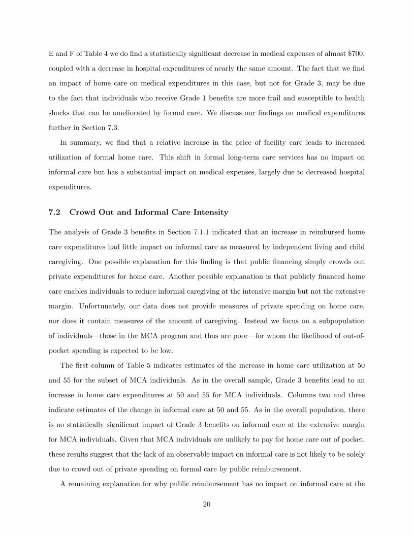
The first column of Table 5 indicates estimates of the increase in home care utilization at 50

and 55 for the subset of MCA individuals. As in the overall sample, Grade 3 benefits lead to an

increase in home care expenditures at 50 and 55 for MCA individuals. Columns two and three

indicate estimates of the change in informal care at 50 and 55. As in the overall population, there

is no statistically significant impact of Grade 3 benefits on informal care at the extensive margin

for MCA individuals. Given that MCA individuals are unlikely to pay for home care out of pocket,

these results suggest that the lack of an observable impact on informal care is not likely to be solely

due to crowd out of private spending on formal care by public reimbursement.

A remaining explanation for why public reimbursement has no impact on informal care at the

20

extensive margin is that the impact is on the intensive margin. To shed light on this possibility,

we look at the impact of Grade 3 benefits on the use of a particular home care service, short-term

respite care. Short-term respite care is short-term (i.e. a few days) facility care used to provide

temporary relief for the regular caregiver. Thus, use of this type of home care is a strong indication

for reduction in informal caregiving at the intensive margin. Indeed, as shown in Table 6, which

shows estimates for several home care services, we find Grade 3 benefits lead to a statistically

significant increase in the use of short-term respite care at 55.

Similar to Grade 3, Grade 2 benefits may lead to crowding out of facility care. To measure

the extent of crowd out, we need a measure of all facility care, regardless of whether it is financed

publicly or privately. Since we only observe publicly financed facility care in the data, we accomplish

this by using an indirect measure of all facility utilization: medical spending occurring in a long-

term care facility (i.e. regardless of financing). If the probability of having medical spending

occurring in a long-term care facility is a fixed percentage of those who attend a long-term care

facility (at the threshold), then changes in the probability of having medical spending occurring in a

long-term care facility will capture changes in the probability of attending a long-term care facility.

In other words, if# w/Medical Spending in LTC Facility

# in LTC Facilityis fixed, then a percentage increase in

the denominator will be tied to a percentage increase in the numerator of the same magnitude.18

Table 7 presents estimates of the impact at 70 and 75 of the probability of using a publicly financed

long-term care facility and the probability of having medical spending occurring in a long-term care

facility. Scoring just above 70 is associated with a 25% increase (6.5 percentage points on a base

of 25.7%) in the probability of using publicly financed facility care. However, using the probability

of medical spending occurring in a long-term care facility as a proxy for all facility care shows that

the probability of using facility care, regardless of financing, increases only 18% (2.9 percentage

points on a base of 15.6%) at 70. This suggests that 27.4% (= 25.4−18.425.4 ) of publicly financed care is

used to substitute for out of pocket expenditures. The corresponding measure of crowd out at 75

is 46.7%. The fact that crowd out is higher at 75 than 70 is not surprising, given that individuals

at 75 have more need for long-term care and thus are more likely to privately finance facility care

18It is possible that those who spend out of pocket (i.e. those below the threshold) are likely to be sicker and thushave a higher probability of medical spending occurring in a facility. To the extent that this is the case, we will finda smaller change in the probability of having medical spending occurring in a facility and an over (upper bound)estimate of crowdout.

21

in the absence of LTCI. While these measures of crowd out are substantial, they also suggest that

crowd out is not complete, and therefore cannot fully explain our lack of findings for informal care.

7.3 LTC Expenditures and Reductions in Medical Expenses

In light of the previous results showing decreases in medical expenditure, a useful metric for assess-

ing the cost-effectiveness of this policy and its costs to the government is to compare the reimbursed

long-term care expenses to the changes in medical expenses. Recall that with the administrative

data we use, we are able to measure the both the universe of medical expenditures and the universe

of public long-term care expenditures. The first set of columns of Table 8 display the estimated

impacts of all thresholds on reimbursed long-term care expenditures. For convenience, the second

set of columns redisplay the impacts on medical expenditures. The third set of columns indicate

the medical expenditures saved per additional dollar of long-term care expenditure reimbursed.

A preliminary score above 50 and 55 leads to a $208 and $931 increase in total reimbursed long-

term care expenditures, respectively. As seen earlier, however, this results in little, if any, savings

in medical expenditures. Focusing on Grade 2, we see that additional benefits for facility care lead

to an additional $500 in expenditures as individuals substitute more expensive facility care in place

of home care. However, corresponding to this increase in expenditure we find a decrease in medical

expenditures of more than $300, for a medical expenditure savings of $0.6 per dollar of long-term

care reimbursed. The fact that there is no apparent savings at 70 may be due to heterogeneous

impacts of the policy or possible bias at 75. Focusing on Grade 1 at 95 (recall that there is little

effective change in eligibility at 90), we see that additional benefits for Grade 1 lead to only small

changes in expenditures as individuals tend to use more home care and less facility care. However,

this substitution leads to large impacts on medical expenditures—nearly a $700 reduction. Clearly,

the amount of long-term care reimbursed is not a complete measure of the costs of the program as

it does not include the administrative expenses, for example. Moreover, medical expenses are not a

complete measure of the potential cost savings of the program as impacts on labor outcomes could

have impacts on government revenue.19 However, the large impact we measure here highlights the

importance of considering the potential program savings from reduced medical expenditures.

19Our limited findings on informal care at the extensive margin suggest that these labor market impacts may besmall.

22

8 Robustness

8.1 Balance of Covariates

As discussed in Section 3.1, an important assumption for our identification strategy is that indi-

viduals on each side of the thresholds are comparable. A test of this assumption is to check the

balance of observable characteristics across the thresholds. Table 9 contains estimates of the dis-

continuities around the thresholds for predetermined variables that are likely to be correlated with

our dependent variables of interest. With the exception of the 75 threshold, most of the variables

appear to be continuous around the thresholds at our preferred bandwidth.

Because we are testing numerous variables and thresholds, some discontinuities will be statis-

tically significant by random chance. As a result, we conduct two tests which account for this,

with results presented in the last two sets of columns of Table 9. First, we look at a summary

measure—the predicted medical expenditures from a regression of medical expenditures on the

other predetermined variables. Again, with the exception of the 75 threshold, there appear to be

no discontinuities in predicted medical expenditures at our preferred bandwidth. Second, we test

whether the discontinuities are jointly significant by seemingly unrelated regression, as described

in Lee and Lemieux (2010). Consistent with the first exercise, the only threshold for which the

discontinuities are jointly significant at the preferred bandwidth is 75. This leads us to believe that

our results are not impacted by unobserved confounders at the other thresholds. Nonetheless, we

controlled for the few instances of significance occurring in our variables of interest by estimating

differences in our dependent variables in our regressions.

8.2 Differential Mortality

Another relevant outcome is whether these benefits had any impact on mortality. This measure

is important in and of itself, and is useful because it is objective and well-defined. Moreover, it is

important to address the concern that differential mortality around the thresholds could account for

our findings. For example, if individuals just below the threshold were more likely to die as a result

of not receiving treatment, relatively healthy individuals would remain in the sample, minimizing

any estimated impacts. We assess this by looking at mortality by 2010 around the thresholds.

Table 10 displays estimates of Equation 1 with mortality by 2010 as the outcome. We find no

23

statistically significant differences in mortality at all thresholds. Thus, the increase in long-term

care utilization at the thresholds has no impact on mortality in the short-run.

8.3 Other Specifications

A consequential decision in estimating Equation 1 is the choice of bandwidth. Although we have

shown that our results are qualitatively consistent at both our preferred bandwidth and the IK

bandwidth, it is useful to know how sensitive our findings are to bandwidth choice. To do so,

we reestimate Equation 1 for our main outcomes of interest at several bandwidths—from 1 to

5, in increments of 0.5. Figures B.3 to B.8 plot the estimated coefficients with 95% confidence

bands against the bandwidth. There are two things worth highlighting. First, coefficients are less

precisely estimated and more variable at very small bandwidths. Second, the coefficient estimate at

our preferred bandwidth falls within the 95% confidence bands of the estimates at other bandwidths

in general, indicating that our findings are not too sensitive to bandwidth selection.

On the specification of f(S), our approach in this paper follows Hahn, Todd, and van der

Klaauw (2001) by using local linear regressions to estimate the discontinuity at the threshold. As

shown in the previous section, our findings are consistent even at very small bandwidths. Moreover,

visual inspection suggests the relationship between eligibility (as well as our outcomes of interest)

and the preliminary score is fairly linear even at relatively large distances from the thresholds.

Nonetheless, in Figures B.9 to B.14 we explore how sensitive our findings are to higher order

specifications of f(S) at our preferred bandwidth. For the most part, the coefficient estimate based

on a linear specification of f(S) falls within the 95% confidence bands of estimates for higher order

specifications. However, the variance of the higher order specifications grows quite large, which

lends support for the use of linear splines.

8.4 Differences-in-Differences Estimation

Our research design takes advantage of a setting with a continuous measure of long-term care

needs (i.e. the preliminary score) and thresholds that lead to “as good as random” variation in

the probabilities of benefits. One limitation of this design, however, is the reduced precision from

relying primarily on observations around the threshold. In this section, we estimate a differences-

in-differences model that relies on stronger assumptions, but has potentially improved precision.

24

Specifically, we compare three groups of individuals: individuals who are treated based solely on

the preliminary score (for Grade 3, we consider individuals with preliminary scores in [55,60)),

individuals who are treated based on committee guidelines (for Grade 3, these are individuals with

preliminary scores in [50,55)), and individuals who are not treated (for Grade 3, these are individuals

with preliminary scores in [45,50)). For τ ∈ {55, 75, 95}, we define commitτ ≡ 1I{τ − 5 ≤ S < τ}

and treatτ ≡ 1I{τ ≤ S < τ + 5}, where S is the 2009 preliminary score. With the untreated

individuals (i.e. {S : τ − 10 ≤ S < τ − 5}) as the reference group, we estimate the following

differences-in-differences model for an individual i at time t:

outcomeit =

1∑t=0

(βCt commitτ · t+ βTt treatτ · t) + φ · t+ εit, (2)

where t is 0 in the baseline year and 1 in the following year.20 The key assumption underlying this

estimation method is that there are no unobserved factors that affect the three groups differentially

over time.

Table 11 presents estimates of βC1 and βT1 from Equation 2. Grade 3 expenditures lead to

a statistically significant decrease in child caregiving, but have no statistically significant impact

on independent living. There is no statistically significant impact on medical expenditures or

hospital expenses. Additional long-term care expenditures resulting from Grade 2 benefits are also

associated with a statistically significant decrease in child caregiving, but not independent living.

The use of Grade 2 benefits leads to a decrease in other medical expenses, accounted for largely

by hospital expenses. These results translate into a medical dollars saved per additional dollar of

reimbursed long-term care expenditure of 0.3. The use of Grade 1 benefits leads to a decrease in

other medical expenses, largely accounted for by hospital expenses. In this case, the medical dollars

saved per additional dollar of reimbursed long-term care expenditure is more than one, suggesting

strong program savings.

The findings from this analysis are fairly consistent with our findings from the regression discon-

tinuity analysis. Even though the differences-in-differences analysis suggests statistically significant

impacts on child caregiving while RD estimates do not, this could be due to lack of statistical pre-

20Recall that the baseline year is 2008 for the medical expenditure related (NHI) variables and 2009 for all other(NLTCI) variables.

25

cision. Moreover, estimates of medical expenditures saved per dollar of reimbursed long-term care

are similar across both estimation strategies.

Lastly, this estimation strategy allows us to compare the committee affected group to the auto-

matically treated group. This is particularly relevant given that assigning treatment based solely

on the preliminary score may not be optimal and that leaving room for discretionary assignment

of treatment may improve efficiency. In this analysis, there do not appear to be any striking dif-

ferences in performance between the two groups among Grades 3 and 2 individuals. However, it

appears that the committee affected group has a more substantial impact among Grade 1 affected

individuals. While this suggests the possibility that a more discretionary decision-making proce-

dure for determining treatment may be more effective than a hard rules-based criteria, we caution

that this measure (vs. quality of life, for example) may not be the primary objective to optimize

from the standpoint of the committee.

9 Discussion

In this paper, we find that publicly financed long-term care leads to small, if any, impacts on

informal care at the extensive margin. We determine that this is not solely due to crowdout, but

partly explained by the fact that informal care is reduced at the intensive margin. That we find

limited impacts on informal care stands in contrast to some of the previous literature, but is not

surprising given that family ties are relatively stronger in South Korea. That is, due to family

obligations, Koreans may find it more difficult to give up completely the responsibility of taking

care of their elderly parents. That we still find reductions in the intensive margin indicate that

our results constitute a lower bound for the effect in the U.S., and may be directly indicative of

countries with relatively stronger family ties, such as many developing countries, and immigrant

populations from those countries.

Interestingly, we find that among less able individuals, transitioning from home to facility care

results in decreased medical expenditures. This may come as a surprise at first, given that the

purpose of long-term care is not so much to restore or maintain health as it is to increase the

general welfare of the individual by facilitating activities of daily living. Indeed, we find no impacts

on health as captured by mortality. However, a plausible explanation is that the increased attention

26

one receives in a facility may prevent costly accidents like falling and breaking one’s hip. Another

possibility is that patients are able to transition sooner out of more expensive hospital care and

into less expensive facility care. Surprisingly, among the least able, the opposite transition leads to

substantially lower medical expenses. This may be mediated by the fact that the presence of medical

professionals in a facility may lead to additional or more costly care than if one were being cared for

at the home, and that, among this population of individuals, this effect predominates the previously

mentioned effects. In fact, that transitioning people from institutions to the community may be

beneficial is consistent with the objectives of programs such as Money Follows the Person in the

U.S. This supports the more general point that our findings on medical expenses are not culturally

or context specific, and that understanding the relationship between long-term care expenses and

medical expenses may be a fruitful avenue to contain health care costs.

10 Conclusion

Results from this paper provide insight into the welfare impacts of government reimbursement of

long-term care on care recipients, caregivers, and taxpayers, as well as suggestions for the design

of optimal long-term care policy. Our main finding is that the benefits of home and facility care

are heterogeneous across physical function level and therefore setting policy accordingly has the

potential to dramatically reduce medical expenses. We also find that formal long-term care is not

a strong substitute for informal long-term care at the extensive margin.

Among more able individuals, we find that government subsidies for formal home care lead to

an overall increase in its utilization, even accounting for crowd out, with no impact on informal

caregiving at the extensive margin, medical expenses, or mortality. While we find evidence for a

reduction in informal caregiving at the intensive margin, this suggests that if the policy objective

is to increase the labor supply of individuals caring for this population, subsidies for home care

may have little impact. Moreover, the converse of our findings on medical expenses and mortality

suggest that home care reimbursement may be reduced without significant detriment to the health

of the care recipient.

Among less able individuals, additional reimbursement of institutional care leads to an overall

increase in its utilization, despite up to 47% being used to substitute for out-of-pocket expenses, and

27

corresponding reductions in informal caregiving and medical expenses. From a policy perspective,

the latter finding suggests that while substitution of institutional care for less expensive home

care may lead to increased costs, this may be partially offset by reductions in medical expenses.

Moreover, our finding on informal caregiving suggests that this policy may lead to increased labor

supply of individuals caring for this population. In this case, optimal policy depends on the objective

function of the policymaker in balancing the tradeoff between increased taxpayer costs, reduced

informal caregiving, and improved quality of life for the care recipient.

Among the least able, we find that an increase in the price of institutional care combined with an

increase in the benefit maximum for home care leads to substitution of home care for institutional

care. While we find no impact on informal caregiving, we find substantial decreases in medical

spending. From a policy perspective, this suggests that increased incentives for the use of home

care may lead to an improvement in the welfare of care recipients while limiting or even reducing

costs to taxpayers.

28

Table 1: Overview of Grades of Benefits

29

Table 2: Summary Statistics by Grade

Notes: Sample consists of individuals who were assessed for long-term care insurance in 2008 and 2009.

Grade categorization is based on the 2009 adjusted score. All measures are at baseline, except for long-term

care facility days and home care expenditures. See text for definitions of variables.

30

Table 3: Effect of Thresholds on Changes in Eligibility

(a)

(b)

(c)

Notes: The first two columns of each panel report estimates of β from local linear regression of Equation (1).

Each cell represents a different regression. The running variable is the 2009 preliminary score. Controls

include age, gender, region type, insurance type, and insurance contribution. Rectangular kernel. The third

column of each panel reports the optimal bandwidth determined by the IK procedure. Robust standard

errors in parentheses. ** p < 0.01, * p < 0.05, + p < 0.1.

31

Table 4: Main Results on LTC Utilization, Informal Care, and Medical Expenditures

Notes: The first two columns of each panel in this table report estimates of β from local linear regression of Equation (1). Each cell represents a

different regression. The running variable is the 2009 preliminary score. Controls include age, gender, region type, insurance type, and insurance

contribution. Rectangular kernel. The third column of each panel reports the optimal bandwidth determined by the IK procedure. Robust standard

errors in parentheses. ** p < 0.01, * p < 0.05, + p < 0.1.

32

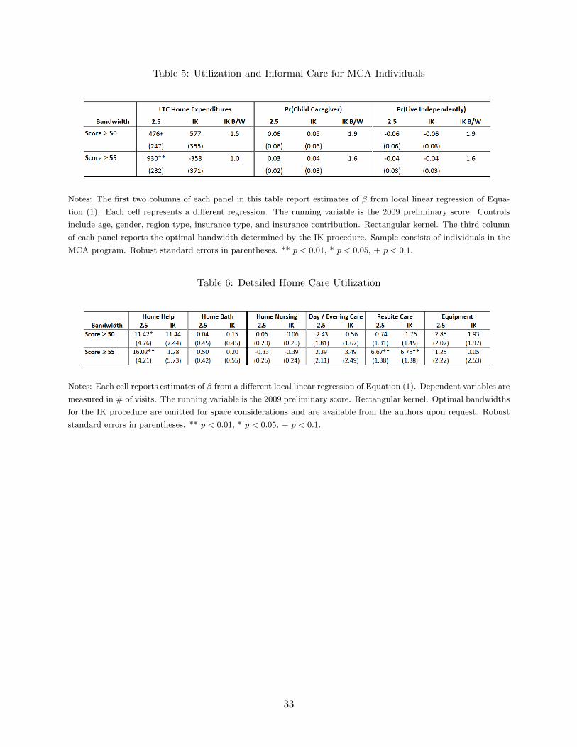
Table 5: Utilization and Informal Care for MCA Individuals

Notes: The first two columns of each panel in this table report estimates of β from local linear regression of Equa-

tion (1). Each cell represents a different regression. The running variable is the 2009 preliminary score. Controls

include age, gender, region type, insurance type, and insurance contribution. Rectangular kernel. The third column

of each panel reports the optimal bandwidth determined by the IK procedure. Sample consists of individuals in the

MCA program. Robust standard errors in parentheses. ** p < 0.01, * p < 0.05, + p < 0.1.

Table 6: Detailed Home Care Utilization

Notes: Each cell reports estimates of β from a different local linear regression of Equation (1). Dependent variables are

measured in # of visits. The running variable is the 2009 preliminary score. Rectangular kernel. Optimal bandwidths

for the IK procedure are omitted for space considerations and are available from the authors upon request. Robust

standard errors in parentheses. ** p < 0.01, * p < 0.05, + p < 0.1.

33

Table 7: Crowd Out of Facility Care

Notes: Columns 1 and 2 report coefficient estimates from Equation (1). Dependent variables are indicators for public

reimbursement of facility care and medical spending in a LTC facility. The running variable is the 2009 preliminary

score. Rectangular kernel. “Change at ‘X’ ” is the estimate of β. “Base at ‘X’ ” is the predicted value of the

dependent variable at ‘X’ minus the “Change at ‘X’ ”. ** p < 0.01, * p < 0.05, + p < 0.1.

34

Table 8: LTC Expenses vs. Medical Care Savings

Notes: The first two columns of the first two panels in this table report estimates of β from local linear regression of

Equation (1). Each cell represents a different regression. The running variable is the 2009 preliminary score. Controls

include age, gender, region type, insurance type, and insurance contribution. Rectangular kernel. The third columns

report the optimal bandwidth determined by the IK procedure. Robust standard errors in parentheses. ** p < 0.01,

* p < 0.05, + p < 0.1. The third panel equals the coefficient in the second panel divided by the coefficient in the first

panel.

35

Table 9: Covariate Balance

Notes: Columns 1-6 and 8 report estimates of β from local linear regression of Equation (1). Each cell represents a different regression. Dependent variables

are 2008 measures. The running variable is the 2009 preliminary score. Rectangular kernel. Optimal bandwidths for the IK procedure are omitted for space

considerations and are available from the authors upon request. Robust standard errors in parentheses. ** p < 0.01, * p < 0.05, + p < 0.1. Column 7 reports the

p-value from a joint test of the coefficients in each row from a SUR where the bandwidth is 2.5.

36

Table 10: Effect of Eligibility on Mortality

Notes: The first two columns of this table report estimates of β from local linear regression of Equation (1). Each

cell represents a different regression. The dependent variable is mortality by 2010. The running variable is the 2009

preliminary score. Controls include age, gender, region type, insurance type, and insurance contribution. Rectangular

kernel. The third column of each panel reports the optimal bandwidth determined by the IK procedure. Robust

standard errors in parentheses. ** p < 0.01, * p < 0.05, + p < 0.1.

37

Table 11: Differences-in-Differences Estimates

38

Figure 1: Adjusted Scores vs. Preliminary Scores, 2009

Notes: This figure plots the 2009 adjusted score against the 2009 preliminary score, for individuals whose

preliminary scores fall between 45 and 105. Circle sizes correspond to the number of individuals with the

associated adjusted/preliminary score combination.

2009 adjusted score = 2009 preliminary score + committee points, where committee points ∈ [−5, 5].

39

Figure 2: Probability of Eligibility vs. 2009 Preliminary Score

(a) Grade 3 Eligibility

(b) Grade 2 Eligibility

(c) Grade 1 Eligibility

Notes: The running variable is the 2009 preliminary score. The open circles plot the mean of the dependent

variable within 0.2 point bins. The solid lines are fitted values from local linear regression of the dependent

variable using a rectangular kernel with a bandwidth of 2.5 points. The shaded regions are 95 percent

confidence intervals.

40

Figure 3: Histograms of Scores

(a) Around Grade 3 Thresholds

(b) Around Grade 2 Thresholds

(c) Around Grade 1 Thresholds

Notes: 2009 preliminary score in 0.1 point bins.

41

Figure 4: Impact of ↑ sH on A, C, and H

Figure 5: Impact of ↑ sF on A, H, and F

42

Figure 6: Impact of ↑ mH on A, C, and H

(a) H1 < mH (b) H1 = mH

43

Figure 7: Reimbursed Formal Care Utilization vs. Preliminary Score Around Grade 3

(a) Home Care Expenditures

(b) Institutional Days

Notes: The running variable is the 2009 preliminary score. The open circles plot the mean of the dependent

variable within 0.2 point bins. The solid lines are fitted values from local linear regression of the dependent

variable using a rectangular kernel with a bandwidth of 2.5 points. The shaded regions are 95 percent

confidence intervals.

44

Figure 8: Change in Informal Care vs. Preliminary Score Around Grade 3

(a) ∆ Pr(Live Independently)

(b) ∆ Pr(Child Caregiver)

Notes: The running variable is the 2009 preliminary score. The open circles plot the mean of the dependent

variable within 0.2 point bins. The solid lines are fitted values from local linear regression of the dependent

variable using a rectangular kernel with a bandwidth of 2.5 points. The shaded regions are 95 percent

confidence intervals.

45

Figure 9: Change in Medical Utilization vs. Preliminary Score Around Grade 3

(a) ∆ Medical Expenses

(b) ∆ Hospital Expenses

Notes: The running variable is the 2009 preliminary score. The open circles plot the mean of the dependent

variable within 0.2 point bins. The solid lines are fitted values from local linear regression of the dependent

variable using a rectangular kernel with a bandwidth of 2.5 points. The shaded regions are 95 percent

confidence intervals.

46

Figure 10: Reimbursed Formal Care Utilization vs. Preliminary Score Around Grade 2

(a) Home Care Expenditures

(b) Institutional Days

Notes: The running variable is the 2009 preliminary score. The open circles plot the mean of the dependent

variable within 0.2 point bins. The solid lines are fitted values from local linear regression of the dependent

variable using a rectangular kernel with a bandwidth of 2.5 points. The shaded regions are 95 percent

confidence intervals.

47

Figure 11: Change in Informal Care vs. Preliminary Score Around Grade 2

(a) ∆ Pr(Live Independently)

(b) ∆ Pr(Child Caregiver)

Notes: The running variable is the 2009 preliminary score. The open circles plot the mean of the dependent

variable within 0.2 point bins. The solid lines are fitted values from local linear regression of the dependent

variable using a rectangular kernel with a bandwidth of 2.5 points. The shaded regions are 95 percent

confidence intervals.

48

Figure 12: Change in Medical Utilization vs. Preliminary Score Around Grade 2

(a) ∆ Medical Expenses

(b) ∆ Hospital Expenses

Notes: The running variable is the 2009 preliminary score. The open circles plot the mean of the dependent

variable within 0.2 point bins. The solid lines are fitted values from local linear regression of the dependent

variable using a rectangular kernel with a bandwidth of 2.5 points. The shaded regions are 95 percent

confidence intervals.

49

Figure 13: Reimbursed Formal Care Utilization vs. Preliminary Score Around Grade 1

(a) Home Care Expenditures

(b) Institutional Days

Notes: The running variable is the 2009 preliminary score. The open circles plot the mean of the dependent

variable within 0.2 point bins. The solid lines are fitted values from local linear regression of the dependent

variable using a rectangular kernel with a bandwidth of 2.5 points. The shaded regions are 95 percent

confidence intervals.

50

Figure 14: Change in Informal Care vs. Preliminary Score Around Grade 1

(a) ∆ Pr(Live Independently)

(b) ∆ Pr(Child Caregiver)

Notes: The running variable is the 2009 preliminary score. The open circles plot the mean of the dependent

variable within 0.2 point bins. The solid lines are fitted values from local linear regression of the dependent

variable using a rectangular kernel with a bandwidth of 2.5 points. The shaded regions are 95 percent

confidence intervals.

51

Figure 15: Change in Medical Utilization vs. Preliminary Score Around Grade 1

(a) ∆ Medical Expenses

(b) ∆ Hospital Expenses

Notes: The running variable is the 2009 preliminary score. The open circles plot the mean of the dependent

variable within 0.2 point bins. The solid lines are fitted values from local linear regression of the dependent

variable using a rectangular kernel with a bandwidth of 2.5 points. The shaded regions are 95 percent

confidence intervals.

52

References

CBO. 2007. The Long-Term Outlook for Health Care Spending. Congressional Budget Office.

Charles, KK and P Sevak. 2005. “Can Family Caregiving Substitute for Nursing Home Care?”

Journal of Health Economics 24 (6):1174–1190.

Christianson, JB. 1988. “The Evaluation of the National Long-Term Care Demonstration .6. The

Effect of Channeling on Informal Caregiving.” Health Services Research 23 (1):99–117.

Colombo, F., A. Llena-Nozal, J. Mercier, and F. Tjadens. 2011. Help Wanted? Providing and

Paying for Long-Term Care. OECD Health Policy Studies. OECD Publishing.

Engelhardt, Gary V and Nadia Greenhalgh-Stanley. 2010. “Home Health Care and the Housing

and Living Arrangements of the Elderly.” Journal of Urban Economics 67 (2):226–238.

GAO. 2005. Long-Term Care Financing: Growing Demand and Cost of Services are Straining

Federal and State Budgets. U.S. Government Accountability Office.

Golberstein, E, DC Grabowski, KM Langa, and ME Chernew. 2009. “Effect of Medicare Home

Health Care Payment on Informal Care.” Inquiry 46 (1):58–71.

Imbens, Guido and Karthik Kalyanaraman. 2009. “Optimal Bandwidth Choice for the Regression

Discontinuity Estimator.” Working Paper 14726, National Bureau of Economic Research.

Lee, David S. 2008. “Randomized Experiments from Non-Random Selection in US House Elections.”

Journal of Econometrics 142 (2):675–697.

Lee, David S and Thomas Lemieux. 2010. “Regression Discontinuity Designs in Economics.” Jour-

nal of Econometric Literature 48 (2):281–355.

Lo Sasso, AT and RW Johnson. 2002. “Does Informal Care from Adult Children Reduce Nursing

Home Admissions for the Elderly?” Inquiry 39 (3):279–297.

McKnight, R. 2006. “Home Care Reimbursement, Long-Term Care Utilization, and Health Out-

comes.” Journal of Public Economics 90 (1-2):293–323.

53

Orsini, Chiara. 2010. “Changing the Way the Elderly Live: Evidence from the Home Health care

Market in the United States.” Journal of Public Economics 94 (1-2):142–152.

Pezzin, LE, P Kemper, and J Reschovsky. 1996. “Does Publicly Provided Home Care Substitute

for Family Care? Experimental Evidence with Endogenous Living Arrangements.” Journal of

Human Resources 31 (3):650–676.

Stabile, Mark, Audrey Laporte, and Peter C. Coyte. 2006. “Household Responses to Public Home

Care Programs.” Journal of Health Economics 25 (4):674–701.

Urquiola, Miguel and Eric Verhoogen. 2009. “Class-Size Caps, Sorting, and the Regression-

Discontinuity Design.” American Economic Review 99 (1):179–215.

Van Houtven, CH and EC Norton. 2004. “Informal Care and Health Care Use of Older Adults.”

Journal of Health Economics 23 (6):1159–1180.

Ward, Derek, Amy Drahota, Diane Gal, Martin Severs, and Taraneh P. Dean. 2008. “Care Home

Versus Hospital and Own Home Environments for Rehabilitation of Older People.” Cochrane

Database of Systematic Reviews (4).

Wooldridge, J and J Schore. 1988. “The Evaluation of the National Long-Term Care Demonstra-

tion .7. The Effect of Channeling on the Use of Nursing Homes, Hospitals, and Other Medical

Services.” Health Services Research 23 (1):119–127.

A Calculation of the Preliminary Score

The preliminary score is calculated from the responses to 52 questions in the eligibility evaluation.

A list of these items and possible responses are listed in Table A.1.

The procedure for determining the preliminary score is as follows:

1. Convert responses to point values, according to Table A.1.

2. Sum the points in each category.

3. Based on the category scores and the responses to the 52 items, determine sub-scores for eight

service categories: individual hygiene, excretion support, eating, moving, behavior, indirect

54

support, nursing care, and rehabilitation. See Figure A.1 for an illustration of how the eating

sub-score is determined.

4. Sum the service sub-scores to arrive at the preliminary score.

We now provide a partial example for calculating the preliminary score. Table A.2 contains

a sample set of answers to the eligibility assessment. The category scores for ADL and REH are

16 and 13, respectively. Now follow the eating tree. The first fork depends on the response to

“eating” in the ADL category. The response of independent (1) sends us along the left branch.

The response to ”brushing teeth” is independent (1), which takes us down the first branch. Since

the ADL score is 16, we end up along the right branch for a score of 9.4. We repeat this procedure

for the remaining service sub-scores:

• Individual hygiene 5.3

• Excretion support 2.6

• Eating 9.4

• Moving 3.6

• Behavior 0.8

• Indirect 21.7

• Nursing Care 9.7

• Rehabilitation 2.7

These sum to the final score of 55.8.

55

Table A.1: Assessment Questions

56

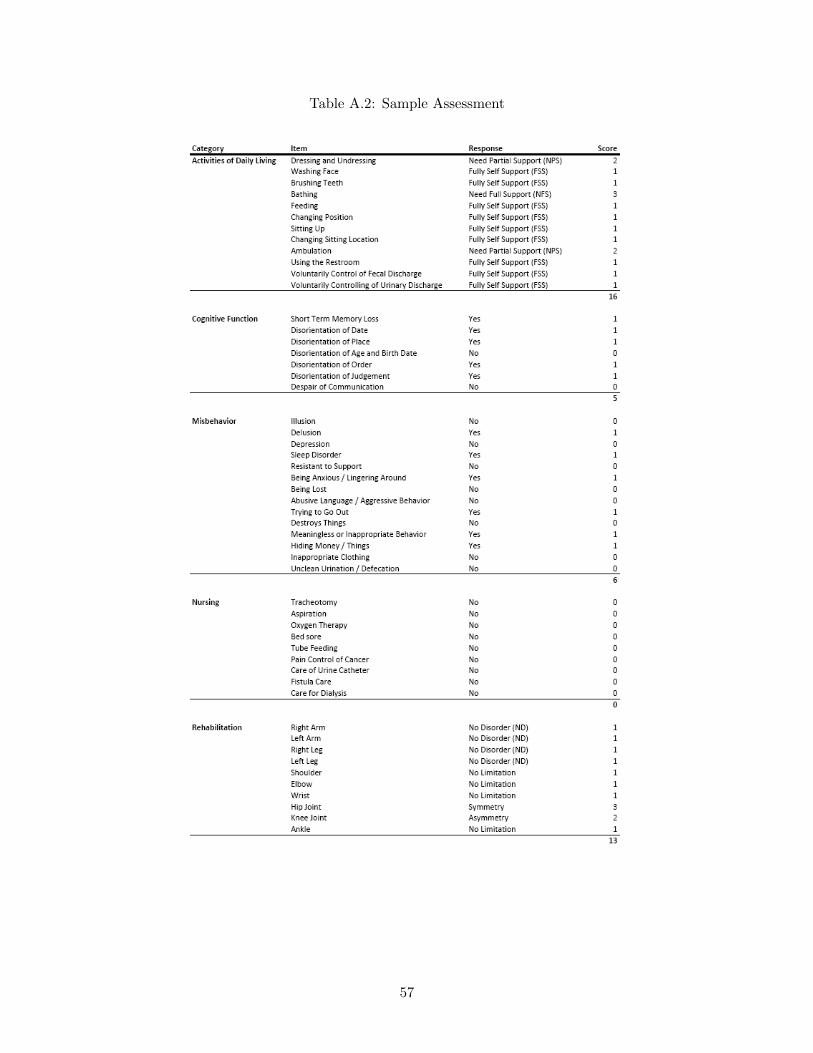
Table A.2: Sample Assessment

57

Figure A.1: Eating Tree

58

B Supplemental Tables and Figures

59

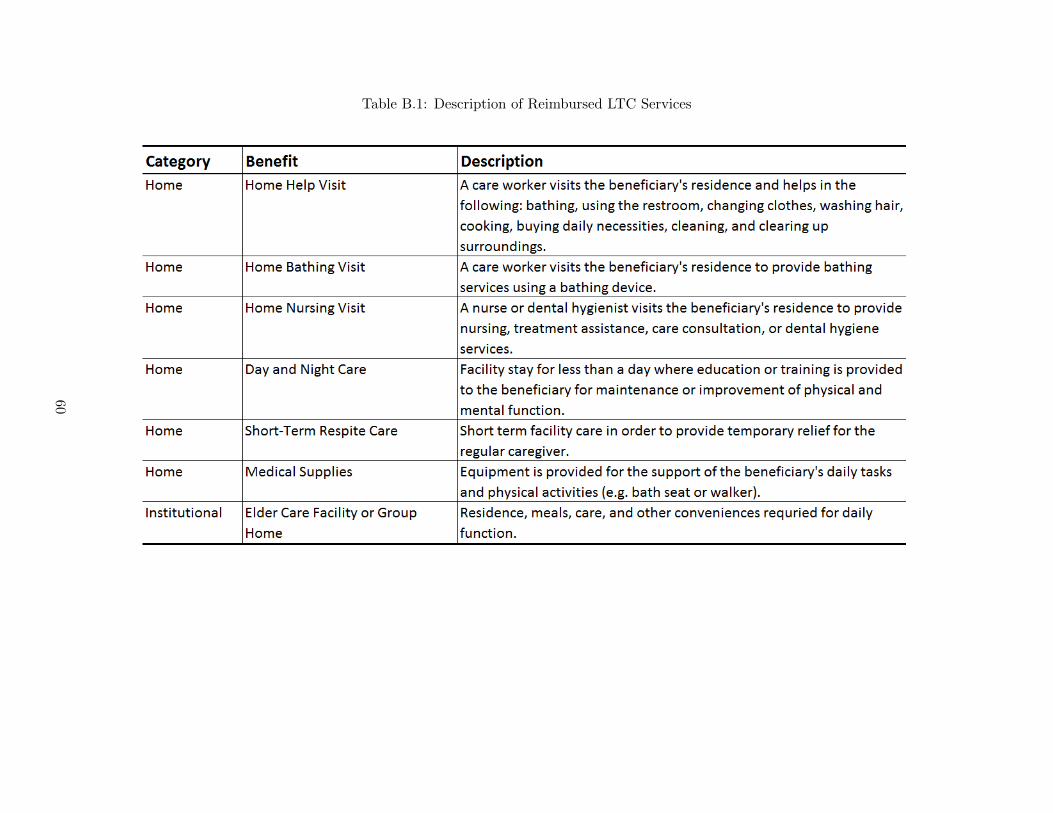
Table B.1: Description of Reimbursed LTC Services

60

Figure B.1: Density of Scores, 2009 vs. April 2008

(a) (b)

Notes: Preliminary scores in 1 point bins. “All 2009” consists of the preliminary scores from assessments in 2009. “April 2008” consists of the

preliminary scores from assessments in April 2008.

61

Figure B.2: Score Sensitivity Example

Notes: Sample of individuals whose preliminary scores fall between 45 and 105, with the response “Fully

Independent” to the item “Changing Position”. The original preliminary score is on the x-axis. The new

preliminary score after changing the response from “Fully Independent” to “Needs Partial Support” is on

the y-axis. Also graphed in red is the 45 degree line.

62

Figure B.3: Sensitivity to Bandwidth at 50

(a) LTC Expenditures (b) Medical Expenditures

(c) Child Caregiving (d) Independent Living

Notes: Each figure displays estimates of β from local linear regression of Equation (1) at different bandwidths

in increments of 0.5, from 1 to 5. Each figure corresponds to a different outcome.

63

Figure B.4: Sensitivity to Bandwidth at 55

(a) LTC Expenditures (b) Medical Expenditures

(c) Child Caregiving (d) Independent Living

Notes: Each figure displays estimates of β from local linear regression of Equation (1) at different bandwidths

in increments of 0.5, from 1 to 5. Each figure corresponds to a different outcome.

64

Figure B.5: Sensitivity to Bandwidth at 70

(a) LTC Expenditures (b) Medical Expenditures

(c) Child Caregiving (d) Independent Living

Notes: Each figure displays estimates of β from local linear regression of Equation (1) at different bandwidths

in increments of 0.5, from 1 to 5. Each figure corresponds to a different outcome.

65

Figure B.6: Sensitivity to Bandwidth at 75

(a) LTC Expenditures (b) Medical Expenditures

(c) Child Caregiving (d) Independent Living

Notes: Each figure displays estimates of β from local linear regression of Equation (1) at different bandwidths

in increments of 0.5, from 1 to 5. Each figure corresponds to a different outcome.

66

Figure B.7: Sensitivity to Bandwidth at 90

(a) LTC Expenditures (b) Medical Expenditures

(c) Child Caregiving (d) Independent Living

Notes: Each figure displays estimates of β from local linear regression of Equation (1) at different bandwidths

in increments of 0.5, from 1 to 5. Each figure corresponds to a different outcome.

67

Figure B.8: Sensitivity to Bandwidth at 95

(a) LTC Expenditures (b) Medical Expenditures

(c) Child Caregiving (d) Independent Living

Notes: Each figure displays estimates of β from local linear regression of Equation (1) at different bandwidths

in increments of 0.5, from 1 to 5. Each figure corresponds to a different outcome.

68

Figure B.9: Sensitivity to Polynomial Degree at 50

(a) Medical Expenditures

(b) Child Caregiving

Notes: Each figure displays estimates of β from local linear regression of Equation (1) at different polynomial

degrees, from 1 to 4. Bandwidth is 2.5. Each figure corresponds to a different outcome.

69

Figure B.10: Sensitivity to Polynomial Degree at 55

(a) Medical Expenditures

(b) Child Caregiving

Notes: Each figure displays estimates of β from local linear regression of Equation (1) at different polynomial

degrees, from 1 to 4. Bandwidth is 2.5. Each figure corresponds to a different outcome.

70

Figure B.11: Sensitivity to Polynomial Degree at 70

(a) Medical Expenditures

(b) Child Caregiving

Notes: Each figure displays estimates of β from local linear regression of Equation (1) at different polynomial

degrees, from 1 to 4. Bandwidth is 2.5. Each figure corresponds to a different outcome.

71

Figure B.12: Sensitivity to Polynomial Degree at 75

(a) Medical Expenditures

(b) Child Caregiving

Notes: Each figure displays estimates of β from local linear regression of Equation (1) at different polynomial

degrees, from 1 to 4. Bandwidth is 2.5. Each figure corresponds to a different outcome.

72

Figure B.13: Sensitivity to Polynomial Degree at 90

(a) Medical Expenditures

(b) Child Caregiving

Notes: Each figure displays estimates of β from local linear regression of Equation (1) at different polynomial

degrees, from 1 to 4. Bandwidth is 2.5. Each figure corresponds to a different outcome.

73

Figure B.14: Sensitivity to Polynomial Degree at 95

(a) Medical Expenditures

(b) Child Caregiving

Notes: Each figure displays estimates of β from local linear regression of Equation (1) at different polynomial

degrees, from 1 to 4. Bandwidth is 2.5. Each figure corresponds to a different outcome.

74