Embed Size (px)
Citation preview

Munich Personal RePEc Archive
Forex Trading and the WMR Fix
Evans, Martin
Georgetown University
25 September 2017
Online at https://mpra.ub.uni-muenchen.de/81583/
MPRA Paper No. 81583, posted 27 Sep 2017 05:13 UTC

Forex Trading and the WMR Fix
(forthcoming, Journal of Banking and Finance)
Martin D.D. Evans∗
September 25, 2017
Abstract
I examine the behavior of forex prices around the setting of the 4:00 pm WMR Fix. Numerous
banks have been fined by regulators for their trading activities around the Fix, but the overall impact
of their actions is not known. I first examine trading patterns around the Fix in a microstructure model
of competitive trading. I then compare the model with the empirical behavior of forex prices across
21 currencies over a decade. Contrary to the predictions of the model, forex price changes display
extraordinary volatility and negative serial correlation around the Fix.
Keywords: Forex Trading, Order Flows, Forex Price Fixes, Microstructure Trading
Models. JEL Codes: F3; F4; G1.
∗Georgetown University, Department of Economics, Washington DC 20057. Tel: (202) 687-1570 email:[email protected]. This paper has benefited from the views of conference participants at NYU in May2015, and at Cambridge (U.K.) in June 2016. I am also grateful to the Editor and two anonymous referees fortheir comments. Any remaining errors are my own. This research uses non-proprietary data and was undertakenindependently and without compensation. Since work on this paper began, I have provided expert advice to a lawfirm involved in an ongoing US court case related to the WRM Fix. To the best of my knowledge, this is the onlycase related to the WRM Fix that is currently before the courts; there are no related active court proceedings in theUK.
1

Introduction
Since 2013, law enforcement and regulatory authorities around the world have been investigating the
forex trading activities of the world’s largest banks, particularly around the time that benchmark
forex prices are determined. To date, these investigations have generated penalties and fines on the
banks totaling more than $5.6 billion and have led to the dismissal or suspension of numerous bank
employees involved in forex trading.1 The most widely used benchmarks are provided by the WM
Company and Reuters, that were based on forex transactions during a one minute window around
4:00 pm (London time). These benchmarks are colloquially known as the “London 4 pm Fix”, “the
WMR Fix” or just the “Fix”. They provide standardize forex prices that are used to value global
equity and bond portfolios, to hedge currency exposure, to write and execute derivatives contracts,
and administer custodial agreements.
This paper provides a detailed analysis of forex prices and trading around the 4:00 pm WRM
Fix (hereafter, the “Fix”). I first explain why some market participants have strong incentives
to execute forex trades at the Fix benchmark via the submission of orders to dealer banks well
before 4:00 pm.2 These so-called Fix orders were the focus of regulators’ investigations and play a
prominent role in my analysis. Next, I examine the behavior of prices and the trading patterns in
a microstructure model of competitive forex trading. The model incorporates the key institutional
features of the Fix and makes strong predictions concerning prices and trading patterns. I then
use these predictions as benchmarks in the empirical analysis that covers a decade of trading data
on 21 currency pairs. Here I examine how the behavior of forex prices around the Fix differs from
the predictions of the microstructure model.
My main findings are summarized as follows:
1. In the model’s equilibrium, Fix orders produce volatility in post-Fix price changes because
they drive trades between dealers when the Fix orders are filled. By contrast, Fix orders do
not drive dealers’ trades before the Fix. As a consequence in this model, they have no effect
on pre-Fix price changes, and do not contribute to any correlation between pre- and post-Fix
price changes.
1Details of these investigations are provided in an on-line appendix.2Hereafter, all times are local London times unless otherwise indicated.
2

2. The observed behavior of forex prices around the Fix is highly atypical and inconsistent with
the predictions of the microstructure model outlined above:
(a) The volatility in spot rates observed immediately before the Fix is highly unusual – rates
regularly jump by an amount that is very rarely seen under normal trading conditions.
The incidence of these atypically large pre-Fix rate changes is particularly high at the
end of each month. They appear to be pervasive across all currency pairs and throughout
the decade covered by the sample.
(b) The empirical correlation between pre- and post-Fix price changes is significantly neg-
ative for many currencies – particularly on the last trading day of each month. They
appear large enough to support economically attractive trading strategies.
The theoretical results in point 1 originate from the assumption that dealer-banks attempt to share
risks efficiently when they quote forex prices. This is a key assumption in earlier multi-dealer
models of forex trading (see, e.g., Lyons, 1997; Evans and Lyons, 2002 and Evans, 2011). It also
provides the theoretical foundation for the fact dealers generally do not hold open forex positions
overnight and the half-lives of the intraday positions are measured in minutes (see, e.g., Lyons,
1995 and Bjønnes and Rime, 2005). Risk-sharing plays a central role in how dealers determine the
forex prices they quote before (and at the start of) the Fix window because they want to minimize
the risk associated with filling a large aggregate imbalance in Fix orders to purchase and sell forex.
In an efficient risk-sharing equilibrium, dealers quote prices so that there is no expected aggregate
imbalance in Fix orders.
Dealers need to fill their Fix orders once the Fix benchmark is established; a task that necessi-
tates trade between dealers. The order flow generated by this inter-dealer trade reveals the actual
imbalance in Fix orders, which dealers then embed in their post-Fix price quotes (to again share
risk efficiently). It is through this trade-based information process that the (unexpected) imbalance
in Fix orders affects the post-Fix change in prices. In contrast, inter-dealer trading before the Fix
reveals nothing about the aggregate imbalance in Fix orders because individual dealers have no
incentive to trade based on the individual orders they have received. Consequently, information
about the actual aggregate imbalance in Fix orders remains dispersed across dealers before the
Fix is determined; and, as such, it has no impact on the prices dealers quote. This implication of
3

the model counters the idea that dealers should “trade ahead of” or “front run” their fix orders
(Levine, 2014).
The empirical results listed in point 2 are equally striking. Individual instances of “large”
forex price movements before the Fix have been noted previously (see, e.g., Vaugham and Finch
2013 and Melvin and Prins, 2015). I adopt a systematic approach that quantifies the degree to
which volatility before the Fix exceeds volatility at other times. And, as a result, I show that
the atypical pre-Fix volatility has been much more widespread across time and currencies than
has been documented hitherto. It appears in all 21 currency pairs and every year covered by my
data. Moreover, pre-Fix volatility is particularly high on the last trading day of the month when
Fix orders from hedgers are known to be largest (Melvin and Prins, 2015). It appears likely that
hedgers’ orders affect pre-Fix price changes, contrary to the predictions of the competitive trading
model.
My empirical results are also at odds with the model concerning the correlation between pre- and
post-Fix price changes. Dealers’ quotes in the model embed an intraday risk premium that generates
a (small) positive serial correlation in price changes around the Fix. Furthermore, Fix orders only
contribute to the volatility of post-Fix price changes, they do produce serial correlation. In contrast,
my empirical analysis reveals a significant negative serial correlation across 18 currencies. These
correlations appear large enough to support trading strategies in many currency pairs that appeared
economically attractive at the time.
In principle, there are many reasons why the predictions of the microstructure model are so
different from my empirical findings. No model can incorporate every institutional feature of actual
forex trading, so we must acknowledge the possibility that another model of competitive trading with
more features could produce predictions that are (more) consistent with the empirical evidence.
As far as I know, such models have yet to be developed. That said, we must also acknowledge
the results of the investigations into collusion among the banks. According to the U.K. Financial
Conduct Authority and the U.S. Department of Justice, the banks’ dealers shared information on
their Fix orders in order to collusively trade before the Fix in a manner that would manipulate the
benchmark to their advantage. Importantly, the banks have admitted to colluding in this manner.
So I consider whether their actions could possibly account for my empirical findings at the end of
the paper.
4

My analysis connects with three strands of the literature. The first concerns the manipulation
of securities prices; originating with Hart (1977), Vila (1989), Allen and Gale (1992), among others.
Much of this literature’s focus is on the manipulation of equity prices, with the Vitale (2000) model
of forex manipulation a notable exception. There are several important differences between equities
and forex that limit the applicability of existing models to studying manipulation of the Fix. For
example, manipulation via corners and squeezes is impractical for major currencies, while pump-
and-dump schemes requiring the release credible but false information that moves forex prices are
implausible.3 Similarly, the literature on closing equity price manipulation (see, e.g., Cushing and
Madhavan, 2000; and Hillion and Suominen, 2004, Comerton-Forde and Putnins, 2011) applies in
settings where trading (largely) stops, whereas forex trading takes place continuously. Importantly,
I document that forex trading between 4:00 and 5:00 pm is comparable in terms of volume and
liquidity to trading in the hours before the Fix. It is therefore quite inaccurate to characterize
the Fix as a “closing forex price”. The relevance of LIBOR manipulation (Abrantes-Metz et al.,
2012 and Eisl, Jankowitsch, and Subrahmanyam, 2014) to the Fix is also limited. LIBOR is based
on banks’ reports of borrowing costs, whereas the Fix is determined by the forex prices for actual
trades.4
This paper also connects to the literature on forex microstructure. The trading model I present
extends the Portfolio Shifts (PS) model developed in Lyons (1997), Evans and Lyons (2002) and
Evans (2011) to include a round of trading where the Fix benchmark price is determined. The model
allows dealers to engage in inter-dealer trade after they have received Fix orders from hedgers and
investors but before the Fix is determined. This feature enables us to study trading patterns and
price dynamics before the Fix. As King, Osler, and Rime (2013) note in their recent survey, the PS
model “has become the intellectual workhorse of the (forex) microstructure field”, so it is natural
to extend its structure to accommodate a theoretical examination of the Fix. My theoretical
analysis is also linked to the literature on the optimal execution of large trades (Bertsimas and
3The term “currency manipulation” is sometimes used to describe the actions of governments that affect forexprices. For example, Gagnon et al. (2012) define currency manipulation as occurring “when a government buys orsells foreign currency to push the exchange rate of its currency away from its equilibrium value or to prevent theexchange rate from moving toward its equilibrium value”. The focus of this paper is on manipulation by privatesector agents for profit.
4Similar to LIBOR, Japanese banks individually announce their benchmark forex prices at 10:00 am in Japan.These benchmark prices are called the Tokyo Fix. Unlike the WMR Fix, there are no formal rules governing how thebanks choose these prices, see Ito and Yamada (2015).
5

Lo, 1998 and Almgren, 2012). As Saakvitne (2016) notes, a dealer with a large Fix order faces
a similar optimal execution problem (see, also, Yamada and Ito 2017). Whereas many models in
the optimal execution literature take the price-impact of trades as exogenous, this key feature is
determined endogenously in the equilibrium of the PS model. Empirically, my results extend earlier
microstructure findings on the intraday volatility of forex prices (see. e.g., Bollerslev and Melvin,
1994 and Ito, Lyons, and Melvin, 1998).5
The third strand of the literature explicitly focuses on the WMR Fix. Melvin and Prins (2015)
describe how currency hedging by international equity portfolio managers generates a flow of Fix
orders, and estimate a simple model for this flow at the end of each month. They then show
that intraday returns are positively related to their estimated flows before the Fix and negative
related after the Fix. My analysis builds on Melvin and Prins (2015) in two respects. First, my
microstructure model examines how the Fix orders of hedgers interact with the optimal trading
decisions of other market participants to determine the intraday dynamics of forex prices in a
competitive setting. Second, my empirical analysis covers a wider range of currency pairs over a
longer time period than has been undertaken hitherto, including the examination of intra-month
and end-of-month data. My empirical findings concerning the presence of negative serial correlation
in price changes around the WRM Fix have been confirmed by Ito and Yamada (2015).6
The remainder of the paper is structured as follows: Section 1 describes the institutional details
of the Fix and provides aggregate statistics on the importance of trading around 4:00 pm. Section
2 presents the microstructure model and examines its implications. The empirical analysis is
contained in Section 3. Section 4 provides economic perspectives on the empirical results. Section
5 concludes. Mathematical details of the model and additional statistical results are contained in
an on-line appendix.
5The patterns of high volatility and serial correlation I document are also similar to those found in equity pricesat the market’s close (Cushing and Madhavan, 2000). More generally, Hendershott and Menkveld (2014) show howserial correlation can arise in equity price changes from intermediaries shading prices to control their inventories.However, Bjønnes and Rime (2005), Osler, Mende, and Menkhoff (2011) and others find that forex dealers do notcontrol their inventories by price shading.
6My empirical results were first made public when working paper version of this article was posted on the SSRNwebsite (https://www.ssrn.com) in August 2014. Ito and Yamada (2015) found a similar but weaker serial correlationpattern in price changes around the Tokyo Fix, together with greater volatility.
6

1 Background
The WMR Fixes were established as a financial benchmark in 1993. Morgan Stanley Capital
International (MSCI) announced that after December 31st. 1993 it would use the benchmark
forex prices compiled at 4:00 pm by the WM Company and Reuters to value the foreign security
positions in its MSCI equity indices.7 Since then, the Fix benchmarks have become the de facto
standard for construction of indices comprising international securities, and have been incorporated
into numerous other tracking indices and derivatives.8 They are also routinely used to compute
the returns on portfolios that contain foreign-currency denominated securities as well as the value
of foreign securities held in custodial accounts. Fixes are now computed every half-hour for 21
currency pairs and hourly for 160 currency pairs, but the 4:00 pm Fix remains the most prominent
forex benchmark.
My empirical analysis covers forex trading from the start of 2004 until the end of 2013. This
decade includes the period investigated by law enforcement and regulatory authorities. At the
time, the WMR Fix benchmark was computed from the medians of the bid, offer and transaction
rates sampled every second from the electronic trading platforms run by Reuters and Electronic
Broking Services (EBS) over a one minute window starting 30 seconds before 4:00 pm.9 While
these platforms were the main venues for trades between dealer-banks, market participants could
also trade on a variety of other platforms. Thus, the Fix benchmark was determined by a subset
of trade rates around 4:00 pm. The methodology also took no account of trading volume.
The economic importance of the Fix arises from its use in the valuation of other securities (e.g.,
equity portfolios and derivatives) because this creates strong incentives to trade in and around the
Fix window. These incentives originate with two groups of market participants. The first comprises
those wishing to hedge currency risk. As Melvin and Prins (2015) stress, fund managers with cross-
boarder equity investments are important members of this group. Because the performance of their
investments is often tracked against the returns on the MSCI indices, many managers will want to
7Initially, the Fix benchmarks were used to compute the MSCI indices for all but the Latin American countries.After 2000, they were used for all the country indices.
8See, for example, Dow Jones Islamic Market, Global Real Estate (FTSE EPRA/NAREIT) and Global Coal(NASDAQ OMX) indices, the USD volatility warrants issued by Goldman Sacks; Wiener Borse AG fInancial futuresand CME spot, forward and swaps.
9After the disclosure that regulators were investigating forex trading, the WM Company announced a change inits methodology in October 2014. The appendix contains a complete description of the old WMR methodology.
7

reduce the tracking error of their own portfolios by choosing to hedge some of their forex exposure
to the Fix. In principle, this hedging could take place continuously through the adjustment of forex
forward positions, but in practice managers typically adjust their hedge positions at the end of each
month. This hedging activity produces orders to purchase or sell forex. And, since the managers
are concerned with tracking the MSCI indices, they want their forex orders to be filled at the Fix
to minimize the tracking error in their own portfolio’s performance. The use of Fixes in derivative
contracts produces a similar incentive to submit forex orders to be filled at the Fix from others
wishing to hedge their derivative positions. Thus, the use of Fixes in real-time valuation produces
a hedging incentive for the submission of Fix orders to dealer-banks (particularly at the end of each
month). By market convention, these orders must be submitted to dealer-banks before the 3:45
pm.
The second group of market participants affected by the Fix is the dealer-banks that accept
Fix orders. These orders differ from standard currency orders because the dealer-banks agree to
fill them at the Fix rate at least 15 minutes before that rate is determined. Thus, in effect, the
dealer-banks are offering a guarantee that the order will be filled at a particular point in time
whatever the prevailing Fix rate might be.10 By contrast, in accepting a standard forex order,
the dealer-bank undertakes to fill the order immediately at the best available prevailing rate.11 Of
course, such guarantees represent a source of risk to the dealer-bank. It is the desire to manage
this risk that creates incentives for dealer-banks to trade in and around the Fix.
Forex trading is heavily concentrated around the Fix. Panel A of Table 1 reports the ratio
of trading volume per minute at the WMR and ECB Fixes relative to the average volume per
minute between 7:00 am and 5:00 pm (excluding the Fix window) for three major currency pairs.
These statistics are computed from EBS trading data spanning three months in each of 2007, 2010
and 2013. They show that trading volume is on average far higher during the WMR Fix than at
other times, particularly at the end of the month. For comparison purposes, the table also reports
volume ratios for the 12:15 pm ECB Fix. While trading volumes for the EURUSD and GBPUSD
are above normal, they are well below the 4:00 pm WMR Fix levels. Trading volumes are even
lower for the other hourly WMR fixes. These statistics confirm that the 4:00 pm Fix is by far the
10While these are not legally binding guarantees, it is very rare for Fix orders not to filled at the benchmark.11Dealer-bank could also accept a limit order where price-contingency replaces the immediacy feature of the forex
order.
8

most important in terms of trading activity, so it is the focus of my analysis below.
Table 1: Summary Trading Statistics
EUR/USD USD/GBP JPY/USDIntra End Intra End Intra End
A: Fix VolumeWMR 3.169 7.383 2.196 3.812 3.852 8.903ECB 2.399 2.752 1.287 1.606 1.060 0.752
B: Post-WMRVolume 1.070 1.350 1.146 1.349 1.084 1.356Spread 1.003 1.004 0.928 0.985 1.012 1.050Depth 1.070 0.934 1.072 1.036 1.015 0.891
Notes: Panel A reports the ratio of the average trading volume per minute at the WMR and ECB Fixes relative to the average
trading volume per minute between 7:00 am and 5:00 pm on intra-month and end-of-month trading days, under the columns
headed Intra and End, respectively. Panel B reports analogous ratios for the trading volume, the spread between the best bid
and offer prices, and the depth (total volume of outstanding limit orders) computed in the hour following the WMR Fix. All
statistics are computed from EBS trading data in 2007, 2010 and 2013.
Panel B of Table 1 provides information on trading activity in the hour following the 4:00 pm
Fix. Here I report the ratio of average trading volume, the average spread between the best EBS
bid and offer rates, and the average depth of the EBS limit order book (measured by the volume
of outstanding bid and offer limit orders) relative to their respective averages computed between
7:00 am and 5:00 pm (excluding the Fix window). All of these ratios are close to one. In terms of
trading volume and liquidity, forex trading continues “as normal” for some time after the WMR
Fix. This can also be seen in Figure 1, which plots the EUR/USD volume and depth ratios. These
plots are similar to the plots for the other currency pairs. They provide clear evidence against the
idea that the Fix occurs at (or close to) the end of active forex trading. Figure 1 also shows that
both volume and depth rise sharply during the Fix window. The flow of limit orders from potential
counterparties is more than sufficient to match the flow of market orders that produce the spike in
volume during the Fix window. The increase in depth is accompanied by narrowing spreads. The
ratio of the average spread within the window to the average outside the window is 0.238, 0.413
and 0.419 for the EUR/USD, USD/GBP, and JPY/USD, respectively. Ito and Yamada (2015)
9

document similar patterns in their large sample of EBS data.12
Figure 1: Volume and Depth around the WMR Fix
-30 -20 -10 0 10 20 30
0
1
2
3
4
5
6
7
8
9
10
11
12
-30 -20 -10 0 10 20 30
0.5
1
1.5
2
2.5
3
3.5
A: Average trading volume each minute from 30 minutes
before to 30 minutes after the WMR Fix relative to av-
erage volume per minute between 7:00 am and 5:00: End
of month trading days (solid); intra-month trading days
(dashed).
B: Average depth in the EBS limit order book each minute
from 30 minutes before to 30 minutes after the WMR Fix
relative to average depth each minute between 7:00 am and
5:00 pm. End of month trading days (solid); intra-month
trading days (dashed).
In summary, there are four institutional facts about the WMR Fix that are important for the
analysis that follows. First, the use of Fixes in real-time valuation produces a hedging incentive
for the submission of Fix orders to dealer-banks. Second, Fix orders are quite different from the
standard forex orders received by dealer-banks. Third, trading volumes around the WMR Fix are
typically much higher than at other times (including other Fix times). Finally, The WMR Fix
occurs during active trading hours for major currencies. Market participants wanting to trade well
after the Fix face trading conditions (measured in terms of volumes, spreads and depth) that are
similar to those found earlier in the day.
12The behavior of forex spreads stands in contrast with the finding that spreads tend to rise in the last minutes oftrading before the close in equity markets; see, e.g., Hillion and Suominen (2004).
10

2 Model
This section studies the behavior of forex prices and trading patterns around the setting of a Fix
benchmark in a microstructure model of competitive forex trading. For this purpose, I extend
the PS model to include a round of trading where a Fix benchmark is determined and used to fill
previously submitted Fix orders. Otherwise, the structure of the model is identical to that in Evans
(2011), so I focus on the models’ predictions related to the Fix.
2.1 Overview
The model describes forex trading among a large number of dealers and a broker and between
dealers and investors over a trading day that comprises four trading rounds; i, ii, f and iii, shown
in Figure 2. The new elements of the model appear in the middle two trading rounds. At the start
of round ii dealers receive Fix orders, including orders from “hedgers” who have exogenous reasons
for trading at the Fix. Fix orders are a source of private information to individual dealers. The
remainder of round ii follows the PS model. Round f starts with dealers and the broker quoting
prices for further inter-dealer trades. These quotes determine the Fix benchmark. Then dealers
trade with each other and fill the Fix orders they received at the start of round ii.
11

Figure 2: Daily Timing!
!
!
!
Round!I! ! Dividend!shock!realized:!!!!
Investors’!income!realized:!!!,!!
Dealers!quote:!!!,!! !
Dealers!fill!Investors!orders:!!!,!! !
! ! !
Round!II! ! Dealers!receive!Fix!orders:!!!,!!
Dealers!and!Broker!quote:!!!,!!! , !!,!
!! !
Interdealer!trade:!!!,!!! !
Aggregate!Order!Flow!observed:!!!!! !
! ! !
Round!F! ! Dealers!and!Broker!quote:!!!,!! , !!!,!
! !
Fix!benchmark!determined:!!!! !
Dealers!fill!Fix!orders:!!!,!!!
Interdealer!trade:!!!,!! !
Aggregate!Order!Flow!observed:!!!! !
! ! !
Round!III! ! Dealers!and!Broker!quote:!!!,!!!! , !!!,!
!!! !
Dealers!fill!Investors!orders:!!!,!!!! !
Dealers!trade!with!Broker:!!!!,!!!! !
!
!
!
!
!
This model incorporates three important features concerning the Fix. First, the Fix benchmark
is established from transaction prices in round f, rather than at the end of the day in round iii. So,
consistent with the empirical evidence, the model allows for significant forex trading after the Fix
benchmark is determined. Second, dealers have the opportunity to trade in round ii knowing their
own Fix orders, but before the benchmark is determined. Thus the model allows us to examine
how dealers use private information on Fix orders to trade before and after the Fix benchmark is
determined. Finally, by comparing equilibrium forex prices in round f with those in rounds ii and
iii, we can examine how Fix orders contribute to both the volatility the serial correlation in pre-
and post-Fix price changes.
2.2 Details
Consider a pure exchange economy with one risky asset representing forex and one risk-free asset
with a daily return of 1 + r. The economy is populated by a group of hedgers, a continuum of
12

investors indexed by n ∈ [0, 1], d forex dealers indexed by d and a forex broker. Investors, dealers,
and the broker are risk-averse. All of their decisions in day t are derived optimally from maximizing
expected CARA utility defined over wealth on day t + 1, subject to their budget constraints and
available information.
Round I At the start of round i on day t, public information arrives in the form of a dividend,
Dt, paid to the current holders of forex that follows Dt = Dt1 + Vt, where Vt ∼ i.i.d.N(0,σ2v).
Each investor n also receives forex income, Yn,t, which is private information. Next, each dealer
simultaneously and independently quotes a scalar price at which they will fill investors’ orders to
buy or sell forex. The round-i price quoted by dealer d is Sid,t. Prices are observed by all dealers
and investors and are good for orders of any size. Investors then place their orders. Orders may
be placed with more than one dealer. If two or more dealers quote the same price, the customer
order is randomly assigned among them. The customer orders received by dealer d are denoted by
Z id,t. Positive (negative) values of Z i
d,t denote net customer purchases (sales) of forex and are only
observed by dealer d.
Round II Round ii begins with each dealer d receiving Fix orders Fd,t to be filled at the bench-
mark price determined in round f. Positive (negative) values of Fd,t denote net Fix purchases
(sales) of forex, and are only observed by dealer d. I assume that Fix orders are randomly assigned
across dealers so that Fd,t =1dFt + ξd,t, where ξd,t is a mean-zero random error with
Pdd=1 ξd,t = 0.
Ft represents the aggregate imbalance of Fix orders that comprises the orders from hedges and
investors:
Ft = Ht +R
n
Afn,t −Ai
n,t
dn. (1)
Here Ht denotes the exogenous aggregate imbalance in Fix orders from hedgers. I assume that
Ht ∼ i.i.d.N(0,σ2h). The second term identifies the imbalance in investors’ Fix orders. It aggregates
the difference between each investor’s desired forex position in round f, Afn,t, and their position
after round i, Ain,t. Each investor n chooses their round-i positions Ai
n,t optimally conditioned on
the contemporaneous information available to each of them, Ωin,t. Thus, the aggregate imbalance in
Fix orders, Ft, is determined endogenously as part of the model’s equilibrium. This is an important
13

feature of the model, for reasons discussed below.
Following the arrival of the Fix orders, events follow the PS model. In particular, the broker and
each dealer simultaneously and independently quotes a scalar price for forex, Siib,t and Sii
d,tdd=1.
The quoted prices are observed by all dealers and are good for trades of any size. Each dealer then
simultaneously and independently trades on the quotes. I denote trades initiated and received by
dealer d as T iid,t and Z ii
d,t, and orders received by the broker as Z iib,t. At the close of round ii trading,
all dealers and the broker observe aggregate inter-dealer order flow: X iit =
Pdd=1 T
iid,t.
Round F At the start of round f the broker and each dealer again simultaneously and indepen-
dently quotes a scalar price for forex, Sfb,t and Sf
d,tdd=1. The average of these prices determines
the Fix benchmark, Sft . Dealers fill their Fix orders at this price, and trade with each other and
the broker as in round ii. Once again, aggregate inter-dealer order flow is observed by all dealers
and the broker at the end of the round: Xft =
Pdd=1 T
fd,t, where T f
d,t denote the trades initiated by
dealer d.
Round III Round iii follows the PS model. The dealers quote prices, Siiid,t
dd=1, at which they
will fill investors’ orders, and the broker quotes a price Siiib,t at which he will fill dealers’ orders.
Investors then place their orders with dealers. The round iii customer orders received by dealer d
are denoted by Z iiid,t. Once each dealer has filled his customer orders, he can trade with the broker.
2.3 Equilibrium
An equilibrium in this model comprises: (i) investors’ trades in rounds i and iii, and their Fix orders
in round ii; (ii) the forex price quotes by dealers and the broker; and (iii) dealers’ trading decisions
in rounds ii, f and iii. All these decisions must be optimal in the sense that they maximize the
expected utility of the respective agent given available information and they must be consistent with
market clearing conditions. As in the PS model, the equilibrium forex prices and dealers’ trades
are identified from the Bayesian-Nash Equilibrium of a simultaneous-game, which is summarized
below.
Proposition In and efficient risk-sharing equilibrium: (i) All dealers quote same forex price in
each round, i.e. Sid,t = Si
t for i = i, ii, f, iii. (ii) The broker quotes the same price as
14

dealers in rounds ii, f, and iii. (iii) Common prices follow
Sit = Siii
t1 − (λiia + λf
a)At1 +1rVt, (2a)
Siit = Si
t, (2b)
Sft = Sii
t + λiiaAt1 + λii
x(Xiit − E[X ii
t |Ωiid,t]), and (2c)
Siiit = Sf
t + λfaAt1 + λf
x(Xft − E[Xf
t |Ωfd,t]), (2d)
with At1 ≡R 10 Aiii
n,t1dn, where Ωjd,t denotes common information of dealers and the broker
at the start of round j. (iv) Aggregate inter-dealer order flows in rounds ii and f are X iit =
Pdd=1 T
iid,t and Xf
t =Pd
d=1 Tfd,t, where dealers’ individual trades are
T iid,t = αii
zZid,t + (αii
a/d)At1 and (3a)
T fd,t = αf
zZd,t + (αfa/d)At1 + αf
fFd,t + (αfx/d)X
iit . (3b)
(iv) The investor orders, and Fix orders received by dealer d are in rounds i and ii are
Z id,t = (β/d)Yt + εd,t, (4a)
Fd,t = (1/d)Ht + ξd,t (4b)
wherePd
d=1 εd,t = 0 andPd
d=1 ξd,t = 0.
This equilibrium shares several features found in the standard PS model. In particular, forex prices
incorporate information from two sources. First, public information concerning future dividends
(i.e., Vt shocks) is immediately impounded into dealers’ round i quotes, as shown in equation (2a).
Second, dealers’ quotes in rounds f and iii incorporate information about aggregate foreign income
Yt and the hedging demand Ht that is conveyed by inter-dealer order flow from rounds ii and f.
Equation (4) shows that dealers obtain private but imprecise information about Yt and Ht from
the forex orders they receive from investors in round i and their Fix orders in round ii. They then
optimally trade on this information in rounds ii and f (see equation 3), with the result that the
inter-dealer order flows, X iit and Xf
t , convey information on Yt and Ht across all dealers in the
market. This is a more complex version of the trade-based information aggregation process found
15

in the PS model.
Prices Dynamics around the Fix The behavior of prices around the Fix reflect the factors
driving dealers’ quote decisions. As in the PS model, dealers’ quote prices to share risk efficiently. To
this end, their round iii quote is chosen so that investors are willing to hold the aggregate available
stock of forex overnight, i.e., At ≡R 10 Aiii
n,tdn.13 These round iii holdings follow At = At1+Yt−Ht
because Yt −Ht represents the additional forex available net of the hedgers Fix orders. Inverting
investors’ round iii demand, and aggregating across investors, gives
Siiit = 1
rDt − 1
r(γ + λii
a + λfa)(At1 + Yt −Ht). (5)
Dealers are able to compute this price by the start of round iii because they learn the value of Dt in
round i, and the values for Yt and Ht from the inter-dealer order flows in rounds ii and f. Similarly,
dealers quote the same price in rounds i and ii so that in aggregate investors have an incentive to
retain their overnight forex holdings. Inverting investors’ aggregate demand in this case gives
Sit = E[Siii
t |Ωid,t]− (λii
a + λfa)At1. (6)
As in the PS model, dealers’ quotes include an intraday risk premium, (λiia + λf
a)At1 .
The same risk-sharing principle applies to determination of the Fix benchmark, Sft . In this
case dealers choose their round-f quotes so that E[Ft|Ωfd,t] = 0. In words, they quote a price that
eliminates any expected imbalance in aggregate Fix orders because it would contribute to their
intraday forex holdings. Recall from (1) that Ft comprises the Fix orders of hedgers and investors.
Hedgers orders are exogenous with E[Ht|Ωfd,t] = 0, but investors’ orders are chosen optimally given
their expectations concerning the post-Fix change in forex prices, E[Siiit − Sf
t |Ωiin,t]. So, from a
risk-sharing perspective, dealers need to choose Sft so that in aggregate investors have no incentive
to place Fix orders. Under these circumstances, Ft = Ht so E[Ft|Ωfd,t] = E[Ht|Ω
fd,t] = 0, as desired.
13This is an efficient risk-sharing allocation because there are finite number of dealers and a continuum of investors.The implication that dealers do not hold open forex positions overnight is also consistent with actual dealer behavior.
16

To achieve this outcome, dealers quote a price equal to
Sft = E[Siii
t |Ωfd,t]− λf
aAt1
= Sit + λii
aAt1 +
E[Siiit |Ωf
d,t]− E[Siiit |Ωi
d,t]
(7)
The first line shows that the quote embeds the part of the intraday risk premium (λiiaAt1) necessary
to dissuade investors from submitting Fix orders. The second line rewrites Sft in terms of the prior
price level (Sit = Sii
t ) using (6). The first two terms in this expression are known to dealers
from round i. The third term identifies the revision in dealers’ expectations concerning Siiit based
on the new information contained in order flow from round ii, X iit − E[X ii
t |Ωiid,t], as shown in
(2c). In particular, dealers optimal trading strategies in round ii (discussed below) imply that
X iit −E[X ii
t |Ωiid,t] = αii
zβYt, so dealers can infer the value of aggregate foreign income, and revise their
expectations accordingly. The Fix benchmark also differs from the round-iii price. In particular,
(5) and (7) imply that
Siiit = Sf
t + λfaAt1 +
Siiit − E[Siii
t |Ωfd,t]
. (8)
The round iii price includes part of the intraday risk premium (λfaAt1) and the new information
needed to share risk efficiently at the end of the day, Siiit − E[Siii
t |Ωfd,t]. Equation (2d) shows that
this information is conveyed by unexpected order flow, Xft − E[Xf
t |Ωfd,t]. Because dealers’ optimal
trading strategy in round f depends on their individual Fix orders, Fd,t (discussed below), their
observation of Xft reveals the imbalance in aggregate Fix orders Ft (= Ht in equilibrium).
Equations (5) - (8) have two important implications for the behavior of pre- and post-Fix price
changes: Sft − Si
t and Siiit − Sf
t . First, the intraday risk premium is the only source of serial
correlation. Because news concerning Siiit must be serially independent, (7) and (8) imply that
Cov(Siiit − Sf
t , Sft − Sii
t ) = λiiaλ
faV ar(At1). In this model λii
a and λfa are positive, so day-by-day
variations in the intraday risk premium produce positive serial correlation in price changes around
the Fix. Second, the aggregate imbalance in Fix orders Ft (= Ht) only contributes to the volatility
of the post-Fix price change. While information concerning the value of Ft is price-relevant from a
risk-sharing perspective, it remains disperse across dealers until they use their individual Fix orders
to trade in round f. Consequently, the aggregate imbalance in Fix orders makes no contribution
to the serial correlated in price changes around the Fix.
17

This discussion makes clear that dealers’ round ii trades have important implications for the
behavior of prices around the Fix. In principle, dealers could use their individual Fix orders, Fd,t, in
their round ii trading decisions. If they did, the Fix benchmark Sft would incorporate information
about Ft convey by order flow X iit . However, as equation (3) shows, this is not the optimal trading
strategy. As in the PS model, individual dealers trade to establish optimal speculative positions
based on their own private forecasts about future price changes. They have two pieces of private
information available for this purpose: the investors’ orders they filled in round i, Z id,t, and their
Fix orders, Fd,t. In equilibrium only Z id,t has forecasting power for Sf
t −Siit , so it is not optimal for
dealers to base their round ii trades on Fd,t.
One feature of this model plays an important role in the determination of equilibrium trading
patterns, particularly the dealers’ trades in rounds ii and f. Recall that to share risk efficiently
dealers choose Sft so that in aggregate investors have no incentive to place Fix orders. Dealers
could quote different prices in round f without impairing risk-sharing if investors were prohibited
from submitting Fix orders. With this restriction imposed, Fix orders are exogenous and there
are multiple BNE in the model. In one of these equilibria dealers use the information in their Fix
orders to trade in round II, before filling their Fix orders in round F. Thus, it is possible to change
the model so that dealers trade ahead of their Fix orders, but the change requires a restriction on
Fix orders that has no counterpart in reality.14
To summarize, the competitive trading model examined above makes strong predictions con-
cerning the behavior of forex prices and trading patterns around the Fix. First, any correlation
between pre- and post-Fix price changes reflects variations in the intraday risk premium. The
correlations are not related to the aggregate imbalance in Fix orders. Second, the aggregate imbal-
ance in Fix orders only contributes to the volatility of price changes once the information becomes
aggregated and disseminated across the market via dealers’ trading decisions. This trade-based
information aggregation process does not take place until dealers fill their Fix orders.
14The endogeneity of Fix orders distinguishes this analysis from models in the optimal-execution literature. Forexample, Saakvitne (2016) and Yamada and Ito (2017) apply these models to the problem of filling a Fix order facedby a single dealer. In these analyses the dealer has no control over the size of the order or its price-impact, their onlydecision concerns how to best to fill it. By contrast, in this model dealers’ quote decisions affect both the size of theaggregate imbalance in Fix orders and their price-impact, which in turn determine how each dealer trades.
18
3 Empirical Analysis
My empirical analysis examines the behavior of spot rates around the Fix across 21 currency pairs
between the start of 2004 and end of 2013. In this section, I report findings for representative
currencies. A complete set of empirical results is contained in the on-line appendix.
3.1 Data and Methods
I use data from three sources. The daily 4:00 pm Fixes are taken from Datastream. The intraday
price data comes from Gain Capital, the parent company of Forex.com. Their data archive includes
tick-by-tick bid and offer prices for a wide range of currencies. I focus on 21 currency pairs: the
four majors involving the U.S. Dollar (USD/EUR, CHF/USD, USD/GBP and JPY/USD) and 17
further pairs that use either the Euro, Pound or Dollar as the base currency. I also use three-month
samples of EBS data from 2007, 2010 and 2013.15
Gain Capital aggregates data from more than 20 banks and brokerages to construct the bid and
offer prices. To gauge how accurately these data represent prices across the forex market, Gain pro-
vides a comparison of the mid-point between its bid and ask prices with the mid-point for the best
tradable bid and ask prices aggregated from 150 market participants by Interactive Data Corpora-
tion GTIS. These comparisons (available at http://www.forex.com/pricing-comparison.html) show
very small differences between the two mid-point series in current data. As a further check on the
accuracy of the Gain data, I compared the mid-points from the tick-by-tick data with the 4:00 pm
Fix benchmarks on each trading day in the sample. This comparison showed that the tick-by-tick
prices around 4:00 pm very closely match the prices used in computing the actual Fixes.
My statistical analysis uses a set of observation windows that define market events in clock time
around 4:00 pm to accommodate the irregularly spacing of the tick-by-tick data. The observation
windows range in durations from one to 60 minutes, covering the period between 3:00 and 5:00 pm.
I compute statistics that summarize the behavior of the mid-point price (i.e., the average of the
bid and offer prices) within the windows; including the first, last, maximum and minimum prices.
It is informative to compare the behavior of forex prices around the Fix with their behavior
under typical market conditions summarized by a bootstrap distribution. To build this distribution,
15I am grateful to a market participant for allowing me limited access to these data.
19

I first pick a random starting time between 7:00 am and 5:00 pm on any day. I then use this time
as the starting time for a set of observation windows with durations from one to 60 minutes. If any
of the randomly selected windows cover the 4:00 pm Fix, the ECB Fix, or the scheduled release
of U.S. macro data, I discard the starting time. If not, I compute and record the statistics for the
mid-point prices in the windows. This process is repeated 10,000 times to build up the bootstrap
distribution summarizing the typical behavior of prices away from the Fix.
3.2 Pre-Fix Prices
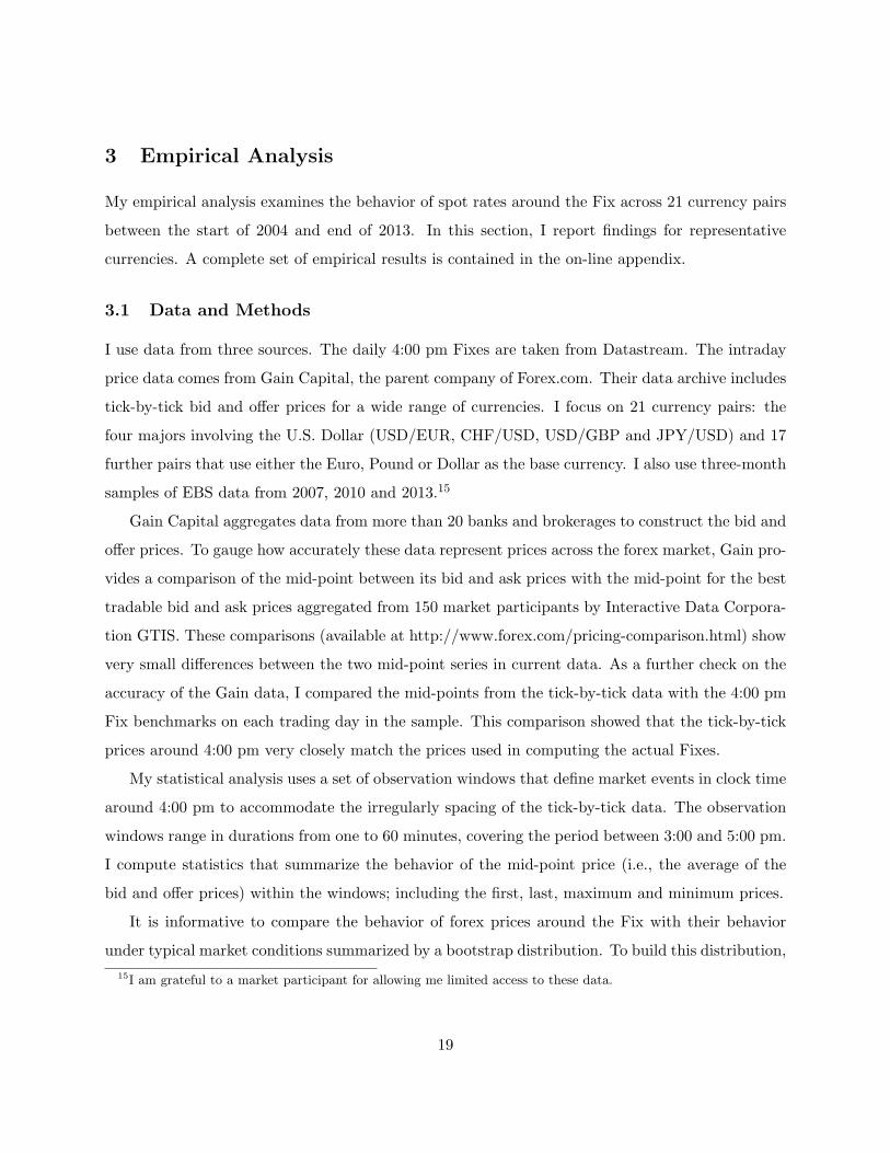
To begin my empirical analysis, I examine forex price-changes in the hour before the Fix. Figure
3 shows the densities for changes in the EUR/USD rate over horizons of 60, 15, 5, and one minute
before 4:00 pm on intra-month and end-of-month days, and the price-change density for the same
horizons from the bootstrap. The plots display two features that are common across all the 21
currency pairs. First, the behavior of pre-Fix rate changes is quite unlike the changes associated
with normal trading activity. The estimated densities for the pre-Fix changes are quite different
from the bootstrap densities. This visual evidence is confirmed by Kolmogorov-Smirnov (KS) tests
for the equality of the two distributions; they give very small p-values for all currency pairs and
horizons.16 Second, the behavior of pre-Fix rate changes at the end of the month appears more
atypical than those on other days. More specifically, the dispersion of pre-Fix rate changes at the
end of the month is significantly larger than the dispersion in the bootstrap distribution and the
dispersion of pre-Fix changes during the month. These differences are more pronounced at shorter
horizons (particularly below 15 minutes). Recall from Section 1 that there is a strong hedging
incentive for fund managers to submit Fix orders at the end of the month. The density plots
indicate that this institutional factor affects the behavior of forex prices before the Fix.
16Two versions of the KS test can be found in the statistics literature. The one-sample KS test is a nonparametrictest of the null hypothesis that the population CDF of the data is equal to the hypothesized CDF. The two-sampleKS test is a nonparametric hypothesis test of the null that the data in two samples are from the same continuousdistribution. Here I compute the two-sample KS test which uses the maximum absolute difference between the CDFs
of the distributions of the two data samples. The test statistic is computed as D = maxx
|F1(x)− F2(x)|
where
F1(x) is the proportion of the first data sample less than or equal to x, and F2(x) is the proportion of the seconddata sample less than or equal to x. The KS test and its asymptotic p-value are computed with the Matlab “kstest2”function.
20
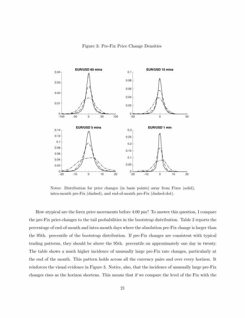
Figure 3: Pre-Fix Price Change Densities
-100 -50 0 50 100
0
0.01
0.02
0.03
0.04EUR/USD 60 mins
-50 0 50
0
0.02
0.04
0.06
0.08
0.1EUR/USD 15 mins
-20 -10 0 10 20
0
0.02
0.04
0.06
0.08
0.1
0.12
0.14EUR/USD 5 mins
-20 -10 0 10 20
0
0.05
0.1
0.15
0.2
0.25
0.3EUR/USD 1 min
Notes: Distribution for price changes (in basis points) away from Fixes (solid),
intra-month pre-Fix (dashed), and end-of-month pre-Fix (dashed-dot).
How atypical are the forex price movements before 4:00 pm? To answer this question, I compare
the pre-Fix price-changes to the tail probabilities in the bootstrap distribution. Table 2 reports the
percentage of end-of-month and intra-month days where the absolution pre-Fix change is larger than
the 95th. percentile of the bootstrap distribution. If pre-Fix changes are consistent with typical
trading patterns, they should be above the 95th. percentile on approximately one day in twenty.
The table shows a much higher incidence of unusually large pre-Fix rate changes, particularly at
the end of the month. This pattern holds across all the currency pairs and over every horizon. It
reinforces the visual evidence in Figure 3. Notice, also, that the incidence of unusually large pre-Fix
changes rises as the horizon shortens. This means that if we compare the level of the Fix with the
21

level of rates in the prior 30 minutes on a randomly chosen day, we are likely to see an unusually
large jump in rates shortly before 4:00 pm.
Table 2: Tail Probabilities for pre-Fix Price Changes
I: End-of-month II: Intra-Month
horizon 30 15 5 1 30 15 5 1(ii) (iii) (v) (vi) (ii) (iii) (v) (vi)
A: EUR/USD 22.222 18.803 22.222 33.333 11.653 9.380 7.107 10.496CHF/USD 21.698 21.698 25.472 37.736 13.242 10.939 9.433 14.969JPY/USD 28.846 38.462 47.115 61.539 12.114 11.071 10.799 22.051USD/GBP 27.586 29.310 33.621 51.724 10.822 9.665 11.276 20.446
B: CHF/EUR 23.276 25.862 29.310 33.621 9.987 9.819 11.589 15.086JPY/EUR 28.205 29.915 42.735 52.137 10.574 8.013 10.905 15.572NOK/EUR 29.032 24.194 35.484 58.065 14.330 14.562 19.597 29.202NZD/EUR 30.882 29.412 41.177 48.529 16.549 15.559 20.368 27.581SEK/EUR 25.424 30.509 45.763 45.763 13.975 16.149 15.450 29.115
C: AUS/GBP 30.435 34.783 34.783 56.522 12.940 13.008 14.160 26.423CAD/GBP 28.169 30.986 38.028 39.437 14.614 16.238 22.463 30.176CHF/GBP 30.172 37.069 31.035 50.000 10.923 11.378 12.743 21.804EUR/GBP 31.304 40.000 37.391 50.435 10.603 12.399 12.185 22.488JPY/GBP 27.586 32.759 43.966 56.035 10.132 10.008 11.373 21.464NZD/GBP 25.373 25.373 26.866 47.761 13.272 12.420 21.221 30.518
D: AUS/USD 28.448 23.276 32.759 46.552 12.427 11.259 13.136 19.516CAD/USD 31.897 29.310 34.483 43.966 16.722 15.183 16.889 26.040DKK/USD 15.254 10.170 18.644 30.509 10.881 6.820 7.126 10.575NOK/USD 22.581 19.355 29.032 46.774 12.481 9.954 12.864 24.043SEK/USD 20.339 23.729 33.898 40.678 12.336 11.334 11.411 22.282SGD/USD 11.475 9.836 16.393 19.672 9.667 8.917 10.083 18.667
Notes: Each cell reports the percentage of days in which the absolute basis point change in prices in the window before the
Fix is larger than the 95th. percentile from the bootstrap distribution of absolute basis point price changes away from the
Fix. Panel I reports the percentage for end-of-month price changes, panel II the percentage for intra-month price changes.
Examples of large forex price movements immediately before 4:00 pm on particular days for
specific currencies have been reported by Vaugham and Finch (2013), Melvin and Prins (2015)
and others. The statistics in Table 2 show that unusually large pre-Fix price changes are almost
commonplace. For example, atypically large changes in the minute before the Fix on intra-month
22

days occur at more than three times the rate that would be consistent with normal trading activity
across the four major currency pairs, and at higher rates across the other currency pairs. The
incidence of atypically large price changes immediately before the Fix is even higher at the end
of the month. At the one-minute horizon, atypical changes occur between four and twelve times
the rate consistent with normal trading activity. These are remarkably high numbers. For two of
the major currency pairs (JPY/USD and USD/GBP) atypically large price changes in the minute
before 4:00 pm occur at more than ten times the rate consistent with normal trading activity.
It is also informative to examine the incidence of atypically large pre-Fix price changes through
time. For this purpose Table 3 reports the number of atypical changes (again using the 95th.
percentile threshold) over a one-minute horizon at the end of the month for each year covered by
the dataset. P-values for the null hypothesis that the number of atypical end-of-month changes
occurs by chance (based on the bootstrap distribution) are reported in parenthesis. As the table
clearly shows, the high incidence of atypically large pre-Fix price changes is not concentrated in
a few years or currency pairs. On the contrary, it is pervasive. For example, in the USD/GBP
case, there have been a high number of atypically large changes in every year between 2004 and
2013. In fact, the numbers are so high in nine of the years that the probability of this representing
normal price movements in USD/GBP in any year is less than 0.001 (i.e., less that one in one
thousand). This repeated high incidence of atypically large pre-Fix price changes is also evident
in the JPY/USD, JPY/EUR, CHF/GBP, EUR/GBP, JPY/GBP, USD/USD and CAD/USD. The
results in Table 3 also show that the peak incidence of atypically large rate changes did not occur
around the world financial crisis. Aggregating across all 21 currency pairs, the peak year was 2010
with a total of 148.
23

Table 3: Pre-Fix Tail Events By Year (1 minute window)
2004 2005 2006 2007 2008 2009 2010 2011 2012 2013
A: EUR/USD 2 5 1 6 5 6 6 3 4 2(0.165) (0.000) (0.600) (0.000) (0.000) (0.000) (0.000) (0.028) (0.003) (0.138)
CHF/USD 1 4 0 5 3 4 5 7 7 4(0.450) (0.001) (0.569) (0.000) (0.007) (0.002) (0.000) (0.000) (0.000) (0.002)
JPY/USD 3 4 7 11 5 6 9 8 4 7(0.011) (0.001) (0.000) (0.000) (0.000) (0.000) (0.000) (0.000) (0.003) (0.000)
USD/GBP 6 5 6 3 5 9 7 8 5 7(0.000) (0.000) (0.000) (0.028) (0.000) (0.000) (0.000) (0.000) (0.000) (0.000)
B: CHF/EUR 4 1 1 3 4 4 9 7 0 6(0.003) (0.550) (0.550) (0.028) (0.003) (0.003) (0.000) (0.000) (0.540) (0.000)
JPY/EUR 6 4 4 7 8 8 9 5 5 5(0.000) (0.002) (0.002) (0.000) (0.000) (0.000) (0.000) (0.000) (0.000) (0.000)
NOK/EUR 1 8 8 10 6 4(0.200) (0.000) (0.000) (0.000) (0.000) (0.002)
NZD/EUR 8 7 5 4 5 4(0.000) (0.000) (0.000) (0.003) (0.000) (0.002)
SEK/EUR 1 4 7 6 5 6(0.200) (0.003) (0.000) (0.000) (0.000) (0.000)
C: AUS/GBP 10 9 8 6 5 2(0.000) (0.000) (0.000) (0.000) (0.000) (0.138)
CAD/GBP 6 5 6 4 4 3(0.000) (0.000) (0.000) (0.003) (0.003) (0.021)
CHF/GBP 4 3 4 5 7 7 8 7 7 7(0.003) (0.021) (0.002) (0.000) (0.000) (0.000) (0.000) (0.000) (0.000) (0.000)
EUR/GBP 3 3 4 4 7 8 9 7 8 6(0.028) (0.021) (0.002) (0.003) (0.000) (0.000) (0.000) (0.000) (0.000) (0.000)
JPY/GBP 4 3 4 8 7 9 10 6 6 9(0.003) (0.021) (0.002) (0.000) (0.000) (0.000) (0.000) (0.000) (0.000) (0.000)
NZD/GBP 6 8 7 6 4 2(0.000) (0.000) (0.000) (0.000) (0.003) (0.138)
D: AUS/USD 4 3 5 4 9 9 9 4 3 4(0.002) (0.021) (0.000) (0.003) (0.000) (0.000) (0.000) (0.003) (0.028) (0.002)
CAD/USD 4 3 5 7 6 5 4 3 7 8(0.003) (0.021) (0.000) (0.000) (0.000) (0.000) (0.003) (0.028) (0.000) (0.000)
DKK/USD 3 5 6 2 1 2(0.001) (0.000) (0.000) (0.165) (0.600) (0.138)
NOK/USD 2 8 6 6 4 4(0.015) (0.000) (0.000) (0.000) (0.003) (0.002)
SEK/USD 3 3 7 5 3 5(0.001) (0.021) (0.000) (0.000) (0.028) (0.000)
SGD/USD 2 3 3 1 1 2(0.015) (0.028) (0.028) (0.600) (0.600) (0.138)
Notes: Each cell reports the number of months in each year where the absolute change in prices in the one minute before the
Fix falls in the 95th percentile of the bootstrap distribution of price changes away from the Fix. P-values for the null that
the number of months occurs purely by chance are reported in parentheses. Empty cells signify the absence of data for the
currency pair in that year.
24

These findings extend the volatility results in Melvin and Prins (2015). They showed that on
average across currencies, volatility rises in the hour before the Fix at the end of the month. Here
we see that changes in forex prices observed immediately before the 4:00 pm Fix are extraordinarily
unusual when compared to their behavior in normal trading away from the Fix: prices regularly
jump by an amount that is very rarely seen elsewhere. Moreover, the incidence of these atypically
large pre-Fix price changes is particularly high at the end of each month, appears pervasive across
all the currency pairs and throughout the sample period.
3.3 Post-Fix Prices
The high incidence of unusually large changes in prices immediately before the Fixes carries over into
the behavior of prices after 4:00 pm. Table 4 reports the incidence of large post-Fix price changes
(starting at 4:00 pm) over horizons of one to 30 minutes. As above, I use the 95th. percentile
threshold from the bootstrap distribution to identify atypically large price changes, and report
their incidence for individual currency pairs at the end of each month and on other intra-month
days. As the table shows, the incidence of atypically large changes on intra-month days is almost
twice the rate we would expect to see in trading away from the Fix for many of the currency pairs.
The incidence of unusually large price changes is much higher at the end of the month. For most
currency pairs, the incidence at the one-minute horizon is at least four times higher than we would
expect to see in normal trading, declining to between two and three times normal at the 30-minute
horizon. While high, these incidence rates are well below those reported for pre-Fix price changes
in Table 2 over comparable horizons.
25

Table 4: Tail Probabilities for Post-Fix Price Changes
I: End-of-Month II: Intra-Month
horizon 30 15 5 1 30 15 5 1(ii) (iii) (v) (vi) (ii) (iii) (v) (vi)
A: EUR/USD 14.530 15.385 17.094 20.513 9.711 9.298 8.554 6.157CHF/USD 15.094 18.868 18.868 26.415 9.965 9.699 8.193 6.997JPY/USD 18.269 16.346 21.154 21.154 8.439 8.893 8.394 9.483USD/GBP 15.517 14.655 13.793 18.103 8.137 7.228 8.922 6.939
B: CHF/EUR 10.345 16.379 19.828 16.379 8.681 7.965 8.681 8.260JPY/EUR 12.821 16.239 18.803 25.641 8.468 7.600 8.798 7.435NOK/EUR 8.065 4.839 12.903 20.968 7.591 6.739 10.380 18.048NZD/EUR 22.059 16.177 26.471 41.177 8.911 7.638 10.113 11.245SEK/EUR 11.864 13.559 16.949 40.678 7.531 7.609 8.385 16.537
C: AUS/GBP 20.290 23.188 28.986 26.087 7.859 6.911 7.114 8.537CAD/GBP 19.718 19.718 33.803 23.944 7.375 7.510 8.660 8.187CHF/GBP 11.207 14.655 20.690 21.552 7.199 7.613 8.440 9.102EUR/GBP 14.783 19.130 19.130 26.087 6.156 6.841 7.738 10.389JPY/GBP 11.207 15.517 15.517 14.655 7.568 8.189 8.519 7.610NZD/GBP 20.896 13.433 32.836 31.343 7.239 6.529 9.226 11.001
D: AUS/USD 10.345 18.103 27.586 24.138 9.425 8.674 9.008 7.381CAD/USD 18.103 17.241 30.172 30.172 9.942 9.318 10.399 9.193DKK/USD 11.864 10.170 15.254 18.644 8.736 9.042 8.429 5.900NOK/USD 14.516 14.516 22.581 24.194 8.959 8.499 8.116 11.792SEK/USD 16.949 11.864 18.644 28.814 8.790 8.867 7.941 11.103SGD/USD 4.918 3.279 8.197 27.869 7.167 7.917 7.667 14.667
Notes: Each cell reports the percentage of days in which the absolute basis point change in prices in the window after the
Fix is larger than the 95 percentile from the bootstrap distribution. Panel I reports the percentage for end-of-month price
changes, panel II the percentage for intra-month price changes.
26

Figure 4: Bivariate Pre- and Post- Fix Price Change Densities
pre
post
EUR/USD 15 mins
−40 −20 0 20 40−40
−20
0
20
40
pre
post
EUR/USD 10 mins
−20 −10 0 10 20−20
−10
0
10
20
pre
post
EUR/USD 5 mins
−20 −10 0 10 20−20
−10
0
10
20
pre
post
EUR/USD 1 mins
−10 −5 0 5 10−10
−5
0
5
10
Notes: Each plot shows the contours of the estimated bivariate density for pre- and post-Fix price
changes (in basis points) over horizons of 1 to 15 minutes. The solid line in each plot is the estimated
regression line from the regression on the post-Fix change in the pre-Fix change. All estimates are
based on end-of-month data.
The statistics in Tables 2 and 4 clearly establish that forex prices are unusually volatile imme-
diately before and after the Fix, particularly at the end of the month. I now consider how the pre-
and post-Fix behavior of prices are linked. For this purpose, I estimate the bivariate density for
pre- and post-Fix price changes g(ln(St+h/Sfixt ), ln(Sfix
t /Sth)) at different horizons, h.17 Figure
4 shows a contour plot of estimated density for the EUR/USD in end-of-month data at different
horizons. The solid line shows the projection (i.e. regression) of ln(St+h/Sfixt ) on ln(Sfix
t /Sth).
This splits the post-Fix price change into a portion that is perfectly correlated with the pre-Fix
17Estimation uses a Gaussian Kernel with the bandwidth determined as in Bowman and Azzalini (1997).
27

change, the projection P(ln(Sfixt /Sth)); and a projection error, ηt+h, that is uncorrelated with
the pre-Fix change:
ln(St+h/Sfixt ) = P(ln(Sfix
t /Sth)) + ηt+h.
Several features of the EUR/USD plots in Figure 4 appear across all the currency pairs. First,
the maximum width of each contour exceeds its maximum height because prices are more volatile
immediately before than after the Fix. Second, the contours generally appear as ellipses that are
rotated clockwise around the point (0,0). This pattern implies that positive post-Fix price changes
are more likely than negative changes if they were preceded by a negative pre-Fix change and vise-
verse. Third, the projection lines slope downwards (from left to right) at all horizons and across
all currency pairs.
Table 5 reports the estimated projection coefficients, their (heteroskedastic-consistent) standard
errors, and the uncentered R2 statistics for the projections over the horizons of 1, 5, and 15
minutes. The estimated coefficients are uniformly negative, ranging in value from -0.07 to -0.61.
They are statistically significant at the five percent level for all but three currencies (EUR/USD,
CHF/USD and CAD/GBP) for at least one horizon. The R2 statistics measure the variance
contribution of the projections to the post-Fix price changes. As the table shows, these statistics are
generally small (i.e. below 0.2). This indicates that most of the variation in post-Fix changes over
time is attributable to projection errors that are uncorrelated with the pre-Fix changes. Notable
exceptions to this pattern include the NZD/GBP, AUD/GBP, NZD/EUR and JPY/EUR, where
the R2 statistics are a good deal larger. In these currencies, price reversion accounts for a significant
fraction of the time series variation in post-Fix price changes.
In summary, forex prices display an unusually high level of volatility in the minutes immediately
following 4:00 pm. They also appear to be influenced by the pre-Fix behavior of prices: Over a wide
range of currencies and horizons, there is a statistically significant negative correlation between pre-
and post-Fix price changes.
28

Table 5: Post-Fix Projection Estimates
15 Minutes 5 Minutes 1 Minute
Coeff Std Error R2 Coeff Std Error R2 Coeff Std Error R2
A: EUR/USD -0.129 (0.077) 0.018 -0.251 (0.165) 0.060 -0.150 (0.082) 0.048CHF/USD -0.107 (0.150) 0.009 -0.112 (0.209) 0.015 -0.160 (0.138) 0.035JPY/USD -0.081 (0.090) 0.011 -0.126 (0.068) 0.051 -0.164 (0.045) 0.173USD/GBP -0.201 (0.118) 0.115 -0.357 (0.255) 0.243 -0.105 (0.046) 0.066
B: CHF/EUR -0.235 (0.078) 0.113 -0.199 (0.107) 0.104 -0.096 (0.129) 0.020JPY/EUR -0.375 (0.154) 0.257 -0.467 (0.168) 0.408 -0.605 (0.200) 0.633NOK/EUR -0.167 (0.073) 0.089 -0.211 (0.049) 0.162 -0.075 (0.110) 0.009NZD/EUR -0.309 (0.077) 0.307 -0.439 (0.126) 0.447 -0.141 (0.118) 0.061SEK/EUR -0.233 (0.061) 0.209 -0.410 (0.107) 0.307 -0.199 (0.070) 0.068
C: AUD/GBP -0.303 (0.042) 0.377 -0.431 (0.050) 0.464 -0.031 (0.050) 0.008CAD/GBP -0.038 (0.130) 0.002 -0.344 (0.260) 0.079 -0.040 (0.103) 0.003CHF/GBP -0.267 (0.108) 0.161 -0.410 (0.180) 0.298 -0.150 (0.085) 0.079EUR/GBP -0.228 (0.097) 0.134 -0.473 (0.185) 0.365 -0.209 (0.047) 0.168JPY/GBP -0.147 (0.145) 0.066 -0.256 (0.223) 0.149 -0.155 (0.039) 0.179NZD/GBP -0.397 (0.049) 0.536 -0.505 (0.053) 0.633 -0.246 (0.075) 0.239
D: AUD/USD -0.247 (0.056) 0.170 -0.256 (0.106) 0.144 -0.124 (0.080) 0.061CAD/USD -0.189 (0.074) 0.069 -0.315 (0.052) 0.140 -0.178 (0.064) 0.071DKK/USD -0.259 (0.108) 0.054 -0.312 (0.255) 0.079 -0.164 (0.102) 0.065NOK/USD -0.135 (0.085) 0.029 -0.169 (0.089) 0.043 -0.079 (0.086) 0.014SEK/USD -0.237 (0.102) 0.111 -0.396 (0.159) 0.161 -0.234 (0.068) 0.126SGD/USD -0.443 (0.238) 0.212 -0.313 (0.161) 0.156 -0.154 (0.309) 0.015
Notes: The table reports the estimated projection coefficient, its (heteroskedastic consistent) standard error, and the R2 statistic from the
projection of the post-Fix price change on the pre-Fix change over the horizons shown at the top of each panel. The “∗” indicates statistical
significance at the 5 percent level.
29

4 Economic Perspective
This section provides an economic perspective on my empirical results. First, I examine the impli-
cations of the negative correlation between pre- and post-Fix price changes for average price paths
around the Fix. I then investigate whether this correlation could have supported the presence of
attractive and exploitable trading opportunity to market participants at the time. Finally, I con-
sider my results in context of the reports issued of U.K. Financial Conduct Authority and the U.S.
Department of Justice.
4.1 Average Price Paths
The projection results in Table 5 show the existence of a strong statistical link between pre- and
post-Fix price changes. Figure 5 provides another perspective on the temporal dependence in forex
prices. Here I plot the average price paths for the major currency pairs around the Fix conditioned
on the pre-Fix price change. The vertical axis shows basis points relative to the price at 3:45 pm
while the horizontal axis shows minutes relative to 4:00 pm. Each panel shows six average paths
that are conditioned on the change in prices between 3:45 and 4:00 pm. I condition on this horizon
because 3:45 pm is the cut-off time for dealer-banks to accept Fix orders. The solid black lines in
each plot depict the average path across all end-of-month trading days. Average paths for intra-
month days are shown by dashed lines. The remaining upper and lower lines (drawn with dashes
and dots) identify the average paths on end-of-the-month trading days where the pre-Fix price
change is in the 75th. and 25th. percentiles of the pre-Fix price-change distribution, respectively.
30

Figure 5: Rate Paths Around the Fix
-60 -45 -30 -15 0 15 30 45 60
-15
-10
-5
0
5
10
15
EUR/USD
-60 -45 -30 -15 0 15 30 45 60
-20
-15
-10
-5
0
5
10
15
20
CHF/USD
-60 -45 -30 -15 0 15 30 45 60
-20
-15
-10
-5
0
5
10
15
20
JPY/USD
-60 -45 -30 -15 0 15 30 45 60
-25
-20
-15
-10
-5
0
5
10
15
20
25USD/GBP
Notes: Average rate path in basis points around 3:45 pm level conditioned on: (i) pre-Fix changes (over 15 mins) at end of month
(solid black); (ii) pre-Fix changes above the 75th. percentile of end-of-month distribution (dashed dot); (iii) pre-Fix changes in the
25th. percentile of end-of-month distribution (dashed dot); (iv) positive and negative pre-Fix changes on intra-month days (dashed).
For the sake of clarity, both the dotted and dash-dotted lines are hidden to the left of -15.
There are several noteworthy features in Figure 5 that are present in the plots for the other
currencies (see Appendix). First, consider the paths on intra-month days. These paths identify very
small reversals during the first minute after the Fix (on the order of one basis point). Thereafter,
the paths are almost flat for all the currency pairs. These patterns imply that all the relevant
trade-based information is fully assimilated into prices by the end of the Fix window, so there is
no systematic tendency for rates to rise or fall after that. In this sense, it appears that post-Fix
equilibrium prices are quickly established on intra-month trading days.
The price paths from end-of-month trading days are quite different. Consistent with the statis-
31

tics on pre-Fix rate volatility, changes in prices between 3:45 and 4:00 pm are larger (in absolute
value). Prices also tend to move in a systematic pattern after 4:00 pm. The plots for many of
the currencies show that both positive and negative pre-Fix price changes are followed by a sizable
reversal in prices in the first few minutes (see, e.g., AUD/GBP, AUD/USD, and NZD/EUR). Fig-
ure 5 shows that for other currencies (see, e.g., JYP/USD and USD/GDP) the reversals are larger
following pre-Fix rate changes in one direction. These asymmetric effects were not captured by the
projection results in Table 5. Figure 5 also shows that large pre-Fix price changes are followed by
bigger price reversals than on average across all end-of-month trading days for some currency pairs
(see, e.g., CHF/USD).
One further feature of these plots deserves note. All the plotted price paths are conditioned on
the change in prices between 3:45 and 4:00 pm without regard to when prices changed during that
15-minute window. Thus, if most of the movement in prices occurred immediately before or at the
start of the Fix window, the paths would be flat until a point just to the left of the vertical line.
Instead, the paths for all the currencies show that on average prices start “drifting” upwards or
downwards soon after 3:45 pm. In other words, the actions of market participants start a process
that moves prices towards the Fix benchmark well before 4:00 pm on both intra- and end-of-month
trading days. I discuss this feature of the data further below.
4.2 Trading Around the Fix
The projection results in Table 5 and price paths in Figure 5 suggest that a simple end-of-month
trading strategy of taking a long (short) position at 4:00 pm if prices fell (rose) towards the Fix
should generate positive returns on average. Would such a strategy be attractive to a sophisticated
trader who has access to the best bid and ask prices in the market?
To address this question, I computed the realized returns R on trading strategies that initiated
long and short positions at the end-of-month Fixes with durations of h = 1, 5, 15 minutes. The
long and short positions are selected according to the price changes over the h minutes before
4:00 pm. I assume that the benchmark well-approximates the transaction price that sophisticated
traders actually face when initiating a position at 4:00 pm because spreads fall during the Fix
window. Thereafter, for the next hour or so, spreads return to their normal level. So I assume
that a trader closing out a position faces bid (ask) prices equal to the mid-point price minus (plus)
32

one-half the normal spread computed from my 2013 sample of EBS data.18
I compute three performance measures to assess the attractiveness of the strategies: (i) the
average return, (ii) the Sharpe Ratio and (iii) the Maximum Drawdown. The Sharpe Ratio is
calculated as SR = 1p252
(ET [Ri]− 1) /p
VT [Ri], where Ri is the (gross) return on day i. ET [.]
and VT [.] are the sample mean and variance from the T returns computed over the span of the
data. Because returns are generated at the daily frequency, I include the 1/√252 scale factor to
“annualize” the ratio (using the convention that a year equals 252 trading days). Sharpe Ratios are
widely used by financial market participants to judge the attractiveness of trading strategies. The
Maximum Drawdown statistic is another widely-used measure. It is computed as the maximum
percentage drop (i.e. from peak to trough) in the cumulated return from following the trading
strategy over the span of data. As such, it provides a measure of downside risk.
Table 6 reports the performance measures for the end-of-month trading strategies across all
the currency pairs. Columns (i) - (iii) show that average returns are positive for the majority
of currencies and horizons. In fact, the returns are positive for at least one horizon in all but
the JPY/USD and USD/GBP. Furthermore, the average returns are well over five percent (on an
annualized basis) for nine currency pairs at some horizons. The strategies for many currency pairs
also appear attractive when judged by the Sharpe Ratios and Drawdown Statistics. The ratios are
above one for at least one horizon in 15 of the currency pairs, and over two in eight pairs. These
ratios are well above the minimum thresholds required by financial institutions before they will
allocate capital to a trading strategy (see, Lyons, 2001), and they exceed the ratios computed for
carry trades (see, Burnside, 2012). The downside risk associated with the strategies is also generally
low with most of the Drawdown statistics below two percent. Overall, these statistics show that
the trading strategies in many currency pairs appear economically attractive ex-post (i.e., looking
back over the sample period).
18While the Gain data accurately measures the mid-point between the best tradable prices available to retail tradingplatforms, the spread between Gain’s bid and ask prices is roughly twice as large as the inside spreads between thebest bid and ask prices on interbank trading venues run by EBS and Reuters. Sophisticated traders, such as hedgefund managers, can trade on these interbank venues via prime brokerage accounts, so I use these inside spreads fromEBS to estimate the transaction prices these traders face. For example, in the case where the price falls before theFix, the strategy requires taking a long position at the Fix, so the return is computed as ln(St+h −
1
2δ) − lnSfix
t ,where δ is the average EBS inside spread each minute (excluding the Fix window) between 7:00 am and 5:00 pm.Similarly, in cases where the price rises before the Fix, the return is lnSfix
t − ln(St+h + 1
2δ).
33
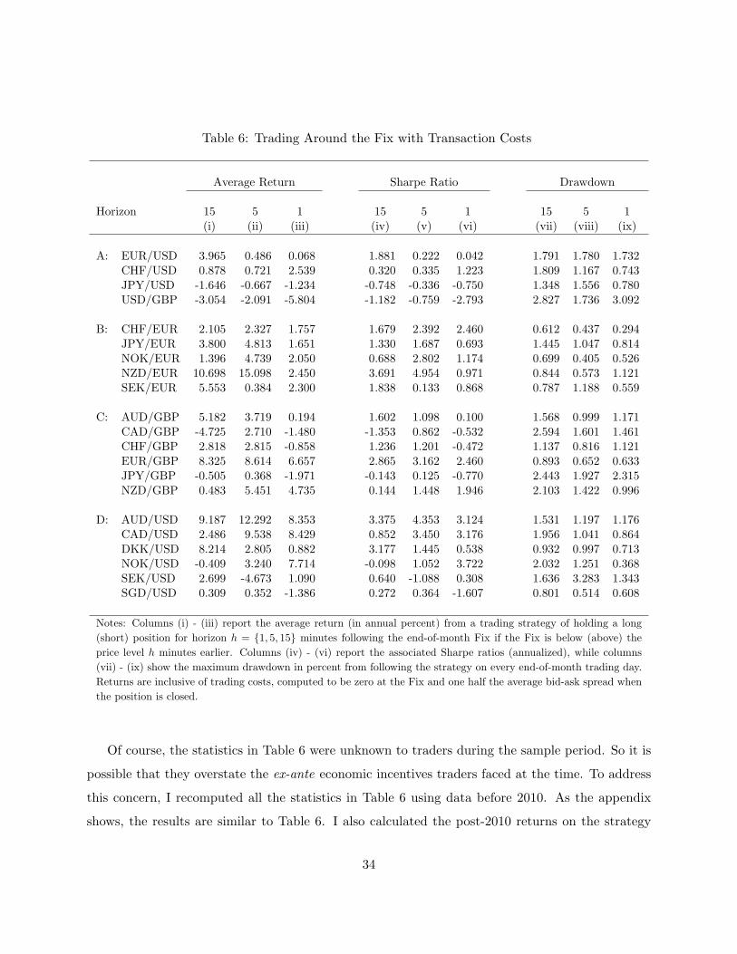
Table 6: Trading Around the Fix with Transaction Costs
Average Return Sharpe Ratio Drawdown
Horizon 15 5 1 15 5 1 15 5 1(i) (ii) (iii) (iv) (v) (vi) (vii) (viii) (ix)
A: EUR/USD 3.965 0.486 0.068 1.881 0.222 0.042 1.791 1.780 1.732CHF/USD 0.878 0.721 2.539 0.320 0.335 1.223 1.809 1.167 0.743JPY/USD -1.646 -0.667 -1.234 -0.748 -0.336 -0.750 1.348 1.556 0.780USD/GBP -3.054 -2.091 -5.804 -1.182 -0.759 -2.793 2.827 1.736 3.092
B: CHF/EUR 2.105 2.327 1.757 1.679 2.392 2.460 0.612 0.437 0.294JPY/EUR 3.800 4.813 1.651 1.330 1.687 0.693 1.445 1.047 0.814NOK/EUR 1.396 4.739 2.050 0.688 2.802 1.174 0.699 0.405 0.526NZD/EUR 10.698 15.098 2.450 3.691 4.954 0.971 0.844 0.573 1.121SEK/EUR 5.553 0.384 2.300 1.838 0.133 0.868 0.787 1.188 0.559
C: AUD/GBP 5.182 3.719 0.194 1.602 1.098 0.100 1.568 0.999 1.171CAD/GBP -4.725 2.710 -1.480 -1.353 0.862 -0.532 2.594 1.601 1.461CHF/GBP 2.818 2.815 -0.858 1.236 1.201 -0.472 1.137 0.816 1.121EUR/GBP 8.325 8.614 6.657 2.865 3.162 2.460 0.893 0.652 0.633JPY/GBP -0.505 0.368 -1.971 -0.143 0.125 -0.770 2.443 1.927 2.315NZD/GBP 0.483 5.451 4.735 0.144 1.448 1.946 2.103 1.422 0.996
D: AUD/USD 9.187 12.292 8.353 3.375 4.353 3.124 1.531 1.197 1.176CAD/USD 2.486 9.538 8.429 0.852 3.450 3.176 1.956 1.041 0.864DKK/USD 8.214 2.805 0.882 3.177 1.445 0.538 0.932 0.997 0.713NOK/USD -0.409 3.240 7.714 -0.098 1.052 3.722 2.032 1.251 0.368SEK/USD 2.699 -4.673 1.090 0.640 -1.088 0.308 1.636 3.283 1.343SGD/USD 0.309 0.352 -1.386 0.272 0.364 -1.607 0.801 0.514 0.608
Notes: Columns (i) - (iii) report the average return (in annual percent) from a trading strategy of holding a long
(short) position for horizon h = 1, 5, 15 minutes following the end-of-month Fix if the Fix is below (above) the
price level h minutes earlier. Columns (iv) - (vi) report the associated Sharpe ratios (annualized), while columns
(vii) - (ix) show the maximum drawdown in percent from following the strategy on every end-of-month trading day.
Returns are inclusive of trading costs, computed to be zero at the Fix and one half the average bid-ask spread when
the position is closed.
Of course, the statistics in Table 6 were unknown to traders during the sample period. So it is
possible that they overstate the ex-ante economic incentives traders faced at the time. To address
this concern, I recomputed all the statistics in Table 6 using data before 2010. As the appendix
shows, the results are similar to Table 6. I also calculated the post-2010 returns on the strategy
34

for each currency pair that had the highest Sharpe Ratio in the pre-2010 data. This produced an
average return across the currencies of 3.25 percent. Consistent with this experimental evidence,
industry newsletters during the sample period discussed the attractiveness of trading around end-
of-month fixes (see, Credit Suisse, 2009). Taken together, these findings suggest the existence of
significant ex-ante incentives for traders to exploit the temporal pattern in forex prices around
end-of-month Fixes.
4.3 Competition and Collusion
Banks view their trading data as highly proprietary, and as such have not made this data available
to researchers. Consequently, it is impossible to directly examine whether the collusive activity
described by the U.K. Financial Conduct Authority and the U.S. Department of Justice can actually
account for the behavior of forex prices around the Fix presented above.19 Nevertheless, there are
two strands of indirect evidence that shed light on this issue.
The first strand comes from the model of competitive forex trading in Section 2. Recall that
Fix orders only contribute to the volatility in equilibrium prices when they are filled by dealers
during round f. This theoretical prediction is consistent with the empirical evidence on post-Fix
price changes in Table 4. By contrast, the model cannot account for the volatility in pre-Fix
prices shown in Tables 2 and 3. Nor can it explain the negative correlation between pre- and
post-Fix changes documented in Table 5 and depicted in Figure 4. The most likely source of these
inconsistencies concerns the information available to dealers in the model. If contrary to the model’s
assumptions, dealers had the opportunity to share information about their individual Fix orders
before quoting prices in round ii, they would find it beneficial to do so. Moreover, the aggregate
imbalance in Fix orders would become known to all dealers as a result of this information sharing
and would be incorporated into their price quotes to efficiently share risk. In this alternate collusive
equilibrium, the aggregate imbalance in Fix orders would impact forex prices before the Fix; which
would be more consistent with the empirical results in Tables 2 and 3. This is indirect evidence
suggesting that the sharing of information about Fix orders could have played a role in determining
the empirical behavior of forex prices before the Fix.
19The reports provide examples of collusive activity by individual bank dealers, but they do not contain anysystematic analysis of how these activities affected forex prices across the market. The on-line appendix gives furtherdetails concerning these reports and the settlements reached by the banks.
35

Regulators’ investigation reports contain the second strand of evidence. According to the U.K.
Financial Conduct Authority and the U.S. Department of Justice, the dealers shared information
about their Fix orders around 3:45 pm and colluded to front run their joint imbalance in orders
prior to the start of the Fix window. That is to say, the dealers would purchase forex before the Fix
window when they collectively had net orders to buy, and sell forex before the Fix window when
they collectively had net orders to sell. The dealers also traded among themselves to concentrate
the net order imbalance at one or two trading desks. Dealers at these desks would then attempt
to manipulate the Fix by aggressively trading in the interbank market (on EBS or Reuters) once
the Fix window opened. This typically involved placing a large number of market purchase orders
when they had net orders to buy forex, and market sale orders when they had net orders to sell
forex (during the first 30 seconds of the window). Trading in this manner increased the likelihood
that the Fix would move in the desired direction because the WMR methodology took no account
of trading volume. After successfully manipulating the Fix by this means, the colluding dealers
would close out the speculative positions they established before the Fix window at a profit.
The market-wide effects of these activities depend critically on whether the imbalance in Fix
orders across all the colluding dealers was in the same direction as the imbalance across the entire
market. In cases where the imbalances are in the same direction, we would expect to see patterns
like those in Figure 5. In particular, the anticipatory movements in forex prices soon after 3:45
pm is consistent with colluding dealers establishing speculative positions by front running, while
the reversal of prices after 4:00 pm is consistent with colluding dealers closing these positions after
the Fix. In addition, aggressive trading within the Fix window by some colluding dealers would
add to volatility in spot rates due to the market-wide imbalance in Fix orders, consistent with the
volatility results in Tables 2-4.
The presence of collusion also provides a simple potential explanation for the existence of
economically attractive trading strategies exploiting the negative serial correlation in price changes
around the Fix. Normally, we would expect these temporal patterns in prices to disappear soon
after they are discovered as traders attempted to exploit them. However, the results in Table 6
suggest that here the actions of some market participants impeded this process. The regulators’
descriptions of the collusive front running by dealers could have played this role.
36

5 Conclusion
This paper has examined the behavior of forex prices around the WRM Fix from both a theoretical
and empirical perspective. The theoretical perspective was provided by a new microstructure model
of competitive trading that incorporated the key institutional features of the Fix. The model showed
that Fix orders have a limited effect on the behavior of forex prices. In particular, prices adjust to
the aggregate imbalance in Fix orders across the market when dealers trade to fill their individual
Fix orders. They do not contribute to the behavior of prices before the Fix nor are they a source
of serial correlation in price changes around the Fix.
My empirical results provide a different perspective. They show that across all time periods
and currency pairs changes in prices before and after the Fix are regularly of a size rarely seen in
normal trading activity. This atypical behavior is particularly strong at the end of each month.
Furthermore, the temporal dependence in forex prices around the Fix (i.e., the negative correla-
tion between pre- and post-Fix price changes) appear sufficiently strong to support economically
attractive end-of-month trading strategies for many currency pairs.
37

References
Abrantes-Metz, Rosa M., Michael Kraten, Albert D. Metz, and Gim S. Seow. 2012. “LIBOR
manipulation?” Journal of Banking and Finance 36 (1):136—150.
Allen, Franklin and Douglas Gale. 1992. “Stock-price manipulation.” Review of financial studies
5 (3):503–529.
Almgren, Robert. 2012. “Optimal trading with stochastic liquidity and volatility.” SIAM Journal
on Financial Mathematics 3 (1):163–181.
Bertsimas, Dimitris and Andrew W Lo. 1998. “Optimal control of execution costs.” Journal of
Financial Markets 1 (1):1–50.
Bjønnes, Geir H. and Dagfinn Rime. 2005. “Dealer Behavior and Trading Systems in Foreign
Exchange Markets.” Journal of Financial Economics 75 (3):571–605.
Bollerslev, Tim and Michael Melvin. 1994. “Bid-Ask Spreads and Volatility in the Foreign Exchange
Market: An Empirical Analysis.” Journal of International Economics 36:355–372.
Bowman, Adrian W and Adelchi Azzalini. 1997. Applied Smoothing Techniques for Data Analysis:
The Kernel Approach with S-Plus Illustrations: The Kernel Approach with S-Plus Illustrations.
Oxford University Press.
Burnside, Craig. 2012. Handbook of Exchange Rates, chap. Carry Trades and Risk. John Wiley &
Sons, 283–312.
Comerton-Forde, Carole and Talis J. Putnins. 2011. “Measuring closing price manipulation.”
Journal of Financial Intermediation 20 (2):135 – 158.
Cushing, David and Ananth Madhavan. 2000. “Stock returns and trading at the close.” Journal
of Financial Markets 3 (1):45 – 67.
Eisl, Alexander, Rainer Jankowitsch, and Marti G Subrahmanyam. 2014. “The manipulation
potential of Libor and Euribor.” Available at SSRN 2201013 .
38

Evans, Martin D. D. 2011. Exchange-Rate Dynamics. Princeton Series in International Finance.
Princeton University Press.
Evans, Martin D. D. and Richard K. Lyons. 2002. “Order flow and exchange rate dynamics.”
Journal of Political Economy 110 (1):170–180.
Gagnon, Joseph E et al. 2012. “Combating widespread currency manipulation.” Policy Brief in
International Economics :12–19.
Hart, Oliver D. 1977. “On the profitability of speculation.” The Quarterly Journal of Economics
:579–597.
Hendershott, Terrence and Albert J. Menkveld. 2014. “Price pressures.” Journal of Financial
Economics 114 (3):405 – 423.
Hillion, Pierre and Matti Suominen. 2004. “The manipulation of closing prices.” Journal of Finan-
cial Markets 7 (4):351 – 375.
Ito, Takatoshi, Richard K. Lyons, and Michael T. Melvin. 1998. “Is There Private Information in
the FX Market? The Tokyo Experiment.” Journal of Finance 53 (3):1111–1130.
Ito, Takatoshi and Masahiro Yamada. 2015. “Was the Forex Fixing Fixed?” Working Paper 21518,
National Bureau of Economic Research.
King, Michael R., Carol L. Osler, and Dagfinn Rime. 2013. “The market microstructure approach
to foreign exchange: Looking back and looking forward.” Journal of International Money and
Finance 38:95 – 119. 30th Anniversary of the Journal of International Money and Finance.
Levine, Matt. 2014. “Bloomberg View: Banks manipulated foreign exchange in ways you can’t
teach.” URL http://www.bloomberg.com/view/articles/2014-11-12/.
Lyons, Richard K. 1995. “Tests of Microstructural Hypothesis in the Foreign Exchange Market.”
Journal of Financial Economics 39 (2-3):321–351.
———. 1997. “A Simultaneous Trade Model of the Foreign Exchange Hot Potato.” Journal of
Financial Economics 42 (3-4):275–298.
39

———. 2001. The Microstructure Approach to Exchange Rates. Cambridge, MA: M I T Press.
Melvin, Michael and John Prins. 2015. “Equity hedging and exchange rates at the London 4 p.m.
fix.” Journal of Financial Markets 22:50–72.
Osler, Carol L., Alexander Mende, and Lukas Menkhoff. 2011. “Price discovery in cur-
rency markets.” Journal of International Money and Finance 30 (8):1696 – 1718. URL
http://www.sciencedirect.com/science/article/pii/S0261560611001288.
Saakvitne, Jo. 2016. “’Banging the Close’: Fix Orders and Price Manipulation.” Available at SSRN
2753080 .
Suisse, Credit. 2009. “FX Month-End Trader: Trade Recommendations.” Tech. rep., Credit Suisse.
Vaugham, Liam and Gavin Finch. 2013. “Currency Spikes at 4 P.M. in London Provide Rigging
Clues.” URL Bloomber.com.
Vila, Jean-Luc. 1989. “Simple games of market manipulation.” Economics Letters 29 (1):21 – 26.
Vitale, Paolo. 2000. “Speculative noise trading and manipulation in the foreign exchange market.”
Journal of International Money and Finance 19 (5):689 – 712.
Yamada, Masahiro and Takatoshi Ito. 2017. “The forex fixing reform and its impact on
cost and risk of forex trading banks.” Finance Research Letters 21:157 – 162. URL
http://www.sciencedirect.com/science/article/pii/S1544612316303610.
40

Online Appendix (Not for Publication)
This appendix provides information on the investigations into banks’ collusive activities, a descrip-
tion of the WMR methodology, mathematical details of the microstructure model, and additional
empirical results.
Investigations
Law enforcement and regulatory authorities in the United States, United Kingdom, European
Union, Switzerland, Germany, Asia, Australia, New Zealand, and the international Financial Sta-
bility Board have been investigating the forex trading activities of the world’s largest banks since
2013. The first penalties arising from the investigation were announced in the U.K. by the Finan-
cial Conduct Authority (FCA). On November 11, 2014, the FCA imposed fines totaling $1.7 billion
on Citibank, HSBC, JPMorgan Chase & Co., The Royal Bank of Scotland, and UBS for failing
to control their forex trading in G10 currencies, specifically with respect to trading around the
Fix.20 The FCA also released transcripts detailing examples of misconduct by traders attempting
to manipulate the Fix.21 Further penalties were imposed in the U.S. in 2015. On May 20, the U.S.
Department of Justice (DoJ) announced plea agreements with Citicorp, JPMorgan Chase & Co.,
Barclays, and The Royal Bank of Scotland in which the banks admitted to manipulating and rigging
the Fixes and agreed to pay criminal fines totaling more than $2.5 billion.22 Additional penalties
20See, FCA fines five banks £1.1 billion for FX failings and announces industry-wide remediation programme(available at http://www.fca.org.uk/news/fca-fines-five-banks-for-fx-failings). On May 20, 2015, the FCA alsofined Barclays £284,432,000 ($441,000,000): See, FCA fines Barclays ₤284,432,000 for forex failings (available athttp://fca.org.uk/news/fca-fines-barclays-for-forex-failings).
21See, e.g., FCA Final Notice to Citibank N.A., No. 124704, Nov. 11, 2014 (available athttp://www.fca.org.uk/your-fca/documents/final-notices/2014/citibank-na).
22Citicorp agreed to pay a fine of $925 million. Barclays agreed to pay a fine of $650 million. JPMorgan agreedto pay a fine of $550 million. RBS agreed to pay a fine of $395 million. See, DOJ Citigroup Plea Agreement,May 20, 2015 (available at: http://www.justice.gov/file/440486/download), DOJ Barclays Plea Agreement, May 20,2015 (available at: http://www.justice.gov/file/440481/download), DOJ JPMorgan Plea Agreement, May 20, 2015(available at: http://www.justice.gov/file/440491/download) and DOJ RBS Plea Agreement, May 20, 2015 (availableat: http://www.justice.gov/file/440496/download). On May 20, 2015, UBS AG pleaded guilty to manipulatingLIBOR and other benchmark interest rates and paid a $230 million criminal penalty, after the DOJ determined UBSbreached its earlier Non-Prosecution Agreement resolving the LIBOR investigation. UBS admitted to coordinatingthe trading of the EUR/USD currency pair in connection with ECB and WMR benchmark currency ‘fixes’. See,DOJ UBS Plea Agreement, May 20, 2015 (available at: http://www.justice.gov/file/440521/download).
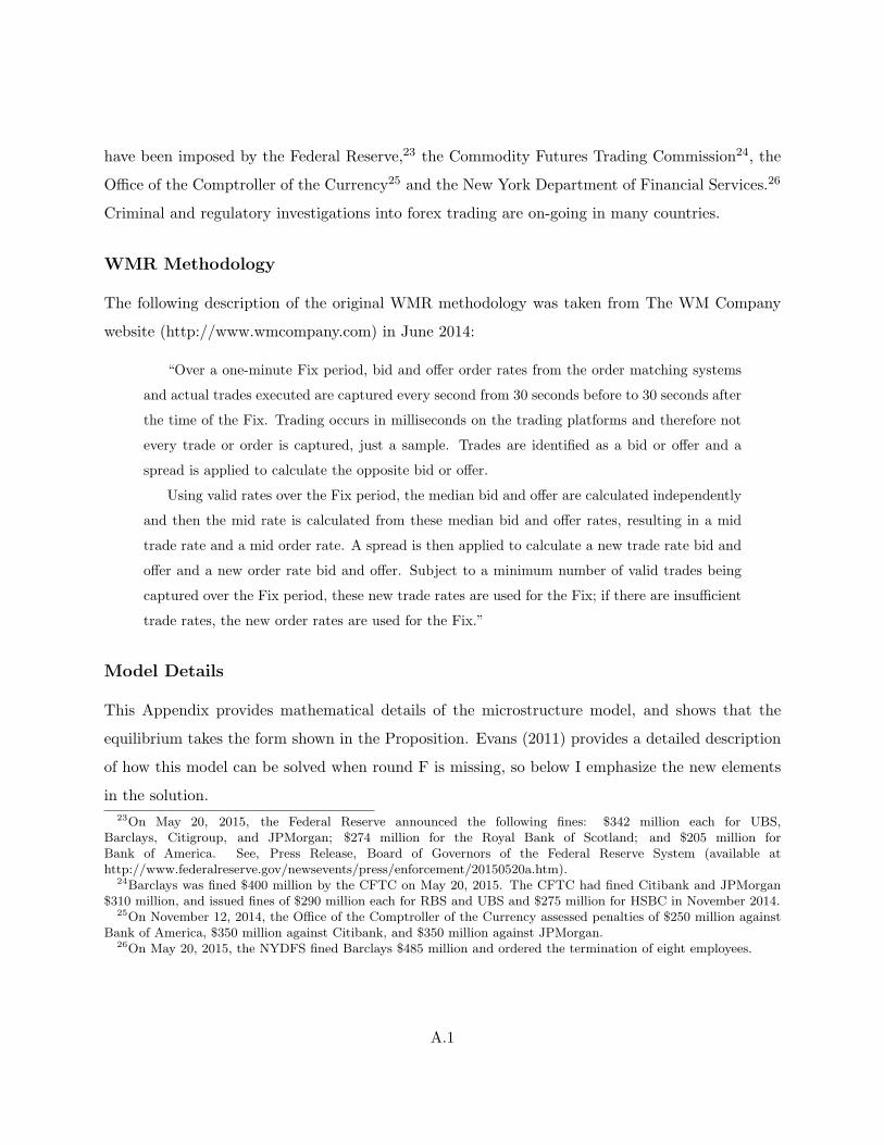
have been imposed by the Federal Reserve,23 the Commodity Futures Trading Commission24, the
Office of the Comptroller of the Currency25 and the New York Department of Financial Services.26
Criminal and regulatory investigations into forex trading are on-going in many countries.
WMR Methodology
The following description of the original WMR methodology was taken from The WM Company
website (http://www.wmcompany.com) in June 2014:
“Over a one-minute Fix period, bid and offer order rates from the order matching systems
and actual trades executed are captured every second from 30 seconds before to 30 seconds after
the time of the Fix. Trading occurs in milliseconds on the trading platforms and therefore not
every trade or order is captured, just a sample. Trades are identified as a bid or offer and a
spread is applied to calculate the opposite bid or offer.
Using valid rates over the Fix period, the median bid and offer are calculated independently
and then the mid rate is calculated from these median bid and offer rates, resulting in a mid
trade rate and a mid order rate. A spread is then applied to calculate a new trade rate bid and
offer and a new order rate bid and offer. Subject to a minimum number of valid trades being
captured over the Fix period, these new trade rates are used for the Fix; if there are insufficient
trade rates, the new order rates are used for the Fix.”
Model Details
This Appendix provides mathematical details of the microstructure model, and shows that the
equilibrium takes the form shown in the Proposition. Evans (2011) provides a detailed description
of how this model can be solved when round F is missing, so below I emphasize the new elements
in the solution.
23On May 20, 2015, the Federal Reserve announced the following fines: $342 million each for UBS,Barclays, Citigroup, and JPMorgan; $274 million for the Royal Bank of Scotland; and $205 million forBank of America. See, Press Release, Board of Governors of the Federal Reserve System (available athttp://www.federalreserve.gov/newsevents/press/enforcement/20150520a.htm).
24Barclays was fined $400 million by the CFTC on May 20, 2015. The CFTC had fined Citibank and JPMorgan$310 million, and issued fines of $290 million each for RBS and UBS and $275 million for HSBC in November 2014.
25On November 12, 2014, the Office of the Comptroller of the Currency assessed penalties of $250 million againstBank of America, $350 million against Citibank, and $350 million against JPMorgan.
26On May 20, 2015, the NYDFS fined Barclays $485 million and ordered the termination of eight employees.
A.1

Market Participants
Investors The forex orders from investor n during day t are determined by their desire to maxi-
mize expected utility defined over wealth on day t+ 1 :
U in,t = E
−θ exp(−θW in,t+1)|Ω
in,t
, (9)
with θ > 0 where W in,t+1 is the wealth of investor n at the start of round i on day t + 1. The
information available to investor n at the start of round i on day t is denoted by Ωin,t.
At the start of day t, investors receive two pieces of information. First, everyone learns the
dividend paid by each unit of forex, Dt. Second, each investor n receives foreign income Yn,t,
that comprises an aggregate component, Yt, and an idiosyncratic component ξn,t. The value of Yn,t
represents private information to each investor, but they do not initially observe either component.
In equilibrium each investor learns the value of Yt by the end of day t. In the interim, the conditional
distribution of Yt is given by Yt|Yn,t ∼ N(κnYn,t, (1− κn)σ2y), where κn ≡ σ2
y/(σ2y + σ2
ξ ).
Investors face makes three decisions each day. In rounds i and iii they choose their trades with
dealers, while in round ii they choose their Fix order which is filled in round f. Let Ain,t denote
investor n’s holding of forex at the end of round i. Since dealers quote common prices in equilibrium
(i.e. Sid,t = Si
t), the budget constraints facing the investor are
W iiin,t = Ai
n,t(Siiit − Si
t) + (Afn,t −Ai
n,t)(Siiit − Sf
t ) +W in,t + Si
tYn,t, and (10a)
W in,t+1 = Aiii
n,t(Sit+1 +Dt+1 − (1 + r)Siii
t ) + (1 + r)W iiin,t. (10b)
In round I, Ain,t is chosen to maximize UI
n,t subject to (10) with private information Ωin,t =
n
Sid,t
dd=1, Yn,t, Dt,Ω
iiin,t1
o
. The forex orders of investor n are Ain,t − Aiii
n,t1 − Yn,t. In round
ii, the investor chooses Afn,t to maximize UII
n,t subject to (10) with private information Ωiin,t =
n
Siid,t
dd=1,Ω
in,t
o
. The investors’ Fix order is Afn,t −Ai
n,t. In round iii the investor chooses Aiiin,t to
maximize UIIIn,t subject to (10b) with Ω
iiin,t =
n
Siiid,t
dd=1, S
ft ,Ω
iin,t
o
. Their round iii forex orders are
Aiiin,t −Af
n,t.
A.2

Dealers Each dealer d makes decisions during day t to maximize expected utility
U id,t = E
−θ exp(−θW id,t+1)|Ω
id,t
,
where W id,t and Ω
id,t denote the wealth and information of dealer d at the start of round i on day
t. The problem for each dealer is to choose the price quotes Sid,t in rounds i = i,ii,f,iii and
inter-dealer trades, T id,t, in rounds ii, f and iii to maximize expected utility given the following
sequence of budget constraints:
W iid,t = W i
d,t + (Aid,t − Z i
d,t)(Siit − Si
t) + Z id,t(S
id,t − Si
t), (11a)
W fd,t = W ii
d,t + (Aiid,t + T ii
d,t − Z iid,t)(S
ft − Sii
t ) + Z iid,t(S
iid,t − Sii
t ), (11b)
W iiid,t = W f
d,t + (Afd,t + T f
d,t − Zfd,t − Fd,t)(S
iiit − Sf
t ) (11c)
W id,t+1 = (1 + r)W iii
d,t + (Aiiid,t + T iii
d,t − Z iiid,t)(S
it+1 +Dt+1 − (1 + r)Siii
t )
+Z iiid,t(S
iiid,t − Siii
t ). (11d)
whereAid,tdenotes the dealer’s forex holding at the start of round i.
Dealers choose their quotes in each round, and their trades in rounds ii, f and iii to max-
imize expected utility U id,t subject to the budget constraints in (11) with their available infor-
mation. The information available to dealer d at the start of round i is Ωid,t = Dt,Ω
iiid,t1.
At the start of round ii the dealer knows his Fix orders as well as the quotes and his trades
from round i: Ωiid,t =
n
Sid,t
dd=1, Z
id,t, Fd,t,Ω
id,t
o
. Importantly individual dealers do not know
aggregate imbalance in trades from round i or the aggregate imbalance in Fix orders. By the
start of the Fix round individual dealers have seen round ii quotes and aggregate order flow, so
Ωfd,t =
n
X iit , S
iid,t
dd=1, S
iib,t, Z
iid,t,Ω
iid,t
o
. Finally, at the start of round III individual dealers know
the Fix benchmark and the aggregate order from round f, so Ωiiid,t =
n
Xft , S
fd,t
dd=1, Z
fd,t,Ω
fd,t
o
.
A.3

The Broker The foreign exchange broker chooses quotes in rounds ii, f and iii, Siib,t S
fb,t and Siii
b,t,
to maximize expected utility defined over wealth on day t + 1: U ib,t = E[ − θ exp(−θW i
b,t+1)|Ωib,t],
where W ib,t and Ω
ib,t denote the wealth and information of the broker at the start of round i on
day t. The broker’s wealth follows the dynamics of dealer d0s wealth in (11) except that Z id,t = 0,
Fd,t = 0 and T iid,t = T f
d,t = T iiid,t = 0 because brokers do not receive customer orders in round i, Fix
orders, nor can they initiate trades in rounds ii, f and iii. The information available to brokers
evolves in the same way as that of dealer d with Z id,t = 0 and Fd,t = 0
Solving for the Equilibrium
The steps here closely follow those on pages 279-287 in Evans (2011), so I concentrate on the new
elements arising from the introduction of the Fix.
An equilibrium in this model comprises: (i) investors’ trades in rounds i and iii, and their Fix
orders in round ii; (ii) the forex price quotes by dealers and the broker; and (iii) dealers’ trading
decisions in rounds ii, f and iii. All these decisions must be optimal in the sense that they maximize
the expected utility of the respective agent given available information and they must be consistent
with market clearing conditions:
dX
d=1
Z id,t =
Z 1
0(Ai
n,t −Aiiin,t1 − Yn,t)dn. (12a)
dX
d=1
Zjd,t + Z j
b,t =
dX
d=1
T jd,t for j = ii,f (12b)
dX
d=1
Z iiid,t =
Z 1
0(Aiii
n,t −Afn,t)dn, and Z iii
b,t =dX
d=1
T iiid,t. (12c)
Condition (12a) states that in aggregate incoming forex orders received by dealers in round i
equal investors desired change in forex holdings: Ain,t − Aiii
n,t1 − Yn,t. Market clearing in rounds
ii and f requires that aggregate incoming orders received by dealers and the broker equal the
aggregate forex purchases initiated by dealers as shown in (12b). In round iii condition (12c)
shows that dealers’ incoming orders must match investors desired change in forex holdings, and the
broker’s order must match dealer-initiated trades. The market clearing condition for Fix orders
A.4

was given in equation (1).
Information Consider the common information of dealers at the start of round i: Ωid,t =
T
dΩid,t.
In round i common information is Ωid,t =
Dt,Ωiiid,t1
. Trading between dealers and investors in
round i does not change dealer’ common information so Ωiid,t = Ω
id,t.
Next we turn to the common information revealed by trading in rounds ii and f. Equations (3)
and (4a) imply that aggregate order flows in rounds ii and f are
X iit =
dX
d=1
αiizZ
id,t + αii
aAt1 = αiizβYt + αii
aAt1, (13)
Xft =
dX
d=1
αfzZ
id,t +
dX
d=1
αffFd,t + αf
aAt1 + αfxX
iit = αf
fβYt + αffFt + αf
aAt1 + αfxX
iit , (14)
In equilibrium (shown below), Ft = Ht and At = At1 + Yt −Ht. Following the steps on page 279
we can use this expression with the equations above to show that order flow from round ii reveals
the value of Yt, so Ωfd,t =
Yt,Ωiid,t
, and order flow from round f reveals Ht, so Ωiiid,t =
Ht,Ωfd,t
.
From these results it follows that (i) E[Yt|Ωid,t] = 0, (ii) E[Ht|Ω
iid,t] = 0, and (iii) E[At1|Ω
id,t] = At1
because At1 =P1
i=i(Yti−Hti) and Yti−Hti ∈ Ωid,t for i ≥ 1. Consequently, X ii
t −E[X iit |Ω
iid,t] =
αiizβYt and Xf
t − E[Xft |Ω
fd,t] = αf
fHt. We can therefore rewrite (2b) and (2c) as
Sft = Sii
t + λiiaAt1 + λii
xαiizβYt, (15a)
Siiit = Sf
t + λfaAt1 + λf
xαffHt, (15b)
Now consider the common information of investors, Ωit =
T
nΩin,t. In round i all investors
observe the dividend shock from which they compute the value for Dt. They also observe the
common equilibrium quote from all the dealers, so Ωit =
Sit, Dt,Ω
iiit1
. Equation (15) implies that
all investors know the values of Yt and Ht by the end of each days so At1 ∈ Ωit1. It therefore
follows from (15) that Ωiiit =
Yt, Ht,Ωit1
. In sum, therefore, dealers and investors share the
same common information set in rounds i and iii:
Ωid,t = Ω
it =
Dt,Ωiiit1
and Ωiiid,t = Ω
iiit = Yt, Ht,Ω
it .
A.5

Investors Trades Consider investor n0s choice of FX holdings in round iii, Aiiin,t. As in the PS
model, in equilibrium the distribution of excess returns Rt+1 ≡ Sit+1 +Dt+1 − (1 + r)Siii
t is normal
conditioned on information, Ωiiin,t. Maximizing expected utility U iii
n,t subject to (10b) gives
Aiiin,t =
1γE[Si
t+1 +Dt+1 − (1 + r)Siiit |Ωiii
n,t], (16)
where γ ≡ θV[Rt+1|Ωiiin,t]. In equilibrium, all investors have the same conditional expectations
concerning Sit+1 and Dt+1, so their overnight FX holdings are the same, i.e., Aiii
n,t = Aiiit for all
n ∈ [0, 1].
In round i, investor n chooses Ain,t to maximize U i
n,t subject to the sequence of budget constraints
in (10). In equilibrium, these constraints take the same form as in the PS model (see below) so,
like there, optimal round i holdings are given by
Ain,t = ηiaA
iiit1 + ηisE[S
iiit − Si
t|Ωin,t]. (17)
(The coefficients ηia and ηis are given by the formulae on pages 299 and 230 in Evans (2011) with
Yt −Ht replacing Yt.) From (15) and (2b) we find that
E[Siiit − Si
t|Ωin,t] = (λii
a + λfa)At1 + λii
xαiizβE[Yt|Ω
in,t] + λf
xαffE[Ht|Ω
in,t].
= (λiia + λf
a)At1 + λiixα
iizβκnYn,t
so
Ain,t = ηisλ
iixα
iizβκnYn,t + (ηis(λ
iia + λf
a) + ηia)Aiiit1 = ηisλ
iixα
iizβκnYn,t +Aiii
t1.
because λiia + λf
a = (1 − ηia)/ηis (see below). By definition, the FX order from investor n in round
i is Ain,t − Aiii
n,t1 − Yn,t = (ηisλiixα
iizβκn − 1)Yn,t. Since all dealers quote a common round i price in
equilibrium, each dealer receives an equal share of investors’ FX orders, Z id,t = (β/d)Yt + εd,t with
β = 1/(ηisλiixα
iizκn − 1), as shown in (4a).
At the start of round ii investors optimally choose their Fix orders, Afn,t − Ai
n,t to maximize
U iin,t subject to the sequence of budget constraints in (10). Once again we can follow Evans (2011)
A.6

to show that the optimal choice is
Afn,t −Ai
n,t = ηfaAiiin,t1 + ηfsE[S
iiit − Sf
t |Ωiin,t]. (18)
Substituting for Siiit − Sf
t from (15) gives E[Siiit − Sf
t |Ωiin,t] = λf
aAt1, so traders’ Fix orders are
Afn,t − Ai
n,t = (ηfa + ηfsλfa)At1. We will see below that when dealers quote prices in round f
to efficiently share risk, ηfa + ηfsλfa = 0. Consequently, Af
n,t = Ain,t, so traders find it optimal
not to submit Fix orders in equilibrium and Ft =R
n
Afn,t −Ai
n,t
dn + Ht = Ht (noted above).
Furthermore, when Afn,t = Ai
n,t the budget constraints in (10b) simplify to those in the PS model,
which is why (16) and (17) take the same form.
Quotes As in the PS model, dealers and the broker quote prices to support an efficient risk-
sharing allocation of forex holdings. This means that the round iii quote is chosen so that investors
are willing to hold the entire stock of forex, At. Recall that the distribution of Rt+1 conditioned
on individual investors information, Ωiiin,t, is the same across all investors, and is equal to the
distribution conditioned on common information, Ωiiit . Under these circumstances, (16) implies
that the aggregate demand for forex is At = 1γE[Rt+1|Ω
iiit ]. Combining this expression with the
definition of Rt+1 gives,
Siiit = 1
1+rE
Siiit+1 +Dt+1|Ω
iiit
− 11+r
E
Siiit+1 − Si
t+1|Ωiiit
− γ(1+r)At.
Equation (2) of Proposition 1 implies that E[Siiit+1 − Si
t+1|Ωiiit ] = (λii
a + λfa)At. Making this substi-
tution in the expression above and solving forward gives
Siiit =
1X
i=1
11+r
i
E [Dt+i − (γ + λiia + λf
a)At+i1|Ωiiit ] . (19)
This equation identifies the value for the round iii quote needed to induce investors to hold At
given their expectations concerning future dividends and holdings, Dt+1+i, and At+i.
Efficient risk-sharing and market clearing imply that the aggregate investor demand for forex,
At, be equal to aggregate holdings at the end of day t−1, At1, plus foreign income received during
round i, Yt =R 10 Yn,tdn, minus the the forex needed to fill the hedger Fix orders, Ht. Hence, the
A.7

equilibrium dynamics of investors forex holdings follow At = At1+Yt−Ht (as noted above). Using
this equation to forecast investor demand, and the facts that E[Dt+i|Ωiiit ] = Dt, E[Yt+i|Ω
iiit ] = 0
and E[Ht+i|Ωiiit ] = 0 for all i > 0, we can rewrite (19) as
Siiit = 1
rDt − 1
r(γ + λii
a + λfa)At. (20)
We have thus found the value of the round iii quote that achieves an efficient risk-sharing allocation.
Dealers’ quotes in round i and ii are determined in exactly the same way as in the PS model.
Dealers choose Sit such that the allocation of holdings is ex ante efficient conditioned on common
information Ωid,t, i.e. E[Z i
d,t|Ωid,t] = 0. To find this value for Si
t, we take expectations with respect
to dealers’ common information on both sides of the market clearing condition in (12a):
dX
d=1
E[Z id,t|Ω
id,t] =
Z 1
0E[Ai
n,t −Aiiin,t1 − Yn,t|Ω
id,t]dn.
Substituting for Ain,t with (17) and noting that E[Yn,t|Ω
id,t] = 0 for all n gives
dX
d=1
E[Z id,t|Ω
id,t] = ηisE[S
iiit − Si
t|Ωidt] + (ηia − 1)Aiii
t1.
Finally, we impose the risk-sharing restriction E[Z id,t|Ω
id,t] = 0, and solve for Si
t as
Sit = E[Siii
t |Ωid,t]− (λii
a + λfa)At1. (21)
where λiia + λf
a ≡ (1− ηia)/ηis.
In rounds ii and f dealers choose Siit and Sf
t so that E[Fd,t|Ωiid,t] = 0 and E[Fd,t|Ω
fd,t] = 0.
In words, dealers choose quotes so there is no expected imbalance in Fix orders conditioned on
common dealer information. Recall that Fix orders comprise orders from hedgers and investors,
Ft = Ht+R
n
Afn,t −Ai
n,t
dn. Since E[Ht|Ωiid,t] = 0, dealers will achieve an ex ante efficient allocation
with their choice for Siit provided E[Af
n,t−Ain,t|Ω
iid,t] = 0. We showed above that the optimal choice
for Afn,t −Ai
n,t depends on At1 and E[Siiit − Sf
t |Ωiin,t]. Neither of these terms depends on the value
of Siit . Dealers can therefore set
Siit = Si
t (22)
A.8

to eliminate the risk of unexpected round i trades (just as in the PS model) and use their choice
for Sft to ensure that E[Fd,t|Ω
iid,t] = 0 and E[Fd,t|Ω
fd,t] = 0. This is achieved by setting
Sft = Si
t + λiiaAt1 + λii
xαiizβYt, (23)
with λiia = (1 − ηia)/η
is − (ηfa/η
fs ) and λii
x = −1r(γ + λii
a + λfa)/α
iizβ. (Recall that both At1 and Yt
are in Ωfd,t) This choice for Sf
t implies that Siiit − Sf
t = 1r(γ + +λii
a + λfa)Ht + λf
aAt1, so traders’
optimal fix orders are
Afn,t −Ai
n,t = ηfaAiiin,t1 + ηfsE[S
iiit − Sf
t |Ωiin,t] = (ηfa + ηfsλ
fa)At1 = 0.
This means that Ft = Ht +R
n
Afn,t −Ai
n,t
dn = Ht, so E[Fd,t|Ωfd,t] =
1DE[Ht|Ω
fd,t] +E[ξt|Ω
fd,t] = 0
and E[Fd,t|Ωiid,t] = 0 (by iterated expectations) as required. Finally, it is straightforward to check
that (20) - (23) can be rewritten in the form of (2) with λx = −(γ + λiia + λf
a)/(βrαz) and λfx =
1αffr(γ + λii
a + λfa).
Dealer Trades All that now remains is to confirm that inter-dealer trades take the form of (3).
Dealers trades in round iii take the same form as in the PS model and allow each dealer to eliminate
their overnight FX holdings. Hence, in equilibrium, the budget constraints in (11b) and (11d) of
dealer d become
W id,t+1 = (1 + r)[W f
d,t + Afd,t(S
iiit − Sf
t )− (Zfd,t − E[Zf
d,t|Ωfd,t])(S
iiit − Sf
t )], (24)
where Afd,t ≡ Af
d,t + T fd,t − E[Zf
d,t|Ωfd,t] − Fd,t is dealer’s desired FX position. In round f dealers
choose T fd,t given the incoming orders from other dealers following BNE strategies, Zf
d,t, and the fix
orders he took at the start of round ii, Fd,t, such that Afd,t maximizes expected utility given (24).27
As in the PS model, the dealer’s desired position is given by
Afd,t =
11+dϕ
faAt1 +
11+dϕ
fyE[Ft|Ω
iid,t], (25)
27Notice that dealer d cannot condition his choice for T fd,t on actual incoming orders, Zf
d,t, because all dealersmust act simultaneously. Instead, each dealer must choose T f
d,t based on his expectations regarding incoming ordersE[Zf
d,t|Ωiid,t].
A.9

where ϕfy and ϕf
a are coefficients again given in the appendix of Evans (2011). We showed above
that Siiit −Sf
t = λfaAt1+λf
xαffHt, (with Ht = Ft) so dealer’s use their private forecast of aggregate
imbalance in Fix orders to determine their desired position. Dealers’ trades in round ii are derived
from their desired position in an analogous fashion:
Aiid,t =
11+dϕ
iiaAt1 +
11+dϕ
iiyE[Yt|Ω
iid,t], (26)
because Sft − Sii
t = λiiaAt1 + λii
xαiizβYt. Dealers’ desired position in round ii depend on the private
forecasts of aggregate income. As in the PS model, I assume that dealers view the shocks that
distribute traders orders in round i and Fix orders in round ii as i.i.d. normal variables so their
private forecasts are given by E[Yt|Ωiid,t] = κdZd,t and E[Ft|Ω
iid,t] = κfFd,t. (Recall from (4a) that
Zd,t is a noisy signal of aggregate income.)
We can now compute the BNE trading strategies for each dealer in rounds ii and f. If all other
dealers trade according to (3), and orders are equally split between the broker and the dealers
because they quote the same price, incoming order flow from other dealers is
Z iid,t =
11+dα
iizβYt +
11+dα
iiaαaAt1.
Dealer d0s forecast of this order flow is therefore
E[Z iid,t|Ω
iid,t] =
11+dα
iizβE[Yt|Ω
iid,t] +
11+dα
iiaAt1.
By definition, dealer d0s trade is given by T iid,t = Aii
d,t − Aiid,t + E[Z ii
d,t|Ωiid,t]. Since dealers hold no
overnight positions, their FX holdings at the start of round ii simply reflect the customer orders
they filled in round i, i.e., Aiid,t = −Z i
d,t. Combining this fact with the definition above gives
T iid,t = Aii
d,t + Z id,t + E[Z ii
d,t|Ωiid,t],
= 11+d (ϕii
y + αiizβ)E[Yt|Ω
iid,t] + Z i
d,t +1
1+d (ϕiia + αii
a)At1,
=
1 + 11+d (ϕii
y + αiizβ)κd
Z id,t +
11+d (ϕii
a + αiia)At1. (27)
Thus, the BNE strategy for each dealer is to initiate an inter-dealer trade that is a linear function
A.10

of his own customer orders, Z id,t, and the outstanding stock of FX, At1, as shown in equation (3a)
of the Proposition. Equating coefficients gives the formulas for the αii coefficients.
In the Fix round incoming orders are
Zfd,t = 1
1+dαfzβY t +
11+dα
faAt1 +
11+dα
ffFt +
11+dα
fxX
iit .
= 11+d(α
fz + αf
xαiiz )βY t +
11+d(α
fa + αf
xαiia)At1 +
11+dα
ffFt
so
E[Zfd,t|Ω
fd,t] = 1
1+d(αfz + αf
xαiiz )βE[Yt|Ω
iid,t] +
11+d(α
fa + αf
xαiia)At1+
11+dα
ffE[Ft|Ω
fd,t].
Substituting these terms in the definition, Afd,t − Af
d,t = Afd,t − Aii
d,t + (Z iid,t − E[Z ii
d,t|Ωiid,t]), and
simplifying with (26) and (25) gives
Afd,t −Af
d,t =1
1+d (ϕfa − ϕii
a)At1 +1
1+dϕfyκfFn,t − 1
1+dϕiiyκdZd,t +
11+dα
iizβ(Yt − κdZd,t).
Finally, by definition T fd,t = Af
d,t−Afd,t+E[Zf
d,t|Ωfd,t]+Fd,t. So substituting from above we find that
T fd,t = 1
1+d (ϕfa − ϕii
a)At1 +1
1+dϕfyκfFn,t − 1
1+dϕiiyκdZd,t +
11+dα
iizβ(Yt − κdZd,t)
+ 11+dα
ffκfFd,t +
11+d(α
fa + αf
xαiia)At1 +
11+d(α
fz + αf
xαiiz )βκdZd,t + Fd,t
= 11+d (ϕf
a − ϕiia + αf
a + αfxα
iia)At1 +
11+d (ϕf
yκf + αffκf + 1)Fd,t
+ 11+d(X
iit − αii
aAt1) +1
1+d((αfz + αf
xαiiz − αii
z )β − ϕiiy)κdZd,t
= (αfa/d)At1 + αf
fFd,t + (αfx/d)X
iit + αf
zZd,t
as shown in the Proposition. Equating coefficients gives the formulas for the αf coefficients.28
28Clearly, this sequencing of events is much simpler than the continuous process of price-quotes and trades thattakes place during the actual Fix window. To check the robustness of the equilibrium to this simple structure, I alsoconsidered a version of the model where the Fix benchmark was determined by the average of the round f and iiiprices. In this equilibrium Xf
t affects the determination of the benchmark price, but other features of the equilibriumare unchanged.
A.11

Additional Empirical Analysis
Data
Table A.1 provides information on the Gain Capital used in the empirical analysis. The rates are
listed in column (i). Columns (ii) and (iii) report the span and scope of the tick-by-tick data for
each rate. For 11 currency pairs, I use a decade of tick-by-tick bid and offer rates starting at
midnight on December 31 st. 2003. Continuous data is not available for the other currency pairs
in 2004 – 2007 so I use tick-by-tick rates starting after midnight on December 31 st. 2007, when
continuous data becomes available. The data samples for all the currency pairs end at midnight
on December 31 st. 2013. As column (iii) shows, the time series for each currency pair contains
tens of millions of data points. Each series contains a date and time stamp, where time is recorded
to the nearest 1/100 of a second, and a bid and offer rate. Unlike standard time series, the time
between observations is irregular, ranging from a few minutes to a hundredth of a second.
As noted in the text, I checked the accuracy of the Gain data by comparing the mid-points from
the tick-by-tick data with the 4:00 pm Fix benchmarks on each trading day in the sample. Fixes
are computed as the mid point of the median bid and ask rates across multiple transactions in a one
minute window that starts 30 seconds before 4:00 pm. For comparison, I computed an analogous
mid-point from the median of the bid and ask rate data on every trading day covered by each
currency pair. Differences between this mid-point and the Fixes represent the tracking error of the
Gain data relative to the rates used to determine the Fixes. Table A.1 reports the percentiles of the
tracking-error distribution, measured in basis points relative to the Fix benchmark, for each of the
currency pairs I study. I separate the tracking errors on end-of-month trading days from the errors
on other trading days and report percentiles for both the intra- and end-of-month distributions.
Bootstrap Distribution
I summarize the behavior of forex prices away from the Fix with a bootstrap distribution of price
changes computed from 10,000 randomly chosen times (excluding the times of scheduled releases
U.S. macro data, the 4:00 WMR Fix and ECB Fix). Table A.2 reports statistics for this distribution
of spot rate changes over horizons of five, fifteen, and thirty minutes. Columns (iii) - (vii) report
statistics for the distribution of changes in the log rates expressed in basis points per minute, i.e.,
A.12
Table A.1: Data Characteristics
Intra Month Trading Days End-of-Month Trading Days
FX Rate Data Span Prices Number Tracking Error Distribution Number Tracking Error DistributionPercentiles (basis points) Percentiles (basis points)
(millions) 5% 50% 95% 5% 50% 95%
(i) (ii) (iii) (iv) (v) (vi) (vii) (viii) (ix) (x) (xi)
A: EUR/USD 2004-13 55.370 2420 -1.113 0.055 1.209 117 -1.232 0.109 1.771CHF/USD 2004-13 51.966 2258 -1.510 0.060 1.761 106 -2.462 0.058 2.345JPY/USD 2004-13 38.931 2204 -1.268 0.140 1.790 104 -3.241 0.207 2.608USD/GBP 2004-13 60.859 2421 -1.087 0.083 1.200 116 -1.258 0.051 2.566
B: CHF/EUR 2004-13 37.858 2373 -1.144 0.000 1.145 116 -2.135 0.000 1.243JPY/EUR 2004-13 78.813 2421 -1.538 0.021 1.542 117 -4.939 0.090 2.822NOK/EUR 2008-13 15.780 1291 -1.710 0.008 2.015 62 -2.624 0.252 3.829NZD/EUR 2008-13 56.633 1414 -2.211 0.079 2.381 68 -2.927 0.284 3.844SEK/EUR 2008-13 17.424 1288 -1.643 -0.010 1.551 59 -2.336 -0.089 1.980
C: AUS/GBP 2008-13 68.169 1476 -1.209 0.225 1.730 69 -2.695 0.544 4.016CAD/GBP 2008-13 57.455 1478 -1.180 0.293 1.777 71 -1.676 0.371 2.578CHF/GBP 2004-13 83.686 2417 -1.476 0.087 1.634 116 -3.412 0.020 2.013EUR/GBP 2004-13 41.643 2339 -1.651 0.114 2.176 115 -2.302 0.157 2.523JPY/GBP 2004-13 88.578 2418 -1.564 0.020 1.582 116 -2.612 0.137 2.378NZD/GBP 2008-13 58.216 1409 -2.197 0.089 2.350 67 -2.529 0.397 5.046
D: AUS/USD 2004-13 49.016 2398 -1.601 0.144 2.283 116 -2.373 -0.117 2.053CAD/USD 2004-13 36.163 2404 -1.461 0.138 1.864 116 -1.909 0.256 2.821DKK/USD 2008-13 66.719 1305 -0.696 0.081 0.825 59 -0.779 0.115 0.996NOK/USD 2008-13 55.350 1306 -1.696 0.071 2.152 62 -3.983 0.602 3.999SEK/USD 2008-13 58.296 1297 -1.811 0.053 1.792 59 -2.783 0.101 2.067SGD/USD 2008-13 10.567 1200 -1.440 0.000 1.517 61 -1.980 0.168 1.982
Notes: Columns (i) - (iii) show the data span and the number of quotes (in millions) for each of the currency pairs in the data set. Columns (iv) and
(viii) report the number of intra-month and end-of-month trading days for which there are intraday quotes, respectively. Quote errors on each day
are defined as the difference between the mid-point of the average bid and ask quotes computed over a one minute window centered on 4:00 pm and
the Fix benchmark. Quote errors are expressed in basis points. Columns (v) - (vii) and (ix) - (xi) show the 5th., 50th. and 95th. percentiles of the
quote error distribution computed on all intra-month and end-of-month trading days.
A.13
∆hst ≡ (ln(St+h)−ln(St))∗10000/h for horizons h = 5, 15, 60 minutes, where St denotes the mid-
point rate a time t. Columns (viii) and (ix) report the first-order autocorrelation in ∆hst+h and the
p-value for the null of a zero autocorrelation, respectively. Column (x) reports the Kolmogorov-
Smirnov (KS) test for the null that the two conditional distributions f(∆hst+h|∆hst > 0) and
f(∆hst+h|∆hst ≤ 0) are the same. The p-value for the test is shown in column (xi).
As Table A.2 shows, the rate-change distributions have several common characteristics across
all the currency pairs. First, the dispersion in the rate-change distributions declines as the horizon
rises. Columns (iii) and (iv) show that the absolute values for the 5th. and 95th. percentiles of
the distributions fall as the horizon rise from five to 30 minutes. The change in dispersion is also
reflected by the standard deviations shown in column (v), which fall as the horizon rises. Second, all
the rate-change distributions are strongly leptokurtic. As column (vii) shows, the kurtosis statistics
across all the currency pairs are large; much larger than the value of three implied by the normal
distribution. These statistics indicate that atypically large changes in rates occur quite frequently
away from the Fixes and scheduled macro news releases.
The third feature concerns temporal dependence between rate changes. Column (viii) shows
that rate changes display some small degree of autocorrelation. Across currency pairs, the autocor-
relation is generally negative.29 This fact accounts for the declining dispersion of the rate-change
distributions as the horizon rises, noted above. Although small in (absolute) value, the statistics in
column (ix) indicate that many of the estimated autocorrelation coefficients are statistical signifi-
cant at standard levels. There is also evidence of temporal dependence from the KS tests reported
in column (ix). Under the null of temporal independence, future changes in rates should not de-
pend on the sign of past changes, i.e., f(∆hst+h|∆hst > 0) = f(∆hst+h|∆
hst ≤ 0). As column (x)
shows, this null can easily be rejected at standard levels of significance for most currency pairs and
horizons h.
29While the estimated autocorrelations imply that future rate changes are forecastable using past rates, thesecorrelations are computed from the mid-points of the bid and ask rates. As such, the estimated autocorrelationsare not a reflection of so-called bid-ask bounce. Nor do they imply that the future returns available to traders (i.e.changes in log rates that account for the bid/offer spread) can be forecast.
A.14
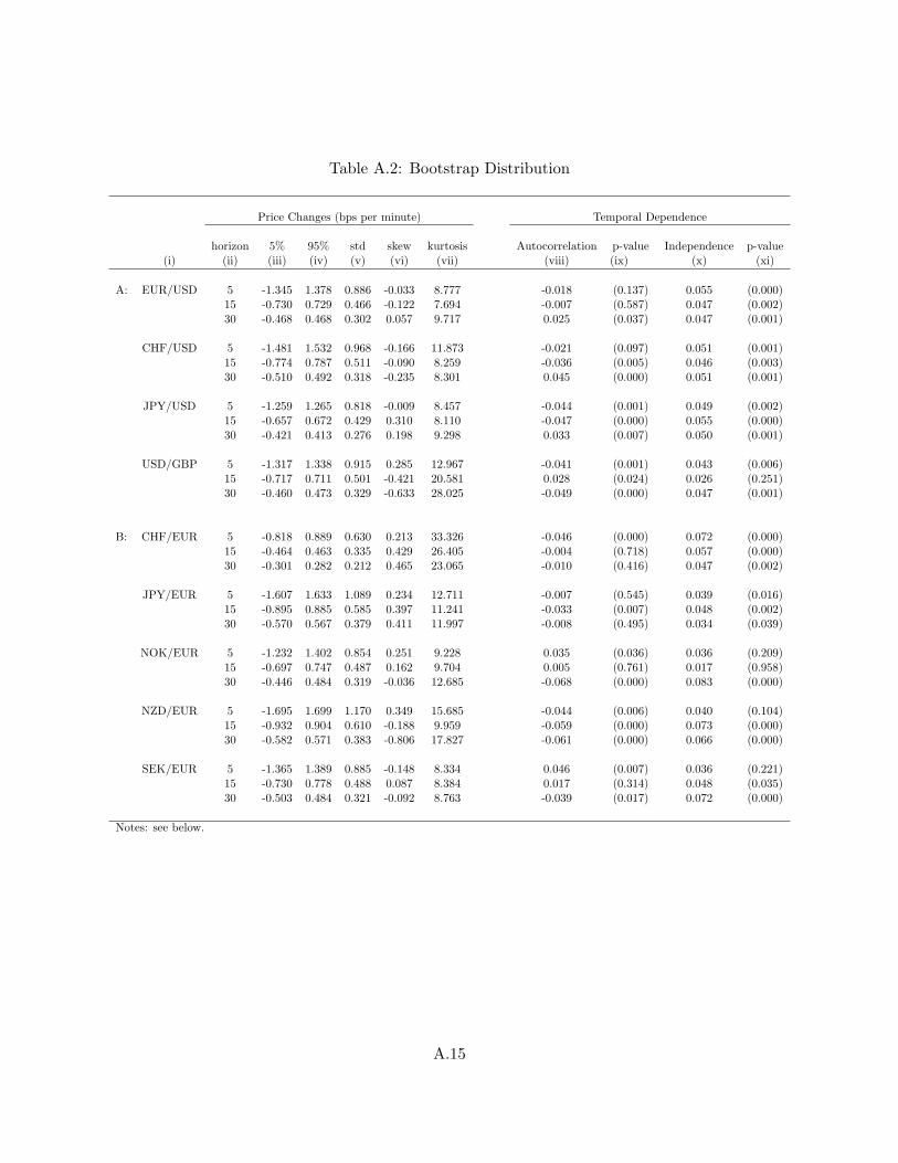
Table A.2: Bootstrap Distribution
Price Changes (bps per minute) Temporal Dependence
horizon 5% 95% std skew kurtosis Autocorrelation p-value Independence p-value(i) (ii) (iii) (iv) (v) (vi) (vii) (viii) (ix) (x) (xi)
A: EUR/USD 5 -1.345 1.378 0.886 -0.033 8.777 -0.018 (0.137) 0.055 (0.000)15 -0.730 0.729 0.466 -0.122 7.694 -0.007 (0.587) 0.047 (0.002)30 -0.468 0.468 0.302 0.057 9.717 0.025 (0.037) 0.047 (0.001)
CHF/USD 5 -1.481 1.532 0.968 -0.166 11.873 -0.021 (0.097) 0.051 (0.001)15 -0.774 0.787 0.511 -0.090 8.259 -0.036 (0.005) 0.046 (0.003)30 -0.510 0.492 0.318 -0.235 8.301 0.045 (0.000) 0.051 (0.001)
JPY/USD 5 -1.259 1.265 0.818 -0.009 8.457 -0.044 (0.001) 0.049 (0.002)15 -0.657 0.672 0.429 0.310 8.110 -0.047 (0.000) 0.055 (0.000)30 -0.421 0.413 0.276 0.198 9.298 0.033 (0.007) 0.050 (0.001)
USD/GBP 5 -1.317 1.338 0.915 0.285 12.967 -0.041 (0.001) 0.043 (0.006)15 -0.717 0.711 0.501 -0.421 20.581 0.028 (0.024) 0.026 (0.251)30 -0.460 0.473 0.329 -0.633 28.025 -0.049 (0.000) 0.047 (0.001)
B: CHF/EUR 5 -0.818 0.889 0.630 0.213 33.326 -0.046 (0.000) 0.072 (0.000)15 -0.464 0.463 0.335 0.429 26.405 -0.004 (0.718) 0.057 (0.000)30 -0.301 0.282 0.212 0.465 23.065 -0.010 (0.416) 0.047 (0.002)
JPY/EUR 5 -1.607 1.633 1.089 0.234 12.711 -0.007 (0.545) 0.039 (0.016)15 -0.895 0.885 0.585 0.397 11.241 -0.033 (0.007) 0.048 (0.002)30 -0.570 0.567 0.379 0.411 11.997 -0.008 (0.495) 0.034 (0.039)
NOK/EUR 5 -1.232 1.402 0.854 0.251 9.228 0.035 (0.036) 0.036 (0.209)15 -0.697 0.747 0.487 0.162 9.704 0.005 (0.761) 0.017 (0.958)30 -0.446 0.484 0.319 -0.036 12.685 -0.068 (0.000) 0.083 (0.000)
NZD/EUR 5 -1.695 1.699 1.170 0.349 15.685 -0.044 (0.006) 0.040 (0.104)15 -0.932 0.904 0.610 -0.188 9.959 -0.059 (0.000) 0.073 (0.000)30 -0.582 0.571 0.383 -0.806 17.827 -0.061 (0.000) 0.066 (0.000)
SEK/EUR 5 -1.365 1.389 0.885 -0.148 8.334 0.046 (0.007) 0.036 (0.221)15 -0.730 0.778 0.488 0.087 8.384 0.017 (0.314) 0.048 (0.035)30 -0.503 0.484 0.321 -0.092 8.763 -0.039 (0.017) 0.072 (0.000)
Notes: see below.
A.15
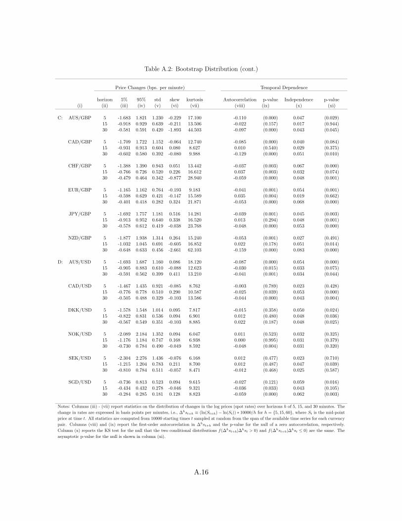
Table A.2: Bootstrap Distribution (cont.)
Price Changes (bps. per minute) Temporal Dependence
horizon 5% 95% std skew kurtosis Autocorrelation p-value Independence p-value(i) (ii) (iii) (iv) (v) (vi) (vii) (viii) (ix) (x) (xi)
C: AUS/GBP 5 -1.683 1.821 1.230 -0.229 17.100 -0.110 (0.000) 0.047 (0.029)15 -0.918 0.929 0.639 -0.211 13.506 -0.022 (0.157) 0.017 (0.944)30 -0.581 0.591 0.420 -1.893 44.503 -0.097 (0.000) 0.043 (0.045)
CAD/GBP 5 -1.709 1.722 1.152 -0.064 12.740 -0.085 (0.000) 0.040 (0.084)15 -0.931 0.913 0.604 0.080 8.627 0.010 (0.540) 0.029 (0.375)30 -0.602 0.580 0.392 -0.080 9.988 -0.129 (0.000) 0.051 (0.010)
CHF/GBP 5 -1.388 1.390 0.943 0.051 13.442 -0.037 (0.003) 0.067 (0.000)15 -0.766 0.726 0.520 0.226 16.612 0.037 (0.003) 0.032 (0.074)30 -0.479 0.464 0.342 -0.877 28.940 -0.059 (0.000) 0.048 (0.001)
EUR/GBP 5 -1.165 1.162 0.764 -0.193 9.183 -0.041 (0.001) 0.054 (0.001)15 -0.598 0.629 0.421 -0.147 15.589 0.035 (0.004) 0.019 (0.662)30 -0.401 0.418 0.282 0.324 21.871 -0.053 (0.000) 0.068 (0.000)
JPY/GBP 5 -1.692 1.757 1.181 0.516 14.281 -0.039 (0.001) 0.045 (0.003)15 -0.913 0.952 0.640 0.338 16.520 0.013 (0.294) 0.048 (0.001)30 -0.578 0.612 0.419 -0.038 23.768 -0.048 (0.000) 0.053 (0.000)
NZD/GBP 5 -1.877 1.938 1.314 0.264 15.240 -0.053 (0.001) 0.027 (0.491)15 -1.032 1.045 0.691 -0.605 16.852 0.022 (0.178) 0.051 (0.014)30 -0.648 0.633 0.456 -2.661 62.103 -0.159 (0.000) 0.083 (0.000)
D: AUS/USD 5 -1.693 1.687 1.160 0.086 18.120 -0.087 (0.000) 0.054 (0.000)15 -0.905 0.883 0.610 -0.088 12.623 -0.030 (0.015) 0.033 (0.075)30 -0.591 0.562 0.399 0.411 13.210 -0.041 (0.001) 0.034 (0.044)
CAD/USD 5 -1.467 1.435 0.921 -0.085 8.762 -0.003 (0.789) 0.023 (0.428)15 -0.776 0.778 0.510 0.290 10.587 -0.025 (0.039) 0.053 (0.000)30 -0.505 0.488 0.329 -0.103 13.586 -0.044 (0.000) 0.043 (0.004)
DKK/USD 5 -1.578 1.548 1.014 0.095 7.817 -0.015 (0.358) 0.050 (0.024)15 -0.822 0.831 0.536 0.094 6.901 0.012 (0.480) 0.048 (0.036)30 -0.567 0.549 0.351 -0.103 8.885 0.022 (0.187) 0.048 (0.025)
NOK/USD 5 -2.089 2.184 1.352 0.094 6.047 0.011 (0.523) 0.032 (0.325)15 -1.176 1.184 0.747 0.168 6.938 0.000 (0.995) 0.031 (0.379)30 -0.730 0.784 0.490 -0.049 8.592 -0.048 (0.004) 0.031 (0.320)
SEK/USD 5 -2.304 2.276 1.436 -0.076 6.168 0.012 (0.477) 0.023 (0.710)15 -1.215 1.204 0.783 0.211 8.700 0.012 (0.487) 0.047 (0.039)30 -0.810 0.784 0.511 -0.057 8.471 -0.012 (0.468) 0.025 (0.587)
SGD/USD 5 -0.736 0.813 0.523 0.094 9.615 -0.027 (0.121) 0.059 (0.016)15 -0.434 0.432 0.278 -0.046 9.321 -0.036 (0.033) 0.043 (0.105)30 -0.284 0.285 0.181 0.128 8.823 -0.059 (0.000) 0.062 (0.003)
Notes: Columns (iii) - (vii) report statistics on the distribution of changes in the log prices (spot rates) over horizons h of 5, 15, and 30 minutes. The
change in rates are expressed in basis points per minutes, i.e., ∆hst+h ≡ (ln(St+h)− ln(St)) ∗ 10000/h for h = 5, 15, 60, where St is the mid-point
price at time t. All statistics are computed from 10000 starting times t sampled at random from the span of the available time series for each currency
pair. Columns (viii) and (ix) report the first-order autocorrelation in ∆hst+h and the p-value for the null of a zero autocorrelation, respectively.
Column (x) reports the KS test for the null that the two conditional distributions f(∆hst+h|∆hst > 0) and f(∆hst+h|∆
hst ≤ 0) are the same. The
asymptotic p-value for the null is shown in column (xi).
A.16
Table A.3 examines the stability of forex price dynamics away from the Fix the the 14 currency
pairs with data spanning a decade. Columns (iii) - (vii) and (viii) - (xii) report statistics on the
distribution of price changes (basis points per minute) at random times between Jan 1st, 2004
and Dec 31st. 2007, and between Jan 1st. 2010 and Dec. 31st. 2013. Both of these subsamples
cover periods that are far removed from the height of the 2008-9 crisis. To examine the stability
of the rate-change distribution across the two subsamples, I again use the KS test and report its
asymptotic p-value in the right-hand column of the table.
The statistics in Table A.3 show that there has been change in the price-change distributions
over the past decade. Formally, this can be seen from the very small p-values for the KS tests
reported in column (xiv). A comparison of the statistics in columns (iii) - (vii) with those in (viii) -
(xii) reveals that the tails of the distributions, measured by the percentiles and kurtosis, generally
exhibit the largest differences across the two subsamples. In other words, the incidence and size
of atypical rate changes appear to have evolved over the decade. That said, the majority of the
statistics from the two subsamples are very similar. In particular, the standard deviations are
similar in size and decline with the rise in the horizon in the same manner as their counterparts in
Table A.2. As above, this pattern is symptomatic of the generally negative autocorrelation in price
changes that is present in both subsamples. Estimated autocorrelations (unreported) are generally
negative, and statistically significantly different from zero in the two subsamples, but the estimates
are uniformly small (in absolute value), like those in Table A.3.
Figures A.1-A.6 provide visual evidence that compliments the statistics reported in Tables A.2
and A.3. The figure plots the price-change densities for all the currency pairs. Plot (i) in each panel
shows density functions for ∆hst for h = 5, 15, 30 minutes in green, blue, and red, respectively.
Here we can clearly see how that dispersion of the densities increases as the horizon shortens from
30 to five minutes. Plot (ii) in each panel shows the distributions from the pre-2008 and post-2009
subsamples. On close inspection, it is possible to see differences between the densities, but they
are extremely small. Moreover, the densities from the subsamples do not look dissimilar to the
densities in plot (i). Thus, while the differences between the subsample price-change distributions
are statistically significant, the differences in the estimated densities do not appear economically
important. In sum, despite the large institutional changes in forex trading over the sample period,
the intraday dynamics of prices away from Fixes (and other scheduled announcements) appears to
A.17

have been stable.
Table A.3: Stability of Price-Change Dynamics
2004-2007 2010-1013KS Test
horizon 5% 95% std skew kurtosis 5% 95% std skew kurtosis p-value(i) (ii) (iii) (iv) (v) (vi) (vii) (viii) (ix) (x) (xi) (xii) (xiv)
A: EUR/USD 5 -1.236 1.234 0.833 0.029 11.279 -1.369 1.462 0.890 0.193 6.333 0.00015 -0.671 0.636 0.436 -0.466 9.937 -0.727 0.737 0.463 0.135 6.094 0.00130 -0.671 0.636 0.282 -0.208 10.384 -0.478 0.487 0.299 0.267 5.886 0.000
CHF/USD 5 -1.324 1.404 0.889 0.436 9.868 -1.580 1.528 1.012 -0.652 14.041 0.00015 -0.725 0.753 0.474 0.268 7.398 -0.805 0.767 0.522 -0.416 9.485 0.00130 -0.725 0.753 0.294 0.018 6.575 -0.530 0.489 0.325 -0.559 9.684 0.201
JPY/USD 5 -1.235 1.312 0.829 0.151 8.780 -1.173 1.099 0.757 -0.174 9.364 0.00015 -0.658 0.673 0.428 0.007 7.115 -0.603 0.610 0.392 0.568 9.330 0.00130 -0.658 0.673 0.272 -0.291 9.113 -0.415 0.386 0.261 0.337 8.359 0.021
USD/GBP 5 -1.261 1.216 0.887 0.506 18.506 -1.226 1.232 0.782 0.141 8.286 0.00015 -0.648 0.653 0.487 -0.854 35.074 -0.677 0.647 0.440 0.415 9.644 0.00030 -0.648 0.653 0.322 -1.450 49.030 -0.408 0.452 0.282 0.489 8.096 0.003
B: CHF/EUR 5 -0.644 0.695 0.488 0.871 22.664 -1.059 1.082 0.764 0.014 31.187 0.00015 -0.360 0.382 0.267 1.205 32.256 -0.617 0.542 0.405 0.101 22.086 0.00030 -0.360 0.382 0.171 0.614 34.213 -0.371 0.371 0.253 0.433 17.937 0.000
JPY/EUR 5 -1.360 1.331 1.000 0.562 23.980 -1.711 1.743 1.104 0.085 6.712 0.00015 -0.742 0.728 0.532 0.679 17.937 -0.943 0.967 0.595 0.339 8.313 0.00030 -0.742 0.728 0.352 0.562 20.992 -0.608 0.600 0.383 0.270 7.020 0.000
C: CHF/GBP 5 -1.146 1.216 0.815 0.447 14.632 -1.496 1.392 0.987 -0.404 15.134 0.00015 -0.646 0.612 0.459 0.909 28.974 -0.803 0.738 0.532 -0.001 12.160 0.00030 -0.646 0.612 0.308 -1.634 62.633 -0.482 0.502 0.334 -0.101 9.787 0.001
EUR/GBP 5 -0.895 0.903 0.667 -0.108 12.598 -1.147 1.215 0.761 -0.185 7.534 0.00015 -0.495 0.503 0.365 -0.516 25.800 -0.613 0.646 0.422 -0.228 11.588 0.00030 -0.495 0.503 0.244 0.968 46.873 -0.431 0.418 0.274 -0.210 7.546 0.000
JPY/GBP 5 -1.533 1.547 1.144 0.952 22.271 -1.619 1.614 1.045 0.177 7.440 0.00115 -0.814 0.832 0.608 0.481 27.077 -0.880 0.919 0.573 0.466 9.680 0.00730 -0.814 0.832 0.405 -0.597 41.379 -0.538 0.598 0.372 0.391 9.238 0.038
D: AUS/USD 5 -1.658 1.562 1.221 0.350 24.528 -1.557 1.559 0.968 -0.052 7.257 0.00015 -0.897 0.849 0.639 -0.161 16.309 -0.827 0.757 0.500 0.162 6.025 0.00230 -0.897 0.849 0.420 0.418 16.003 -0.511 0.500 0.323 0.365 7.591 0.001
CAD/USD 5 -1.496 1.467 0.946 0.024 10.811 -1.207 1.217 0.782 -0.211 6.614 0.00015 -0.787 0.787 0.528 0.575 12.847 -0.700 0.650 0.416 -0.084 6.713 0.00830 -0.787 0.787 0.342 0.020 16.472 -0.419 0.415 0.264 0.004 7.356 0.004
Notes: Columns (iii) - (vii) and (viii) - (xii) report statistics on the distribution of changes in the log prices over horizons h of 5, 15, and 30 minutes
from quotes made between Jan 1st 2004 and Dec 31st. 2007, and between Jan 1st. 2010 and Dec. 31st. 2013. The change in quotes are expressed in
basis points per minutes, i.e., ∆hst ≡ (ln(St+h)− ln(St))10000/h for h = 5, 15, 60. All statistics are computed from 10000 starting times t sampled
at random. Column (xiv) reports the asymptotic p-value from the KS test of the null that the distributions from the two subsamples are the same.
A.18

Table A.4: Trading Around the Fix with Transaction Costs Pre-2010 Statistics
Average Return Sharpe Ratio Drawdown Ex post Return
Horizon 15 5 1 15 5 1 15 5 1(i) (ii) (iii) (iv) (v) (vi) (vii) (viii) (ix) (x)
A: EUR/USD 2.400 -4.172 -1.868 1.058 -1.604 -0.787 1.791 1.780 1.732 6.330CHF/USD 3.090 0.225 0.401 1.024 0.116 0.205 1.094 1.167 0.743 -1.898JPY/USD -3.906 0.889 -1.743 -1.701 0.431 -1.002 1.022 0.902 0.697USD/GBP -4.311 -1.590 -7.405 -1.509 -0.494 -3.328 2.122 1.584 2.385
B: CHF/EUR 1.139 1.466 0.760 0.984 1.660 1.052 0.512 0.296 0.294 3.610JPY/EUR 2.161 6.036 0.319 0.690 1.864 0.127 1.445 0.993 0.814 2.993NOK/EUR 5.844 9.174 -2.036 2.397 4.955 -0.876 0.322 0.278 0.526 3.229NZD/EUR 14.569 23.416 4.755 3.361 4.937 1.241 0.844 0.573 0.881 11.381SEK/EUR 3.161 -4.124 3.757 0.592 -0.686 0.809 0.787 1.044 0.559
C: AUD/GBP 23.197 5.003 4.756 5.375 0.991 1.977 0.822 0.999 0.398 -4.017CAD/GBP -5.417 -1.544 -8.639 -1.060 -0.296 -2.104 1.553 1.413 1.230CHF/GBP 4.139 2.932 -0.318 1.630 1.081 -0.147 0.616 0.816 0.584 0.850EUR/GBP 9.005 9.915 7.383 2.535 2.936 2.209 0.893 0.652 0.633 6.678JPY/GBP 0.491 1.722 -0.932 0.152 0.441 -0.308 1.974 1.927 1.857NZD/GBP 11.482 14.258 9.385 1.922 2.312 2.897 1.557 1.422 0.980 2.658
D: AUD/USD 11.210 11.578 6.103 3.641 3.603 2.026 1.531 1.197 1.176 6.217CAD/USD 1.069 11.528 9.564 0.339 3.578 3.053 1.956 1.041 0.864 6.573DKK/USD 16.906 0.257 3.882 4.540 0.111 1.569 0.585 0.723 0.558 5.190NOK/USD 7.553 6.945 14.178 1.916 2.050 5.550 0.473 0.728 0.222 5.514SEK/USD 13.521 -1.942 3.923 2.126 -0.245 0.623 1.248 1.248 1.248 -0.755SGD/USD 8.860 5.769 3.023 5.422 4.880 3.496 0.148 0.156 0.155 -2.602
Notes: Columns (i) - (iii) report the average return (in annual percent) from a trading strategy of holding a long (short) position for horizon
h = 1, 5, 15 minutes following the end-of-month Fix if the Fix is below (above) the price level h minutes earlier. Columns (iv) - (vi) report the
associated Sharpe ratios (annualized), while columns (vii) - (ix) show the maximum drawdown in percent from following the strategy on every end-of-
month trading day. Returns are inclusive of trading costs, computed to be zero at the Fix and one half the average bid-ask spread when the position
is close. Statistics in column (i) - (ix) computed from data before the end of 2010. Column (x) reports the average return on the strategy with the
largest Sharpe ratio above one for each currency (indicated by in cols. (iv) - (vi) ) computed in post-2010 data.
A.19

Figure A.1: Price Change Densities
−4 −2 0 2 40
0.5
1
1.5
2
2.5
i: EUR/USD
−4 −2 0 2 40
0.5
1
1.5
2
2.5
ii: EUR/USD
−4 −2 0 2 40
0.5
1
1.5
2
2.5
3
iii: EUR/USD
−4 −2 0 2 40
0.5
1
1.5
iv: EUR/USD
−4 −2 0 2 40
0.5
1
1.5
2
i: CHF/USD
−4 −2 0 2 40
0.5
1
1.5
2
2.5
ii: CHF/USD
−4 −2 0 2 40
0.5
1
1.5
2
iii: CHF/USD
−4 −2 0 2 40
0.2
0.4
0.6
0.8
1
iv: CHF/USD
−4 −2 0 2 40
0.5
1
1.5
2
2.5
i: JPY/USD
−4 −2 0 2 40
0.5
1
1.5
2
2.5
ii: JPY/USD
−4 −2 0 2 40
0.5
1
1.5
2
2.5
iii: JPY/USD
−4 −2 0 2 40
0.5
1
1.5
iv: JPY/USD
−4 −2 0 2 40
0.5
1
1.5
2
2.5
i: USD/GBP
−4 −2 0 2 40
0.5
1
1.5
2
2.5
ii: USD/GBP
−4 −2 0 2 40
0.5
1
1.5
2
2.5
iii: USD/GBP
−4 −2 0 2 40
0.2
0.4
0.6
0.8
1
iv: USD/GBP
Notes: Plots (i) shows the density functions for ∆hst for h = 5, 15, 30 minutes in green, blue, and red, respectively. Plot (ii) shows the density functions ∆
hstfrom pre-2008 and post 2009 data with solid and dotted lines, respectively. Plots (iii) and (iv) show the conditional densities for f(∆hst|∆
hst−h > κ+) (solid) and
f(∆hst|∆hst−h < κ−) (dotted), where where κ+ and κ− denote the upper and lower percentiles of the price-change distribution, respectively: equal to 75%, 25%
in plot (iii) and 97.5%, 2.5% in plot (iv).
A.20

Figure A.2: Price Change Densities
−4 −2 0 2 40
1
2
3
4
5
i: CHF/EUR
−4 −2 0 2 40
1
2
3
4
5
ii: CHF/EUR
−4 −2 0 2 40
1
2
3
4
5
iii: CHF/EUR
−4 −2 0 2 40
0.5
1
1.5
iv: CHF/EUR
−4 −2 0 2 40
0.5
1
1.5
2
i: JPY/EUR
−4 −2 0 2 40
0.5
1
1.5
2
2.5
ii: JPY/EUR
−4 −2 0 2 40
0.5
1
1.5
2
iii: JPY/EUR
−4 −2 0 2 40
0.2
0.4
0.6
0.8
iv: JPY/EUR
−4 −2 0 2 40
0.5
1
1.5
2
2.5
i: NOK/EUR
−4 −2 0 2 40
0.5
1
1.5
2
2.5
3
iii: NOK/EUR
−4 −2 0 2 40
0.5
1
1.5
iv: NOK/EUR
−4 −2 0 2 40
0.5
1
1.5
2
i: NZD/EUR
−4 −2 0 2 40
0.5
1
1.5
2
iii: NZD/EUR
−4 −2 0 2 40
0.2
0.4
0.6
0.8
1
iv: NZD/EUR
Notes: Panel i plots the density functions for ∆hst for h = 5, 15, 30 minutes in green, blue, and red, respectively. Panel ii plots the density functions ∆
hstfrom pre-2008 and post 2009 data with solid and dotted lines, respectively. Panels iii and iv plod the conditional densities for f(∆hst|∆
hst−h > κ+) (solid) and
f(∆hst|∆hst−h < κ−) (dotted) for κ+,κ−= 75%, 25% (panel iii) and 97.5%, 2.5% (panel iv).
A.21
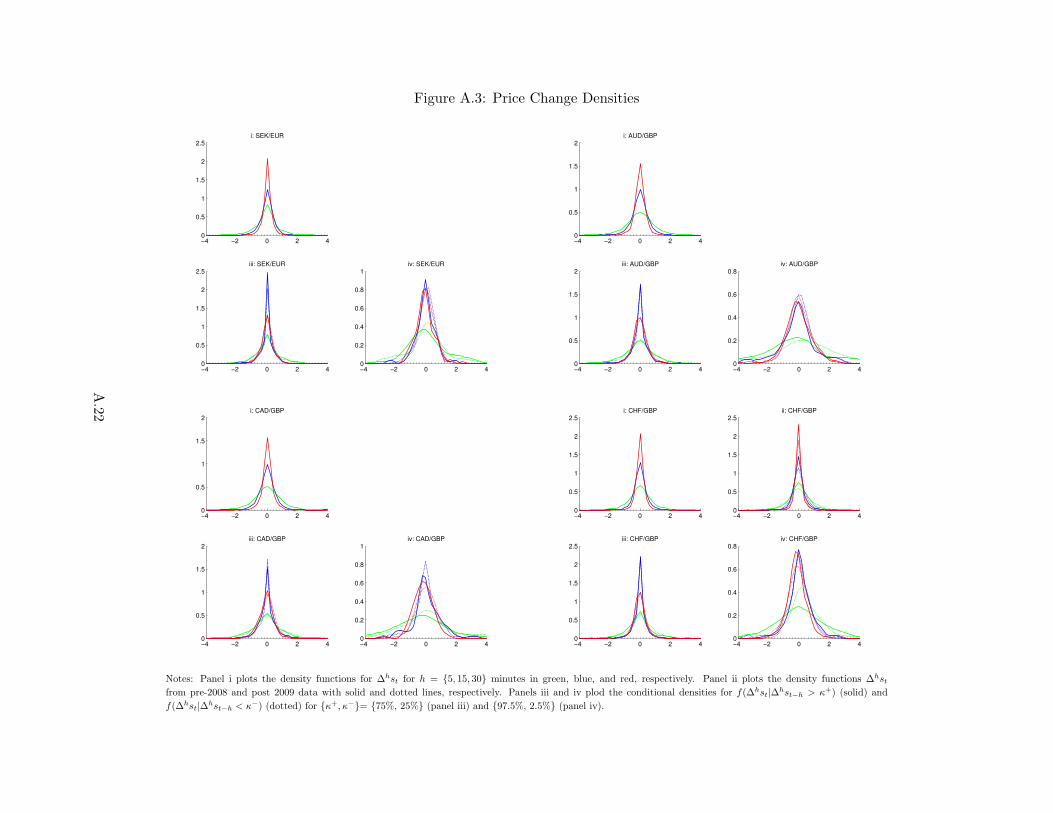
Figure A.3: Price Change Densities
−4 −2 0 2 40
0.5
1
1.5
2
2.5
i: SEK/EUR
−4 −2 0 2 40
0.5
1
1.5
2
2.5
iii: SEK/EUR
−4 −2 0 2 40
0.2
0.4
0.6
0.8
1
iv: SEK/EUR
−4 −2 0 2 40
0.5
1
1.5
2
i: AUD/GBP
−4 −2 0 2 40
0.5
1
1.5
2
iii: AUD/GBP
−4 −2 0 2 40
0.2
0.4
0.6
0.8
iv: AUD/GBP
−4 −2 0 2 40
0.5
1
1.5
2
i: CAD/GBP
−4 −2 0 2 40
0.5
1
1.5
2
iii: CAD/GBP
−4 −2 0 2 40
0.2
0.4
0.6
0.8
1
iv: CAD/GBP
−4 −2 0 2 40
0.5
1
1.5
2
2.5
i: CHF/GBP
−4 −2 0 2 40
0.5
1
1.5
2
2.5
ii: CHF/GBP
−4 −2 0 2 40
0.5
1
1.5
2
2.5
iii: CHF/GBP
−4 −2 0 2 40
0.2
0.4
0.6
0.8
iv: CHF/GBP
Notes: Panel i plots the density functions for ∆hst for h = 5, 15, 30 minutes in green, blue, and red, respectively. Panel ii plots the density functions ∆
hstfrom pre-2008 and post 2009 data with solid and dotted lines, respectively. Panels iii and iv plod the conditional densities for f(∆hst|∆
hst−h > κ+) (solid) and
f(∆hst|∆hst−h < κ−) (dotted) for κ+,κ−= 75%, 25% (panel iii) and 97.5%, 2.5% (panel iv).
A.22

Figure A.4: Price Change Densities
−4 −2 0 2 40
0.5
1
1.5
2
2.5
i: GBP/EUR
−4 −2 0 2 40
0.5
1
1.5
2
2.5
3
ii: GBP/EUR
−4 −2 0 2 40
0.5
1
1.5
2
2.5
3
iii: GBP/EUR
−4 −2 0 2 40
0.5
1
1.5
iv: GBP/EUR
−4 −2 0 2 40
0.5
1
1.5
2
i: JPY/GBP
−4 −2 0 2 40
0.5
1
1.5
2
ii: JPY/GBP
−4 −2 0 2 40
0.5
1
1.5
2
iii: JPY/GBP
−4 −2 0 2 40
0.2
0.4
0.6
0.8
iv: JPY/GBP
−4 −2 0 2 40
0.5
1
1.5
i: NZD/GBP
−4 −2 0 2 40
0.5
1
1.5
2
iii: NZD/GBP
−4 −2 0 2 40
0.2
0.4
0.6
0.8
iv: NZD/GBP
−4 −2 0 2 40
0.5
1
1.5
2
i: AUD/USD
−4 −2 0 2 40
0.5
1
1.5
2
ii: AUD/USD
−4 −2 0 2 40
0.5
1
1.5
2
iii: AUD/USD
−4 −2 0 2 40
0.2
0.4
0.6
0.8
iv: AUD/USD
Notes: Panel i plots the density functions for ∆hst for h = 5, 15, 30 minutes in green, blue, and red, respectively. Panel ii plots the density functions ∆
hstfrom pre-2008 and post 2009 data with solid and dotted lines, respectively. Panels iii and iv plod the conditional densities for f(∆hst|∆
hst−h > κ+) (solid) and
f(∆hst|∆hst−h < κ−) (dotted) for κ+,κ−= 75%, 25% (panel iii) and 97.5%, 2.5% (panel iv).
A.23

Figure A.5: Price Change Densities
−4 −2 0 2 40
0.5
1
1.5
2
2.5
i: CAD/USD
−4 −2 0 2 40
0.5
1
1.5
2
2.5
ii: CAD/USD
−4 −2 0 2 40
0.5
1
1.5
2
2.5
iii: CAD/USD
−4 −2 0 2 40
0.2
0.4
0.6
0.8
1
iv: CAD/USD
−4 −2 0 2 40
0.5
1
1.5
2
i: DKK/USD
−4 −2 0 2 40
0.5
1
1.5
2
iii: DKK/USD
−4 −2 0 2 40
0.2
0.4
0.6
0.8
1
iv: DKK/USD
−4 −2 0 2 40
0.5
1
1.5
i: NOK/USD
−4 −2 0 2 40
0.5
1
1.5
iii: NOK/USD
−4 −2 0 2 40
0.2
0.4
0.6
0.8
iv: NOK/USD
−4 −2 0 2 40
0.5
1
1.5
2
i: CHF/USD
−4 −2 0 2 40
0.5
1
1.5
2
2.5
ii: CHF/USD
−4 −2 0 2 40
0.5
1
1.5
2
iii: CHF/USD
−4 −2 0 2 40
0.2
0.4
0.6
0.8
1
iv: CHF/USD
Notes: Panel i plots the density functions for ∆hst for h = 5, 15, 30 minutes in green, blue, and red, respectively. Panel ii plots the density functions ∆
hstfrom pre-2008 and post 2009 data with solid and dotted lines, respectively. Panels iii and iv plod the conditional densities for f(∆hst|∆
hst−h > κ+) (solid) and
f(∆hst|∆hst−h < κ−) (dotted) for κ+,κ−= 75%, 25% (panel iii) and 97.5%, 2.5% (panel iv).
A.24

Figure A.6: Price Change Densities
−4 −2 0 2 40
1
2
3
4
i: SGD/USD
−4 −2 0 2 40
1
2
3
4
iii: SGD/USD
−4 −2 0 2 40
0.5
1
1.5
2
iv: SGD/USD
Notes: Panel i plots the density functions for ∆hst for h = 5, 15, 30 minutes in green, blue, and red, respectively. Panel ii plots the density functions ∆
hstfrom pre-2008 and post 2009 data with solid and dotted lines, respectively. Panels iii and iv plod the conditional densities for f(∆hst|∆
hst−h > κ+) (solid) and
f(∆hst|∆hst−h < κ−) (dotted) for κ+,κ−= 75%, 25% (panel iii) and 97.5%, 2.5% (panel iv).
A.25

Figure A.7: Pre-Fix Price Change Densities
−100 −50 0 50 1000
0.01
0.02
0.03
0.04
EUR/USD 60 mins
−50 0 500
0.02
0.04
0.06
0.08
0.1
EUR/USD 15 mins
−20 −10 0 10 200
0.05
0.1
0.15
0.2
EUR/USD 5 mins
−20 −10 0 10 200
0.1
0.2
0.3
0.4
EUR/USD 1 min
−100 −50 0 50 1000
0.01
0.02
0.03
0.04
CHF/USD 60 mins
−50 0 500
0.02
0.04
0.06
0.08
CHF/USD 15 mins
−20 −10 0 10 200
0.02
0.04
0.06
0.08
0.1
0.12
CHF/USD 5 mins
−20 −10 0 10 200
0.1
0.2
0.3
0.4
CHF/USD 1 min
−100 −50 0 50 1000
0.01
0.02
0.03
0.04
0.05
JPY/USD 60 mins
−50 0 500
0.02
0.04
0.06
0.08
0.1
JPY/USD 15 mins
−20 −10 0 10 200
0.05
0.1
0.15
0.2
JPY/USD 5 mins
−20 −10 0 10 200
0.1
0.2
0.3
0.4
JPY/USD 1 min
−100 −50 0 50 1000
0.01
0.02
0.03
0.04
USD/GBP 60 mins
−50 0 500
0.02
0.04
0.06
0.08
0.1
USD/GBP 15 mins
−20 −10 0 10 200
0.05
0.1
0.15
0.2
USD/GBP 5 mins
−20 −10 0 10 200
0.1
0.2
0.3
0.4
USD/GBP 1 min
Notes: Distribution for rate changes (in basis points) away from Fixes (black), intra-month pre-Fix (blue), and end-of-month pre-Fix (red).
A.26

Figure A.8: Pre-Fix Price Change Densities
−100 −50 0 50 1000
0.02
0.04
0.06
0.08
0.1
CHF/EUR 60 mins
−50 0 500
0.05
0.1
0.15
0.2
CHF/EUR 15 mins
−20 −10 0 10 200
0.1
0.2
0.3
0.4
CHF/EUR 5 mins
−20 −10 0 10 200
0.1
0.2
0.3
0.4
0.5
CHF/EUR 1 min
−100 −50 0 50 1000
0.01
0.02
0.03
0.04
JPY/EUR 60 mins
−50 0 500
0.02
0.04
0.06
0.08
JPY/EUR 15 mins
−20 −10 0 10 200
0.02
0.04
0.06
0.08
0.1
0.12
JPY/EUR 5 mins
−20 −10 0 10 200
0.05
0.1
0.15
0.2
0.25
JPY/EUR 1 min
−100 −50 0 50 1000
0.01
0.02
0.03
0.04
NOK/EUR 60 mins
−50 0 500
0.02
0.04
0.06
0.08
0.1
NOK/EUR 15 mins
−20 −10 0 10 200
0.05
0.1
0.15
0.2
NOK/EUR 5 mins
−20 −10 0 10 200
0.2
0.4
0.6
0.8
NOK/EUR 1 min
−100 −50 0 50 1000
0.01
0.02
0.03
0.04
NZD/EUR 60 mins
−50 0 500
0.02
0.04
0.06
0.08
NZD/EUR 15 mins
−20 −10 0 10 200
0.02
0.04
0.06
0.08
0.1
NZD/EUR 5 mins
−20 −10 0 10 200
0.05
0.1
0.15
0.2
0.25
NZD/EUR 1 min
Notes: Densities of price changes (in basis points) away from Fix (black) intra-month pre-Fix (blue) and end-of-month pre-Fix (red).
A.27

Figure A.9: Pre-Fix Price Change Densities
−100 −50 0 50 1000
0.01
0.02
0.03
0.04
SEK/EUR 60 mins
−50 0 500
0.02
0.04
0.06
0.08
0.1
SEK/EUR 15 mins
−20 −10 0 10 200
0.05
0.1
0.15
0.2
SEK/EUR 5 mins
−20 −10 0 10 200
0.1
0.2
0.3
0.4
0.5
SEK/EUR 1 min
−100 −50 0 50 1000
0.01
0.02
0.03
0.04
AUD/GBP 60 mins
−50 0 500
0.02
0.04
0.06
0.08
AUD/GBP 15 mins
−20 −10 0 10 200
0.02
0.04
0.06
0.08
0.1
AUD/GBP 5 mins
−20 −10 0 10 200
0.05
0.1
0.15
0.2
0.25
AUD/GBP 1 min
−100 −50 0 50 1000
0.005
0.01
0.015
0.02
0.025
0.03
CAD/GBP 60 mins
−50 0 500
0.02
0.04
0.06
0.08
CAD/GBP 15 mins
−20 −10 0 10 200
0.02
0.04
0.06
0.08
0.1
0.12
CAD/GBP 5 mins
−20 −10 0 10 200
0.05
0.1
0.15
0.2
0.25
CAD/GBP 1 min
−100 −50 0 50 1000
0.01
0.02
0.03
0.04
CHF/GBP 60 mins
−50 0 500
0.02
0.04
0.06
0.08
0.1
CHF/GBP 15 mins
−20 −10 0 10 200
0.05
0.1
0.15
0.2
CHF/GBP 5 mins
−20 −10 0 10 200
0.1
0.2
0.3
0.4
CHF/GBP 1 min
Notes: Densities of price changes (in basis points) away from Fix (black) intra-month pre-Fix (blue) and end-of-month pre-Fix (red).
A.28

Figure A.10: Pre-Fix Price Change Densities
−100 −50 0 50 1000
0.01
0.02
0.03
0.04
0.05
GBP/EUR 60 mins
−50 0 500
0.02
0.04
0.06
0.08
0.1
GBP/EUR 15 mins
−20 −10 0 10 200
0.05
0.1
0.15
0.2
GBP/EUR 5 mins
−20 −10 0 10 200
0.1
0.2
0.3
0.4
GBP/EUR 1 min
−100 −50 0 50 1000
0.01
0.02
0.03
0.04
JPY/GBP 60 mins
−50 0 500
0.02
0.04
0.06
0.08
JPY/GBP 15 mins
−20 −10 0 10 200
0.02
0.04
0.06
0.08
0.1
0.12
JPY/GBP 5 mins
−20 −10 0 10 200
0.05
0.1
0.15
0.2
0.25
JPY/GBP 1 min
−100 −50 0 50 1000
0.005
0.01
0.015
0.02
0.025
0.03
NZD/GBP 60 mins
−50 0 500
0.01
0.02
0.03
0.04
0.05
0.06
NZD/GBP 15 mins
−20 −10 0 10 200
0.02
0.04
0.06
0.08
0.1
NZD/GBP 5 mins
−20 −10 0 10 200
0.05
0.1
0.15
0.2
NZD/GBP 1 min
−100 −50 0 50 1000
0.01
0.02
0.03
0.04
AUD/USD 60 mins
−50 0 500
0.02
0.04
0.06
0.08
AUD/USD 15 mins
−20 −10 0 10 200
0.02
0.04
0.06
0.08
0.1
0.12
AUD/USD 5 mins
−20 −10 0 10 200
0.05
0.1
0.15
0.2
0.25
AUD/USD 1 min
Notes: Densities of price changes (in basis points) away from Fix (black) intra-month pre-Fix (blue) and end-of-month pre-Fix (red).
A.29

Figure A.11: Pre-Fix Price Change Densities
−100 −50 0 50 1000
0.01
0.02
0.03
0.04
CAD/USD 60 mins
−50 0 500
0.02
0.04
0.06
0.08
0.1
CAD/USD 15 mins
−20 −10 0 10 200
0.05
0.1
0.15
0.2
CAD/USD 5 mins
−20 −10 0 10 200
0.1
0.2
0.3
0.4
CAD/USD 1 min
−100 −50 0 50 1000
0.01
0.02
0.03
0.04
DKK/USD 60 mins
−50 0 500
0.02
0.04
0.06
0.08
DKK/USD 15 mins
−20 −10 0 10 200
0.02
0.04
0.06
0.08
0.1
0.12
DKK/USD 5 mins
−20 −10 0 10 200
0.1
0.2
0.3
0.4
DKK/USD 1 min
−100 −50 0 50 1000
0.005
0.01
0.015
0.02
0.025
NOK/USD 60 mins
−50 0 500
0.01
0.02
0.03
0.04
0.05
0.06
NOK/USD 15 mins
−20 −10 0 10 200
0.02
0.04
0.06
0.08
0.1
NOK/USD 5 mins
−20 −10 0 10 200
0.05
0.1
0.15
0.2
NOK/USD 1 min
−100 −50 0 50 1000
0.005
0.01
0.015
0.02
0.025
SEK/USD 60 mins
−50 0 500
0.01
0.02
0.03
0.04
0.05
SEK/USD 15 mins
−20 −10 0 10 200
0.02
0.04
0.06
0.08
SEK/USD 5 mins
−20 −10 0 10 200
0.05
0.1
0.15
0.2
SEK/USD 1 min
Notes: Densities of price changes (in basis points) away from Fix (black) intra-month pre-Fix (blue) and end-of-month pre-Fix (red).
A.30

Figure A.12: Pre-Fix Price Change Densities
−100 −50 0 50 1000
0.02
0.04
0.06
0.08
SGD/USD 60 mins
−50 0 500
0.05
0.1
0.15
0.2
SGD/USD 15 mins
−20 −10 0 10 200
0.05
0.1
0.15
0.2
0.25
SGD/USD 5 mins
−20 −10 0 10 200
0.1
0.2
0.3
0.4
0.5
SGD/USD 1 min
Notes: Densities of price changes (in basis points) away from Fix (black) intra-month pre-Fix (blue) and end-of-month pre-Fix (red).
A.31

Figure A.13: Bivariate Pre- and Post- Fix Price Change Densities
pre
post
EUR/USD 15 mins
−40 −20 0 20 40−40
−20
0
20
40
pre
post
EUR/USD 10 mins
−20 −10 0 10 20−20
−10
0
10
20
pre
post
EUR/USD 5 mins
−20 −10 0 10 20−20
−10
0
10
20
pre
post
EUR/USD 1 mins
−10 −5 0 5 10−10
−5
0
5
10
pre
post
CHF/USD 15 mins
−40 −20 0 20 40−40
−20
0
20
40
pre
post
CHF/USD 10 mins
−20 −10 0 10 20−20
−10
0
10
20
pre
post
CHF/USD 5 mins
−20 −10 0 10 20−20
−10
0
10
20
pre
post
CHF/USD 1 mins
−10 −5 0 5 10−10
−5
0
5
10
pre
post
JPY/USD 15 mins
−40 −20 0 20 40−40
−20
0
20
40
pre
post
JPY/USD 10 mins
−20 −10 0 10 20−20
−10
0
10
20
pre
post
JPY/USD 5 mins
−20 −10 0 10 20−20
−10
0
10
20
pre
post
JPY/USD 1 mins
−10 −5 0 5 10−10
−5
0
5
10
pre
post
USD/GBP 15 mins
−40 −20 0 20 40−40
−20
0
20
40
pre
post
USD/GBP 10 mins
−20 −10 0 10 20−20
−10
0
10
20
pre
post
USD/GBP 5 mins
−20 −10 0 10 20−20
−10
0
10
20
pre
post
USD/GBP 1 mins
−10 −5 0 5 10−10
−5
0
5
10
Notes: Each plot shows the contours of the estimated bivariate density for pre- and post-Fix price changes (in basis points) over horizons of 1 to 15 minutes. The solid
line in each plot is the estimated regression line from the regression of the post-Fix price change on the pre-Fix change. All estimates are based on end-of-month data.
A.32
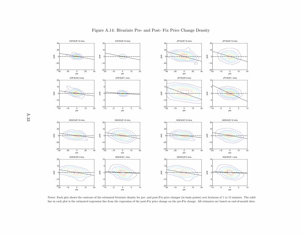
Figure A.14: Bivariate Pre- and Post- Fix Price Change Density
pre
post
CHF/EUR 15 mins
−40 −20 0 20 40−40
−20
0
20
40
pre
post
CHF/EUR 10 mins
−20 −10 0 10 20−20
−10
0
10
20
pre
post
CHF/EUR 5 mins
−20 −10 0 10 20−20
−10
0
10
20
pre
post
CHF/EUR 1 mins
−10 −5 0 5 10−10
−5
0
5
10
pre
post
JPY/EUR 15 mins
−40 −20 0 20 40−40
−20
0
20
40
pre
post
JPY/EUR 10 mins
−20 −10 0 10 20−20
−10
0
10
20
pre
post
JPY/EUR 5 mins
−20 −10 0 10 20−20
−10
0
10
20
pre
post
JPY/EUR 1 mins
−10 −5 0 5 10−10
−5
0
5
10
pre
post
NOK/EUR 15 mins
−40 −20 0 20 40−40
−20
0
20
40
pre
post
NOK/EUR 10 mins
−20 −10 0 10 20−20
−10
0
10
20
pre
post
NOK/EUR 5 mins
−20 −10 0 10 20−20
−10
0
10
20
pre
post
NOK/EUR 1 mins
−10 −5 0 5 10−10
−5
0
5
10
pre
post
NOK/EUR 15 mins
−40 −20 0 20 40−40
−20
0
20
40
pre
post
NOK/EUR 10 mins
−20 −10 0 10 20−20
−10
0
10
20
pre
post
NOK/EUR 5 mins
−20 −10 0 10 20−20
−10
0
10
20
pre
post
NOK/EUR 1 mins
−10 −5 0 5 10−10
−5
0
5
10
Notes: Each plot shows the contours of the estimated bivariate density for pre- and post-Fix price changes (in basis points) over horizons of 1 to 15 minutes. The solid
line in each plot is the estimated regression line from the regression of the post-Fix price change on the pre-Fix change. All estimates are based on end-of-month data.
A.33

Figure A.15: Bivariate Pre- and Post- Fix Price Change Density
pre
post
SEK/EUR 15 mins
−40 −20 0 20 40−40
−20
0
20
40
pre
post
SEK/EUR 10 mins
−20 −10 0 10 20−20
−10
0
10
20
pre
post
SEK/EUR 5 mins
−20 −10 0 10 20−20
−10
0
10
20
pre
post
SEK/EUR 1 mins
−10 −5 0 5 10−10
−5
0
5
10
pre
post
AUD/GBP 15 mins
−40 −20 0 20 40−40
−20
0
20
40
pre
post
AUD/GBP 10 mins
−20 −10 0 10 20−20
−10
0
10
20
pre
post
AUD/GBP 5 mins
−20 −10 0 10 20−20
−10
0
10
20
pre
post
AUD/GBP 1 mins
−10 −5 0 5 10−10
−5
0
5
10
pre
post
AUD/GBP 15 mins
−40 −20 0 20 40−40
−20
0
20
40
pre
post
AUD/GBP 10 mins
−20 −10 0 10 20−20
−10
0
10
20
pre
post
AUD/GBP 5 mins
−20 −10 0 10 20−20
−10
0
10
20
pre
post
AUD/GBP 1 mins
−10 −5 0 5 10−10
−5
0
5
10
pre
post
CHF/GBP 15 mins
−40 −20 0 20 40−40
−20
0
20
40
pre
post
CHF/GBP 10 mins
−20 −10 0 10 20−20
−10
0
10
20
pre
post
CHF/GBP 5 mins
−20 −10 0 10 20−20
−10
0
10
20
pre
post
CHF/GBP 1 mins
−10 −5 0 5 10−10
−5
0
5
10
Notes: Each plot shows the contours of the estimated bivariate density for pre- and post-Fix price changes (in basis points) over horizons of 1 to 15 minutes. The solid
line in each plot is the estimated regression line from the regression of the post-Fix price change on the pre-Fix change. All estimates are based on end-of-month data.
A.34
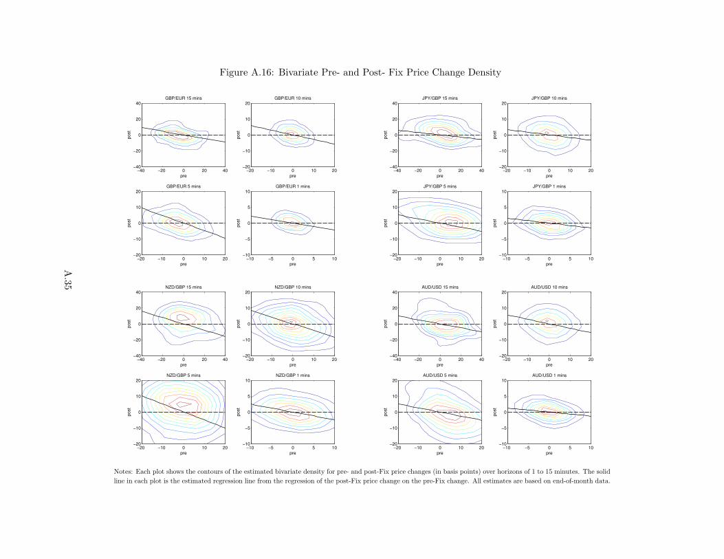
Figure A.16: Bivariate Pre- and Post- Fix Price Change Density
pre
post
GBP/EUR 15 mins
−40 −20 0 20 40−40
−20
0
20
40
pre
post
GBP/EUR 10 mins
−20 −10 0 10 20−20
−10
0
10
20
pre
post
GBP/EUR 5 mins
−20 −10 0 10 20−20
−10
0
10
20
pre
post
GBP/EUR 1 mins
−10 −5 0 5 10−10
−5
0
5
10
pre
post
JPY/GBP 15 mins
−40 −20 0 20 40−40
−20
0
20
40
pre
post
JPY/GBP 10 mins
−20 −10 0 10 20−20
−10
0
10
20
pre
post
JPY/GBP 5 mins
−20 −10 0 10 20−20
−10
0
10
20
pre
post
JPY/GBP 1 mins
−10 −5 0 5 10−10
−5
0
5
10
pre
post
NZD/GBP 15 mins
−40 −20 0 20 40−40
−20
0
20
40
pre
post
NZD/GBP 10 mins
−20 −10 0 10 20−20
−10
0
10
20
pre
post
NZD/GBP 5 mins
−20 −10 0 10 20−20
−10
0
10
20
pre
post
NZD/GBP 1 mins
−10 −5 0 5 10−10
−5
0
5
10
pre
post
AUD/USD 15 mins
−40 −20 0 20 40−40
−20
0
20
40
pre
post
AUD/USD 10 mins
−20 −10 0 10 20−20
−10
0
10
20
pre
post
AUD/USD 5 mins
−20 −10 0 10 20−20
−10
0
10
20
pre
post
AUD/USD 1 mins
−10 −5 0 5 10−10
−5
0
5
10
Notes: Each plot shows the contours of the estimated bivariate density for pre- and post-Fix price changes (in basis points) over horizons of 1 to 15 minutes. The solid
line in each plot is the estimated regression line from the regression of the post-Fix price change on the pre-Fix change. All estimates are based on end-of-month data.
A.35

Figure A.17: Bivariate Pre- and Post- Fix Price Change Density
pre
post
CAD/USD 15 mins
−40 −20 0 20 40−40
−20
0
20
40
pre
post
CAD/USD 10 mins
−20 −10 0 10 20−20
−10
0
10
20
pre
post
CAD/USD 5 mins
−20 −10 0 10 20−20
−10
0
10
20
pre
post
CAD/USD 1 mins
−10 −5 0 5 10−10
−5
0
5
10
pre
post
DKK/USD 15 mins
−40 −20 0 20 40−40
−20
0
20
40
pre
post
DKK/USD 10 mins
−20 −10 0 10 20−20
−10
0
10
20
pre
post
DKK/USD 5 mins
−20 −10 0 10 20−20
−10
0
10
20
pre
post
DKK/USD 1 mins
−10 −5 0 5 10−10
−5
0
5
10
pre
post
NOK/USD 15 mins
−40 −20 0 20 40−40
−20
0
20
40
pre
post
NOK/USD 10 mins
−20 −10 0 10 20−20
−10
0
10
20
pre
post
NOK/USD 5 mins
−20 −10 0 10 20−20
−10
0
10
20
pre
post
NOK/USD 1 mins
−10 −5 0 5 10−10
−5
0
5
10
pre
post
SEK/USD 15 mins
−40 −20 0 20 40−40
−20
0
20
40
pre
post
SEK/USD 10 mins
−20 −10 0 10 20−20
−10
0
10
20
pre
post
SEK/USD 5 mins
−20 −10 0 10 20−20
−10
0
10
20
pre
post
SEK/USD 1 mins
−10 −5 0 5 10−10
−5
0
5
10
Notes: Each plot shows the contours of the estimated bivariate density for pre- and post-Fix price changes (in basis points) over horizons of 1 to 15 minutes. The solid
line in each plot is the estimated regression line from the regression of the post-Fix price change on the pre-Fix change. All estimates are based on end-of-month data.
A.36

Figure A.18: Bivariate Pre- and Post- Fix Price Change Density
pre
post
SGD/USD 15 mins
−40 −20 0 20 40−40
−20
0
20
40
pre
post
SGD/USD 10 mins
−20 −10 0 10 20−20
−10
0
10
20
pre
post
SGD/USD 5 mins
−20 −10 0 10 20−20
−10
0
10
20
pre
post
SGD/USD 1 mins
−10 −5 0 5 10−10
−5
0
5
10
Notes: Each plot shows the contours of the estimated bivariate density for pre- and post-Fix price changes (in basis points) over horizons of 1 to 15 minutes. The solid
line in each plot is the estimated regression line from the regression of the post-Fix price change on the pre-Fix change. All estimates are based on end-of-month data.
A.37
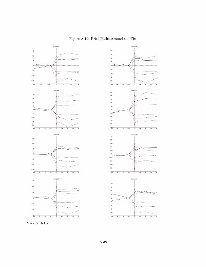
Figure A.19: Price Paths Around the Fix
−60 −40 −20 0 20 40 60
−15
−10
−5
0
5
10
15
EUR/USD
−60 −45 −30 −15 0 15 30 45 60
−20
−15
−10
−5
0
5
10
15
20
CHF/USD
−60 −45 −30 −15 0 15 30 45 60
−20
−15
−10
−5
0
5
10
15
20
JPY/USD
−60 −45 −30 −15 0 15 30 45 60−25
−20
−15
−10
−5
0
5
10
15
20
25
USD/GBP
−60 −45 −30 −15 0 15 30 45 60
−15
−10
−5
0
5
10
15
CHF/EUR
−60 −45 −30 −15 0 15 30 45 60−1
−0.8
−0.6
−0.4
−0.2
0
0.2
0.4
0.6
0.8
1
DKK/EUR
−60 −45 −30 −15 0 15 30 45 60−30
−20
−10
0
10
20
30
JPY/EUR
−60 −45 −30 −15 0 15 30 45 60
−20
−15
−10
−5
0
5
10
15
20
NOK/EUR
Notes: See below
A.38

Table A.19: Price Paths Around the Fix (cont.)
−60 −45 −30 −15 0 15 30 45 60
−30
−20
−10
0
10
20
30
NZD/EUR
−60 −45 −30 −15 0 15 30 45 60
−25
−20
−15
−10
−5
0
5
10
15
20
25
SEK/EUR
−60 −45 −30 −15 0 15 30 45 60
−30
−20
−10
0
10
20
30
AUD/GBP
−60 −45 −30 −15 0 15 30 45 60
−30
−20
−10
0
10
20
30
CAD/GBP
−60 −45 −30 −15 0 15 30 45 60
−20
−15
−10
−5
0
5
10
15
20
CHF/GBP
−60 −45 −30 −15 0 15 30 45 60
−20
−15
−10
−5
0
5
10
15
20
GBP/EUR
−60 −45 −30 −15 0 15 30 45 60
−30
−20
−10
0
10
20
30
JPY/GBP
−60 −45 −30 −15 0 15 30 45 60
−30
−20
−10
0
10
20
30
NZD/GBP
Notes: See below
A.39

Table A.19: Price Paths Around the Fix (cont.)
−60 −45 −30 −15 0 15 30 45 60
−25
−20
−15
−10
−5
0
5
10
15
20
25
AUD/USD
−60 −45 −30 −15 0 15 30 45 60
−20
−15
−10
−5
0
5
10
15
20
CAD/USD
−60 −45 −30 −15 0 15 30 45 60
−15
−10
−5
0
5
10
15
DKK/USD
−60 −45 −30 −15 0 15 30 45 60−5
−4
−3
−2
−1
0
1
2
3
4
5
HKD/USD
−60 −45 −30 −15 0 15 30 45 60
−25
−20
−15
−10
−5
0
5
10
15
20
25
NOK/USD
−60 −45 −30 −15 0 15 30 45 60−40
−30
−20
−10
0
10
20
30
40
SEK/USD
−60 −45 −30 −15 0 15 30 45 60
−8
−6
−4
−2
0
2
4
6
8
SGD/USD
Notes: Average rate path in basis points around 3:45 pm level conditioned on: (i) positive pre-Fix changes (over 15 mins) at end
of month (solid black); (ii) negative pre-Fix changes (over 15 mins) at end of month (dashed black); (iii) pre-Fix changes above the
75th. percentile of end-of-month distribution (upper red dashed dot); (iv) pre-Fix changes in the 25th. percentile of end-of-month
distribution (lower red dashed dot); (v) positive and negative pre-Fix changes on intra-month days (upper and lower blue dots).
A.40