NTNU Fakultet for naturvitenskap og teknologi Norges teknisk-naturvitenskapelige Institutt for kjemisk prosessteknologiuniversitet

SPECIALIZATION PROJECT 2013

TKP 4510

PROJECT TITLE:

Modeling of Cold Thermal Storage in Buildings

By

Emma M. Johansson

Supervisor: Sigurd Skogestad Co-supervisor: Chriss Grimholt

Date: 14.05.2013

Norwegian University of Science and TechnologyDepartment of Chemical Engineering

Specialization project fall 2012

Optimal Operation of Parallel Systems

Author:Stian Aaltvedt

Supervisors:Prof. Sigurd Skogestad

Post.doc Johannes Jäschke

December 7, 2012

Specialization project spring 2013

Modeling of Cold Thermal Storage inBuildings

Spring 2013AuthorEmma M. Johansson

SupervisorsProf. Sigurd Skogestad

Chriss Grimholt

Abstract

The goal of this project has been to study the cooling of buildings/rooms withthe use of cold thermal storage. The report presents a mathematical model of asystem that uses cold thermal storage to regulate the temperature inside a room.The system has been tested under different conditions in order to see if it thedynamics of the system are working according to the requirements.

The results from the different cases tested on the system showed that the systemworks as expected. As a result of ventilation the the indoor temperature changeswith outdoor temperature. The room gets cooled down when the radiators areturned on. The radiator temperature changes as cold water is circulating throughthe radiator and the cooling load changes as the amount of circulating waterincreases or decreases. Ice is consumed during cooling and generated when thechiller is turned on.

In order to test the system further, recommendations for further work is to includean air condition unit and optimize and regulate the system with respect to costand energy consumptions.

All simulations in the report were done using MATLAB and the built-in functionsfuntmpl.

i

Contents

Abstract i

List of Figures v

List of Tables vi

List of symbols and abbreviations vii

1 Introduction 1

2 Thermal Energy Storage 32.1 Chilled water system . . . . . . . . . . . . . . . . . . . . . . . . . . 42.2 Ice storage system . . . . . . . . . . . . . . . . . . . . . . . . . . . . 42.3 Eutectic salt storage system . . . . . . . . . . . . . . . . . . . . . . 4

3 Heat Exchangers 6

4 Model 84.1 Operational system . . . . . . . . . . . . . . . . . . . . . . . . . . . 84.2 Mass and energy balances . . . . . . . . . . . . . . . . . . . . . . . 10

5 Operational Strategy 155.1 Electric cost and rate schedules . . . . . . . . . . . . . . . . . . . . 165.2 Storage . . . . . . . . . . . . . . . . . . . . . . . . . . . . . . . . . . 18

5.2.1 Full storage . . . . . . . . . . . . . . . . . . . . . . . . . . . 195.2.2 Partial storage . . . . . . . . . . . . . . . . . . . . . . . . . 19

6 Case Studies and Results 206.1 Case 1: Inlet room and radiator temperature . . . . . . . . . . . . 226.2 Case 2: Room and radiator temperature during cooling . . . . . . . 236.3 Case 3: Massice and masswater . . . . . . . . . . . . . . . . . . . . 24

ii

6.4 Case 4: Qchiller . . . . . . . . . . . . . . . . . . . . . . . . . . . . . 266.5 Case 5: All the states, x . . . . . . . . . . . . . . . . . . . . . . . . 27

7 Discussion 30

8 Further work 33

9 Conclusion 34

References 34

A General Facts and Calculations IA.1 Varying Ventilation. . . . . . . . . . . . . . . . . . . . . . . . . . . IIA.2 Varying masssys . . . . . . . . . . . . . . . . . . . . . . . . . . . . . IVA.3 Total Amount of massice and masswater . . . . . . . . . . . . . . . . VIA.4 Varying Split Fractions . . . . . . . . . . . . . . . . . . . . . . . . . VIIA.5 Capacity of Qchiller . . . . . . . . . . . . . . . . . . . . . . . . . . . IX

B MATLAB Code and Block Digram XIB.1 MATLAB script . . . . . . . . . . . . . . . . . . . . . . . . . . . . . XIB.2 Simulink Model . . . . . . . . . . . . . . . . . . . . . . . . . . . . . XVI

iii

List of Figures

1.1 Simplified model of a cooling system with, a) no storage and b) withstorage [1] . . . . . . . . . . . . . . . . . . . . . . . . . . . . . . . . 2

3.1 A counter current heat exchanger with air and water. . . . . . . . . 6

4.1 The cooling system . . . . . . . . . . . . . . . . . . . . . . . . . . . 94.2 Dynamic model of the melting and generation of ice in the storage

tank . . . . . . . . . . . . . . . . . . . . . . . . . . . . . . . . . . . 124.3 The mixing point of the recycle flow and the return flow from the

radiator. . . . . . . . . . . . . . . . . . . . . . . . . . . . . . . . . . 13

5.1 The average energy consumption for a household during a week [2] . 175.2 The average energy consumption by the industry during a week [2]. 175.3 T basic thermal storage operating strategies ,from the left, full

storage, partial storage load leveling and partial storage demandlimiting[3]. . . . . . . . . . . . . . . . . . . . . . . . . . . . . . . . . 18

6.1 Changes in, from the top, outdoor temperature, room temperatureand radiator temperature with varying outside temperature. . . . . 22

6.2 Changes in, from the top, the room temperature, the radiator tem-peratures and split fraction. . . . . . . . . . . . . . . . . . . . . . . 24

6.3 Changes in, from the top, massice, masswater and α. . . . . . . . . . 256.4 Changes in, from the top, massice, masswater, α and Qchiller. . . . . 276.5 Changes in, from the top, room temperature, radiator temperature,

massice and masswater while changing the manipulated variables αand Qchiller. . . . . . . . . . . . . . . . . . . . . . . . . . . . . . . . 28

A.1 Changes in, from the top, outdoor temperature, room temperatureand radiator temperature with no ventilation. . . . . . . . . . . . . III

A.2 Changes in, from the top, outdoor temperature, room temperatureand radiator temperatures with different ventilations. . . . . . . . . IV

iv

A.3 Changes in, from the top, room temperature, radiator temperature,massice and masswater with varying values of masssys. . . . . . . . V

A.4 Changes in the room and radiator temperatures when outside tem-perature varies. . . . . . . . . . . . . . . . . . . . . . . . . . . . . . VII

A.5 Changes in, from the top, room temperature, radiator temperatureand α. . . . . . . . . . . . . . . . . . . . . . . . . . . . . . . . . . . VIII

A.6 Changes in, from the top, massice, masswater and α. . . . . . . . . . IXA.7 Changes in massice and masswater when changes in Qchiller. . . . . . X

v

List of Tables

1 Symbols and abbreviations . . . . . . . . . . . . . . . . . . . . . . . vii

5.1 Inequality constraints . . . . . . . . . . . . . . . . . . . . . . . . . . 16

6.1 Standard simulation parameters . . . . . . . . . . . . . . . . . . . . 216.2 Simulation variable case 2 . . . . . . . . . . . . . . . . . . . . . . . 236.3 Simulation variables case 3 . . . . . . . . . . . . . . . . . . . . . . . 256.4 Simulation variables case 4 . . . . . . . . . . . . . . . . . . . . . . . 266.5 Simulation variables case 5 . . . . . . . . . . . . . . . . . . . . . . . 28

A.1 Simulation constants [4] . . . . . . . . . . . . . . . . . . . . . . . . IA.2 Standard simulation parameters . . . . . . . . . . . . . . . . . . . . IIA.3 Simulation variables no ventilation . . . . . . . . . . . . . . . . . . IIA.4 Simulation variables changing ventilation . . . . . . . . . . . . . . . IIIA.5 Simulation parameters masssys . . . . . . . . . . . . . . . . . . . . VA.6 Simulation variables total mass . . . . . . . . . . . . . . . . . . . . VIA.7 Simulation variables split . . . . . . . . . . . . . . . . . . . . . . . . VIIA.8 Simulations variables split . . . . . . . . . . . . . . . . . . . . . . . VIIIA.9 Simulation variables Qchiller . . . . . . . . . . . . . . . . . . . . . . IX

vi

List of symbols and abbreviations

Table 1: Symbols and abbreviations

Symbol DescriptionTES Thermal energy storageCTS Cold thermal storageCFC CholorofluorocarbonCWS Chilled water systemCSTR Continuous stir tank reactorT TemperatureQ HeatU Overall heat transfer coefficientA Heat exchange aream massH EnthalpyCP Heat capacity

∆Hfus Enthalpy of fusionMfreeze Change of iceTw Freezing temp of waterα Split fraction

Vvent Air ventilationmasssys Mass circulating in the systemArad Radiator volumeVtank Volume of storage tank

vii

1 | Introduction

In a modern world like today, energy is one of the most essential needs used in dailylife. Therefore a sustainable use of energy is important such that future generationscan profit from the energy resources of the world. To run a sustainable energyconsumption energy sources should be fully utilized, unnecessary losses should beeliminated and the exploration of new energy sources investigated. One of theareas where energy utilization has been investigated is in heat exchange wherethermal energy storage (TES) has been used. In TES the energy pattern can bereshaped by storing coldness or heat in mediums when the electricity rates changesor the energy consumption can be reduced by utilizing energy that normally wouldbe wasted. One of the areas where this technology is applied is in the heating andcooling of buildings where energy needs are significant.

The energy demand of heating and cooling of buildings depends on both the geo-graphical location and the season of the year. Such as in the summertime temper-ature outside can be quite high, and the need for cooling is high, requiring energy.To be able to control the inside environment whether it is a hot or cold day aheat exchanger is necessary. Today there are several systems that can regulate theinside temperature. One sample is an air condition unit that can both control thetemperature and humidity inside or a cold thermal storage.

As already mentioned earlier the outside temperature can vary between hot andcold. This fluctuation in temperature will lead to a significant energy need in orderto keep the indoor temperature at a comfortable level, especially if the building ispoorly isolated. To be able to control the inside air to the recommended temper-atures [5], the system has to be able to meet the cooling or heating requirementsat the peak temperatures, which are the highest and coldest outdoor temperatureduring the day. This will require a system that has a high maximum capacity. Atthe off-peak periods the system is working at a lower efficiency since the tempera-ture is lower and the need for cooling is decreased. This will lead to an inefficientsystem, and a loss of money. To increase the efficiency of the system a thermalenergy storage can be used in addition to an chiller unit. A thermal energy stor-

1

which have some disadvantages, such as solidificationtemperatures of a minimum of 150 8C and corrosion effect.Molten metals (e.g. liquid sodium) can be used in theunpressurized state at temperatures of up to 760 8C withan average specific heat of 1.3 kJ/kg K [4], implying somedisadvantages, e.g. handling problems.

Rock is another good TES material from the standpoint ofcost, but its thermal capacity is only half that of water. Thepast studies showed that the rock storage bin is practical, andits main advantage is that it can easily be used for heatstorage at above 100 8C. Therefore, rocks are preferred overwater for solar systems. However, air/rock solar systems canmake provision for partial heat storage in water for domestichot water use. An amount of heat stored in rocks, comparedwith an equivalent amount of heat stored in water, occupiesapproximately three times as much space. This apparentdisadvantage is quickly overcome as soon as we comparecosts. Anyone who has built a swimming pool knows firsthand how expensive water containment can be. Addition ofthe higher cost and maintenance of a liquid collector and theeconomics quickly favor the use of air collectors with rockstorage for domestic heating applications. Combining waterwith air/rock systems has become a standard form of solarsystem application [5]. The objective is to provide a portionof energy needs for domestic hot water without a significantreduction in the solar energy supply for space heating needs.Essentially, this hybrid system is composed of a standard airrock solar system with the addition of counter-flow heatexchanger and a small water store. Conventional air/rocksolar systems for space heating see service during theheating season only. Consequently, payback time is length-ened because the solar system is inoperative for approxi-mately 6 months of the year. Adding hot water capability tothe basic air/rock system increases the capital cost by a verysmall fraction. In this respect, for a relatively slight addi-tional investment, the solar thermal system will provide100% of the domestic hot water during summer and pro-portionally less as the seasons change to and from winter.

Another example of a TES application is the use ofthermal storage to take advantage of off-peak electricitytariffs. Chiller units can be run at night when the cost ofelectricity is relatively low. These units are used to cooldown a thermal storage, which then provides cooling for

air-conditioning throughout the day. Electricity costs are notonly reduced, but also the efficiency of the chiller isincreased because of the lower night-time ambient tempera-tures, and the peak electricity demand is reduced for elec-trical supply utilities.There is a growing interest in the use of diurnal or daily

TES for electrical load management in both new and exist-ing buildings. TES technologies allow electricity consump-tion costs to be reduced by shifting electrical heating andcooling demands to periods when electricity prices arelower, for instance during the night. Load-shifting canalso reduce demand charges, which can represent a signifi-cant proportion of total electricity costs for commercialbuildings.

3. TES for cooling capacity (CTES)

In a TES for cooling capacity, ‘‘cold’’ is stored in athermal storage mass. As shown in Fig. 1, the storage canbe incorporated in an air-conditioning or cooling system in abuilding. In most conventional cooling systems, there aretwo major components [6]:

! A chiller—to cool a fluid such as water.! A distribution system—to transport the cold fluid from the

chiller to where it cools air for the building occupants.

In conventional systems, the chiller operates only whenthe building occupants require cold-air. In a cooling systemincorporating TES, the chiller also operates at times otherthan when the cooling is needed.During the past two decades, TES technology, especially

cold storage, has matured and is now accepted by many as aproven energy-conservation technology. However, the pre-dicted payback period of a potential cold storage installationis often not sufficiently attractive to give it priority over otherenergy efficient technologies. This determination often ismade because full advantage is not made of the manypotential benefits of cold storage or because the cold storagesizing is not optimized. Some recommendations for opti-mizing the payback period of CTES systems follow:For new facilities, cold storage should be integrated

carefully into the overall building and its energy systems

Fig. 1. Schematic representation of two building CTES systems: (a) with no storage and (b) with storage.

I. Dincer / Energy and Buildings 34 (2002) 377–388 379

Figure 1.1: Simplified model of a cooling system with, a) no storage and b) with storage[1]

age transfers energy from conventional energy sources, like an air condition unit,to a temperature differential in a storage medium [6], e.g a domestic hot waterheater. A TES can be divided into hot and cold storage systems depending on therequirement.

In this project the aim is to cool a room with a cold thermal storage (CTS) whenthe temperature outside is high and fluctuating. The CTS can provide the roomwith cooling during peak-hours, while the an additional cooling unit can takecare of the average cooling. The CTS can also be run with different operationalstrategies depending on what the optimal strategy is for the case where it is used.Using a CTS will lead to a decrease in the size and capacity of the chiller whilethe cooling need is still achieved [6]. Figure 1.1 show a simplified model of how anTES is used in buildings,

2

2 | Thermal Energy Storage

In the introduction a cold thermal storage was suggested as an energy utilizationwhen cooling rooms and buildings. TES systems have been used since the the1950s to store excess heat that would normally be wasted. TES examples are thestorage of ice for a space cooling in the summer and storage of heat or coolnessgenerated electrically during the off peak hours for use during the following peakhours [3]. TES can be applied to buildings where the electricity rated allow forTES to compete with other forms of cooling. The most economical benefit is foundit the buildings that have a significant cooling demand that contributes to highdemand charges [3].

CTS is a type of TES where coldness can be stored and shift electrical peak loadsas a way to manage the energy in the building. By shifting the load the energy canbe more utilized and less dependent on peak-units which have higher operatingcosts [3]. The general benefits of using CTS for the energy users, energy supplycompanies and the environment are summarized below [7]:

• reduce chiller sizes

• more efficient and effective system operations

• less capital and maintenance costs

• energy and financial savings

• reduction in carbon dioxide and CFC emissions

When implementing such a system there are several options regarding which typeof CTS should be used. In the following section some of them are presented.

3

2.1 Chilled water system

The chilled water system (CWS) contains tanks charged with cold water at tem-peratures of 4-6 ℃. The cooled water is used for the heat exchange and cooling ofthe air. The water will go from a storage tank throughout a radiator cycle whilecooling the room. As the water passes through the radiator the room heats thewater, while the cold water cools the room. The heated water then returns tothe storage tank. In ideal systems the water consists of perfect layers in the tankwith decreasing temperature towards the bottom [3]. In reality the heated waterrunning back from the heat exchanger loop will mix with the cold storage water.To minimize the mixing the heated water is supplied with low flow rates. Still thiswill decrease the cooling capacity of the CWS due to increased temperature [3].CWS also require large tank volume since each cubic meter only can provide 5.8kWh of cooling when a temperature rise of 5 ℃is used [3].

2.2 Ice storage system

In ice storage systems ice is used as a phase changing medium in addition to water,and will provide the system with more cooling capacity then chilled water systemsdue to the latent heat of fusion. In this type of system ice is generated to charge thethermal storage. When cooling is required production of ice stops and the meltingof ice provides the cooling system with cold water. In an ice storage system achiller is required for the ice building process. A chiller is an electrical unit thatproduces ice in the storage tank. The chiller is located outside of the storage tankand can either generate the ice directly from a radiator in the tank or by pipesfilled with glycol inside the tank. In the case of a glycol solution the chiller willcool the glycol to a temperature of about -6,7 ℃- 5,6 ℃. The cold glycol will thenbe pumped through the pipes and the water will freeze to ice around the coils [6].

The main benefit of thermal ice storage systems compared to conventional chilledwater systems is that an ice storage system has the ability to provide energy needsbased on time rather than cooling requirements [6].

2.3 Eutectic salt storage system

Eutectic salts are mixtures of inorganic or organic salts, water and nucleatingand stabilizing agents [3]. Eutectic mixtures have the ability to tune the freezing

4

temperature, making them lower than the individual freezing temperatures for thecomponents in the mixture [8]. The eutectic salt system is similar to ice storagein the aspect that the cooling capacity depends on the latent heat of fusion of themixture [8].

5

3 | Heat Exchangers

In order to cool or heat a room a heat exchange has to take place in order tokeep the temperature stable and at a comfortable level.The inside temperatureis affected by the natural heating or cooling of the walls from the outdoor aswell as the ventilation. Ventilation involves air exchange between the room andthe outdoor which can create substantial airspeed in the room which that cancool people and provide comfort, specially in humid areas [9]. The ventilation airentering the room often contributes to a temperature change inside the room, inaddition to the walls, which leads to the need to heat or cool the air inside tosatisfy the indoor temperature requirements. In order to do so a heat exchanger isrequired. A heat exchanger transports energy in the form of heat between media.The driving force for the heat transfer is the temperature difference between themedia [4]. The heat flows from the high temperature side to the low temperatureside to equal out the temperature difference. Figure 3.1 shows a counter currentheat exchanger with air and water on the hot and cold side, respectively.

Tinc

Touth

Tinh

Toutc

HOT SIDE

COLD SIDE

QAir

Water

Figure 3.1: A counter current heat exchanger with air and water.

When heat gets transferred from one medium to another there are three basic heattransfer mechanisms [4]:

• Conduction

• Convection

6

• Radiation

Of these mechanisms most industrial processes use conduction [10]. In this projectthe heat transfer will also be according to this mechanism. In this system thecold water will flow through pipelines to a heat exchanger, radiator, where heattransfers trough the metallic element of the radiator which is made of steel. The airwill be on the other side of the heat exchanger, shown in Figure 3.1. The radiatorwill thus cool the air in the room in addition to a conventional air condition system.

The energy transferred from the hot to the cold side in Figure 3.1 is Q. Whenassuming constant temperatures on the hot and cold sides, the heat transfer canbe calculated by Equation (3.1) [10].

Q = UA∆T (3.1)

∆T = Th − Tc, A is the heat exchange area and U is the overall heat transfercoefficient.

Usually the temperature will not be constant throughout the heat exchanger, andthe ∆T in Equation (3.1) can be replaced by the mean temperature difference[10]. The mean temperature difference is presented in Equation (3.2) where ∆T1and ∆T2 are the temperature differences for the two inlet and outlets of the heatexchanger, respectively [10].

∆T = ∆T1 −∆T2

2 (3.2)

7

4 | Model

4.1 Operational system

In this project the system is defined as a room that needs to be cooled down due tohigh outdoor temperatures. The outdoor temperatures vary during the day as thesun rises and sets, and the cooling load has to be continuously adjusted in order tokeep the inside temperature at a comfortable level. To regulate the temperatureof the room a TES is used. Of the TESs available an ice storage system is chosenbecause it is easier to control than an eutectic salt system and requires less storagevolume than a CWS.

A simplified process sheet for the system is presented in Figure 4.1. The roomis assumed to be a perfectly mixed CSTR with an inlet and outlet stream (ven-tilation). The inlet air cannot be controlled and will be a disturbance as well asan input to the system. The outlet temperature will have the same temperatureas the room, assuming perfect mixing. The size of the room is set to be 100 m3

and well isolated. In the room there are radiators that will cool the room downif the temperature reaches set level. The radiators are steel radiators with a coldcirculating water stream inside. The radiators are provided with water from aCTS and the amount of cold water entering the radiator is controlled either by asplit or by the pump from the storage tank, see Figure 4.1. The water from thestorage tank that enters the radiator first goes through a pump that sends thewater into the cooling system. The water enters a split that controls the fractionof water circulating through the radiator. If the split fraction, α, is less thanone some of the water moves through the radiators, whereas the rest circulatesback to the tank. If α is equal to zero all of the water is circulated in the chillerloop and no cooling will be applied to the room. When the water has circulatedthrough the radiator it returns to the storage tank. Before entering the tank thestream from the radiators gets mixed with the recycle stream. The temperaturewill now be a mixed temperature of the recycled stream and the stream from theradiators. This stream then continues to the tank. When entering the tank the

8

stream is carefully poured into the tank in order to prevent mixing of the fluid inthe tank. The pipelines the water flows trough and the storage tank are assumedto be well isolated. The radiators in the room are also assumed perfectly mixed.With both the room and radiator perfectly mixed the system has constant coldand hot temperatures and Equation (3.1) can be used for the system.

Figure 4.1: The cooling system

When the room is not in need of cooling ice will be generated in the ice storage bythe Qchiller. Qchiller is an electrical cooling unit (reservoir) for the ice production.Often this is a glycol solution circuit that has a temperature below the freezingpoint of water (0 ℃) [6] which will flow through pipelines in the tank and freeze thewater. In this system it is assumed to be an electrical reservoir that gets turnedon and off depending on the operating hours of the ice storage system.

9

4.2 Mass and energy balances

The model is based on the general mass balance, Equation (4.2), and energybalance, Equation (4.3), for the states of the system. The four states are theprimary variables and are presented in Equation (4.1).

x =

TroomTradiatormassicemasswater

(4.1)

The general mass equation for an open system, Equation (4.2), includes massinto and out of the system massin and massout, generated mass in the system,massgenerated, and consumed mass, massconsumed [10].

dmroom

dt= min −mout +mgenerated −mconsumed (4.2)

The general energy balance for an open system, Equation 4.3, includes enthalpy,H and heat [10]. The kinetic and potential energy are assumed to be low and aretherefore neglected in the equation. These two general mass and energy equationare used for the respective states from Equation (4.4) through (4.20).

dH

dt= Hin −Hout +Q (4.3)

The mass and engery balances for the room i presented below by Equations (4.4)through (4.7).

dmroom

dt= mroomin

−mroom−out (4.4)

The ventilation is assumed constant so there will not be any accumulation of airin the room.

mroomin= mroomout (4.5)

10

=⇒ dmroom

dt= 0 (4.6)

mroomCP,airdTroomdt

= mroominCP,airTroomin

−mroomoutCP,airTroomout−Qroom (4.7)

The balances for the radiator are presented below in Equations (4.8) through(4.11).

dmrad

dt= mradin

−mradout (4.8)

As in the case of the room, the inlet and outlet stream of the radiator are equalin order to avoid accumulation in the radiator. The inlet stream can be controlledeither by a pump or the split from the cold storage as shown in Figure 4.1.

mradin= mradout (4.9)

=⇒ dmrad

dt= 0 (4.10)

mradCP,wdTraddt

= mradinCP,wTradin

−mradoutCP,wTradout +Qroom (4.11)

Qroom is heat transferred from the room to the radiator and is calculated by Equa-tion (4.12).

Qroom = UA∆T (4.12)

Here ∆T is the temperature difference between the hot and cold sides of the heatexchanger, ∆T= Th - Tc. A [m2] is the area of the heat transfer surface and U[W/(m2 K)] is the overall heat transfer coefficient.

11

In a heat exchanger the temperature varies with the position throughout the heatexchanger [4]. Equation (4.12) refers to a perfectly mixed solution where thereis no temperature difference within the volume. The temperature gradient is thesame throughout the whole heat exchanger. In reality this is not the case, but asa simplification in this model both the room and radiator operate as two perfectlymixed CSTRs. With this assumption the heat transfer can be simplified to theexpression in Equation (4.12).

The balances for the ice and storage tank are presented in Equations (4.13) through(4.20). For the mass balance of ice Figure 4.2 shows the dynamic model of themelting and generation of ice.

ICEm

inice

moutice

Figure 4.2: Dynamic model of the melting and generation of ice in the storage tank

dmice

dt= micein

−miceout (4.13)

dmw

dt= mwin

−mwout −Mfreeze (4.14)

Here mw is the mass water, and mwinand mwout are assumed equal.

=⇒ dmw

dt= −Mfreeze (4.15)

Mfreeze = dmice

dt

negative when meltingpositive when freezing

(4.16)

12

The energy balance for the storage tank will then be as shown in Equation (4.17).

mwCP,wdTwdt

= mwinCP,win

Twin−mwoutCP,woutTwout −Mfreeze∆Hfus (4.17)

As the ice is melting or being generated the temperature in the tank, Tw, will beconstant and Equation (4.17) will be simplified to Equation (4.18).

0 = mwinCP,win

Twin−mwoutCP,woutTwout −Mfreeze∆Hfus (4.18)

Mfreeze∆Hfus = mwinCP,win

Twin−mwoutCP,woutTwout (4.19)

This gives a change of mice, given in Equation (4.20).

dmice

dt= Mfreeze = mwin

CP,winTwin−mwoutCP,woutTwout

∆Hfus

(4.20)

The recycle stream and the heated stream from the radiator get mixed on the wayback to the storage tank, as shown in Figure 4.3.

Tw

Tradm !sys

m (1-!)sys

Tmixm sys

Figure 4.3: The mixing point of the recycle flow and the return flow from the radiator.

13

The stream Tmix will then enter the storage tank as Twinin Equation (4.20). The

steady state equations for the mixing are presented in Equation (4.21) and (4.22).

Tmixmsys = Trαmsys − (1− α)Twmsys (4.21)

Tmix = Trα + (1− α)Tw (4.22)

14

5 | Operational Strategy

When operating a cooling storage system the strategy of how to use it is important.In conventional systems (only one cooling unit) the cooling load is managed bysatisfying the cooling requirements, while thermal ice storage systems allow for themanagement of energy consuming components as well [6]. This means that it ispossible to control whether the system should use the ice storage or the additionalcooling unit for cooling .

When developing an operating strategy there are several factors that should beevaluated. The main strategy should be to use the system at it’s optimal. FromSkogestad [11] the goal of optimization is to minimize an objective function, Equa-tion (5.1), to its given constraints, Equation (5.2). In this project the object func-tion is not jet chosen, but some alternatives to look at will be the total cost, totalenergy consumption or time. The equality constraints are presented in Chapter6 from the mass balances in Chapter 4.2 while the inequality constraints for thesystem are presented in to Table 5.1.

minimize J(x, ut, d) (5.1)

Subject to equality constrains: g(x, u, d, t) = 0Subject to inequality constrains: h(x, u, d, t) ≥ 0

(5.2)

Where J is the objective function, which is a function of the states, x Equation(4.1), the manipulated variables, ut, and the disturbances, d. The manipulatedvariables also denotes the systems degrees of freedom, DOFs. In order to optimizethe system the DOFs, ut, must be assigned to specific variables. If the states, x,are eliminated by using the model equations, g, the remaining problem will be

15

Equation (5.3).

minuJ(u, d) = J(uopt, d) = Jopt(d) (5.3)

Here uopt is to be found and Jopt is the optimal value of the object function J .

Table 5.1: Inequality constraints

Constrains Description ValueTroom Temperature of the room 20 < Troom < 26 [℃][5]Tradiator Temperature in the radiator 0 ≤ Tradiator ≤ Troom [℃]massice Mass of ice 0 ≤ massice ≤ 140 [kg]masswater Mass of water 0 ≤ masswater ≤ 140 [kg]

α Split fraction 0 ≤ α ≤ 1Qchiller Chiller unit Qmin ≤ Qchiller ≤ Qmax

In order to minimize the cost function, Jopt(d)in Equation (5.3), two main factorsare important [6]. One is the electricity prices, Section 5.1, and the other is storagestrategy, Section 5.2 .

5.1 Electric cost and rate schedules

Many electrical companies have rate schedules of electricity prices that change withseason of the year and time of the day. This will cause a fluctuation in the cost ofenergy and lead to the inequality such that a kW 6= a kW. The energy units arethe same, but the time-of-use will change the value of the energy [6]. Generallylow prices of electricity occur during the night time where the energy usage islow. Times when energy consumption is low is refereed to as off-peak periods.In the day time the energy consumption is high and the generating capacity anddistribution of energy might be limited and will lead to higher prices. This timeinterval is referred to as on-peak.

Figures 5.1 and 5.2 show the average energy use during the day (and weekend) fora typical household and primary-, secondary- and tertiary industry, respectively.Figure 5.1 shows the household consumption for the whole week where the greenline represents week days while the red line represents weekend.

16

47

Økonomiske analyser 6/2008 Hvordan varierer timeforbruket av strøm i ulike sektorer?

Variasjon i strømforbruket over døgnetFor å få et bedre bilde av forskjellene i forbruksmøn-steret mellom uke og helg, viser vi i figur 2 forskjellen i gjennomsnittlig timeforbruk over døgnet for hushold-ningskundene. Husholdningene har to forbrukstopper og bruker mest strøm om morgenen og kvelden. Hus-holdningene står senere opp i helgene, og reduksjonen i forbruket midt på dagen er lavere i helgene sammenlig-net med en gjennomsnittlig ukedag.

Figur 3 viser gjennomsnittlig timeforbruk over døgnet for hele året i henholdsvis ukedager og helgedager for næringskundene.

Vi ser av venstre side i figur 3 at i sekundærnæringene starter arbeidsdagen omtrent samtidig som tertiærnæ-ringene, og har en forbrukstopp i time 9. Forbruket i se-kundærnæringene er størst og varierer mest målt i kWh per time. Også i denne figuren ser vi at primærnærin-gene har klart avvikende forbruksmønster fra de andre

Figur 1. Gjennomsnittlig døgnforbruk og døgntemperatur over året for husholdnings- og næringskunder. 2006. kWh/time, °C

0,0

0,5

1,0

1,5

2,0

2,5

3,0

3,5

4,0

1.des.

1.nov.

1.okt.

1.sep.

1.aug.

1.juli

1.juni

1.mai

1.apr.

1.mars

1.feb.

1.jan.

-15

-10

-5

0

5

10

15

20

25kWh/time

Forbruk husholdning

Temperatur

°C

1.

des.1.

nov.1.

okt.1.

sep.1.

aug.1.juli

1.juni

1.mai

1.apr.

1.mars

1.feb.

1.jan.

0

20

40

60

80

100

120

140

160

-15

-10

-5

0

5

10

15

20

25kWh/time °C

PrimærTertiær

Sekundær

Temperatur

Kilde: Skagerak Nett, Metrologisk institutt.

Figur 2. Gjennomsnittlig timeforbruk over døgnet i ukedager og helger. kWh/time

0,0

0,5

1,0

1,5

2,0

2,5

242322212019181716151413121110987654321

Ukedag

Helg

kWh/time

Time

Kilde: Skagerak Nett.

Figur 3. Gjennomsnittlig timeforbruk over døgnet i ukedager og i helgene for kunder i primær-, sekundær- og tertiærnæringene. kWh/time

0

20

40

60

80

100

120

140

160

242322212019181716151413121110987654321

Tertiær

Sekundær

Primær

kWh/time

Time

Ukedag

0

20

40

60

80

100

120

140

160

242322212019181716151413121110987654321

Tertiær

Sekundær

Primær

kWh/time Helg

Time

Kilde: Skagerak Nett.

Figure 5.1: The average energy consumption for a household during a week [2]

Figure 5.1 shows that regular households have two peaks during the day. One inthe morning around 7-12 a.m. and one in the evening between 17-24 p.m.. Duringweekends the morning peak is slightly later due to a later rise in the morning andthe consumption during the day is higher probably since people stay at home.

Figure 5.2 shows the industry sector where primary industries are represented bythe green line, the secondary by the yellow, and tertiary industries by the blue.

47

Økonomiske analyser 6/2008 Hvordan varierer timeforbruket av strøm i ulike sektorer?

Variasjon i strømforbruket over døgnetFor å få et bedre bilde av forskjellene i forbruksmøn-steret mellom uke og helg, viser vi i figur 2 forskjellen i gjennomsnittlig timeforbruk over døgnet for hushold-ningskundene. Husholdningene har to forbrukstopper og bruker mest strøm om morgenen og kvelden. Hus-holdningene står senere opp i helgene, og reduksjonen i forbruket midt på dagen er lavere i helgene sammenlig-net med en gjennomsnittlig ukedag.

Figur 3 viser gjennomsnittlig timeforbruk over døgnet for hele året i henholdsvis ukedager og helgedager for næringskundene.

Vi ser av venstre side i figur 3 at i sekundærnæringene starter arbeidsdagen omtrent samtidig som tertiærnæ-ringene, og har en forbrukstopp i time 9. Forbruket i se-kundærnæringene er størst og varierer mest målt i kWh per time. Også i denne figuren ser vi at primærnærin-gene har klart avvikende forbruksmønster fra de andre

Figur 1. Gjennomsnittlig døgnforbruk og døgntemperatur over året for husholdnings- og næringskunder. 2006. kWh/time, °C

0,0

0,5

1,0

1,5

2,0

2,5

3,0

3,5

4,0

1.des.

1.nov.

1.okt.

1.sep.

1.aug.

1.juli

1.juni

1.mai

1.apr.

1.mars

1.feb.

1.jan.

-15

-10

-5

0

5

10

15

20

25kWh/time

Forbruk husholdning

Temperatur

°C

1.

des.1.

nov.1.

okt.1.

sep.1.

aug.1.juli

1.juni

1.mai

1.apr.

1.mars

1.feb.

1.jan.

0

20

40

60

80

100

120

140

160

-15

-10

-5

0

5

10

15

20

25kWh/time °C

PrimærTertiær

Sekundær

Temperatur

Kilde: Skagerak Nett, Metrologisk institutt.

Figur 2. Gjennomsnittlig timeforbruk over døgnet i ukedager og helger. kWh/time

0,0

0,5

1,0

1,5

2,0

2,5

242322212019181716151413121110987654321

Ukedag

Helg

kWh/time

Time

Kilde: Skagerak Nett.

Figur 3. Gjennomsnittlig timeforbruk over døgnet i ukedager og i helgene for kunder i primær-, sekundær- og tertiærnæringene. kWh/time

0

20

40

60

80

100

120

140

160

242322212019181716151413121110987654321

Tertiær

Sekundær

Primær

kWh/time

Time

Ukedag

0

20

40

60

80

100

120

140

160

242322212019181716151413121110987654321

Tertiær

Sekundær

Primær

kWh/time Helg

Time

Kilde: Skagerak Nett.Figure 5.2: The average energy consumption by the industry during a week [2].

17

For the industry the secondary and tertiary industries have similar energy con-sumption levels. There is a peak during the day which starts around 7 am andends at 17 pm. The primary industry has aberrant consumption pattern. Moreenergy is used during the night than in the day, and there is an opposite patternrelative to the secondary and tertiary industries.

Both households and secondary and tertiary industries have peak periods in themorning. This will cause a large load on the power system. To avoid strainedsituations like this measures should be taken in order to move the morning peaksby using time differenced prices for the sector that can move their peak hours[2]. The energy price can be lowered at off-peak periods which will lead to adecrease in costs if the industries move their energy peak away from peak timeperiods. Another way to do it is to increase the price when the energy consumptionincreases to a specific limit [2]. In this way the peaks should disappear and theenergy consumption should be more spread out during the day.

5.2 Storage

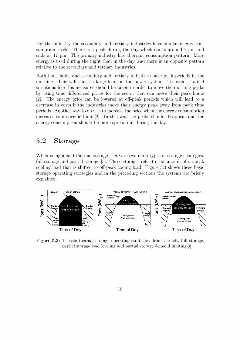
When using a cold thermal storage there are two main types of storage strategies,full storage and partial storage [3]. These storages refer to the amount of on-peakcooling load that is shifted to off-peak cooing load. Figure 5.3 shows these basicstorage operating strategies and in the preceding sections the systems are brieflyexplained.

!"## $%&'()*

!"# $%&& '()*+,# )* #&(+ $,-.%-/) '(*+(#,- ./0/./1#' ("# 2)'( )$ 2))&/0, + 3%/&4/0, 3- '"/$(/0,("# %'# )$ ("# #0#*,- $*). )0 5#+6 () )7 5#+6 ")%*' 8'## 9/,: ;<= ("#*#$)*# ("/' '(*+(#,- >/&&5*)?/4# ("# #0(/*# 4+/&- 2))&/0, *#@%/*#.#0( +( 0/,"(= 5*)?/4/0, .+A/.%. &)+4 '"/$(/0, +04 ("#"/,"#'( )5#*+(/0, 2)'( '+?/0,': !"# *#$*/,#*+(/)0 #@%/5.#0( 4)#' 0)( *%0 4%*/0, )0 5#+6 ")%*'=+04 +&& 2))&/0, &)+4' +*# .#( $*). '()*+,#: B%2" + '-'(#. *#@%/*#' *#&+(/?#&- &+*,# *#$*/,#*+(/)0+04 '()*+,# 2+5+2/(/#': 9%&& '()*+,# )5#*+(/)0 /' .)'( +((*+2(/?# >"#*# )0 5#+6 4#.+04 2"+*,#'+*# "/," )* >"#*# ("# )0 5#+6 5#*/)4 /' *#&+(/?#&- '")*(: C/(" %'# )$ ("# $%&& '()*+,# '(*+(#,-=("# 5#+6 2))&/0, #&#2(*/2 4#.+04 2)%&4 3# *#4%2#4 3- DEFGEH 2).5+*#4 >/(" + 2)0?#0(/)0+&2))&/0, '-'(#.:

0('%-(# $%&'()*

!"# 5+*(/+& '()*+,# '-'(#. .##(' + 5)*(/)0 )$ ("# )0 5#+6 2))&/0, &)+4 $*). '()*+,#= >/(" ("#*#.+/04#* )$ ("# &)+4 .#( 3- )5#*+(/)0 )$ ("# 2"/&&/0, #@%/5.#0(: I+*(/+& '()*+,# )5#*+(/0,'(*+(#,/#' 2+0 3# $%*("#* '%34/?/4#4 /0() &)+4 &#?#&/0, +04 4#.+04 &/./(/0, )5#*+(/)0: J #&(+#*1*#-/) '-'(#. (-5/2+&&- )5#*+(#' >/(" ("# *#$*/,#*+(/)0 #@%/5.#0( *%00/0, +( $%&& 2+5+2/(- $)*KL " )0 ("# 4#'/,0 4+-: C"#0 ("# 2))&/0, &)+4 /' &#'' ("+0 ("# 2"/&&#* )%(5%(= ("# #A2#'' 2))&/0,/' '()*#4M >"#0 ("# &)+4 #A2##4' ("# 2"/&&#* 2+5+2/(-= ("# +44/(/)0+& *#@%/*#.#0( /' 4/'2"+*,#4$*). '()*+,#: 9/,%*# ; /&&%'(*+(#' ("# )5#*+(/)0+& '(*+(#,- $)* + 5+*(/+& '()*+,# '-'(#.: N)+4&#?#&/0, )5#*+(/)0 /' 5+*(/2%&+*&- +((*+2(/?# $)* +55&/2+(/)0' >"#*# ("# 5#+6 2))&/0, &)+4 /' .%2""/,"#* ("+0 ("# +?#*+,# &)+4: C/(" 5+*(/+& '()*+,#= ("# 2"/&&#* /' 4)>0'/1#4 2).5+*#4 () + 2)0O?#0(/)0+& 2))&/0, '-'(#. +04 *%0' +( + '(#+4- *+(# )?#* KL ": P0 5+*(/+& '()*+,#= ("# '()*+,#*#@%/*#.#0( /' '.+&&#* ("+0 ("# )("#* '(*+(#,/#' 3#2+%'# )$ ("# 2)0(/0%)%' )5#*+(/)0 )$ ("# 2"/&O&#*: J&(")%," ("# '-'(#. )5#*+(#' 2)0(/0%)%'&- +&& 4+-= ("# '()*+,# 4)#' 0)( .##( 5#+6 4#.+04=3%( '%55&#.#0(' ("# $%&& )%(5%( )$ ("# 2"/&&#*: !"/' '(*+(#,- '+?#' +3)%( LEFQEH )$ 5#+6 2))&/0,#&#2(*/2 4#.+04: J +*2(/+ #-2-%*+ '()*+,# /' + ?+*/+(/)0 )$ 5+*(/+& '()*+,# '%2" ("+( ("# 2"/&&#**%0' 4%*/0, +&& 4+- #A2#5( ")%*' )$ .+A/.%. 0)0O2))&/0, 4#.+04 +' '")>0 /0 9/,: ;: P0 +4#.+04 &/./(#4 5+*(/+& '()*+,# '-'(#.= ("# *#$*/,#*+(/)0 #@%/5.#0( )5#*+(#' +( + *#4%2#4 2+O5+2/(- )* 4#.+04 &#?#& 4%*/0, ("# )0 5#+6 5#*/)4: !"/' '(*+(#,- *#@%/*#' 2).5&/2+(#4 2)0(*)&'-'(#.'= '/02# ("# 5#+6 4#.+04 .%'( 3# .#( ("*)%," ("# '()*+,#: !-5/2+&&-= +0 #&#2(*/2+&4#.+04 .#(#* /' %'#4 $)* ("/' 5%*5)'#: J 4#.+04 &/./(#4 '(*+(#,- /' .)'( +55&/2+3&# () 3%/&4O/0,' >/(" '/,0/R2+0( 4#.+04 2"+*,#' +04 '")*( )22%5+02- 5#*/)4' ("+( +&&)> + ,*#+(#* '()*+,#2"+*,/0, (/.#: !"# 4#.+04 &/./(/0, +55*)+2" *#5*#'#0(' + ./44&# ,*)%04 3#(>##0 &)+4 '"/$(/0,+04 &)+4 &#?#&/0,: !"# 4#.+04 '+?/0,' +' >#&& +' #@%/5.#0( 2)'(' +*# "/,"#* ("+0 (")'# $)* +&)+4 &#?#&/0, '-'(#. +04 &)>#* ("+0 (")'# $)* + &)+4 '"/$(/0, '-'(#.:

!"# 2))& '()*+,# '-'(#. 2+0 +&') 3# 2)%5&#4 >/(" '5#2/+&&- 4#'/,0#4 2)&4 +/* 4/'(*/3%(/)0 '-'O(#.'= >"/2" '%55&- 2)04/(/)0#4 +/* /0 ("# LFS!T (#.5#*+(%*# *+0,# ?#*'%' ("# ;EF;L!T *+0,#$)* 0)*.+& '-'(#.': J 2)&4 +/* 4/'(*/3%(/)0 '-'(#. 2)%5&#4 >/(" + 5+*(/+& 2))& '()*+,# '-'(#. /'+ 5+*(/2%&+*&- +((*+2(/?# /0?#'(.#0( 3#2+%'# )$ ("# *#4%2#4 2)'(' /0?)&?#4 /0 ("# *#4%2#4 +/* U)>8/:#: &#'' 4%2(>)*6 +04 '.+&&#* +/* "+04&/0, %0/('< () ("# 2)04/(/)0#4 '5+2# VK;W: P0 + 0#> 3%/&4O/0,= ("/' 2+0 +&') *#4%2# 3%/&4/0, R*'( 2)'(' 3- *#4%2/0, ("# "#/,"( 3#(>##0 U))*' +04 &)>#*/0,#&#2(*/2+& 2+3&# 2)'(': B%2" '-'(#.' "+?# +&') 3##0 '")>0 () &)>#* ("# '%..#* (/.# *#&+(/?#"%./4/(- >"/2" 5*)?/4#' 2).$)*( +( "/,"#* 4*- 3%&3 (#.5#*+(%*# '#((/0,' +04 2+0 #?#0 /.5*)?#

9/,: ;: X+'/2 ("#*.+& '()*+,# )5#*+(/0, '(*+(#,/#':

B: Y: ZJB[JP[\ ]^_P^C `[ !Z^]YJN ^[^]ab B!`]Ja^ !^TZ[`N`aP^B ;;Lc

Figure 5.3: T basic thermal storage operating strategies ,from the left, full storage,partial storage load leveling and partial storage demand limiting[3].

18

5.2.1 Full storage

Full storage or load shifting strategy divides the process in an on and off strategy.Full storage uses maximum load shifting by charging the entire daily cooling re-quirement at night and using the storage capacities during the day. While usingthe storage the refrigerating system is turned off, so the energy demand duringthe day will decrease. This strategy provides the highest operating cost savings ,but requires relatively large refrigeration and storage capacities. Figure 5.3 showshow the full storage is used [3].

5.2.2 Partial storage

Partial storage will unlike full storage not cover the whole cooling requirementwith storage only. The cooling demand will be divided between the storage andchilling equipment. Partial storage can also be divided into two categories; loadleveling and demand limiting operation [3]. A load leveling system runs withfull capacity for 24 h. When the cooling load is lower than the chiller outputthe remaining cooling will be stored, while when the cooling load is higher thethan chiller output the requirement will be met by discharging the storage [3].Figure 5.3 shows load leveling storage in the middle picture. A demand limitingsystem has a chiller that runs all the day except for hours of maximum non-coolingdemand. In this storage strategy the refrigeration equipment operates at reducedcapacity (or demand level) during the on-peak period [3]. To control this systemis complicated since the peak demand must be met by the storage. The strategyis applicable to buildings and rooms with significant demands for rapid chargingand short occupancy periods that allow for longer storage time [3].

The benefits with using partial storage in comparison with full storage is that thecosts will be lower, and the size of the chiller can be reduced [3]. In partial storagethe load leveling strategy is less expensive then the demand limiting strategy.

19

6 | Case Studies and Results

The system presented in Chapter 4.1 has been implemented in MATLAB andSimulink. The build-in function sfuntmpl has been used in all the simulations.The purpose of implementing the model in MATLAB was to see if the mathe-matical model was correct. First several simulations were done in order to getreasonable parameters for the ventilation of the system and the circulation massof the cooling circuit. The results for testing these parameters are found in theAppendix A, the values of the parameters are presented in Table 6.1 together withestimated parameters. The constants that were used are presented in Table A.1in Appendix A.

The system was tested by changing the different manipulated variables in theMATLAB file, and measuring the states in order to see if the system fulfilled itspurpose. The conditions and results for the different test are presented in Sections6.1 - 6.4. MATLAB scripts and Simulink model are to be found in Appendix B.

The equality constraints, g, of the system are presented in Equation (6.1) andare designed from the mass and energy balances in Chapter 4.2. The equalityconstraints are the same in all the case studies. The inputs of the system aredenoted as u, and Equation (6.2 )show the three inputs of the system. The statesare denoted with x and are presented in Equation (4.1).

g =

Vvent(u(1)−x(1))Vroom

− UA(x(1)−x(2))VroomCPair

ρair

masssysu(2)(Tw−x(2))Vradρwater

+ UA(x(1)−x(2))VradCPwaterρwater

u(3)∆Hfus

− masssysCPwateru(2)(x(2)−Tw)∆Hfus

masssysCPwateru(2)(x(2)−Tw)∆Hfus

− u(3)∆Hfus

(6.1)

20

u =

ToutsideαQchiller

(6.2)

Table 6.1: Standard simulation parameters

Parameters Description ValueU Overall heat transfer coefficient 0.03 [kW/(m2,K)]A Heat exchange area 1.8 [m2]Vvent Air ventilation 0.05 [m3/s]

masssys Mass circulating in the system 0.07 [m3/s]Arad Radiator volume 0.06 [m3]Vtank Storage tank volume 140 [dm3]

21

6.1 Case 1: Inlet room and radiator temperature

In the first case the room and radiator temperature were tested in order to check ifthe room temperature corresponded correctly with the outdoor temperature sincethe room is ventilated. This simulation was done with ventilation only, no cooling.The results are presented in Figure 6.1.

0 5 10 15 20

20

25

30

Outdoor temp.

Time [h]

Ou

tdo

or

tem

p.

[°C

]

0 5 10 15 2015

20

25

30

Temp. room

Time [h]

Te

mp

. ro

om

[°C

]

0 5 10 15 20

15

20

25

30Temp. radiator

Time [h]

Te

mp

. ra

dia

tor

[°C]

Figure 6.1: Changes in, from the top, outdoor temperature, room temperature andradiator temperature with varying outside temperature.

The outside temperature is around 20 ℃ in the night and increases in the morningas the sun rises. Figure 6.1 shows how the temperatures change in both the roomand radiator as the outside temperature varies. The room temperature decreasesin the beginning when the water in the radiator is still cold (the initial radiator

22

temperature is 15 ℃). After approximately an hour the temperature in the radiatoris the same as in the room then the radiator will not provide the room with coolingand the temperature in the room will increase since the outdoor temperature ishigher than the room temperature. The temperature profiles for the room andradiator are similar, but the radiator has not as distinct changes in the temperatureas the room. This result shows that the heat capacity of water is higher than forair so the heating of the radiator should be slower than the heating of the air inthe room. In addition the radiator is not exposed to the air ventilation in the samedegree as the air in the room.

6.2 Case 2: Room and radiator temperature dur-ing cooling

In case 2 cooling is applied to see if the room temperature decreases when theradiator starts to cool. The room and the radiator temperature are measured inthe simulation and should be affected by the cooling load. The cooling load of thesystem is controlled by the split fraction, α. If the split is 0, as in case 1, then allof the cooling water is circulating in the chiller loop. When the split is higher thanzero (α > 0) the water in the radiator is circulated, not only in the chiller circuit,but also through the radiator, see Figure 4.1. The results form the simulation areshown in Figure 6.2 and the manipulated variable for case 2 in Table 6.2.

Table 6.2: Simulation variable case 2

Parameters Value Timeα 0.0 0α 1.0 10

Figure 6.2 displays how the room and radiator temperatures are effected when asplit is introduced into the system. From the start the temperatures respond inthe same way as in case 1, Figure 6.1. Where the temperature decreases becausethe radiator temperature is lower then the room temperature. The splits changesfrom 0 to 1 at time 10 h, the temperature in the radiator decreases. The waterin the radiator is replaced with the cold water from the chiller loop that hasa temperature of 0 ℃. Further when the radiator temperature decreases as thewater is replaced, the room temperature also decreases. The room gets cooleddown and the temperature in the room falls with 8.8 ℃ within 3.5 hours. In theradiator the temperature drop is 19.7 ℃.

23

0 5 10 15 2010

15

20

25Temp. room

Time [h]

Te

mp

. ro

om

[°C

]

0 5 10 15 200

5

10

15

20

25Temp. radiator

Time [h]

Te

mp

. ra

dia

tor

[°C]

0 5 10 15 200

0.5

1Split fraction

Time [h]

α

Figure 6.2: Changes in, from the top, the room temperature, the radiator temperaturesand split fraction.

6.3 Case 3: Massice and masswater

In case 3 the goal was to see how the cooling affected the massice and masswater.The same simulation as in case 2 were made but with different values of α. Themanipulated variables for the simulation are presented in Table 6.3 and the resultsin Figure 6.3.

24

Table 6.3: Simulation variables case 3

Parameters Value Timeα 0.0 0α 0.5 10α 0.0 15

Qchiller 0.0 0

0 5 10 15 20

10

20

30

40

50

60Mass ice

Time [h]

Ma

ss ice

[kg

]

0 5 10 15 20

80

100

120

140

Mass water

Time [h]

Ma

ss w

ate

r [k

g]

0 5 10 15 200

0.5

1Split fraction

Time [h]

α

Figure 6.3: Changes in, from the top, massice, masswater and α.

The results presented in Figure 6.3 show how the cooling of the room changesthe amount of ice and water in the storage tank. When no cooling is applied(0-10 h and 15-24 h) both outputs are constant. When cooling (α > 0) is appliedthe amount of ice is decreasing while amount of water is increasing. In the startof the cooling, at time 10 h, the massice and masswater decreases and increases,respectively, faster than at the end of the simulation. This is because the radiatortemperature is high in the beginning when there has been no circulation in theradiator and the temperature here is the same as in the room. The hot radiator

25

temperature will increase the Tmix that goes into the storage tank and increase thespeed of melting the ice. The reason why ice is melting when cooling is applied isto produce cold water for the radiator when the need for cooling is present. Sincethe Qchiller is turned off (Qchiller = 0) there is no generated ice as the system runs.

The system in this project is a closed system, no water or ice enters or leavesthe system, the total amount of massice and masswater should be constant. FromFigure 6.3 the sum of these two are constant. A more accurate calculation is donerepresented by Figure A.4 in the Appendix A.3.

6.4 Case 4: Qchiller

In case 4 the massice and masswater were studied with both a split and a chillerunit, Qchiller. The manipulated variables used are presented in Table 6.4.

Table 6.4: Simulation variables case 4

Parameters Value Timeα 0.0 0α 0.5 5α 0. 10

Qchiller 0.0 0Qchiller 0.5 15Qchiller 0.0 20

Case 4 is a continuation of case 3. The same splits are used as in the previouscase. I addition Qchiller is turned on and off after 15 h and 20 h. The purpose ofthe simulation is to see whether Qchiller generates ice.

The results from the simulation are shown in Figure 6.4. When theQchiller is turnedon the amount of water decreases while the amount of ice increases meaning thatQchiller is generating ice. In this simplified model of cooling a room the capacity ofthe Qchiller is said to be a reservoir. In this case it is set to 1.0 kW. This results in achange of ice from 10.6 kg to 64.4 kg in 5 h. To increase the speed of generating icethe values of Qchiller can be increased to a higher value. Simulations with highercapacity on the chiller are presented in the Appendix A.5. The results show thatwith increased capacity on the chiller the amount of generated ice is increased inthe same time period.

26

0 5 10 15 20

102030405060

Mass ice

Time [h]

Ma

ss ice

[kg

]

0 5 10 15 20

80

100

120

140

Mass water

Time [h]

Ma

ss w

ate

r [k

g]

0 5 10 15 200

0.5

1Split fraction

Time [h]

α

0 5 10 15 200

1

2

3Q chiller

Time [h]

Q c

hill

er

[kW

]

Figure 6.4: Changes in, from the top, massice, masswater, α and Qchiller.

6.5 Case 5: All the states, x

As a final simulation the system was run with a cooling load and a chiller. Theaim was to see how all the states in the system correspond to each other as themanipulated variables were changed. The manipulated variables are presented inTable 6.5. The results are shown in Figure 6.5.

Figure 6.5 shows how all the states of the system changes as the manipulatedvariables are changed. The results for the indoor and radiator temperature are

27

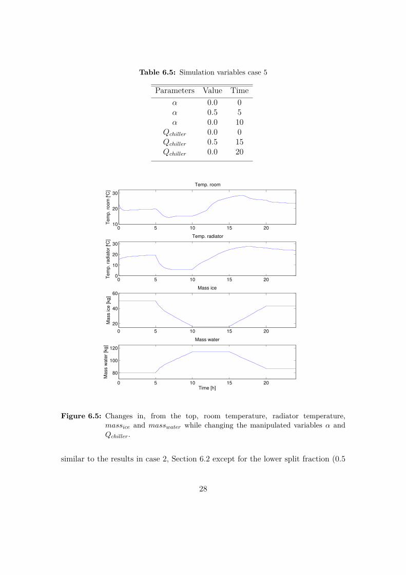
Table 6.5: Simulation variables case 5

Parameters Value Timeα 0.0 0α 0.5 5α 0.0 10

Qchiller 0.0 0Qchiller 0.5 15Qchiller 0.0 20

0 5 10 15 2010

20

30

Temp. room

Te

mp.

room

[°C

]

0 5 10 15 200

10

20

30

Temp. radiator

Tem

p. ra

dia

tor

[°C]

0 5 10 15 20

20

40

60Mass ice

Mass ice

[kg

]

0 5 10 15 20

80

100

120

Mass water

Time [h]

Mass w

ate

r [k

g]

Figure 6.5: Changes in, from the top, room temperature, radiator temperature,massice and masswater while changing the manipulated variables α andQchiller.

similar to the results in case 2, Section 6.2 except for the lower split fraction (0.5

28

compared to 1.0 in case 2), and shows how they are not affected by the chiller inthe storage tank. The massice and masswater results are the same as in case 3,and are not effected by the change in outdoor temperature.

29

7 | Discussion

The overall results from the simulation show that the system responds properlyto the changes applied. In case 1 the indoor temperature changed as a result ofventilation. The ventilation contributed to air entering the room with an othertemperature than the inside temperature. In Appendix A.1 the ventilation hasbeen further investigated. These results shows that varying the ventilation vol-ume has a direct effect on the room temperature. As the ventilation increases thetemperature in the room is more and more influenced by the outdoor tempera-ture. When the ventilation is zero the room temperature is unaffected. Theseresponses show correct behaviour to what is expected when an air exchange withdifferent temperatures is present. The temperature outside will also affect thematerial of the building. The building materials will be heated from the outsideand contribute to a temperature increase inside because of heat conduction. Thisaffect is not included in the model neither is heat contributions from people insideand interior sources as computers. If this would be included in the model theindoor temperature would be affected by four inputs, the ventilation, the walls ofthe building, the people and the interior. The ventilation is an input that can becontrolled to a certain degree as long as the air quality specifications are achieved.The heating or cooling of the building due to conduction, people and interior aresources that can not be controlled and will be a disturbance to the system. Oneway to minimize the effect of natural conduction through the walls is to isolatethe room or building. The two remaining disturbances, people and interior, areinputs that is hard to control and will be present in different degrees during the24 h circle.

The radiator temperature is also affected indirectly by the ventilation of the room.This is shown in the mass and energy balances in Chapter 4.2. Therefore, as aresult of increasing indoor temperature and no circulation in the radiator, the radi-ator temperature increases as the room temperature increases. Both the room andradiator temperature profiles follow the outdoor profile of the temperature. Theradiator profile is less defined because it is not directly affected by the ventilation,

30

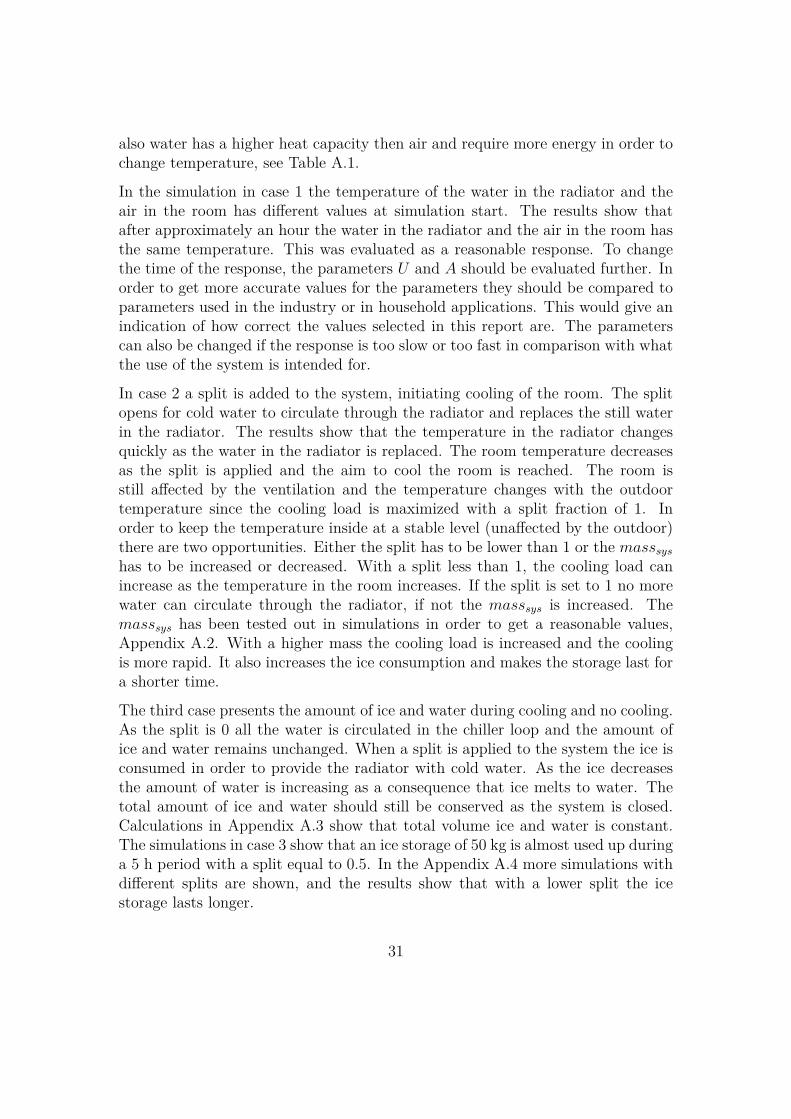
also water has a higher heat capacity then air and require more energy in order tochange temperature, see Table A.1.

In the simulation in case 1 the temperature of the water in the radiator and theair in the room has different values at simulation start. The results show thatafter approximately an hour the water in the radiator and the air in the room hasthe same temperature. This was evaluated as a reasonable response. To changethe time of the response, the parameters U and A should be evaluated further. Inorder to get more accurate values for the parameters they should be compared toparameters used in the industry or in household applications. This would give anindication of how correct the values selected in this report are. The parameterscan also be changed if the response is too slow or too fast in comparison with whatthe use of the system is intended for.

In case 2 a split is added to the system, initiating cooling of the room. The splitopens for cold water to circulate through the radiator and replaces the still waterin the radiator. The results show that the temperature in the radiator changesquickly as the water in the radiator is replaced. The room temperature decreasesas the split is applied and the aim to cool the room is reached. The room isstill affected by the ventilation and the temperature changes with the outdoortemperature since the cooling load is maximized with a split fraction of 1. Inorder to keep the temperature inside at a stable level (unaffected by the outdoor)there are two opportunities. Either the split has to be lower than 1 or the masssyshas to be increased or decreased. With a split less than 1, the cooling load canincrease as the temperature in the room increases. If the split is set to 1 no morewater can circulate through the radiator, if not the masssys is increased. Themasssys has been tested out in simulations in order to get a reasonable values,Appendix A.2. With a higher mass the cooling load is increased and the coolingis more rapid. It also increases the ice consumption and makes the storage last fora shorter time.

The third case presents the amount of ice and water during cooling and no cooling.As the split is 0 all the water is circulated in the chiller loop and the amount ofice and water remains unchanged. When a split is applied to the system the ice isconsumed in order to provide the radiator with cold water. As the ice decreasesthe amount of water is increasing as a consequence that ice melts to water. Thetotal amount of ice and water should still be conserved as the system is closed.Calculations in Appendix A.3 show that total volume ice and water is constant.The simulations in case 3 show that an ice storage of 50 kg is almost used up duringa 5 h period with a split equal to 0.5. In the Appendix A.4 more simulations withdifferent splits are shown, and the results show that with a lower split the icestorage lasts longer.

31

The fourth case show how the behaviour of Qchiller. Qchiller, affects both theamount of water and ice in the tank. As Qchiller is turned onmassice andmasswaterincreases and decreases, respectively. The result show that Qchiller generates icewhich is the goal of the chiller. In the Appendix A.5 is also tested with the aimof melting ice, and the results show that this is possible if required.

In case 5 all the states are presented in order to get an overview of all the responsesfrom the states when ventilation, cooling and Qchiller is applied. The results showthat the states corresponds the same as in the individual cases. Massice andmasswater are not affected by the ventilation and the temperature in the room andradiator are not affected by Qchiller.

32

8 | Further work

In this rapport a mathematical model for a room with a cold ice storage has beendeveloped. The model has been tested with different input parameters and theresults show that the system reacts properly to the input changes. Further workwill be to regulate and control the model. Boundaries for massice and masswaterneed to be implemented into the Simulink model to make sure that the volumesdo not become negative. An air condition unit should be added in order to testout different operating strategies, full or partial storage. In addition the systemshould be optimized with respect to either energy consumption,total costs or time.Scenarios with varying electricity prices should be optimized and a conclusion ofthe best possible solution should be presented.

The model of the heat exchange and the radiator needs to be more realistic. Inthis model both the room and radiator is said to be perfectly mixed CSTRs. Inreality there will be temperature gradients in both the radiator and the room.

In addition the temperature in the storage tank is assumed constant due to perfectmixing and constant generating of ice or melting. In reality the water can be usedin the radiator even if it does not have 0 ℃ and there should be made a dynamicmodel for increasing temperature after all ice is consumed.

33

9 | Conclusion

In this rapport a mathematical model for a room with a cold ice storage has beendeveloped. Aspects on what to consider when running the model are presented,as well as strategies.

The system has been tested in 5 cases with different values of the manipulatedvariables. The states in the system has been measured and the results analysed.The results showed that the inlet and radiator temperatures are affected by theventilation. Increasing ventilation increases the affect of the ventilation. Thetemperature in the room decreases as the radiator is turned on. The cooling loadis adjusted by amount of cold water running through the radiator. Ice is consumedduring cooling and increased cooling increases the consumption of ice. Amount ofice and water is constant. Ice is generated when the chiller in the storage tank isturned on.

The system should now be ready for a optimizing and a regulatory layer.

34

Bibliography

[1] Dincer. On thermal energy storage systems and applications in buildings.Energy and, 34:377–388, 2002.

[2] T. og B. Halvorsen Ericson. Kortsiktige svingninger i strømforbruket i almin-nelig forsyning. Forbrukskurver basert på timesmålte data fra Skagerak Nett.Statistisk sentralbyrå, 2008.

[3] S. M. Hasnain. Review on sustainable thermal energy storage technologies,part II: Cool thermal storage. Energy Convers. Mgmt, 39:1139–1153, 1998.

[4] C. J. Geankoplis. Transport Processes and searation processes principles.Pearson Education, Inc, 4 edn edition, 2003.

[5] Grønn byggallianse. Mal for Kravspesifikasjon Kontorbygg. http://www.byggalliansen.no/dokumenter/oktober_09/Mal_Kravspesifikasjon.pdf, 03 2013.

[6] EVAPO, INC. Thermal ice storage application and design guide. 5151 Allen-dale Lane, 2007.

[7] Clive Beggs. The economics of ice thermal storage. Building Research &Information, 19(6):342–355, Nov 1991.

[8] A. Abhat. Low temperature latent heat thermal energy storage: Heat storagematerials. Solar Energy, 4:313–332, 1983.

[9] J. Cook. Passiv cooling. The MIT Press, 1989.

[10] S. Skogestad. Chemical and energy process engineering. Taylor & FrancisGroup, 2009.

[11] S. Skogestad. Near-optimal operation by self-optimizingptimizing control:from process control and marathin running and business systems. Computersand Chemical Engineering, 29:127–137, 2004.

35

A | General Facts and Calcula-tions

The constants used in the simulations in the main report are presented in theMATLAB script in Appendix B, and in Table A.1 . The constants are the samein all the simulations in the project. The heat capacities are assumed constant forboth the water and air.

Table A.1: Simulation constants [4]

Constant Description Value UnitCpair Heat capacity air 1.005 [kJ/kg,K]Cpwater Heat capaity water 4.220 [kJ/kg,K]ρwater Density water 999.87 [kg/m3]ρair Density air 1.2929 [kg/m3]

∆Hfus Latent heat of fusion for water 344 [kJ/kg]

The mathematical model for the system also required some parameters for thetank, radiator and room. These parameters are presented in Table A.2. Theparameters were either tested in MATLAB in order to get reasonable values orestimated from values found in litterature.. The size of the room is an estimate ofa conference room.

I

Table A.2: Standard simulation parameters

Parameters Description Value UnitVroom Volume of the room 100 [m3]Vvent Ventilation volume 0.05 [m3/s]U Overall heat transfer coefficient 0.03 [kw/(m2,K)]A Heat exchange area 1.8 [m2]

Vtank Volume of storage tank 140 [dm3]masssys Circulation mass 0.07 [m3/s]Vradiator Volume of radiators 0.06 [m3]

A.1 Varying Ventilation.

In case 1 the room and radiator temperature were measured when no coolingwas applied while the outdoor temperature changed during the day. The roomand radiator are affected by the outdoor temperature because of the ventilation.The ventilation parameter was then tested in order to see if the affect of outdoortemperature changed as the ventilation volume changed.The specific parametersfor this simulation are shown in Table A.3. Figure A.1 displays the results fromthe simulation.

Table A.3: Simulation variables no ventilation

Parameters ValueVvent 0α 0

Figure A.1 shows that without ventilation the indoor temperature is not affectedby the outdoor temperature. Neither is the radiator temperature. Both the roomand radiator temperature changes in the first hour as the temperatures in theroom and radiator is not the same and a heat exchange takes place. When thetemperatures are equal no more heat exchange occurs.

The model was then tested with different ventilation volumes in order to see ifthe values of the parameter were reasonable and if the the room and radiatortemperatures were affected. The different values for the ventilation are presentedin Table A.4. In the main simulations in the project the air ventilation, Vvent, is0.05 m3/s. The results from the simulation are shown in Figure A.2.

As the ventilation increases the amount of air that is exchanged in the room

II

0 5 10 15 20

20

25

30

Outdoor temp.

Time [h]

Ou

tdo

or

tem

p.

[°C

]

0 5 10 15 2015

20

25

30

Temp. room

Time [h]

Te

mp

. ro

om

[°C

]

0 5 10 15 20

15

20

25

30Temp. radiator

Time [h]

Te

mp

. ra

dia

tor

[°C]

Figure A.1: Changes in, from the top, outdoor temperature, room temperature andradiator temperature with no ventilation.

Table A.4: Simulation variables changing ventilation

Parameter Value [m3/s] ColourVvent 0.02 BlueVvent 0.05 GreenVvent 0.10 Red

increases. This will influence the temperature inside the room, and indirect theradiator. The blue line in Figure A.2 represents the lowest ventilation of 0.02 m3/s,this line shows that the indoor temperature changes slowly in comparison with thered and green line which have a higher ventilation volume. When the ventilation

III

0 5 10 15 20

20

25

30

Outdoor temp.

Time [h]

Ou

tdo

or

tem

p.

[°C

]

0 5 10 15 2015

20

25

30

Temp. room

Time [h]

Te

mp

. ro

om

[°C

]

0 5 10 15 20

15

20

25

30Temp. radiator

Time [h]

Te

mp

. ra

dia

tor

[°C]

Figure A.2: Changes in, from the top, outdoor temperature, room temperature andradiator temperatures with different ventilations.

increases the indoor and radiator temperature changes more distinct as displayedwell in Figure A.2. The results with varying ventilation parameters also gives agood indication that the parameter for the ventilation in the test are reasonable.

A.2 Varying masssys

In order to see how the circulation mass,masssys influences the states in the systemsimulations were done with different masses. The different values of masssys usedin the simulations are presented in Table A.5 and the results in Figure A.3.

IV

Table A.5: Simulation parameters masssys

Parameter Value [m3/s] Colourmasssys 0.04 Redmasssys 0.07 Greenmasssys 0.10 Blue

0 5 10 15 2010

20

30

Temp. room

Te

mp

. ro

om

[°C

]

0 5 10 15 200

10

20

30

Temp. radiator

Te

mp

. ra

dia

tor

[°C]

0 5 10 15 20

20

40

60Mass ice

Ma

ss ice

[kg

]

0 5 10 15 20

80

100

120

Mass water

Time [h]

Ma

ss w

ate

r [k

g]

Figure A.3: Changes in, from the top, room temperature, radiator temperature,massice and masswater with varying values of masssys.

Figure A.3 shows how all the states are affected by the change in circulationvolume. As the volume increases the affect on all the states increases. The tem-

V

perature in the room is higher as the masssys is lower. While the temperature inthe radiator is higher as the masssys is lower. The massice is decreasing slower andmasswater increases slower. All these parameters responds correct to an decreasein cooling load as the masssys decreases. From the results in Figure A.3, 0.07 m3/was selected as a reasonable value masssys for the main simulations in the project.

A.3 Total Amount of massice and masswater

During cooling the amount of ice is decreasing while amount of water is increasing.Case 3 in the main rapport,Section 6.3 show these results. As a result of thisthe total amount of ice and water should be constant during simulation. thesimulation from case 3 was simulated again and the total values of ice and waterwere measured. The parameters used in the simulation are the same as in case 3and are presented in Table A.6. Figure A.4 shows the total amount of masswaterand massice during the simulation.

Table A.6: Simulation variables total mass

Parameters Value Timeα 0.0 0α 0.5 5α 0. 10

Qchiller 1.0 15Qchiller 0.0 20

Figure A.4 shows that the sum of massice and masswater is constant at a values of130 kg. This proves that the total amount of mass in the system is conserved.

VI

0 5 10 15 20120

122

124

126

128

130

132

134

136

138

140Total mass

Time [h]

To

tal m

ass [

kg

]

Figure A.4: Changes in the room and radiator temperatures when outside temperaturevaries.

A.4 Varying Split Fractions

In case tree in the main rapport the split was turned to 1 at time 10 h and thetemperatures both in the room and radiator decreased as a result of this. Thesplit is here tested to see if the cooling load decreases as the split decreases. Theinput parameters used here are presented in Table A.7 and the results in FigureA.5.

Table A.7: Simulation variables split

Parameters Value Time [h] Colourα 0.2 10 Redα 0.5 10 Greenα 1.0 10 Blue

When the split is decreased the amount of cooling drops. The temperature in theroom is higher as the split is lower. Which is represented by the red line in FigureA.5.

VII

0 5 10 15 2010

15

20

25Temp. room

Time [h]

Tem

p. ro

om

[°C

]

0 5 10 15 200

5

10

15

20

25Temp. radiator

Time [h]

Tem

p. ra

dia

tor

[°C]

0 5 10 15 200

0.5

1Split fraction

Time [h]

α

Figure A.5: Changes in, from the top, room temperature, radiator temperature andα.

There were also made simulations to wee how the different splits affected themassice and masswater. The parameters for the simulation are presented in TableA.8 and the results in FigureA.6.

Table A.8: Simulations variables split

Parameters Value colourα 0.2 Blueα 0.4 Greenα 0.6 Red

Figure A.6 presents the results of the massice and masswater as the cooling loadis varying with different split fractions, α. As expected the consumption of iceincreases as the cooling load increases. This also implies that masswater increasesmore rapidly.

VIII

0 5 10 15 20

10

20

30

40

50

60Mass ice

Time [h]

Ma

ss ice

[kg

]

0 5 10 15 20

80

100

120

140

Mass water

Time [h]

Ma

ss w

ate

r [k

g]

0 5 10 15 200

0.5

1Split fraction

Time [h]

α

Figure A.6: Changes in, from the top, massice, masswater and α.

A.5 Capacity of Qchiller

The capacity of the chiller was tested in order to see if it could generate ice at ahigher speed. It was also investigated to see if the Qchiller could melt ice in casethis would be needed. Simulation parameters are presented in Table A.9 and theresults in Figure A.7.

Table A.9: Simulation variables Qchiller

Parameters Value [kW?] TimeQchiller 1.0 15Qchiller -1.0 (heating) 20

Figure A.7 shows that the generation of ice increases as the capacity of Qchiller

increases. The amount of mass increases from 2.8 kg to 56.7 kg in 5 hours in

IX

0 5 10 15 20

102030405060

Mass ice

Time [h]

Ma

ss ice

[kg

]

0 5 10 15 20

80

100

120

140

Mass water

Time [h]

Ma

ss w

ate

r [k

g]

0 5 10 15 200

0.5

1Split fraction

Time [h]

α

0 5 10 15 20

−10123

Q chiller

Time [h]

Q c

hill

er

[kW

]

Figure A.7: Changes in massice and masswater when changes in Qchiller.

comparison with 29.7 kg when Qchiller was 0.5 kW. The results also shows thatQchiller is able to melt ice if this should be required (at time 22h).

X

B | MATLAB Code and Block Di-gram

The built-in function sfuntmpl was used in the simulations. Below is the MAT-LAB script sfuntmpl, Section B.1, with the state-equations. In the end the blockdiagram from Simulink is presented, Section B.2.

B.1 MATLAB script

1 %% s−function sent into the simulink model.2

3 % States:4 % x1 = Temperature of the room5 % x2 = Temperature of the radiator6 % x3 = Mass of ice7 % x4 = Mass water8

9 % Inputs:10 % u1 = Outdoor temperature11 % u2 = splitfraction12 % u3 = Q_chiller13

14 function [sys,x0,str,ts,simStateCompliance] = ...sfuntmpl(t,x,u,flag,a)

15

16 switch flag,17

18 %%%%%%%%%%%%%%%%%%19 % Initialization %20 %%%%%%%%%%%%%%%%%%21 case 0,22 [sys,x0,str,ts,simStateCompliance]=mdlInitializeSizes;

XI

23

24 %%%%%%%%%%%%%%%25 % Derivatives %26 %%%%%%%%%%%%%%%27 case 1,28 sys=mdlDerivatives(t,x,u,a);29

30 %%%%%%%%%%%%%%%%%%%%%%31 % Update & Terminate %32 %%%%%%%%%%%%%%%%%%%%%%33 case {2,9},34 sys=[]; %do nothing35

36 %%%%%%%%%%%37 % Outputs %38 %%%%%%%%%%%39 case 3,40 sys=mdlOutputs(t,x,u);41

42 otherwise43 DAStudio.error('Simulink:blocks:unhandledFlag',num2str(flag));44

45 end46

47 % end sfuntmpl48

49 %50 %================================================================51 % mdlInitializeSizes52 % Return the sizes, initial conditions,53 % and sample times for the S−function.54 %================================================================55 %56 function [sys,x0,str,ts,simStateCompliance]=mdlInitializeSizes57

58 %59 % call simsizes for a sizes structure, fill it in and convert60 %it to a sizes array.61 %62

63 sizes = simsizes;64

65 sizes.NumContStates = 4;66 sizes.NumDiscStates = 0;67 sizes.NumOutputs = 4;68 sizes.NumInputs = 3;69 sizes.DirFeedthrough = 0;70 sizes.NumSampleTimes = 1; % at least one sample time is needed71

XII

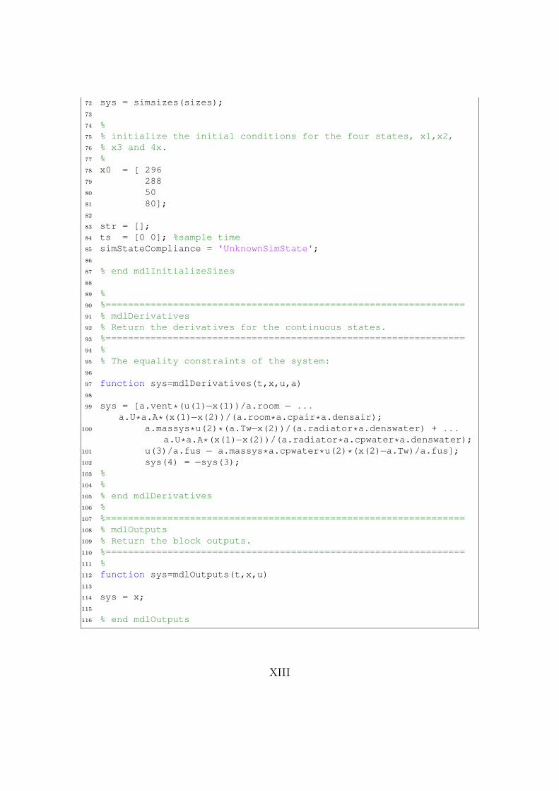
72 sys = simsizes(sizes);73

74 %75 % initialize the initial conditions for the four states, x1,x2,76 % x3 and 4x.77 %78 x0 = [ 29679 28880 5081 80];82

83 str = [];84 ts = [0 0]; %sample time85 simStateCompliance = 'UnknownSimState';86

87 % end mdlInitializeSizes88

89 %90 %================================================================91 % mdlDerivatives92 % Return the derivatives for the continuous states.93 %================================================================94 %95 % The equality constraints of the system:96

97 function sys=mdlDerivatives(t,x,u,a)98

99 sys = [a.vent*(u(1)−x(1))/a.room − ...a.U*a.A*(x(1)−x(2))/(a.room*a.cpair*a.densair);

100 a.massys*u(2)*(a.Tw−x(2))/(a.radiator*a.denswater) + ...a.U*a.A*(x(1)−x(2))/(a.radiator*a.cpwater*a.denswater);

101 u(3)/a.fus − a.massys*a.cpwater*u(2)*(x(2)−a.Tw)/a.fus];102 sys(4) = −sys(3);103 %104 %105 % end mdlDerivatives106 %107 %================================================================108 % mdlOutputs109 % Return the block outputs.110 %================================================================111 %112 function sys=mdlOutputs(t,x,u)113

114 sys = x;115

116 % end mdlOutputs

XIII

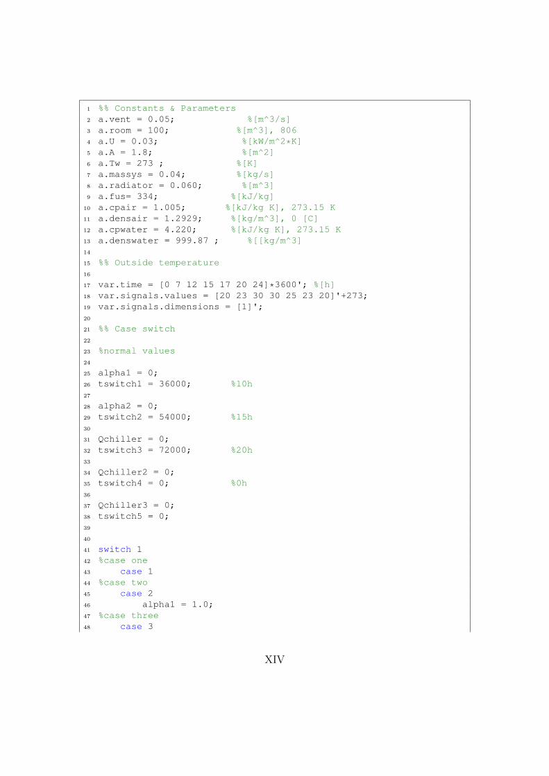
1 %% Constants & Parameters2 a.vent = 0.05; %[m^3/s]3 a.room = 100; %[m^3], 8064 a.U = 0.03; %[kW/m^2*K]5 a.A = 1.8; %[m^2]6 a.Tw = 273 ; %[K]7 a.massys = 0.04; %[kg/s]8 a.radiator = 0.060; %[m^3]9 a.fus= 334; %[kJ/kg]

10 a.cpair = 1.005; %[kJ/kg K], 273.15 K11 a.densair = 1.2929; %[kg/m^3], 0 [C]12 a.cpwater = 4.220; %[kJ/kg K], 273.15 K13 a.denswater = 999.87 ; %[[kg/m^3]14

15 %% Outside temperature16

17 var.time = [0 7 12 15 17 20 24]*3600'; %[h]18 var.signals.values = [20 23 30 30 25 23 20]'+273;19 var.signals.dimensions = [1]';20

21 %% Case switch22

23 %normal values24

25 alpha1 = 0;26 tswitch1 = 36000; %10h27

28 alpha2 = 0;29 tswitch2 = 54000; %15h30

31 Qchiller = 0;32 tswitch3 = 72000; %20h33

34 Qchiller2 = 0;35 tswitch4 = 0; %0h36

37 Qchiller3 = 0;38 tswitch5 = 0;39

40

41 switch 142 %case one43 case 144 %case two45 case 246 alpha1 = 1.0;47 %case three48 case 3

XIV

49 alpha1 = .5;50 alpha2 = −.5;51 tswitch2 = 54000;52 %case four53 case 454 alpha1 = .5;55 alpha2 = −.5;56 Qchiller = 0.5;57 Qchiller2 = −0.5;58 tswitch3 = 61200; %17h59 tswitch4 = 79200; %22h60

61

62 %case five63 case 564 alpha1 = .5;65 alpha2 = −.5;66 Qchiller = .5;67 Qchiller2 = −.5;68 tswitch1 = 18000; %5h69 tswitch2 = 36000; %10h70 tswitch3 = 54000; %15h71 tswitch4 = 72000; %20h72

73 %varying ventilation74 case 6 % Manually varying the ventilation in the paramters75

76

77 %varying mass_sys78 case 7 % Manually varying the mass_sys in the parameters79

80 %varying splits81 case 882 alpha1 = 0.2; %varying the split manually and ...

storing the values83 %alpha1 = 0.5;84 %alpha1 = 1.0;85

86 %capacity of Q_chiller87 case 988 Qchiller = 2.0;89 Qchiller2 = −3;90

91 end92

93

94 %% Simulink simulation95

96 tsim = 3600*24; %24 hour simulation over one day

XV

97

98 sim('master190413')

B.2 Simulink Model

XVI