Embed Size (px)
Citation preview

Modelling and Control of Brobekk
Waste Incineration Plant
Håvard Pehrson
Master of Science in Engineering Cybernetics
Submission date: June 2010
Supervisor: Morten Hovd, ITK
Co-supervisor: Sigurd Skogestad, IKP
Johannes Jäschke, IKP
Norwegian University of Science and Technology
Department of Engineering Cybernetics
I

II

PROBLEM DESCRIPTION
Within the Oslo district heating network, several plants are used to heat up the water
flowing through the pipe lines. One of these plants is Brobekk waste incineration plant.
Brobekk sells its produced energy to Hafslund Fjernvarme AS, which runs the district
heating network in Oslo.
This master thesis consists of studying and applying a new control structure at the
Brobekk waste incineration plant. The first part comprises a literature study and
learning how the existing process works, using a Simulink model and documentation
from Brobekk.
The second part will be to improve the Simulink model using actual measured data, so
that the model behaves more like the real process.
The final part will investigate whether it would be worthwhile applying a new type of
process control. Candidates are either a Model Predictive Control (MPC) or a Nonlinear
Model Predictive Control (NMPC). If possible, describe how to implement this in the
best way. All the simulations will be done using MATLAB/Simulink.
Assignment given: 11. January 2010
Supervisor: Morten Hovd
III

IV

ABSTRACT
Model Predictive Control of Brobekk waste incineration plant is the main focus of this
master thesis. The motivation for using MPC at Brobekk is primarily to improve the
control of the temperature towards the combustion furnace and towards Oslo.
The Brobekk plant is connected to Hafslund Fjernvarme through heat exchangers, and
where temperature and flow from Hafslund heavily affects the temperatures within the
Brobekk Plant. Based on temperature, flow and demand from Hafslund, the control
region was divided into two distinct regions, where one of the regions could be divided
in to four sub regions. Four separate Model Predictive Control structures were devised
and they were all able to successfully control the temperatures towards the combustion
furnace and towards Oslo. The transition between the two main regions was also
investigated, and the control structure developed seemed to give promising results. For
simulations, a model developed in an earlier master thesis was used. This model had to
be modified, because some physical modification had been made at Brobekk the last
year.
V

VI

PREFACE
This master thesis describes my work during the last semester at the Norwegian
University of Science and Technology. The work is carried out at the department of
Engineering Cybernetics, but the thesis is given by the Department of Chemical
Engineering and Prediktor AS.
Acknowledgements and support goes to
PhD student Johannes Jäschke at the Department of Chemical Engineering who
has been a great help during my work on this thesis. He has given me many
useful comments on the work in progress, and was always available for meetings
and discussions.
Helge Mordt at Prediktor AS who came up with this assignment and for valuable
discussion regarding Brobekk waste incineration plant, how their control system
is working today and what kind of problems they encounter with the control
system they are currently using.
Professor Morten Hovd at the Department of Engineering Cybernetics for being
kind enough to take the task as a supervisor at this thesis, even though the thesis
originally is given by the Department of Chemical Engineering.
Professor Sigurd Skogestad at the Department of Chemical Engineering for a
very interesting problem.
Finally, I want to thank my fellow students at the office; Morten Johannessen and
Torgeir Myrvold for useful discussions regarding the master thesis work and model
predictive controller. They have also been great opponents in our lunchtime card games.
Håvard Pehrson
June 2010
VII

VIII

ContentsPROBLEM DESCRIPTION.............................................................................................. III
ABSTRACT............................................................................................................................. V
PREFACE............................................................................................................................. VII
LIST OF FIGURES.............................................................................................................. XI
LIST OF TABLES............................................................................................................. XIII
ABBREVIATIONS.............................................................................................................. XV
1 INTRODUCTION........................................................................................................... 1
1.1 MOTIVATION...............................................................................................................................11.2 STRUCTURE OF THESIS............................................................................................................2
2 BACKGROUND.............................................................................................................. 3
2.1 COMPONENTS AT BROBEKK..................................................................................................32.2 OPERATIONAL ASPECTS OF BROBEKK...............................................................................52.3 CURRENT CONTROL STRUCTURE..........................................................................................6
3 MODELLING.................................................................................................................. 7
3.1 WORK DONE BY HELGE SMEDSRUD...................................................................................73.1.1 Modelling................................................................................................................................... 7
3.2 MODIFICATIONS TAKEN INTO ACCOUNT IN THIS THESIS...........................................103.2.1 Air heater................................................................................................................................ 103.2.2 Frost protection.................................................................................................................... 113.2.3 Minor adaptations made to the model.........................................................................12
3.3 INPUT DATA TO THE MODEL...............................................................................................13
4 INTRODUCTION TO MODEL PREDICTIVE CONTROL.............................15
4.1 HISTORICAL DEVELOPMENT................................................................................................164.1.1 LQG........................................................................................................................................... 16
4.2 MODEL PREDICTIVE CONTROL..........................................................................................174.2.1 The objective function........................................................................................................ 174.2.2 Internal model....................................................................................................................... 184.2.3 Control interval.................................................................................................................... 194.2.4 Prediction horizon............................................................................................................... 194.2.5 Control horizon.................................................................................................................... 194.2.6 How to choose good interval and horizons................................................................204.2.7 Constraints............................................................................................................................. 204.2.8 Infeasibility............................................................................................................................. 214.2.9 MPC Tuning........................................................................................................................... 224.2.10 Square plants and non square plants......................................................................22
4.3 NONLINEAR MPC...................................................................................................................23
IX
5 PROCESS CONTROL THEORY............................................................................25
5.1 CONTROL STRUCTURE.......................................................................................................... 255.2 CONTROL CHALLENGES OF HEAT EXCHANGERS..........................................................27
6 IMPLEMENTATION OF MPC AND SIMULATIONS......................................29
6.1 MATLAB MPC TOOLBOX.................................................................................................306.1.1 Optimization problem........................................................................................................ 306.1.2 Prediction Model................................................................................................................. 31
6.2 CONTROL CHALLENGES AT BROBEKK PLANT...............................................................326.2.1 Alpha region.......................................................................................................................... 336.2.2 Beta region............................................................................................................................. 33
6.3 CONTROL STRUCTURE DESIGN...........................................................................................386.3.1 PI controllers......................................................................................................................... 396.3.2 MPC design - Alpha region.............................................................................................426.3.3 MPC design - Beta region................................................................................................43
6.4 SIMULATIONS...........................................................................................................................436.4.1 Alpha region.......................................................................................................................... 446.4.2 Beta region............................................................................................................................. 486.4.3 Transition from alpha to beta region...........................................................................556.4.4 Transition from beta to alpha region...........................................................................58
7 CONCLUSION............................................................................................................. 63
8 BIBLIOGRAPHY......................................................................................................... 65
APPENDIX A - LIST OF SYMBOLS.............................................................................. 67
APPENDIX B - MODEL PARAMETERS.....................................................................69
APPENDIX C - OPEN LOOP STEP RESPONSES.....................................................71
X

LIST OF FIGURES
Figure 2.1: Schematic overview of the Brobekk waste incineration plant.............................4Figure 3.1: Cell model of a heat exchanger. The middle element represents the wall side separating the primary and secondary side.......................................................................................8Figure 3.2: Air heater.............................................................................................................................11Figure 3.3: Frost protection................................................................................................................. 12Figure 4.1: The difference between sampling time, prediction and control horizon.......20Figure 4.2: Process structure determines the degrees of freedom available to the controller. Adapted from Froisy (1994)..........................................................................................23Figure 5.1: Control hierarchy (Skogestad, 2004).........................................................................25Figure 5.2: Block diagram showing the two MPC alternatives...............................................27Figure 6.1: Linear model for prediction and optimization........................................................31Figure 6.2: Maximum outlet temperature, Tout as a function of flow rate............................33Figure 6.3: The different sub regions at Brobekk........................................................................35Figure 6.4: Example how the gain changes when the plant is in operation........................36Figure 6.5: Transition between different regions.........................................................................38Figure 6.6: Air temperature towards the furnace and disturbances.......................................41Figure 6.7: Temperature and flow inside air cooler....................................................................42Figure 6.8: Main flow at Brobekk.....................................................................................................42Figure 6.9: Figure (a) shows furnace inlet temperature and figure (b) shows the heat exchanger secondary side outlet temperature in the α region..................................................46Figure 6.10: Manipulated variables in the α region.....................................................................47Figure 6.11: Flow, temperature and heat demand from Hafslund in the α region............47Figure 6.12: Figure (a) shows furnace inlet temperature and figure (b) shows the heat exchanger secondary side outlet temperature in the β region alternative 1.........................50Figure 6.13: Manipulated variables in the β region alternative 1...........................................51Figure 6.14: Flow, temperature and heat demand from Hafslund in the β region............52Figure 6.15: Figure (a) shows furnace inlet temperature and figure (b) shows the heat exchanger secondary side outlet temperature in the β region alternative 2.........................53Figure 6.16: Temperature towards Oslo in the β region alternative 2...................................53Figure 6.17: Flow secondary side Heat exchanger in the β region alternative 2...............54Figure 6.18: Manipulated variables in the β region alternative 2...........................................54Figure 6.19: Figure (a) shows furnace inlet temperature and figure (b) shows the heat exchanger secondary side outlet temperature. Switching from α to β..................................56Figure 6.20: Manipulated variables. Switching from α to β.....................................................57Figure 6.21: Heat demand from Hafslund, Temperature in the Air cooler and MPC used. Switching from α to β............................................................................................................................ 58Figure 6.22: Figure (a) shows furnace inlet temperature and figure (b) shows the heat exchanger secondary side outlet temperature. Switching from β to α..................................59Figure 6.23: Manipulated variables. Switching from β to α.....................................................60Figure 6.24: Heat demand from Hafslund and MPC used. Switching from β to α..........61
XI

XII

LIST OF TABLES
Table 2.1: Manipulated variables (MVs) at Brobekk waste incineration plant....................4Table 2.2: Measured variables at Brobekk waste incineration plant........................................5Table 2.3: Main disturbances at Brobekk waste incineration plant..........................................5Table 3.1: Symbols description.............................................................................................................9Table 6.1: PI Controller parameters..................................................................................................39Table 6.2: Parameters for MPC constructed for α region..........................................................45Table 6.3: Parameters for MPC constructed for β region..........................................................48Table 6.4: Parameters for MPC constructed for β sub region 1..............................................55
XIII

XIV

ABBREVIATIONS
DHN District heating networkEGE Energigjenvinningsetaten HEN Heat Exchanger NetworkLP Linear programmingLQG Linear quadratic Gaussian controllerMPC Model predictive controlNMPC Nonlinear model predictive controllerNTU Number of transfer unitsPI(D) Proportional, integral (and derivative)QP Quadratic programmingRTO Real-time optimizerSIMC Skogestad/Simple internal model controlWIP Waste incineration plant
XV

XVI

Introduction
1 INTRODUCTION
111Equation Chapter 1 Section 1
This chapter gives a short introduction to the structure of this master thesis, as well as
an introduction to waste incineration plants.
1.1 MOTIVATION
Waste incineration plants (WIP) are widely used around the world, and with today’s
focus on climate and efficiency, the use of waste incineration plants as a source of
energy becomes increasingly interesting. When waste incineration plants burn waste,
the energy produced can be used to heat water. This heated water can then be used to
provide heat to a district heating network (DHN) through the use of heat exchangers.
Other possibilities are the production of electricity and steam.
Because of the high temperatures and pressures present in waste incineration plants it is
required to have a reliable control system. An inadequate control system may lead to
one or several conditions which all may have environmental or economical impact.
Too high temperatures may lead to pipe damage.
Too low temperatures may lead to unwanted condensation of acid and flue gas.
Too high pressure can result in rupture of valves and bends.
Too low pressure increases the risk of flashing.
Waste incineration plants may also experience grave disturbances from the district
heating network (DHN), if the temperature from the DHN is too high or the flow is too
low, both of which increases the risk of overheating and pipe-bending. On the other
hand, if the temperature from the DHN is too low and the flow is too high, the plant
may be cooled down, increasing the risk of condensation of acid and flue gas. These are
potential disturbances which place many requirements on the control system at the
waste incineration plant, where the main task for the control system is to keep the plant
within its safety limits as well as to exchange available heat efficiently.
1

Introduction
1.2 STRUCTURE OF THESIS
Chapter 2 gives a short overview of Brobekk Incineration plant, how it is connected to
Hafslund Fjernvarme, and what kind of problems they encounter with the current
control system.
Chapter 2 contains the modelling part; the chapter gives a short review of the model
which Helge Smedsrud developed in 2007/2008 and modifications made to the this
model when working with this master thesis.
Chapter 4 is included to give the reader a short insight into Model Predictive Control
(MPC) and its historical development.
Chapter 5 contains theory about process control and control challenges of heat
exchangers.
In chapter 6, the implementation and simulation using the Model Predictive Control
structure is given
And finally, chapter 7 concludes the thesis by summarizing the most important results
obtained and giving suggestions for further work to be done on the topic.
2

Background
2 BACKGROUND
212Equation Chapter (Next) Section 1
The Brobekk and Klemetsrud waste incineration plants (WIP) are operated by the Waste
recycling department of the city of Oslo (Energigjenvinningsetaten), henceforth called
EGE. This thesis concentrates on Brobekk, located at Alnabru, built in 1967 and was the
first large scale waste incineration plant in Norway. Brobekk burns waste from the
surrounding area and the energy produced is used to heat pressurized water, which heats
up water in a separate circuit through heat exchangers. This water comes from Hafslund
Fjernvarme AS, henceforth called Hafslund, which operates the district heating network
in Oslo city
The plant has been upgraded several times. In 2007, new heat exchangers were installed
and later an air heater and a frost protection system were installed.
2.1 COMPONENTS AT BROBEKK
Brobekk has two heat exchanger lines, and each line consists of several components.
A furnace, which burns the waste.
An air heater, which heats up air used in the combustion process.
An air cooler, which is used to remove excess energy when needed.
A heat exchanger that transfer heat from Brobekk to Hafslund.
Figure 2.1 shows a process diagram for one of the two heat exchanger lines at Brobekk,
as well as Hafslund’s side of the plant. The other line is not shown here, because they
are identically built up and therefore assumed to have almost the same dynamic
behaviour. The main disturbances are considered to be temperature and flow from
Hafslund. The variables are explained in Table 2.1 through Table 2.3.
3

Background
Figure 2.1: Schematic overview of the Brobekk waste incineration plant.
Table 2.1: Manipulated variables (MVs) at Brobekk waste incineration plant.
Shorthand notation Description Quantityu1 Flow pump – Brobekk 2u2 Air heater fan – Brobekk 2u3 Air cooler fan – Brobekk 2u4 Frost protection pump – Brobekk 2u5 Air heater valve – Brobekk 2u6 Bypass valve – Brobekk 2u7 Air cooler valve – Brobekk 2u8 Heat exchanger valve – Brobekk 2u9 Frost protection shutoff valve 2u10 Flow pump – Hafslund 1u11 Bypass valve – Hafslund 1u12 Heat exchanger valve – Hafslund 2
4

Background
Table 2.2: Measured variables at Brobekk waste incineration plant.
Shorthand notation
Description Quantity Unit
y1 Furnace inlet temperature 2 °Cy2 Flow to furnace 2 kg s-1
y3 Air temperature toward furnace 2 °Cy4 Air heater – Outlet temperature primary side 2 °Cy5 Air heater – Flow primary side 2 kg s-1
y6 Air cooler – Outlet temperature primary side 2 °Cy7 Air cooler – Flow primary side 2 kg s-1
y8 Heat exchanger – Outlet temperature primary side 2 °Cy9 Furnace outlet temperature 2 °Cy10 Heat exchanger – Outlet temperature secondary side 2 °Cy11 Temperature towards Oslo 1 °C
Table 2.3: Main disturbances at Brobekk waste incineration plant.
Shorthand notation Description Quantity Unitd1 Water temperature from Oslo 1 °Cd2 Flow from Oslo 1 kg s-1
2.2 OPERATIONAL ASPECTS OF BROBEKK
Each furnace at Brobekk is capable of producing 16 MW, so the total energy produced
is 32 MW. The total flow in each line is 250 tonne/h, and the furnace inlet temperature
has to be 126°C, this gives a furnace outlet temperature at 180°C. If the furnace inlet
temperature increases, the furnace outlet temperature will also increase, and if it
becomes too high, the risk of boiling in the pipes increases. In order to decrease the
furnace outlet temperature, the control system stops the fans that blow air to the furnace.
This reduces or even stops the combustions process, but it also leads to more emission
of the gas CO. It is therefore crucial that the furnace inlet temperature follows it
setpoint, within a deviation of ±3°C. This is possible through the use of either a hot
bypass or an air cooler, depending on how much energy Hafslund consumes. The
furnace inlet temperature is given by a combination of the temperatures and flows from
5

Background
the air heater, the bypass, the air cooler and the heat exchanger. Another actuating
quantity is opening and closing of valves in the plant. Because the plant is a closed
system and the total flow is 250 tonne/h, controlling a valve will affect the flow through
the other valves in the plant.
The water temperatures from Hafslund can vary between 65 to 90°C and water
temperatures that Hafslund wants towards Oslo can vary between 95°C to 110°C. The
flow rate can vary between 500 and 900 tonne/h, and is divided equally between the two
heat exchanger lines.
One of the largest problems Brobekk encounters is when Hafslund, because of less heat
needed, drastically reduces their flow towards the heat exchangers. If the heat needed
from Hafslund drops below 32 MW, Brobekk has to remove excess energy using air
coolers. When this happens it has been measured that the furnace inlet temperature,
decreases a little bit, before it increases beyond limits. These patterns seem to be valid,
and it will be the main thesis to investigate if an MPC or a nonlinear MPC can perform
better than the current control structure.
2.3 CURRENT CONTROL STRUCTURE
Today the control structure at Brobekk is divided between EGE and Hafslund, in such
way that they control their specific side of the heat exchangers: EGE controlling the
primary side and Hafslund controlling the secondary side and where the two control
systems fight each other. Intuitively, this doesn’t seem like an ideal control structure,
and it would be better to let one party control the heat exchanger. But because of
various reasons, none of the parties will give up its control structure. To make it more
confusing, both parties can also control some of the valves at both sides of the heat
exchangers, where minimum or maximum selectors are used to determine which
controller that is used for control. This makes the control system rather difficult to
understand and more complex than it needs to be.
Hafslund uses the bypass valve u11 to control the water temperature towards Oslo and
the valves u12 are used to split up the flow so that there is an equal amount of mass flow
towards each heat exchanger.
6

Modelling
3 MODELLING
313Equation Chapter (Next) Section 1This chapter gives the reader some insight to the
work done by Helge Smedsrud as well as modelling done in this master thesis.
3.1 WORK DONE BY HELGE SMEDSRUD
Master student Helge Smedsrud worked with almost the same problem description in
his master thesis from 2007/2008 (Smedsrud, 2008). He developed a model of the
Brobekk plant in Simulink and used this model to study a self-optimizing control
structure. His thesis divided the control region into 4 distinct regions, depending on
temperature and flow from Hafslund. Using a self-optimizing control approach, he
found an optimal control structure and setpoints for each region. In order to controlling
the bypass valve, heat exchanger valve, air cooler fan and valve at Brobekk’s side, it
was also necessary to control valves at Hafslund’s side of the heat exchanger.
There have been identified some weaknesses in this control structure. The first is that
Smedsrud are using valves, which EGE are not able to control; these are the valves u11
and u12 on the Hafslund side of the heat exchanger. If EGE were given control over
these valves, Hafslund would not be able to control the temperature towards Oslo and
the temperature of the hot water going to Oslo could vary a lot. Simulation results
proved that the furnace inlet temperature followed it setpoint well, but the temperature
towards Oslo varied a lot when Hafslund wanted to take out less that 32 MW. Another
weakness in this control structure is that Smedsrud is using the Bypass valve at
Hafslund side to control both the heat exchanger lines at Brobekk. From a control point
of view, it is impossible to use one manipulated variable to control two variables. He
decided to do this, because he assumed that both lines are identical, but this is unlikely
in a real situation.
3.1.1 MODELLING
For the furnaces Smedsrud uses a Number of Transfer Units or NTU method
(Hertzberg, 2008, Mathisen ,1994), which approximates a heat exchanger, but without
7

Modelling
the dynamic behaviour that is present in heat exchangers. The NTU model of the
furnace is designed such that when the flow through the furnace is 250 tonne/h and the
furnace inlet temperature is 126°C, the furnace outlet temperature is 180°C.
For the heat exchangers he uses a lumped compartment or “multi-cell” model
(Mathisen, 1994). The “multi-cell” model approximates a partial differential equation
where the heat exchanger are divided into perfectly and instantly mixing cells, where
each cell features a primary side, a wall and a secondary side element. In the model,
Smedsrud uses ten cells, all having identical properties. Figure 3.2 shows how the heat
exchangers are modelled.
Figure 3.2: Cell model of a heat exchanger. The middle element represents the wall side separating the primary and secondary side.
The ordinary differential equation is given below and symbols are described in Table 3.4.
434\*
MERGEFORMAT (.)
535\*
MERGEFORMAT (.)
636\*
MERGEFORMAT (.)
8

Modelling
Table 3.4: Symbols description.
Shorthand notation Description UnitT Temperature °Ct Time Secondh Heat transfer
coefficientW m-2 K-1
A Heat transfer area m2
w Mass flow rate kg s-1
cp Specific heat capacity J kg-1 K-1
N Number of cells -ρ Density kg m-3
V Volume m3
Superscript p, w and s denotes primary, wall and secondary side respectively.
For the fans, Smedsrud uses the Bernoulli equation where he assumes low pressure drop
across the fan and a horizontal position.
737\*MERGEFORMAT (.)
where 𝜂 is efficiency, A is area, ρ is density, w is mass flow rate, and p pressure.
The Bernoulli equation is also used for the pumps, where the elevation was set to zero,
the diameter was assumed equal before and after the pump, and the pressure after the
pump was assumed constant.
838\* MERGEFORMAT (.)
where 𝜂 is efficiency, ρ is density, w is mass flow rate, P power, and p pressure.
The valves were modelled using a standard valve equation.
9

Modelling
939\* MERGEFORMAT (.)
where Q volumetric flow rate, Kv is valve constant, ρ is density, and p is pressure.
For mixing the flows Smedsrud uses a simple expression, under the assumption of an
instant and homogeneous mixing.
Smedsrud also made some simplifications and assumptions:
Since the system only contains pressurized water and non compressed air, all
thermo dynamic and material properties like heat capacities and densities were
assumed constant and average values for the respective temperatures were used.
Pressure drops over heat exchangers were ignored, because this is very small
for modern heat exchangers
Isothermal flow was assumed through pumps, fans and valves due to the low
pressure differences in the system.
The same simplifications and assumptions were used during work with this thesis.
The reader is encouraged to read Smedsrud’s master thesis (Smedsrud, 2008) for more
detailed information about the model.
3.2 MODIFICATIONS TAKEN INTO ACCOUNT IN THIS THESIS
In 2008 and 2009, several physical modifications were implemented at Brobekk, and
these modifications had to be implemented in the model Smedsrud developed, before a
model predictive controller could be implemented. This section gives a review of these
modifications made.
3.2.1 AIR HEATER
In order to have a better and more stable burning process, it was decided to install air
heaters. The air heaters heat up air that is used in the furnace. EGE uses the heated
water produced at Brobekk to heat up the air. The air is heated to 90°C before it is fed
into the combustion process. The maximum total energy used to heat up the air is
approximately 650 kW, which is about 4 percent of the total amount of energy produced
at Brobekk.
10

Modelling
The air heater was modelled using the same heat exchanger model structure Smedsrud
used, but without the wall element and using 9 cells. The parameters were adjusted to
give correct steady state values, and are given in appendix B. A design specification on
the air heater gives a primary side outlet temperature at approximately 145°C with a
flow rate at 4.5 kg/s at the primary side and a flow rate at 6 kg/s at the secondary side.
Figure 3.3 shows the air heater.
Figure 3.3: Air heater.
3.2.2 FROST PROTECTION
The other main modification at Brobekk was the installation of the frost protection
equipment in the air cooler. This was implemented in 2008, because in December
2007/January 2008 the air cooler was damaged due to water freezing inside the air
cooler. The frost protection systems consists of a flow controller that ensures that the
flow through the air cooler always is 15.125 kg/s (60 tonne/h) and a temperature
controller that ensure that the temperature in the air cooler never comes below 10°C.
The flow controller controls a pump, which pumps water from outlet primary side to the
inlet primary side of the air cooler. The pump only operates when the outside air
temperature is below 5°C. The temperature controller controls the air cooler valve,
where hot water from the furnace is used to heat up the water temperature inside the air
cooler.
To keep the Simulink model simple, it was decided to not to model the flow controller
or the pump, instead a statement was made, where the flow driven by the pump was set
to 15.125 kg/s subtracting the flow through the air cooler valve. By making this
11

Modelling
statement, the flow through the air cooler always is 15,125 kg/s, but the flow driven the
pump can vary. If the flow through the air cooler valve is larger than 15.125 kg/s, the
flow driven by the pump is set to zero. The statement is only valid if the outside air
temperature is below 5°C. The temperature controller was modelled like a PI controller.
The frost protection system is shown in Figure 3.4.
Figure 3.4: Frost protection.
3.2.3 MINOR ADAPTATIONS MADE TO THE MODEL
Because the model developed by Smedsrud was designed for a slightly different
purpose, some minor adaptations had to be included in the model.
Flow mixersAs mentioned earlier, Smedsrud uses a simple expression below for mixing the flows. The
expression is given in equations 310 and 311
10310\* MERGEFORMAT (.)
11311\* MERGEFORMAT (.)
Consideration of equation 311 reveals that the temperature will be infinity, if the total
flow, Wtot, is equal to zero. To circumvent this, a simple statement was implemented,
12

Modelling
setting the outlet temperature, Ttot , equal to inlet temperature, if the total flow is zero.
This statement was only used when mixing the frost protection feedback flow and the
flow through the air cooler valve, because this is the only situation where the model can
have zero flow through a mixer. Zero flow through this flow mixer happens when the
frost protection system is unused, i.e. the air temperature is higher than 5°C and the air
cooler valve is closed.
Anti windup in PI controller
Anti windup was not implemented in the PI controllers Smedsrud developed. This
allowed the integral action in the PI controllers to windup, causing some
incomprehensible simulation results. The PI controllers were therefore modified to
include anti windup.
3.3 INPUT DATA TO THE MODEL
As mentioned in the problem description, one task was to use actual measured data in
order to improve the dynamic behaviour in model. In discussion with Johannes Jäschke,
it was decided not work further with this task. It was assumed that the model already
had all the similar characteristics as the real plant. Some of the gains and time constant
in the model might be different from the real plant, but it would not be worthwhile to
spend effort on this task.
13

Modelling
14

Introduction to Model Predictive Control
4 INTRODUCTION TO MODEL PREDICTIVE CONTROL
1214Equation Chapter (Next) Section 1
Predictive Control, or Model-based Predictive Control, MPC, is the only advanced
control technique – that is, more advanced than standard PID control – to have had a
significant and widespread impact on industrial processes (Maciejowski, 2002). It has
mainly been used in petrochemical industry, but has gradually gained interest in other
sectors of control engineering, such as control of airplanes and vehicles.
The main reasons for this are that MPC is (Maciejowski, 2002).
The only control technology which can deal routinely with equipment and safety
constraints.
The underlying idea is easy to understand.
Its basic formulation extends to multivariable plants with almost no
modification.
It is more powerful than PID control, even on ‘difficult’ loops such as those
containing long time delays.
The development of MPC started about 40 years ago, but it is difficult to assign the
beginning to one person or one company because the ideas seems to have been proposed
by several authors more or less simultaneously. Lee and Markus (1967) anticipated
current MPC practice in their 1967 text on optimal control:
One technique for obtaining a feedback
controller synthesis from knowledge of
open-loop controllers is to measure the
current control process state and then
compute very rapidly for the open-loop
control function. The first portion of this
function is then used during a short time
interval, after which a new measurements of
the function is computed for this new
15

Introduction to Model Predictive Control
measurements. The procedure is then
repeated.
The earliest patent, however, appears to be that granted to Martin-Sanchez in 1976 who
called his method simply Adaptive Predictive Control (Maciejowski, 2002). In the
following years several authors proposed different predictive control methods. But all
these proposals shared the essential feature of predictive control; an explicit use of an
internal model, the receding horizon idea and computation of the control signal by
optimizing future plant behaviour. The following section gives a short summary about
the methods that can be considered the breakthroughs in model predictive control.
4.1 HISTORICAL DEVELOPMENT
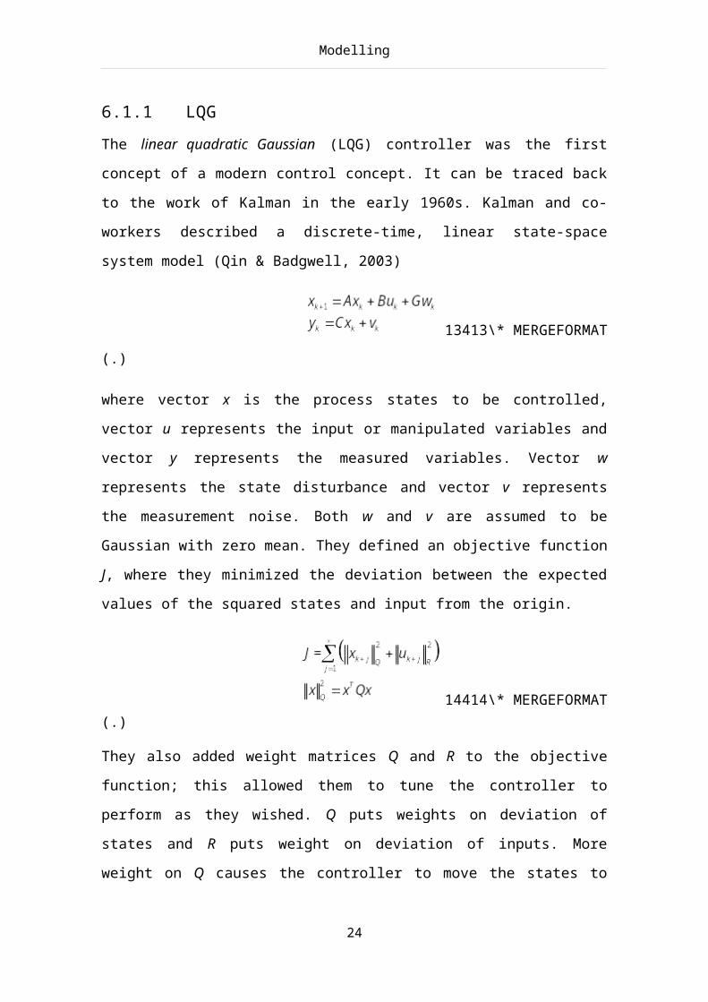
4.1.1 LQGThe linear quadratic Gaussian (LQG) controller was the first concept of a modern
control concept. It can be traced back to the work of Kalman in the early 1960s. Kalman
and co-workers described a discrete-time, linear state-space system model (Qin &
Badgwell, 2003)
13413\* MERGEFORMAT
(.)
where vector x is the process states to be controlled, vector u represents the input or
manipulated variables and vector y represents the measured variables. Vector w
represents the state disturbance and vector v represents the measurement noise. Both w
and v are assumed to be Gaussian with zero mean. They defined an objective function J,
where they minimized the deviation between the expected values of the squared states
and input from the origin.
14414\* MERGEFORMAT(.)
16

Introduction to Model Predictive Control
They also added weight matrices Q and R to the objective function; this allowed them to
tune the controller to perform as they wished. Q puts weights on deviation of states and
R puts weight on deviation of inputs. More weight on Q causes the controller to move
the states to its setpoint faster. Q has to be positive semi-definite and R has to be
positive definite to ensure that the objective function is convex. A convex optimization
problem always has a unique optimal solution, and can easily be solved using
commercial mathematical products like MATLAB.
The solution to this problem involves two steps; first the outputs measurement y at time
k is used to obtain an optimal state estimate
15415\*
MERGEFORMAT (.)
where Kf is the Kalman filter gain, and is computed from the solution of a matrix Ricatti
equation (Qin & Badgwell, 2003).
Second; an optimal input uk is computed using an optimal proportional state controller
. The LQG controller has good stabilizing properties; given that the linear
internal model is almost identical to the real plant. One big drawback for the LQG
controller is that it doesn’t handle constraints on inputs and states.
4.2 MODEL PREDICTIVE CONTROL
The major difference between today’s MPC technology and to ordinary LQG is that
MPC handles constraints on inputs, states and outputs. This is an important feature,
because a plant almost always have constraints on input and also often on states and
outputs.
There are several variants of the MPC, but they all share common trait that an explicitly
process model is used to predict and optimize future process behaviour (Hovd, 2009).
The following section presents some of the features that are common and important for
MPCs. The discussion given here will focus on linear MPC.
17

Introduction to Model Predictive Control
4.2.1 THE OBJECTIVE FUNCTION
The objective function in the MPC contains all the variables that are weighted, that are
all inputs and all outputs that are of interests, but it can also be states that indirectly
improve an output that can be difficult to measure correctly. The optimization problem
is typically cast into one of two standard forms (Hovd, 2009):
Linear programming (LP) formulation, where both the objective function and
constraints are linear.
Quadratic programming (QP) formulation, where the objective function is
quadratic and whereas the constraints have to be linear.
A quadratic objective function generally gives smoother control and more intuitive
tuning parameters (Hovd, 2009). In the LQR algorithm, the objective function given by
equation 414is defined over an infinite horizon and it takes into account infinite number
of steps into the future. This is only possible when there are no constraints in the
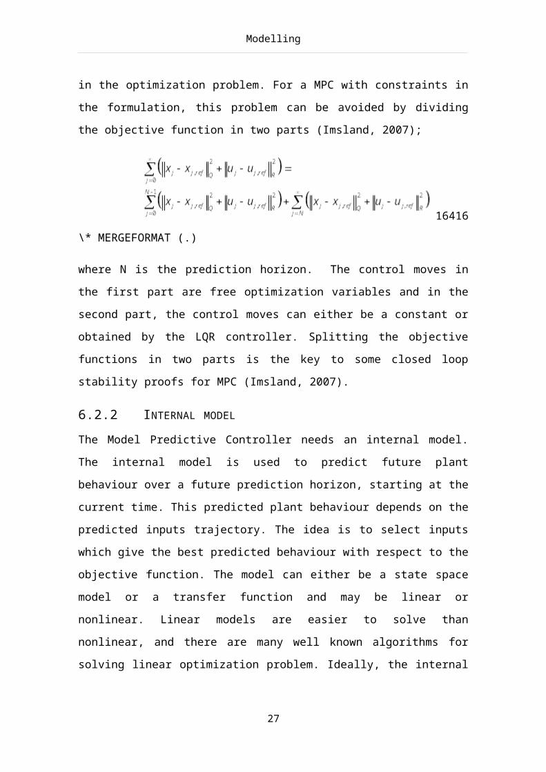
optimization problem. For a MPC with constraints in the formulation, this problem can
be avoided by dividing the objective function in two parts (Imsland, 2007);
16416\*
MERGEFORMAT (.)
where N is the prediction horizon. The control moves in the first part are free
optimization variables and in the second part, the control moves can either be a constant
or obtained by the LQR controller. Splitting the objective functions in two parts is the
key to some closed loop stability proofs for MPC (Imsland, 2007).
4.2.2 INTERNAL MODEL
The Model Predictive Controller needs an internal model. The internal model is used to
predict future plant behaviour over a future prediction horizon, starting at the current
time. This predicted plant behaviour depends on the predicted inputs trajectory. The
idea is to select inputs which give the best predicted behaviour with respect to the
objective function. The model can either be a state space model or a transfer function
18

Introduction to Model Predictive Control
and may be linear or nonlinear. Linear models are easier to solve than nonlinear, and
there are many well known algorithms for solving linear optimization problem. Ideally,
the internal model should behave similar to the real process in order to achieve good
control in practice. If the model does not exhibit similar characteristics to those of the
real plant, the MPC would have difficulties finding the optimal inputs to the process.
4.2.3 CONTROL INTERVAL
An MPC generates a discrete-time controller, which is a controller that takes action at
regular discrete time instants, in other words, applies new computed inputs to the plant.
This is often referred to as sampling time. The time that is separating each sampling
interval is often referred to as control interval. One would have a small control interval,
because the MPC could adjust faster for deviation in measured outputs. But too small a
control interval would also lead to failure, due to the fact that the MPC cannot finish the
computation in time. It can also be dangerous to set the control interval too large
because this might lead to bad closed loop performance. One can say that the control
interval should be at least as long as the computation time, but not so long that it will
affect the closed loop performance. With modern computer power, short control
intervals are usually not a large problem, as long as the optimization problem is linear
and there are not too many variables to optimize.
4.2.4 PREDICTION HORIZON
The prediction horizon is the time horizon which the controller predicts the future
outputs when computing controller moves. In addition to having an effect on closed
loop performance, the prediction horizon also affects the complexity of the
computation. One can usually say that a large prediction horizon gives larger
complexity and better closed loop performance, whereas a small prediction horizon
gives the opposite. From a control point of view, one can say that the prediction horizon
should be limited by computational bounds, but this might not always be a good choice.
One always has model mismatch, due to nonlinearities, simplifications and modelling
errors, and these uncertainties tend to be amplified as one predicts far into the future
(Imsland, 2007).
19

Introduction to Model Predictive Control
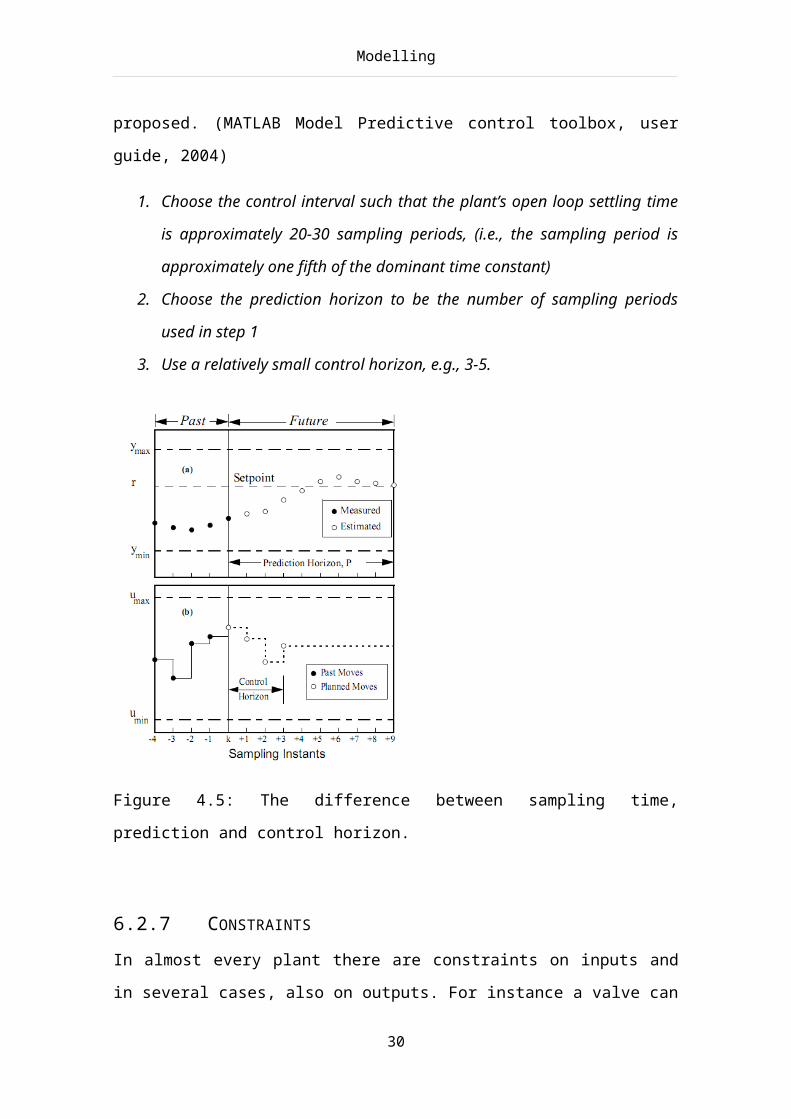
4.2.5 CONTROL HORIZON
The control horizon is the number of future optimal control moves computed at each
sampling time. At the next sampling time, a new optimal control input is computed.
Figure 4.5 shows the difference between control interval, and prediction and control
horizon (MATLAB Model Predictive control toolbox, user guide, 2004).
4.2.6 HOW TO CHOOSE GOOD INTERVAL AND HORIZONS
It can be difficult to choose correct values for control interval, prediction and control
horizon, but some rules of thumb for lag dominant, stable processes have been
proposed. (MATLAB Model Predictive control toolbox, user guide, 2004)
1. Choose the control interval such that the plant’s open loop settling time is
approximately 20-30 sampling periods, (i.e., the sampling period is
approximately one fifth of the dominant time constant)
2. Choose the prediction horizon to be the number of sampling periods used in step
1
3. Use a relatively small control horizon, e.g., 3-5.
20

Introduction to Model Predictive Control
Figure 4.5: The difference between sampling time, prediction and control horizon.
4.2.7 CONSTRAINTS
In almost every plant there are constraints on inputs and in several cases, also on
outputs. For instance a valve can never be more than fully open or it is desirable to keep
an output within a lower and upper bound. There are two kinds of constraints, hard
constraints and soft constraints. Hard constraints are constraints that cannot be violated
under any circumstances; the MPC will always try to satisfy hard constraints before any
other constraints or setpoints. It is most common to put hard constraints on input
variables, such as valves, pumps and so on, because this is equipment that has a physical
limit. It is also possible to put constraints on how much an input can move in each time
step. It can be risky to have hard constraints on an output, because the MPC will ignore
its other objectives in order to satisfy them, causing other outputs to be driven away
from their setpoint. Soft constraints are constraints that can be violated to satisfy other
constraints. The constraints can be written in the following form.
21
Introduction to Model Predictive Control
17417\*
MERGEFORMAT (.)
where u is the input vector, ∆u is the input change from one control sampling time to
the next, and y is the output vector. They can be written compactly (Imsland, 2007)
18418\* MERGEFORMAT (.)
where Dx and Dy are matrices that must be constructed, and are vectors of suitable
dimension, and u is the input vector and x is the output vector.
4.2.8 INFEASIBILITY
In some cases, the MPC encounters a situation where all the constraints cannot be
satisfied, this may happen when large disturbances affect the process. This situation is
called infeasibility and it is important that the MPC can handle such situations. One way
to cope with infeasibility is to temporarily remove the constraints, which are violated,
from the optimization and then add the constraints when the output returns to its
feasible area. Another alternative is to use soft constraints instead of hard constraints;
this will cause the MPC to try to satisfy all its objectives without removing constraints
that are violated.
4.2.9 MPC TUNING
As mentioned in chapter 4.1.1, it is possible to tune the controller with the matrices Q
and R. Different values of Q and R matrices will give different performances.
Consideration of the objective function given in equation 416 reveals that Q penalizes
deviation of states and outputs and R penalizes deviation between the optimal input and
their setpoint value. Increasing the weights on the R matrices relative to the weights on
Q will reduce the control activity and may even reduce the control activity to zero,
causing steady state error on states and outputs. Too large weights on R will also give
22

Introduction to Model Predictive Control
slow response to disturbances. Different values of the diagonal R matrix elements will
cause one input to move more than another input. Suppose that two inputs have an
almost identical influence on an output, then the MPC will use the input, which has the
lowest weight to bring the output to its setpoint. The same goes for the weights in the Q
matrix: The MPC will try to keep a state or output, which has a larger weight, at its
setpoint, prior to a state or output with lower weight. Other aspects that affect the tuning
are the disturbance model and the observer dynamics.
4.2.10 SQUARE PLANTS AND NON SQUARE PLANTS
In the real world, process inputs and outputs can be lost due to valve saturation,
hardware failure and so on, this means that the structure of the control problem and
degrees of freedom for control can change dynamically during operation. Figure 4.6
illustrates how the process can change. In the “thin” plant, there are not enough inputs
to meet all the control objectives and outputs may move freely. The control
specification needs to be relaxed or the output violation can be minimized in some mean
square sense (Qin & Badgwell, 2003). In the square plant, the amount of inputs is equal
to the amount outputs and the MPC is able to meet the control objectives. In the “fat”
case, which is more common, the plant has more inputs than outputs. The input values
needed to achieve a particular setpoint would be non unique, thus the inputs would drift
within their operating space. One way to avoid this is to use setpoints for extra inputs.
These setpoints are usually defined beforehand and may represent operational condition
that improves economical return, safety et cetera.
Figure 4.6: Process structure determines the degrees of freedom available to the controller. Adapted from Froisy (1994).
23

Introduction to Model Predictive Control
4.3 NONLINEAR MPCNonlinear Model Predictive Control is a variant of the linear model predictive control
(MPC). The difference between the nonlinear MPC and the linear MPC is that the
nonlinear MPC uses a nonlinear model to predict future plant behaviour. While for the
linear MPC, the optimization problem is convex, and it is therefore possible to
determine the computational time for each optimization step. The optimization problem
for nonlinear MPC is generally non-convex, which imposes challenges for both
numerical solution and stability. It is therefore hard, or impossible to determine the
computational time for each optimization step, and one can therefore not guaranty if the
optimization will complete in time. Since the optimization problem is non-convex, one
can in addition to the global optimal solution, which is the preferred solution, also have
many local optimal solutions. If the optimization algorithm converges to an optimal
solution, it is impossible to say if the solution found is a global optimal solution or not,
because the algorithm can as well converge to a local optimal solution.
In practice, linear MPC give good performance, so it often not worth to invest time and
money to implement a non-linear MPC, and due to the simple structure, linear MPC is
easier to maintain.
24

Process control theory
5 PROCESS CONTROL THEORY
1915Equation Chapter (Next) Section 1
In this chapter some theory for process control and heat exchangers are given.
5.1 CONTROL STRUCTURE
It is quite common to divide the control system into several layers, where each layer is
separated by a time scale. The layers are shown in Figure 5.7.
Figure 5.7: Control hierarchy (Skogestad, 2004).
where the supervisory control and regulatory control can be seen as the control layer.
The regulatory control layer often exists of single-input single-output PID control loops
that are used for stabilization and local disturbance rejection by controlling selected
“secondary” variables. The supervisory control layer consist of more advanced control
system, typically a MPC, and is used to keep primary outputs at their setpoint by
controlling setpoints for the regulatory control layer. The layers above can be seen as an
overall optimization layer that involves the whole plant and is controlled by an overall
real time optimizer (RTO).
The different layers also operate on different time scales. The top layer works on a
weekly or monthly basis, where the task is to schedule how the plant shall run the next
weeks or months. The site-wide optimization works on a daily, and the optimization
25
Process control theory
layer work on an hourly basis where a real time optimizer uses a model of the plant to
compute new optimal setpoints for supervisory level. This model is often a nonlinear
steady state model, which has to be maintained, so it matches the current plant
conditions. The supervisory level works on a smaller timescale, like minutes, while the
regulatory layer works on an even smaller timescale, seconds.
If an MPC is used at supervisory control layer, a regulatory layer is not required,
because the MPC is able to directly control physical inputs. However, since MPCs are
more complex and their sensitivity to errors and failure are quite unpredictable, such
controllers are usually avoided at the bottom control hierarchy (Skogestad, 2004).
Another alternative is to have the MPC at the supervisory layer control setpoints for
regulatory layer. This will ensure that the plant is running even if the MPC fails, thus
making the control system more failure tolerant.
The decentralized controllers should be tuned properly in order to obtain a good time
scale separation between the control layers. By doing this, there will be several
advantages according to Skogestad & Postlethwaite (2005):
The stability and performance of a lower (faster) layer is not much influenced by
the presence of upper (slow) layers because the frequency of the ”disturbance”
from the upper layer is well inside the bandwidth of the lower layer.
With the lower (faster) layer in place, the stability and performance of the upper
(slower) layers do not depend much on the specific controller settings used in
the lower layers because they only affect high frequencies outside the bandwidth
of the upper layers.
These items emphasize the importance of well tuned controllers in the lowest layer.
This thesis will focus on the lower layers in the control structure, and therefore the
higher layers will not be taken into consideration in this thesis.
26

Process control theory
(a) MPC controls setpoints for lower layer controllers.
(b) MPC controls directly on physical inputs.
Figure 5.8: Block diagram showing the two MPC alternatives.
5.2 CONTROL CHALLENGES OF HEAT EXCHANGERS
Heat exchanger networks (HEN) have been considered to be extremely nonlinear
(Shinskey, 1979). Both thermal effectiveness and heat transfer coefficients depend on
the flow rate through the heat exchanger, and this in the main cause for the
nonlinearities (Mathisen, 1994). In addition to the non-linearity, right half plane zeros
and time delays imposes fundamental limitations if control performance.
Plants with right half plane zeros may have inverse response and therefore fast
and efficient control are impossible with simple PID controllers. However with
the use of Model Predictive Control, the control performance can be improved
compared to simple PID controllers.
For HENs time delays are due to mass and energy holdup in heat exchangers and
mass holdup in pipes, and this also imposes a limitations of control performance
(Zeigler and Nichols, 1943; Rosenbrock, 1970). It is assumed that the time
delays at Brobekk are very small, because of fast flow rate through the pipes,
and is therefore neglected in the model.
The outlet temperatures from a heat exchanger can independently be controlled by
manipulating the inlet temperatures. But usually the inlet temperatures cannot be
27
Process control theory
manipulated, and one will therefore have to use the primary and secondary sides flow
rates to control the outlet temperatures. However, if the flow rate at one of the side of
the heat exchanger is fixed, i.e. not a manipulated variable, it is impossible to control
both outlet temperatures independently, i.e. one can only control one of the outlet
temperatures.
28
Implementation of MPC and simulations
6 IMPLEMENTATION OF MPC AND SIMULATIONS
2016Equation Chapter (Next) Section 1As mentioned in the problem description, one of the
tasks was to investigate whether it would be worthwhile to apply either an MPC or a
Nonlinear MPC for controlling the real plant. Considering the discussion in chapter 5.2
regarding nonlinearities of heat exchangers, a nonlinear MPC would theoretically be
preferred for controlling the real plant; however, due to the practical difficulties
regarding nonlinear MPCs discussed in chapter 4.3 we propose not to use a nonlinear
MPC. However, with the use of linear MPC for controlling the plant, an alternative is to
have several MPCs for different operating points and then switch between them to
account for non-linear behaviour.
However, in this thesis, it was decided to use MATLAB’s Model Predictive Control
Toolbox, which is a linear MPC. The main reasons for this are:
The model developed by Smedsrud is made in Simulink, which is a
supplementary package to MATLAB.
The Model Predictive Control Toolbox provides Simulink blocks and MATLAB
functions for designing and simulating model predictive controllers both in
MATLAB and Simulink. It is therefore easy to connect the model with a model
predictive controller.
The dynamic heat exchanger model derived in 3.1 uses linear differential
equations. It would not make any sense to use a nonlinear MPC.
MATLAB is in use in the in industry and can be used directly or linked with
other software packages.
The rest of this chapter presents the different MPCs alternatives that were designed for
the model of Brobekk waste incineration plant, and hopefully the results can be valuable
in order to solve the problems described in chapter 2.2
First, some theory on how the Model Predictive Toolbox works is presented. Secondly,
control challenges discovered at Brobekk are described. Lastly, simulation results are
present.
29

Implementation of MPC and simulations
30

Implementation of MPC and simulations
6.1 MATLAB MPC TOOLBOX
This section contains a little discussion of the Model Predictive Control Toolbox, but
the toolbox is described in greater detail in the MathWorks tutorial, Model Predictive
Control Toolbox, user guide, v2, 2004.
6.1.1 OPTIMIZATION PROBLEM
The optimization problem to be minimized is written:
21
621\* MERGEFORMAT (.)
Subject to
22622\*MERGEFORMAT (.)
where the subscript j denotes the j-th component of a vector, k+i|k denotes the value
predicted for time k+i based on the information available at time k; r is the reference for
all measured and unmeasured outputs, p is the prediction horizon, m is the control
horizon and ny and nu are the dimension of the input vector and output vector.
The optimization problem minimizes the objective function using information from the
present time step k to m−1+k and the slack variable ε as optimization variables. In
31
Implementation of MPC and simulations
equation 621, constraints are relaxed by introducing the slack variable ε ≥ 0. The weight
ρε on the slack variable ε penalize the violation of the constraints. The larger weight
with respect to manipulated variable and measured output weights, the more the
constraint violation is penalized (Model Predictive Control Toolbox, user guide, v2,
2004).
6.1.2 PREDICTION MODEL
MPC toolbox uses a linear model for prediction and optimization, and the idea is shown
in Figure 6.9.
Figure 6.9: Linear model for prediction and optimization.
The model consists of
A linear model of the plant to be controlled
A model for generating unmeasured disturbances
The linear time invariant system can be described by the equation:
23623\*
MERGEFORMAT (.)
Where x(k) is the state vector, u(k) is the manipulated variables, v(k) is the measured
disturbance vector, d(k) is the unmeasured disturbance vector, ym(k) is the measured
outputs and yu(k) is the unmeasured outputs. The overall output vector y(k) collects ym(k)
and yu(k).
32

Implementation of MPC and simulations
If an unmeasured disturbance model is not specified, the toolbox will generate one,
assuming that the disturbances are integrated white noise. The unmeasured disturbance
model is also modelled as a linear time invariant system.
24624\*
MERGEFORMAT (.)
Where nd is random Gaussian noise which have zero mean and unit covariance matrix.
6.2 CONTROL CHALLENGES AT BROBEKK PLANT
Brobekk waste incineration plant is a quite challenging plant to control, as Hafslund can
try to take out more than 32 MW or they may want to take out less than 32 MW. It is
therefore possible to split the control into two regions, one when Hafslund try to takes
out more than 32 MW, which is called α (alpha), and another, which is when Hafslund
takes out less than 32 MW, which is called β (beta). The heat demand q from Hafslund
can simply be found by using the steady state energy balance for heat exchangers
below.
25625\* MERGEFORMAT (.)
Where cp is the specific heat capacity, w is flow rate. Tout and Tin represents outlet and
inlet temperatures, and q is heat exchanged. Consideration of equation 625, reveals that
Tout depends on the flow rate w, the specific heat capacity cp, heat demand q, and
secondary side inlet temperature Tin. The maximum outlet temperature, Tout can
therefore be plotted as a function of flow rates at various inlet temperatures from Oslo.
If the desired temperature that Hafslund wants towards Oslo is above the maximum
outlet temperature, Hafslund wants to take out more than 32 MW and vice versa. All
curves are calculated based on q = 32 MW. The maximum outlet temperatures are
shown in Figure 6.10.
33

Implementation of MPC and simulations
500 550 600 650 700 750 800 850 90075
80
85
90
95
100
105
110
Flow rate [tonne/h]
Max
sim
um te
mpe
ratu
re to
Osl
o [o C
]
Tin=70
Tin=80
Tin=90
Figure 6.10: Maximum outlet temperature, Tout as a function of flow rate.
6.2.1 ALPHA REGION
The α region, defined as when Hafslund wants 32MW or more, is simple to control.
Since EGE never can achieve the desired temperature that Hafslund wants, the only
control objective is the furnace inlet temperature, y1.
6.2.2 BETA REGION
The β region, defined as when Hafslund wants less than 32MW, is more challenging; in
addition to controlling the furnace inlet temperature, the heat exchanger secondary side
outlet temperature, y10, should also be controlled. In this region, EGE has to use the air
coolers to remove the excess energy. A result of learning how the process works, it was
found that β region should be divided into 4 different sub regions, based on the
following factors
Furnace inlet temperature.
The heat exchanger primary side outlet temperature.
The air cooler primary side outlet temperature.
We will first explain the characteristics of each sub region, and why different sub
regions imposes control difficulties when using MPCs. At last we will explain why
34

Implementation of MPC and simulations
some of these sub regions can be undesirable to operate in. Figure 6.11 shows an
overview over the different sub regions.
Sub region 1The first sub region is when both the air cooler primary side outlet temperature, y6, and
the heat exchanger primary side outlet temperature, y8, are lower than the furnace inlet
temperature, y1. The only way that EGE can keep the furnace inlet temperature at it
setpoint, is to use the bypass valve.
The air cooler primary side outlet temperature is low due to cold air cooling the water
inside the air cooler when the air cooler is not used, and therefore the plant will always
be in this sub region when going from the α region the β region. As the air cooler valve
opens further, hot water will flow through the air cooler, and at one point, the air cooler
primary side outlet temperature, y6, will become higher than the furnace inlet
temperature. This brings the plant to the second sub region.
Sub region 2This sub region is described by the air cooler primary side outlet temperature, y6, is
higher than the furnace inlet temperature, y1, and the heat exchanger primary side outlet
temperature, y8 is lower than the furnace inlet temperature, y1.
Sub region 3In the third sub region the air cooler primary side outlet temperature, y6, is lower than
the furnace inlet temperature, y1 and the heat exchanger primary side outlet temperature,
y8, is higher than furnace inlet temperature, y1.
In this sub region and in sub region 2, EGE can keep the furnace inlet temperature at its
setpoint with the flow from the air cooler and heat exchanger, without using the bypass
valve.
Sub region 4The fourth sub region when both air cooler primary side outlet temperature, y6 and the
heat exchanger primary side outlet temperature, y8 are higher than the furnace inlet
temperature, y1. However, this region has not been considered in this thesis, because this
sub region is not permitted to operate in. There are no ways that EGE can keep the
furnace inlet temperature at its setpoint when operating in this sub region.
35

Implementation of MPC and simulations
Figure 6.11: The different sub regions at Brobekk.
Control difficultiesFrom an operational point of view, the temperatures within Brobekk should be able to
change freely as long the furnace inlet temperature and heat exchanger secondary side
outlet temperature follows its setpoints. The problem is that the gains from the air cooler
valve and heat exchanger valve to the furnace inlet temperature will change sign when
the plant is in operation. For instance, this happens when the plant switches from sub
region 1 to sub region 2. This is shown in Figure 6.11 and Figure 6.12.
As mentioned in chapter 4.2.2 the MPC uses an internal model to predict future plant
behaviour. When the plant drastically changes characteristics, the MPC will fail to find
an optimal input, because the internal model does not exhibit the similar characteristics
as the real plant. One alternative to avoid that gains change, is to control the primary
36

Implementation of MPC and simulations
side outlet temperatures at the air cooler and heat exchanger when EGE operates in the
in the β region. Another alternative is to have different MPCs for each sub region where
each MPC has a proper internal model and then change between them when needed.
50 100 150 200
0
Furnace inlet temperature [oC]
Neg
ativ
e ga
in
P
ositi
ve g
ain
Figure 6.12: Example how the gain changes when the plant is in operation.
Undesirable region
Considering the sub region 1, it can be revealed that this is an undesirable sub region to
operate in. The problem with this sub region is that both the air cooler primary side and
heat exchanger primary side outlet temperatures are lower than the furnace inlet
temperature, thus EGE has to use the bypass valve to keep the furnace inlet temperature
at its setpoint. When the bypass valve opens, less water will flow through the heat
exchanger and air cooler, thus the heat exchanger and air cooler primary side outlet
temperatures will decrease even more. If EGE has to remove more excess heat in the air
cooler, the air cooler fan will blow more air though the secondary side of the air cooler,
lowering the air cooler primary side outlet temperature. The bypass valve will opens
more in order to keep the furnace inlet temperature at its setpoint. This approach works
to a situation where the bypass valve is fully open but when the bypass valve saturates
EGE will lose control over the furnace inlet temperature. The above discussion
emphasize that this sub region is undesirable, and thus EGE should try to avoid
operating in it. Instead they will have to force the plant into sub region 2 or 3.
Unfortunately the plant will always be in sub region 1, when switching from the α
region to the β region, which is explained in the section “sub region 1” on page 34.
37

Implementation of MPC and simulations
Thus EGE cannot avoid to operate in it when switching from the α to the β region, but
they can make some logic that will force the plant into sub region 2 or 3.
Transition between α and β region
When switching from the α region to the β region, it will make most sense to force the
process into sub region 2, because the heat exchanger primary side outlet temperature
already is lower than the furnace inlet temperature. The heat exchanger primary side
outlet temperature is lower than the furnace inlet temperature due to the use of the
bypass valve when EGE operates in the α region. This can be proved by considering the
following equation.
26626\* MERGEFORMAT (.)
Where cp is the specific heat capacity, w is flow rate. Tout and Tin represents outlet and
inlet temperatures, and q is conducted heat. If the total heat q is 16 MW, the inlet
temperature is 180°C, and the flow through the heat exchanger is 250 tonne/h, this will
give an outlet temperature at 126°C. But if the flow through the heat exchanger
decreases, the heat exchanger outlet temperature will also decrease, and thus become
lower than the furnace inlet temperature. The flow through the heat exchanger will
decrease below 250 tonne/h when the bypass valve is used, which always is the case
when operating in the α region and in sub region 1
The transition from the α region to the β region requires special care. The transition can
be compared to driving a car and keeping a constant speed while pushing the brakes.
The driver has to use the accelerator to maintain the speed. To make it even more
difficult, the brake will at some point change to an accelerator.
SummaryThe above discussion regarding the different regions can be summarized to
There is no problem when operating in the α region.
When switching from the α region to the β region, the plant must be forced in to
sub region 2, which a is the recommended sub region to operate in.
38

Implementation of MPC and simulations
When operating in sub region 2, the bypass valve should be closed all times, to
prevent to plant to enter sub region 1.
Figure 6.13 shows how the plant should operate when switching between different
regions.
Figure 6.13: Transition between different regions.
6.3 CONTROL STRUCTURE DESIGN
In order for the model predictive controller to be as simple as possible, some control
loops, in particular frost protection, air heater and main flow controller, were excluded
from the MPC design. These control loops are not heavily affected by disturbances form
Hafslund. PI controllers were therefore designed for these control loops.
The MPCs had therefore a total of four manipulated variables, the bypass valve, the heat
exchanger valve, and the air cooler fan and valve. Since it is assumed that the two heat
exchanger lines are almost identical, an MPC developed for heat exchanger line 1 also
will work for line 2, and since EGE do not control any valves at Hafslund side of the
heat exchanger, EGE do not violates Hafslund’s control structure.
It was decided to let the MPC control directly on manipulated inputs, and reasons for
this are
The main flow at Brobekk is already controlled.
The flow in through the bypass or the primary side of the heat exchanger is not
measured.
However, when the plant is in the β region, one alternative for controlling the heat
exchanger secondary side outlet temperature could be to let the MPC calculate a
39

Implementation of MPC and simulations
setpoint for the heat exchanger primary side flow. A flow controller could then control
this flow. The rest of the flow in the plant would then go through the air cooler, which
needs to be left uncontrolled. But this is not possible because obvious reason above.
6.3.1 PI CONTROLLERS
Steady state gain k and time constant τ1 were obtained by using step responses and then
approximation of a first-order transfer function model. The tuning parameters for PI
controllers were then found using Skogestad/Simple Internal Model Control (SIMC)
(Skogestad, 2003).
The controller gain and integral action are given by.
27627\* MERGEFORMAT (.)
28628\* MERGEFORMAT
(.)
Table 6.5: PI Controller parameters.
Controller k τ1 θ τc Kc τi
Air heater 90 100 1 1 0.55 8Air cooler – frost protection 4800 2423 10
0100 0.0025 800
Brobekk flow controller1 5.342 ∗10-
3
9.43 ≪1
≪1
37 0.2
It was decided to set the tuning parameter τc equal to θ. This gives a reasonably fast
response with moderate input usage and good robustness margins (Skogestad, 2003).
The controllers were modelled using a standard PI controller equation 629. The open
loops responses are shown in appendix C.
1 The controller parameters for the main flow controller had to be retuned because SIMC gave a too high controller gain.
40

Implementation of MPC and simulations
29629\* MERGEFORMAT (.)
Figure 6.14 (a) shows the air temperature toward the furnace follows its setpoint at
90°C. The flow through the air heater secondary side was set to 6 kg/s. Figure 6.14 (b)
shows the disturbances that affect the air temperature towards the furnace, which is the
primary side inlet temperature and primary side flow. The outside air temperature was
set to 0°C.
Figure 6.15 (a) shows that frost protection controls the temperature trajectory inside the
air cooler. At time 8000 sec the temperature controller in frost protection system starts
to stabilize temperature at 10°C. Figure 6.15 (b) shows the flow through the air cooler
valve, which is used to stabilize the temperature inside the air cooler. Figure 6.15 (c)
shows the flow inside the air cooler, which always is 15.125 kg/s, and the flow driven
by the frost protection pump, which depends on the flow through the air cooler valve.
The outside air temperature was set to 0°C.
Figure 6.16 shows the flow towards the furnace. The setpoint for this flow is 250
tonne/h, which is in accordance with the operational aspect at Brobekk.
0 0.2 0.4 0.6 0.8 1 1.2 1.4 1.6 1.8 2
x 104
89.96
89.98
90
90.02
90.04Air temperature towards furnace
Time [s]
[o C]
0 0.2 0.4 0.6 0.8 1 1.2 1.4 1.6 1.8 2
x 104
179.5
180
180.5
181Inlet temperature - Air heater primary side
Time [s]
[o C]
0 0.2 0.4 0.6 0.8 1 1.2 1.4 1.6 1.8 2
x 104
3.6
3.8
4
4.2Flow Hotside out
Time [s]
[kg/
s]
(a)
41

Implementation of MPC and simulations
0 0.2 0.4 0.6 0.8 1 1.2 1.4 1.6 1.8 2
x 104
89.96
89.98
90
90.02
90.04Outlet temperature - Air heater secondary side
Time [s]
[o C]
0 0.2 0.4 0.6 0.8 1 1.2 1.4 1.6 1.8 2
x 104
179.5
180
180.5
181Inlet temperature - Air heater primary side
Time [s]
[o C]
0 0.2 0.4 0.6 0.8 1 1.2 1.4 1.6 1.8 2
x 104
3.6
3.8
4
4.2Flow Hotside out
Time [s]
[kg/
s]
(b)
Figure 6.14: Air temperature towards the furnace and disturbances.
0 0.2 0.4 0.6 0.8 1 1.2 1.4 1.6 1.8 2
x 104
0
50
100
150
200Outlet temperature - Air cooler primary side
Time [s]
[o C]
0 0.2 0.4 0.6 0.8 1 1.2 1.4 1.6 1.8 2
x 104
-0.05
0
0.05
0.1
0.15Flow trough the air cooler valve
Time [s]
[kg/
s]
0 0.2 0.4 0.6 0.8 1 1.2 1.4 1.6 1.8 2
x 104
15.1
15.15
15.2
15.25
15.3Flow trough the pump and air cooler
Time [s]
[kg/
s]
Flow through the pumpFlow through the air cooler
(a)0 0.2 0.4 0.6 0.8 1 1.2 1.4 1.6 1.8 2
x 104
0
50
100
150
200Outlet temperature - Air cooler primary side
Time [s]
[o C]
0 0.2 0.4 0.6 0.8 1 1.2 1.4 1.6 1.8 2
x 104
-0.05
0
0.05
0.1
0.15Flow trough the air cooler valve
Time [s]
[kg/
s]
0 0.2 0.4 0.6 0.8 1 1.2 1.4 1.6 1.8 2
x 104
15.1
15.15
15.2
15.25
15.3Flow trough the pump and air cooler
Time [s]
[kg/
s]
Flow through the pumpFlow through the air cooler
(b)
42
Implementation of MPC and simulations
0 0.2 0.4 0.6 0.8 1 1.2 1.4 1.6 1.8 2
x 104
0
50
100
150
200Outlet temperature - Air cooler primary side
Time [s]
[o C]
0 0.2 0.4 0.6 0.8 1 1.2 1.4 1.6 1.8 2
x 104
-0.05
0
0.05
0.1
0.15Flow trough the air cooler valve
Time [s]
[kg/
s]
0 0.2 0.4 0.6 0.8 1 1.2 1.4 1.6 1.8 2
x 104
15.1
15.15
15.2
15.25
15.3Flow trough the pump and air cooler
Time [s]
[kg/
s]
Flow through the pumpFlow through the air cooler
(c)
Figure 6.15: Temperature and flow inside air cooler.
0 0.2 0.4 0.6 0.8 1 1.2 1.4 1.6 1.8 2
x 104
248
249
250
251
252Flow to Furnace [Tonne/h]
Time [s]
[Ton
ne/h
]
Figure 6.16: Main flow at Brobekk.
6.3.2 MPC DESIGN - ALPHA REGION
In the α region, EGE can never achieve the heat exchanger secondary side outlet
temperature, y10 , that Hafslund wants, will therefore not make sense to control this
variable. Thus EGE only has one variable to control, namely the furnace inlet
temperature, y1. Because EGE do not want to remove some heat in this region, they
have to close the air cooler valve, u7 and air cooler fan, u3. EGE now has two
manipulated variables left, the bypass valve u7 and heat exchanger valve u6 and one
controlled variable, making this a “fat” plant. As mentioned in chapter 4.2.10 that in the
“fat” plant case one need setpoint for extra manipulated variables, usually to improve
economical return or safety. From an economical point of view, EGE will have as much
water as possible through the heat exchanger, thus having the heat exchanger valve fully
43

Implementation of MPC and simulations
open at all time. If the heat exchanger valve is fully open, EGE only has one
manipulated variable and one control variable which is an optimal solution.
6.3.3 MPC DESIGN - BETA REGION
As mentioned earlier, the β region is quite challenging to control, first of all because of
the gains changes, and also because both the air cooler valve and the air cooler fan are
dependent on each other. The air cooler fan will not affect furnace inlet temperature if
the air cooler valve does not open, and the air cooler valve will operate at as hot bypass
if the fan does not start.
As discussed in chapter 6.2.2 the bypass valve has to be closed when EGE operates in
the β region, and in chapter 5.2 it was discovered that it is only possible to control one
outlet temperature, if one of the flows through the heat exchanger and both the inlet
temperatures are fixed, i.e. not possible to manipulate them. Since both the inlet
temperatures and the flow through the secondary side at the heat exchanger are fixed
and EGE controls the heat exchanger secondary side outlet temperature, it is not
possible to control the heat exchanger primary side outlet temperature independently.
The same goes for the air heater, because both the inlet temperatures and flow through
the secondary side are fixed, and EGE controls the secondary side outlet temperature.
This means that EGE only can control the furnace inlet temperature with the flow from
the air cooler and fan duty, because it is not possible to control the air heater and heat
exchanger primary side outlet temperature independently. Therefore three different
MPCs has to be developed for the β region, one for each sub region, except from sub
region 4.
6.4 SIMULATIONS
This section shows simulations of different MPC alternatives for both α and β region.
MPC parameters are shown in Table 6.6 through Table 6.8.
The internal models needed for the MPC were found using linear analysis in Simulink.
The basic model was the Simulink model developed by Smedsrud in his master thesis
and modified in this thesis. Appropriate manipulated and measured variables were
44

Implementation of MPC and simulations
chosen and then different internal models could be obtained by doing a linear analysis
of the basic model with steady state values. The internal model derived from the linear
analysis above had between 90-80 states; it was therefore decided to do a model
reduction of the model. Since the internal models are linear, a model reduction can
easily be done in MATLAB. The appropriate reduced model order should be greater or
equal to the number of dominant singular Hankel values. It was found that the
appropriate model order should be 20. After the model reductions were done, different
MPCs could be developed and implemented. All the simulations were done in Simulink.
Some of the parameters shown below are tuning parameters; according to Maciejowski,
(2002) tuning parameters are weighting matrices, prediction horizon, and observer and
disturbance model dynamics. A specific disturbance model was not included, so the
Model Predictive Control toolbox had to generate one.
Large weights on measured outputs were needed to ensure good control, large weights
on manipulated variables rate of change were needed to ensure smother response and
large weights were needed on manipulated variables to prevent them from moving. The
control interval, prediction and control horizon was determined based on the tuning
rules proposed in chapter 4.2.6.
6.4.1 ALPHA REGION
Only one control structure was considered for the α region. Large weights were put on
heat exchanger valve, and air cooler fan and valve, to prevent these manipulated
variables to move away from its setpoint. The setpoint was set is set to one for the heat
exchanger valve and zero for the air cooler fan and valve. The bypass valve is not
weighted at all, meaning that it can move freely within its operating space. The only
weighted output is the furnace inlet temperature and the setpoint was 126°C. The MPC
parameters are shown in Table 6.6.
45

Implementation of MPC and simulations
Table 6.6: Parameters for MPC constructed for α region.
Internal ModelOrder 20Manipulated variable u=[u8 u6 u3 u7]T
Measured variables y=[y12 y7 y1 y10 y8]T
Measured disturbances d=[d1 d2]T
Tuning parametersControl interval 30Prediction horizon 20Control horizon 3Manipulated variable setpoints [1 0.4 0 0]T
Manipulated variable weighting diag(Ru) = [10000 0 1000000 1000000]Manipulated variable rate of change weighting
diag(R∆u) = [1000 10000 1000000 1000000]
Measured outputs weighting diag(Qy)= [0 0 10000 0 0]Constraints specificationsMinimum MV umin = [0.55 0 0 0]T
Maximum MV umax = [1 1 90000 1]T
Minimum rate of change MV ∆umin = -[0.02 0.05 5000 0.02]T
Maximum rate of change MV ∆umax = [0.02 0.05 5000 0.02]T
No specific constraints were defined for measured outputs and no additional tuning was
done for the observer and the disturbance model, meaning that the default settings were
used.
Figure 6.17 (a) shows that the furnace inlet temperature follows its setpoint excellently.
The maximum deviation is approximately 0.5°C, which is within the measurement
accuracy. Figure 6.17 (b) shows how the heat exchanger secondary side outlet
temperature varies. And it can be seen that the heat exchanger outlet temperature never
reaches the temperature that Hafslund wants. Temperature, flow and heat demand from
Hafslund are shown in Figure 6.19. The heat demand is found by using equation 625.
Figure 6.18 shows how the manipulated variables vary during the simulation. The heat
exchanger valve is almost fully open at all time while the bypass valve is used to control
the furnace inlet temperature. The small drops in the heat exchanger valve are because
the valve is not enough heavily weighted compared to the other variables. But the drops
are less than 5% of the maximum valve opening, so it is believed that these drops do not
affect the control much. Most of the time, the valve is fully open. Plots of air cooler fan
and valve are not shown because they are not used in the α region.
46

Implementation of MPC and simulations
0 0.2 0.4 0.6 0.8 1 1.2 1.4 1.6 1.8 2
x 104
124
125
126
127
128Furnace inlet temperature
Time [s]
[o C]
0 0.2 0.4 0.6 0.8 1 1.2 1.4 1.6 1.8 2
x 104
90
100
110
120
130Outlet temperature - Heat exchanger secondary side
Time [s]
[o C]
Outlet temperatureSetpoint from Hafslund
(a) 0 0.2 0.4 0.6 0.8 1 1.2 1.4 1.6 1.8 2
x 104
125
125.5
126
126.5
127Furnace inlet temperature
Time [s]
[o C]
0 0.2 0.4 0.6 0.8 1 1.2 1.4 1.6 1.8 2
x 104
90
95
100
105
110
115Outlet temperature - Heat exchanger secondary side
Time [s]
[o C]
Outlet temperatureSetpoint from Hafslund
(b)
Figure 6.17: Figure (a) shows furnace inlet temperature and figure (b) shows the heat exchanger secondary side outlet temperature in the α region.
47

Implementation of MPC and simulations
0 0.2 0.4 0.6 0.8 1 1.2 1.4 1.6 1.8 2
x 104
0.9
0.95
1Heat exchanger valve
Time [s]
Val
ve o
peni
ng [0
-1]
0 0.2 0.4 0.6 0.8 1 1.2 1.4 1.6 1.8 2
x 104
0.4
0.6
0.8
1Bypass valve valve
Time [s]
Val
ve o
peni
ng [0
-1]
0 0.2 0.4 0.6 0.8 1 1.2 1.4 1.6 1.8 2
x 104
-1
-0.5
0
0.5
1Air cooler fan
Time [s]
[W]
0 0.2 0.4 0.6 0.8 1 1.2 1.4 1.6 1.8 2
x 104
-1
-0.5
0
0.5
1Air cooler valve
Time [s]
Val
ve o
peni
ng [0
-1]
Figure 6.18: Manipulated variables in the α region.
0 0.2 0.4 0.6 0.8 1 1.2 1.4 1.6 1.8 2
x 104
60
65
70
75Temperature from Hafslund
Time [s]
[o C]
0 0.2 0.4 0.6 0.8 1 1.2 1.4 1.6 1.8 2
x 104
700
800
900
1000Flow from Hafslund
Time [s]
[Ton
ne/h
]
0 0.2 0.4 0.6 0.8 1 1.2 1.4 1.6 1.8 2
x 104
30
35
40
45Heat demand from Hafslund
Time [s]
[MW
]
Figure 6.19: Flow, temperature and heat demand from Hafslund in the α region.
48

Implementation of MPC and simulations
6.4.2 BETA REGIONTwo control structures developed for the β region is shown in this thesis. They are
almost identical, but the difference between the two alternatives is the setpoint for the
heat exchanger secondary side outlet temperature. Several other control structures were
also tested, including the one where the Brobekk bypass valve was used, but none of
them seemed to give promising results, and there are therefore not shown here.
Alternative 1
In alternative 1, there are three manipulated variables, the heat exchanger valve, u8 and
air cooler fan u3 and valve u7, and two control variables, the furnace inlet temperature, y1
and heat exchanger secondary side outlet temperature, y10. The setpoint for the furnace
inlet temperature was 126°C and the setpoint for the heat exchanger secondary side
outlet temperature was equal to the setpoint for the temperature towards Oslo, y11.
Therefore Hafslund do not has to use their bypass valve to control the temperature
towards Oslo, and this bypass valve should be closed all the time.
Table 6.7: Parameters for MPC constructed for β region2.
Internal ModelOrder 20Manipulated variable u=[u8 u6 u3 u7]T
Measured variables y=[y12 y7 y1 y10 y8]T
Measured disturbances d=[d1 d2]T
Tuning parametersControl interval 30Prediction horizon 20Control horizon 3Manipulated variable setpoints uTarget = [1 0 5000 0.5]T
Manipulated variable weighting diag(Ru) = [100 500000 0 50]Manipulated variable rate of change weighting diag(R∆u) = [100000 10000 10 10000]Measured variables weighting diag(Qy)= [0 0 10000 7500 0]Constraints specificationsMinimum MV umin = [0 0 0 0]T
Maximum MV umax = [1 1 90000 1]T
Minimum rate of change MV ∆umin = -[0.02 0.05 5000 0.02]T
Maximum rate of change MV ∆umax = [0.02 0.05 5000 0.02]T
No specific constraints were defined for measured outputs and no additional tuning was
done for the observer and the disturbance model, meaning that the default settings were
2 The MPC parameters given in Table 6.7 are only valid for sub region 2 and 3. MPC parameters for sub region 1 are given in Table 6.8.
49

Implementation of MPC and simulations
used. As seen from Table 6.7, large weight was put on the bypass valve to prevent it
from move away from it setpoint, which was set to zero, and small weights were put on
the heat exchanger valve, and air cooler fan and valve so they could move freely. In
addition to having large weight on the furnace inlet temperature, large weight was put
on the heat exchanger secondary side outlet temperature.
Figure 6.20 (a) shows furnace inlet temperature. The deviation is slightly larger than for
the α region, 1.5°C against 0.5°C, but overall the control is good. At time step 6000
Hafslund changes the setpoint for the temperature towards Oslo and the controller needs
some time to bring the furnace inlet temperature back to its setpoint. Figure 6.22 shows
the inlet temperature, flow and heat demand from Hafslund. As seen from Figure 6.20
(b), the heat exchanger secondary side outlet temperature follows its setpoint well. The
maximum deviation is less than 1°C. The bypass valve at Hafslund was closed during
simulation, so the temperature shown in Figure 6.20 (b) will be the temperature towards
Oslo. Figure 6.21 shows how the manipulated variables vary during simulation. The
bypass valve at Brobekk is closed during the whole simulation while the manipulated
variables varies.
50

Implementation of MPC and simulations
0 0.2 0.4 0.6 0.8 1 1.2 1.4 1.6 1.8 2
x 104
124
125
126
127
128Furnace inlet temperature
Time [s]
[o C]
0 0.2 0.4 0.6 0.8 1 1.2 1.4 1.6 1.8 2
x 104
100
105
110
115
120
125Outlet temperature - Heat exchanger secondary side
Time [s]
[o C]
Outlet temperatureSetpoint from Hafslund
(a) 0 0.2 0.4 0.6 0.8 1 1.2 1.4 1.6 1.8 2
x 104
125
125.5
126
126.5
127Furnace inlet temperature
Time [s]
[o C]
0 0.2 0.4 0.6 0.8 1 1.2 1.4 1.6 1.8 2
x 104
104
106
108
110
112Outlet temperature - Heat exchanger secondary side
Time [s]
[o C]
Outlet temperatureSetpoint from Hafslund
(b)
Figure 6.20: Figure (a) shows furnace inlet temperature and figure (b) shows the heat exchanger secondary side outlet temperature in the β region alternative 1.
51

Implementation of MPC and simulations
0 0.2 0.4 0.6 0.8 1 1.2 1.4 1.6 1.8 2
x 104
0.4
0.6
0.8
1Heat exchanger valve
Time [s]
Val
ve o
peni
ng [0
-1]
0 0.2 0.4 0.6 0.8 1 1.2 1.4 1.6 1.8 2
x 104
-5
0
5
10
15x 10
-3 Bypass valve valve
Time [s]
Val
ve o
peni
ng [0
-1]
0 0.2 0.4 0.6 0.8 1 1.2 1.4 1.6 1.8 2
x 104
1
2
3
4
5x 10
4 Air cooler fan
Time [s]
[W]
0 0.2 0.4 0.6 0.8 1 1.2 1.4 1.6 1.8 2
x 104
0.4
0.6
0.8
1Air cooler valve
Time [s]
Val
ve o
peni
ng [0
-1]
Figure 6.21: Manipulated variables in the β region alternative 1
52

Implementation of MPC and simulations
0 0.2 0.4 0.6 0.8 1 1.2 1.4 1.6 1.8 2
x 104
82
84
86
88Temperature from Hafslund
Time [s]
[o C]
0 0.2 0.4 0.6 0.8 1 1.2 1.4 1.6 1.8 2
x 104
700
800
900
Flow from Hafslund
Time [s]
[Ton
ne/h
]
0 0.2 0.4 0.6 0.8 1 1.2 1.4 1.6 1.8 2
x 104
15
20
25
30Heat demand from Hafslund
Time [s]
[MW
]
Figure 6.22: Flow, temperature and heat demand from Hafslund in the β region.
Alternative 2
In alternative 2, the heat exchanger secondary side outlet temperature setpoint was 2°C
higher than the setpoint for the temperature towards Oslo, thus Hafslund uses their
bypass valve to control the temperature towards Oslo. The MPC developed for
alternative 1 was used in alternative 2, as well as the same temperature and flow from
Hafslund. Figure 6.23 (a) shows that the furnace inlet temperature varies a lot more than
in alternative 1, but the deviations in temperature never exceeds ±2°C. The heat
exchanger secondary side outlet temperature varies even more and the deviations is
somewhere about 7°C. Figure 6.25 shows the flow through the heat exchanger
secondary side. The flow varies a lot and this again affects the furnace inlet temperature
and the heat exchanger primary side outlet temperature. This variation in flow is caused
by the bypass valve at Hafslund side, if the valve opens, less water will flow through the
heat exchanger and vice versa. Figure 6.24 shows the temperature towards Oslo and it
53
Implementation of MPC and simulations
follows the setpoint exceptionally good on the expense of more variations in
temperature at Brobekk’s side of the heat exchanger.
0 0.2 0.4 0.6 0.8 1 1.2 1.4 1.6 1.8 2
x 104
124
125
126
127
128Furnace inlet temperature
Time [s]
[o C]
0 0.2 0.4 0.6 0.8 1 1.2 1.4 1.6 1.8 2
x 104
105
110
115
120
125Outlet temperature - Heat exchanger secondary side
Time [s]
[o C]
Outlet temperatureSetpoint from Hafslund
(a) 0 0.2 0.4 0.6 0.8 1 1.2 1.4 1.6 1.8 2
x 104
125
125.5
126
126.5
127Furnace inlet temperature
Time [s]
[o C]
0 0.2 0.4 0.6 0.8 1 1.2 1.4 1.6 1.8 2
x 104
105
110
115
120
125Outlet temperature - Heat exchanger secondary side
Time [s]
[o C]
Outlet temperature
Setpoint from Hafslund + 2oC offset
(b)
Figure 6.23: Figure (a) shows furnace inlet temperature and figure (b) shows the heat exchanger secondary side outlet temperature in the β region alternative 2.
0 0.2 0.4 0.6 0.8 1 1.2 1.4 1.6 1.8 2
x 104
104
106
108
110
112
Time [s]
[o C]
Temperature towards Oslo
Outlet temperatureSetpoint from Hafslund
Figure 6.24: Temperature towards Oslo in the β region alternative 2.
54

Implementation of MPC and simulations
0 0.2 0.4 0.6 0.8 1 1.2 1.4 1.6 1.8 2
x 104
60
80
100
120
140Heat exchanger secondary side flow
Time [s]
[kg/
s]
Figure 6.25: Flow secondary side Heat exchanger in the β region alternative 2.
0 0.2 0.4 0.6 0.8 1 1.2 1.4 1.6 1.8 2
x 104
0.4
0.6
0.8
1Heat exchanger valve
Time [s]
Val
ve o
peni
ng [0
-1]
0 0.2 0.4 0.6 0.8 1 1.2 1.4 1.6 1.8 2
x 104
-0.01
0
0.01
0.02Bypass valve valve
Time [s]
Val
ve o
peni
ng [0
-1]
0 0.2 0.4 0.6 0.8 1 1.2 1.4 1.6 1.8 2
x 104
0
2
4
6x 10
4 Air cooler fan
Time [s]
[W]
0 0.2 0.4 0.6 0.8 1 1.2 1.4 1.6 1.8 2
x 104
0.4
0.6
0.8
1
Air cooler valve
Time [s]
Val
ve o
peni
ng [0
-1]
Figure 6.26: Manipulated variables in the β region alternative 2
55

Implementation of MPC and simulations
6.4.3 TRANSITION FROM ALPHA TO BETA REGION
One way to switch from the α region to the β region, is to set the setpoint for the air
cooler valve at for example 0.5 and then weight it heavily. This will cause the valve to
open. It is important not to open the air cooler valve too fast, because this will cause a
large amount of cold water flowing to the furnace in a short time. Constraints were
therefore put on manipulated variable rate of change. The bypass valve should not be
weighted at all, because this is needed to control the furnace inlet temperature. The air
cooler fan should also be turned off during the transition. This can be done by setting
the setpoint for the air cooler fan equal to zero and weight it heavily. All the MPC
parameters are shown in Table 6.8 and simulations are shown in Figure 6.27 to Figure
6.29.
Table 6.8: Parameters for MPC constructed for β sub region 1.
Internal ModelOrder 20Manipulated variable u=[u8 u6 u3 u7]T
Measured variables y=[y12 y7 y1 y10 y8]T
Measured disturbances d=[d1 d2]T
Tuning parametersControl interval 30Prediction horizon 20Control horizon 3Manipulated variable setpoints uTarget = [1 0 0 0.5]T
Manipulated variable weighting diag(Ru) = [100 0 100000 100000]Manipulated variable rate of change weighting
diag(R∆u) = [100000 0 10 10000]
Measured variables weighting diag(Qy)= [0 0 10000 7500 0]Constraints specificationsMinimum MV umin = [0 0 0 0]T
Maximum MV umax = [1 1 90000 1]T
Minimum rate of change MV ∆umin = -[0.02 0.2 5000 0.01]T
Maximum rate of change MV ∆umax = [0.02 0.2 5000 0.01]T
Figure 6.27 (a) shows the furnace inlet temperature and the temperature decreases a
little, before it increases and the goes back to the setpoint. The maximum deviation is
about 3°C. This response also depends on how cold the water accumulated in the air
cooler is. Figure 6.27 (b) shows the heat exchanger secondary side outlet temperature,
and this also varies some, but the MPC is able to bring the temperature back to its
setpoint. Figure 6.28 shows how the manipulated variable varies. The air cooler valve
56
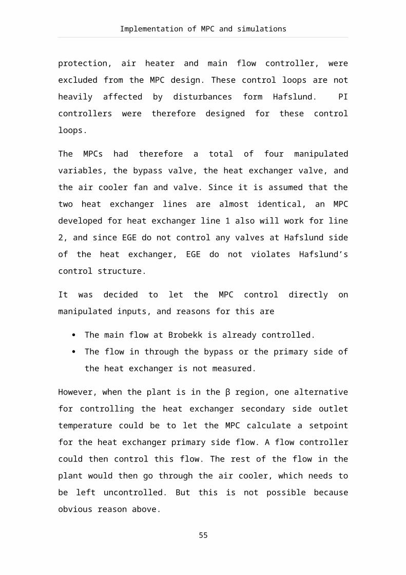
Implementation of MPC and simulations
opens slowly and the bypass valve is used to control the furnace inlet temperature.
Figure 6.29 shows the heat demand form Hafslund, the air cooler primary side outlet
temperature, and the MPC used. When the heat demand from Hafslund drops below 32
MW, the plant enters sub region 1, and thus the MPC developed for this region is used.
When the air cooler primary side outlet temperature goes above the furnace inlet
temperature, the control system enters sub region 2 and switches to the MPC developed
for this region. The switching between the different regions are marked with arrows.
1.4 1.5 1.6 1.7 1.8 1.9 2
x 104
122
124
126
128
130Furnace inlet temperature
Time [s]
[o C]
0 0.2 0.4 0.6 0.8 1 1.2 1.4 1.6 1.8 2
x 104
105
110
115
120
125Outlet temperature - Heat exchanger secondary side
Time [s]
[o C]
Outlet temperatureSetpoint from Hafslund
(a) 1.4 1.5 1.6 1.7 1.8 1.9 2
x 104
122
124
126
128
130Furnace inlet temperature
Time [s]
[o C]
1.4 1.5 1.6 1.7 1.8 1.9 2
x 104
106
108
110
112Outlet temperature - Heat exchanger secondary side
Time [s]
[o C]
Outlet temperatureSetpoint from Hafslund
(b)
Figure 6.27: Figure (a) shows furnace inlet temperature and figure (b) shows the heat exchanger secondary side outlet temperature. Switching from α to β.
57

Implementation of MPC and simulations
1.4 1.5 1.6 1.7 1.8 1.9 2
x 104
0.7
0.8
0.9
1
1.1Heat exchanger valve
Time [s]
Val
ve o
peni
ng [0
-1]
1.4 1.5 1.6 1.7 1.8 1.9 2
x 104
0
0.5
1Bypass valve valve
Time [s]
Val
ve o
peni
ng [0
-1]
1.4 1.5 1.6 1.7 1.8 1.9 2
x 104
0
5000
10000Air cooler fan
Time [s]
[W]
1.4 1.5 1.6 1.7 1.8 1.9 2
x 104
0
0.5
1Air cooler valve
Time [s]
Val
ve o
peni
ng [0
-1]
Figure 6.28: Manipulated variables. Switching from α to β.
58

Implementation of MPC and simulations
1.4 1.5 1.6 1.7 1.8 1.9 2
x 104
28
30
32
34
36Heat demand from Hafslund
Time [s]
[MW
]
1.4 1.5 1.6 1.7 1.8 1.9 2
x 104
0
50
100
150
200Outlet temperature - Air cooler primary side
Time [s]
[o C]
1.4 1.5 1.6 1.7 1.8 1.9 2
x 104
0
1
2
3
4MPC used
Figure 6.29: Heat demand from Hafslund, Temperature in the Air cooler and MPC used. Switching from α to β.
6.4.4 TRANSITION FROM BETA TO ALPHA REGION
When the plant enters the α region, the only control objective is to control the furnace
inlet temperature. EGE should close the air cooler fan and valve, and open the bypass
valve. The plant enters the α region when the heat demand from Hafslund goes above
32 MW, and this can be seen in Figure 6.32. Figure 6.30 shows that transition from the
β region to the α region worked well, the furnace inlet temperature varies some, but the
maximum deviation is about 1°C. Figure 6.31 shows that the air cooler valve and fan
closes while the bypass valve opens, the bypass valve opens exactly when Brobekk
enters the α region.
59

Implementation of MPC and simulations
0 500 1000 1500 2000 2500 3000 3500 4000124.5
125
125.5
126
126.5Furnace inlet temperature
Time [s]
[o C]
0 500 1000 1500 2000 2500 3000 3500 4000107
108
109
110
111Outlet temperature - Heat exchanger secondary side
Time [s]
[o C]
(a) 0 500 1000 1500 2000 2500 3000 3500 4000124.5
125
125.5
126
126.5Furnace inlet temperature
Time [s]
[o C]
0 500 1000 1500 2000 2500 3000 3500 4000107
108
109
110
111Outlet temperature - Heat exchanger secondary side
Time [s]
[o C]
(b)
Figure 6.30: Figure (a) shows furnace inlet temperature and figure (b) shows the heat exchanger secondary side outlet temperature. Switching from β to α.
60
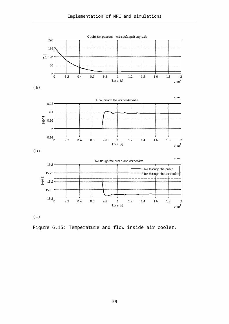
Implementation of MPC and simulations
0 500 1000 1500 2000 2500 3000 3500 40000.98
0.99
1
1.01Heat exchanger valve
Time [s]
Val
ve o
peni
ng [0
-1]
0 500 1000 1500 2000 2500 3000 3500 40000
0.5
1Bypass valve valve
Time [s]
Val
ve o
peni
ng [0
-1]
0 500 1000 1500 2000 2500 3000 3500 40000
5000
10000Air cooler fan
Time [s]
[W]
0 500 1000 1500 2000 2500 3000 3500 40000
0.2
0.4Air cooler valve
Time [s]
Val
ve o
peni
ng [0
-1]
Figure 6.31: Manipulated variables. Switching from β to α.
61

Implementation of MPC and simulations
0 500 1000 1500 2000 2500 3000 3500 400028
30
32
34
36Heat demand from Hafslund
Time [s]
[MW
]
0 500 1000 1500 2000 2500 3000 3500 40000
1
2
3
4MPC used
Figure 6.32: Heat demand from Hafslund and MPC used. Switching from β to α.
62

Implementation of MPC and simulations
63

Conclusion
7 CONCLUSION
The main focus if this work has been to implement a Model Predictive Control at
Brobekk waste incineration plant, in addition the model of the plant had to be modified,
due to physical modification at Brobekk. Based on the operational aspects at Brobekk,
the control region was divided into two distinct regions, named α and β, where the β
region could be divided into four different sub regions. Four different MPCs were
developed, one for the α region, one for each sub region, except sub region 4.
Unfortunately, no simulations were done for the sub region 3, due to the difficulties
with forcing the model to enter this region.
Considerations of the different MPCs developed in this thesis; it seems that all of them
give promising control over the furnace inlet temperature and the heat exchanger
secondary side outlet temperature. In alternative 1 for the β region, the control structure
developed here seems to promise good control of both the furnace inlet temperature and
the temperature towards Oslo, satisfying both EGE’s and Hafslund’s demands. In
alternative 2 for the β region, it was found that the bypass valve at Hafslund’s side
interferers with the temperatures within Brobekk, causing more variations in the furnace
inlet temperature. But the temperature towards Oslo follows its setpoint excellently.
Since we assume that it is more important to have a constant furnace inlet temperature
then it is to follow the setpoint to Hafslund, we suggest using alternative 1.
An alternative is to still use alternative 2, and then let the Hafslund bypass valve be
“slowly” tuned. This might decrease the variations in the furnace inlet temperature and
heat exchanger secondary side outlet temperature. But it is unknown how “slow” the
bypass valve should be tuned, and probably the performance will not be better than in
alternative 1.
Overall, it is concluded that the proposed control structure controls the plant very well,
when EGE only controlling valves at Brobekk side of the heat exchanger.
Based on this work, the following topics can be investigated in further work.
64
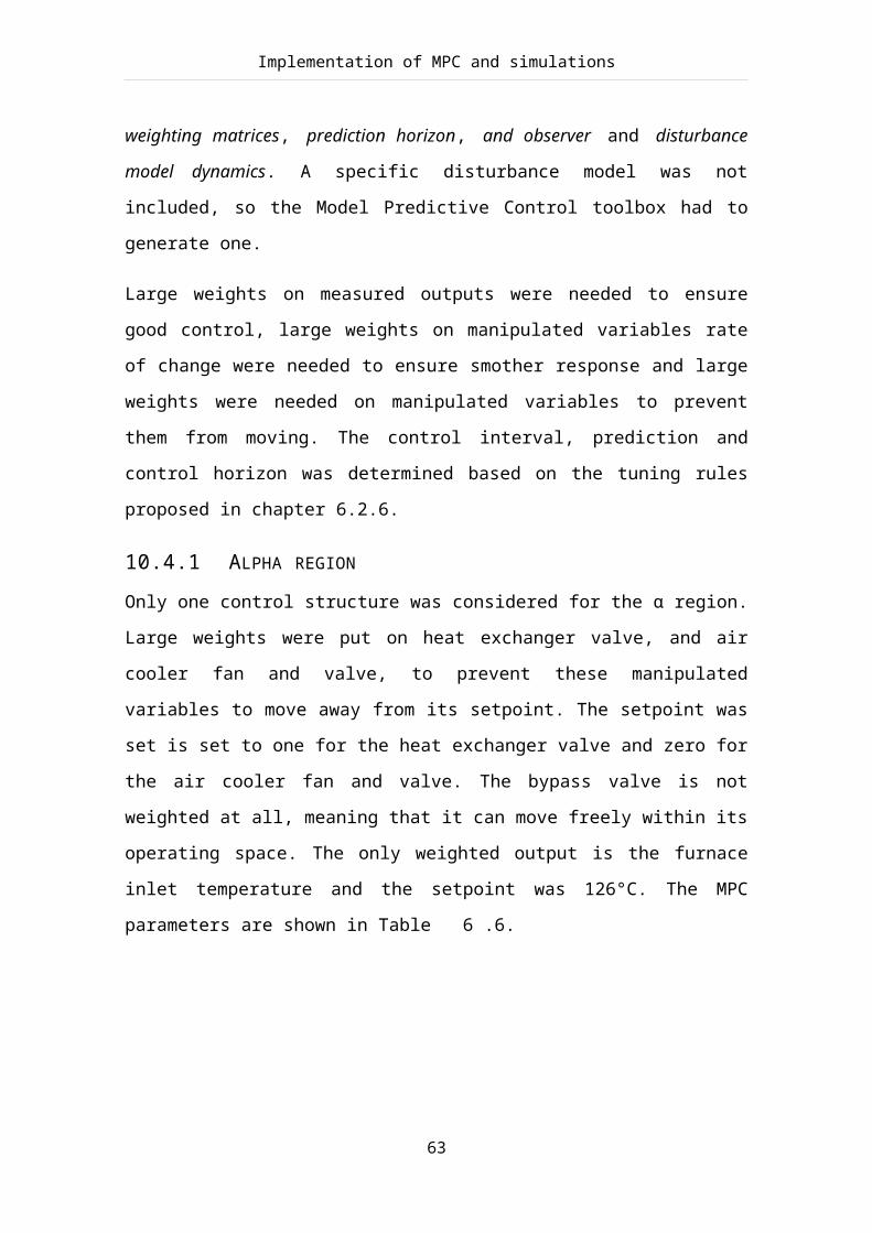
Conclusion
Investigate how additional tuning for the observer and disturbance model can
improve the control even more.
Investigate how the transition between the two regions can be improved. Maybe
if the temperature and flow from the air cooler are measured as a disturbance can
improve the control.
65

Bibliography
8 BIBLIOGRAPHY
Froisy, J. B. (1994). Model predictive control: Past, present and future. ISA
Transactions, 33, 235–243.
Hertzberg, T. (2008). Lecture notes.
Hovd, Morten. (2009). Model-based predictive control. Lecture notes from the course
Advanced Control of Industrial Processes, Department of Engineering Cybernetics,
NTNU.
Imsland, Lars. (2007). Introduction to Model Predictive Control. Lecture notes from the
course Optimization and Control, Department of Engineering Cybernetics, NTNU.
Kern, D.Q. (1950). Process Heat Transfer. McGraw-Hill, int. Ed.
Maciejowski, J. M. (2002). Predictive Control with Constraints. Prentice Hall.
Markus, L. & Lee, E. (1967). Foundations of optimal control theory. J. Wiley, New
York.
Mathisen, K.W. (1994), Integrated design and Control of Heat exchanger Networks.
PhD thesis, NTH, Department of Chemical Engeineering..
Mordt, H. (2010), Private correspondence.
Qin, S. J. & Badgwell, T. A. (2003). A survey of industrial model predictive control
technology. 03, 733–765.
Rosenbrock, H.H. (1970). Process Control System, 2nd edition. McGraw-Hill, USA,
227-230.
Shinskey, F.G. (1979). Process Control System 2nd edition. McGraw-Hill, USA, 227-
230.
Skogestad, S. (2003). Simple analytic rules for model reduction and PID controller
tuning. Journal of Process Control 13 (2003) 291-309.
66
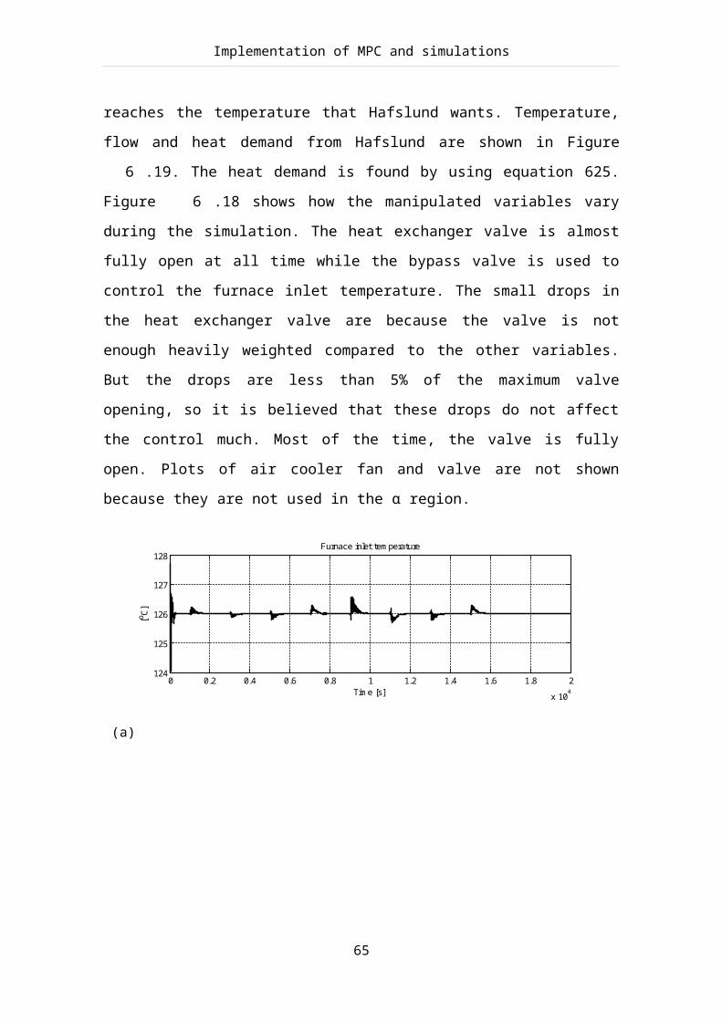
Bibliography
Skogestad, S. (2004). Control structure design for complete chemical plant. Computers
and Chemical Engineering 28 (2004) 219-234.
Skogestad, S. & Postlethwaite, I. (2005). Multivariable Feedback Control. John Wiley
& Sons, Ltd, 2nd edition. 2007.
Smedsrud, H. (2007). Dynamic Model and Control of heat exchanger networks. 5 th year
project work at the Department of Chemical Engineering. NTNU
Smedsrud, H. (2008). Dynamic Modeling and Control of Brobekk Incineration Plant.
Master thesis at the Department of Chemical Engineering. NTNU
The MathWorks, Inc. (2004). Model Predictive Control Toolbox, user guide, v2, 2004
http://www.chbe.gatech.edu/lee/chbe6400_2006/files/mpc_toolbox.pdf
Ziegler, J.G. & Nichold, N.B. (1943). Process Lags in Automatic-Control Circuits.
Trans. ASME, 65, 433-44
67

Appendix
APPENDIX A - LIST OF SYMBOLS
Latin symbolsSymbol Description UnitA Area m2
cp Specific heat capacity J kg-1 K-1
d Disturbance ...h Heat transfer coefficient W m-2 K-1
N Number of cells -P Power Wp Pressure Paq Conducted heat WQ Volumetric flow rate m3 h-1
T Temperature °Ct Time Secondu Manipulated variable ...V Volume m3
w Mass flow rate kg s-1
y Measured variable ...
Greek symbolsSymbol Descriptio
nUnit
η efficiency ...ρ Density kg m-3
Superscript symbolsSymbol
Description
p Primary sides Secondary sidew Wall side
Subscript symbolsSymbol Descriptionin Inlet
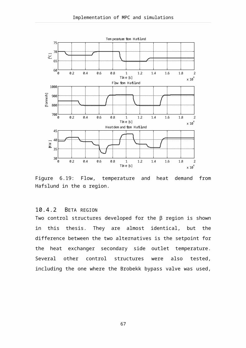
Appendix
out Outlet

Appendix
APPENDIX B - MODEL PARAMETERS
The tables below contain the parameters that were used in the simulations.
General parameters. Heat exchangers parameters.Symbol Value Unit Symbo
lValue Unit
912.892 kg m-3 A 74.6 m2
859.049 kg m-3 Vp 0.2667 m3
80300 kg m-3 Vs 0.3492 m3
0.9285 kg m-3 Vw 0.3730 m3
1.161 kg m-3 N 10 -
1000 kg m-3 hp 9796.09 W m-2 K-1
4321.84 J kg-1 K-1 hs 9796.09 W m-2 K-1
4213.84 J kg-1 K-1
5030 J kg-1 K-1
1018.5 J kg-1 K-1
Air cooler parameters. Air heater parameters.Symbol Value Unit Symbol Value UnitA 74.6 m2 A 30.71 m2
Vp 0.2667 m3 Vp 0.12656 m3
Vs 0.3492 m3 Vs 0.12656 m3
Vw 0.3730 m3 Vw 0.3730 m3
N 10 - N 3 -hp 9796.09 W m-2 K-1 hp 25 W m-2 K-1
hs 9796.09 W m-2 K-1 hs 51 W m-2 K-1
Tair3 0 °C wair4 6 kg s-1
Tair1 0 °C
3 Secondary side inlet temperature to the air cooler and air heater.4 Secondary side flow through the air heater. This was set to be a fixed value.

Appendix
Furnace parameters. Flow factors.Symbol Value Unit Symbol Value UnitUA 52250.6 W K-1 Kv,u5 92.528 m3 h-1 bar-1
Tair 1 1000 °C Kv,u6 83.303 m3 h-1 bar-1
wair 19.86 kg s-1 Kv,u7 260.321 m3 h-1 bar-1
Kv,u8 260.321 m3 h-1 bar-1
Fan parameters. Pump parameters.Symbol Value Unit Symbol Value Unit∆p 1000 Pa p0 15 barTair 0 °C η 0.9 -A 3.14 m1
z 0.6 -η 0.9 -
DisturbancesSymbol Value Unitd1 65-90 °Cd2 500-900 tonne/h

Appendix
APPENDIX C - OPEN LOOP STEP RESPONSES
Open loop responses used to find tuning parameters for PI controllers0 2000 4000 6000 8000 10000 12000 140000
1000
2000
3000
4000
5000From: u7 To: y6Step Response
Time (sec)
Ampl
itude
0 50 100 150 200 250 300 350 400 450 5000
20
40
60
80
100From: u5 To: y3Step Response
Time (sec)
Ampl
itude
0 20 40 60 80 100 120 140 160 180 2004
4.5
5
5.5x 10
-3 From: u1 To: y2Step Response
Time (sec)
Ampl
itude
Figure C.1: Open loop step response for air heater.
0 2000 4000 6000 8000 10000 12000 140000
1000
2000
3000
4000
5000From: u7 To: y6Step Response
Time (sec)
Ampl
itude
0 50 100 150 200 250 300 350 400 450 5000
20
40
60
80
100From: u5 To: y3Step Response
Time (sec)
Ampl
itude
0 20 40 60 80 100 120 140 160 180 2004
4.5
5
5.5x 10
-3 From: u1 To: y2Step Response
Time (sec)
Ampl
itude
Figure C.2: Open loop step response for Air cooler – frost protection.
0 2000 4000 6000 8000 10000 12000 140000
1000
2000
3000
4000
5000From: u7 To: y6Step Response
Time (sec)
Ampl
itude
0 50 100 150 200 250 300 350 400 450 5000
20
40
60
80
100From: u5 To: y3Step Response
Time (sec)
Ampl
itude
0 20 40 60 80 100 120 140 160 180 2004
4.5
5
5.5x 10
-3 From: u1 To: y2Step Response
Time (sec)
Ampl
itude
Figure C.3: Open loop step response for main flow controller.