128 TRANSPORTATION RESEARCH RECORD 1320

Flow and Capacity Characteristics on Two-Lane Rural Highways

ABISHAI PoLus, JosEPH CRAus, AND MosHE LrvNEH

Traffic operation on two-lane rural highways is unique; no lane change is permitted, and overtaking and passing are possible only in the opposing lane of the oncoming traffic. Traffic flow and capacity characteristics on two-Jane highways were investigated. Several models were developed for the relationships between flow parameters. The relationships varied from one road to another and were dependent on the characteristics of each site. Thus, the hourly capacity volume is not a clear, single value. It primarily depends on the geometric and traffic characteristics of the high­way section and on the time interval for which the flow data are collected. The two-way hourly capacity value was found to be about 2,650 passenger cars per hour in both directions . This value was close to the general (extended section) capacity given in the Highway Capacity Manual (HCM) for conditions similar to those in this study. The speeds at which capacity occurs, on the other hand, were lower than the HCM values: about 40 km/hr versus about 70 km/hr. Further research on the proper time interval for an analysis of highway capacity and on flow regimes and capacity values for various geometric, terrain, and traffic characteristics is suggested.

Traffic operation on two-lane rural highways is unique: no lane change is permitted, and overtaking and passing are pos­sible only in the opposing lane of oncoming traffic. This sit­uation results in interaction and influence between the two traffic directions. For example, as the ability to pass declines, drivers are forced to adjust their individual speeds.

The quality of service on two-lane highways is measured by three main traffic characteristics: average travel speed, percentage time delay, and capacity utilization. The average travel speed reflects the mobility function of the road; speeds over 90 km/hr are often observed on major highways. The percentage time delay reflects both the mobility and the access function. The 1985 Highway Capacity Manual (HCM) (1) defines this delay as the average percentage of time that all vehicles are delayed while traveling in platoons because of the inability to pass. Because it is difficult to measure this delay in the field, an evaluation should be made of the per­centage of vehicles that travel in headways of less than 5 sec and this figure should be used as a surrogate variable. The third level-of-service (LOS) measure is a ratio of the demand flow rate to the capacity of the facility. This measure reflects the ability of drivers to drive in comfort without excess in­teraction with other vehicles .

Traffic flow and capacity characteristics on two-lane high­ways were investigated. To that end , several models that de­velop relationships between flow parameters, such as volume

A. Polus, K&D Facilities Resource Corp., 1021 West Adams, Chicago, Ill. 60607. J. Craus and M. Livneh, Department of Civil Engineering, Israel Institute of Technology, Technion City, Haifa , Israel.

and density, were constructed. The basis for this work was a recent study sponsored by the Israel Public Works Depart­ment (2).

BACKGROUND

Speed-flow and delay-flow relationships for two-lane rural highways, under ideal conditions , have been presented by the HCM (1) and are shown in Figure 1. Ideal conditions on two­lane highways almost never exist, mainly because of the pres­ence of trucks and buses and often because of the restriction imposed by the passing-sight distance. Naturally, both of these parameters have a direct and significant effect on the capacity of two-lane highways.

The methodology to determine capacity on two-lane high­ways is quite different for general terrain segments and for specific sections. Designers are often interested in the capacity of a specific section because it may constitute the critical one, such as the bottleneck of a long stretch of highway. The method for determining the capacity of a specific section is more com­plex than that for a long section because the speed at which capacity is reached is difficult to determine. The HCM (J) provides a model relating the flow rate and speeds at various levels of service. The HCM also gives a model that relates flow rate and speeds, at capacity, as follows:

Sc = 25 + 3.75(VJ1,000)2

where

Sc = speed at which capacity occurs (mph), and Ve = flow rate at capacity (veh/hr).

(1)

The plots of the two models yield two curves that intersect . This intersection defines the flow rate at capacity and the speed at capacity for a specific two-lane rural section. An example is shown in Figure 2.

The capacity suggested by the new HCM (1) for two-lane rural highways is 2 ,800 passenger vehicles per hour, both directions, under ideal conditions. The old HCM (3) gave an ideal value of 2,000 passenger vehicles per hour. Most other studies in recent years have reported flows of more than 2,000 veh/hr. Yager's ( 4) survey of various studies showed values for two-directional flows ranging between 3,550 and 2,070 veh/hr.

The measurement of capacity is affected by traffic com­position, particularly the presence of large trucks in the traffic stream. Capacity estimates are also sensitive to the assumed general form of the data and to inherent problems in the curve

Po/us et al.

iOO

90

>< 80

:i ~70

~ 60

~ 50

~ e:J 40 ~

~ 30

20

10

,-' ,/

,/'/

,-'

,/

,' ,'

I , . . I

' ,'

___ ,., ... ----~--~--~~--'--------~ o 0 600 1200 l800 2400 3000

TWO-WAY VOLUME, PCPH

-------- - - - - -------~--~ --

DELAY

0 600 1200 1800 2400 3000

129

fitting of speed-volume data. Duncan (5) discusses the dangers of converting speed-concentration (density) data to speed­flow data. The danger exists particularly if the original data are composed of two different groups: one of free-flowing vehicles and the other of queued vehicles, the behavior of which is not relevant to capacity.

The measurement of capacity is also dependent on the time interval for which data are collected. The intervals should not be too short (e.g., 1 min) because capacity may be overes­timated. If the interval is too long (e.g., 1 hr), capacity will probably be underestimated because the demand may not be sufficient to provide saturation flows for the entire hour. This problem has been addressed by an Organization for Economic Cooperation and Development (OECD) Scientific Expert Group (6), which suggests that the time interval should be the longest possible period consistent with upstream demand.

It is clear, then, that the exact value of capacity is not easily determined. In fact, this measurement is so sensitive that it may vary on the basis of traffic demand fluctuations, short variations in speeds and traffic compositions, and other ran­dom phenomena (such as weather). In light of this variability, it can be argued that the exact value of capacity is of lesser importance in the design process of two-lane roads. Rather, it is of interest in determining the flow rates for the different levels of service, particularly LOS C and D, which often serve as design levels of service.

DATA COLLECTION AND PRELIMINARY OBSERVATIONS

TWO-WAY VOLUME, PCPH

FIGURE 1 Speed-flow and delay-flow relationships at ideal conditions on two-lane rural highways (1).

Data for this study came from two busy two-lane highways in Israel. The two sites were initially selected because the average daily traffic (ADT) was in excess of 10,000 veh/day and, hence, the probability of obtaining dense flow conditions was high. Data were collected only during the midweek peak periods of each section. A video camera positioned at a high point at each site enabled the taping of a continuous section of about V2 km in length. The camera was equipped with a digital clock having an accuracy of 1/100 sec.

559---'T""""-r----- r-------.-----

~ 50 ----t----t-----------------a. Upgrnde speed vs. flow g 45t----"~t----:jt"----"'---...,-----t----~

~ 40 t---+--311i:t-----+-----t----~

"' 35

~ ~

0 300 500 1000 1500 2000 SERVICE FLOW RATE (vph)

lnlersection of Capacily speed vs. flow curve wilh Service Flow Rale

vs. Speed curve defines Cnpncily, SFE' and Speed al Capncily, Sc

2500 2800

FIGURE 2 Use of HCM method to determine capacity of a specific grade.

130

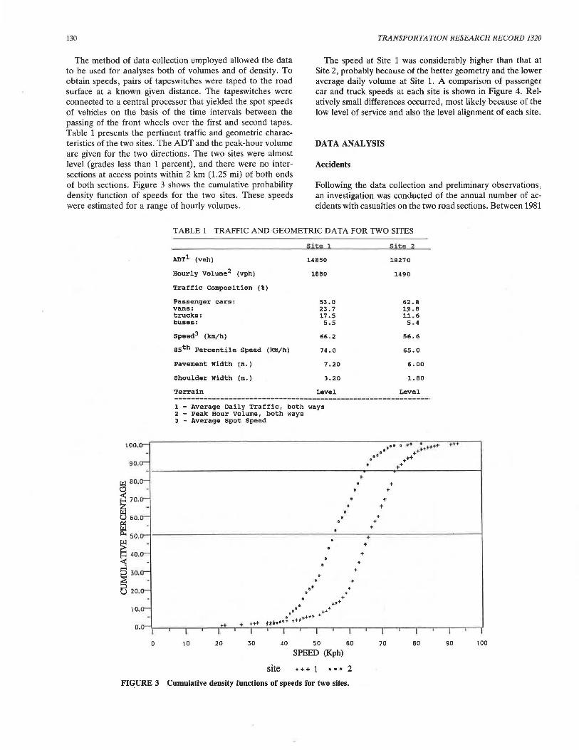
The method of data collection employed allowed the data to be used for analyses both of volumes and of density. To obtain speeds, pairs of tapeswitches were taped to the road surface at a known given distance. The tapeswitches were connected to a central processor that yielded the spot speeds of vehicles on the basis of the time intervals between the passing of the front wheels over the first and second tapes. Table 1 presents the pertinent traffic and geometric charac­teristics of the two sites. The ADT and the peak-hour volume are given for the two directions. The two sites were almost level (grades less than 1 percent), and there were no inter­sections at access points within 2 km (1.25 mi) of both ends of both sections. Figure 3 shows the cumulative probability density function of speeds for the two sites. These speeds were estimated for a range of hourly volumes.

TRANSPORTATION RESEARCH RECORD 1320

The speed at Site 1 was considerably higher than that at Site 2, probably because of the better geometry and the lower average daily volume at Site 1. A comparison of passenger car and truck speeds at each site is shown in Figure 4. Rel­atively small differences occurred, most likely because of the low level of service and also the level alignment of each site.

DATA ANALYSIS

Accidents

Following the data collection and preliminary observations, an investigation was conducted of the annual number of ac­cidents with casualties on the two road sections. Between 1981

TABLE 1 TRAFFIC AND GEOMETRIC DATA FOR TWO SITES

100.

9 0.

~BO.

~ 70

~ 60. (.1.l i:i.. 50.

~ ~ o. < ~ 30;

-

a 20.

10.

o.

0

:Ut!i! l

ADT1 (veh) 14850

Hourly Volume2 (vph) 1880

Traffic Composition (%)

Passenger cars: 53.0 vans: 23.7 trucks: 17.5 buses: 5.5

Speed3 (km/h) 66.2

95th Percentile Speed (km/h) 74.0

Pavement Width (m. l 7.20

Shoulder Width (m.) 3.20

Terrain Level

1 - Average Daily Traffic, both ways 2 - Peak Hour Volume, both ways 3 - Average Spot Speed

~it!il Oil

18270

1490

62 . 8 19.8 11. 6

5 . 4

56.6

65.0

6.00

1.80

Level

• +

10 20 30

• +

+ +

• + • +

. . ...

40 50 60

SPEED (Kph)

site + ... + 1 • e • 2

+

... +

+ +

+

70 80

FIGURE 3 Cumulative density functions of speeds for two sites.

...

90 100

Po/us et al.

~

~ 5 c:: IE

~

100.0-

•O.

10.

10.

60.

so.

•o. lO,

10.

ID,

e+ e+ +

+ i

131

i 0,

Cl> .+*-1#-++~

.,11c1 1111>1+

10 20 lO '° so 10 10 80 100

SPEED (Kph)

type of vehicle : +++ passenger car 0 0 0 tnx:k

100.

~ 90.

~ 10.

lo.

c:: so.

IE , .. .,...

I •0.

N.

20,

a 10.

o.o

10 20 lO

e e +If e +-+'

e / e +

+ e /

++ e

10

SPEED (Kph) 70 10 ID 100

type of vehicle : +++ passenger car 0 0 0 tnx:k

FIGURE 4 Cumulative density functions of speeds of cars and trucks for sites 1 and 2.

and 1985, the average number of accidents was 2.6 at Site 1 and 8.0 at Site 2. This difference was attributed to the im­proved geometry of Site 1, which included full, 7.20-m pave­ment with 3.0-m clear shoulders on each side.

Speed-Volume Relationship

The speed-volume relationship is often shown as a parabolic curve. The results obtained for this study are shown in Figure 5. The data at Site 2 result in a clear parabolic shape with a distinct peak, which indicates capacity. At Site 1, no peak was observed, and data were obtained only on the upper part of the curve.

These observations show two important findings. First, the flow regime at Site 2 is in the vicinity of capacity, above and below the maximum volume of about 420 vehicles per 15 min (both ways). At Site 1, the flow is below capacity, although some high volumes are obtained (more than 600 vehicles in

15 min). Second, the capacity zone at Site 2 occurs at a wide range of speeds, about 25 to 45 km/hr. This finding demon­strates that capacity on two-lane roads is a value that is not obtained at only one point on the speed-volume curve. It further shows that the flow data do not always behave ac­cording to the theoretical parabolic model. The relationship varies from one road to another and is dependent on the characteristics of each site.

Therefore, the hourly capacity volume is not a clear, single value. Furthermore, it is dependent on the time interval for which the data are collected . Naturally, a capacity based on 1-min observations will be higher than one based on 10- or 15-min time intervals. High capacity values may be obtained for short periods of time (i.e., short time intervals) because of flow characteristics: traffic on two-lane rural roads may flow with short headways (and therefore high volumes) only for short periods. As the time interval of the observation increases, the flow becomes inconsistent because average headways grow, as does the variation between headways. The

132

BO

I I I I I I I I I 1

50 lDD 150 2DD 250 30D 350 4DO 45D 5DD 55D 6DO

VOLUME (vp 15 min)

site= 1

BO

7D

~:g: ~o

-i:r.fll'"1Jt1:i.i ei~ 50 ' ft llleJ 40 '~t o< ~i:i.. 30

*Ill' ~Cl)

20 <~

10

SD 1 DO 1 SD 2DD 250 300 350 400

VOLUME (vp 15 min)

site= 2

FIGURE 5 Speed-volume relationships for sites 1 and 2.

hourly volume, which is calculated from a longer time interval, therefore decreases .

Hourly capacity volumes are presented in Tables 2 and 3. The maximum one-way hourly volume shown in Table 2 for Site 1 is 1,980 veh/hr calculated from 1-min lime intervals and 1,448 veh/hr calculated from 15-min intervals, or about a 37 percent difference. Table 3 presents the two-way maximum hourly volumes for the two directions together; the observed speeds obtained at capacity vary only slightly.

It is interesting to compare the observed capacity values with the HCM (1) values. To do so, the 15-min time intervals were used because the HCM analysis is based on observations at these intervals. The traffic directional split in this study was 60-40, and the percentage of trucks during the observa-

TRANSPORTATION RESEARCH RECORD 1320

TABLE 3 MAXIMUM FLOW VALUES FOR BOTH DIRECTIONS AND VARIOUS TIME INTERVALS

Time Interval (min.)

1

5

10

15

v max

48

212

392

580

VPH

2880

2544

2352

2320

s (km/h)

55

55

57

58

- Max. measured volume for the specified time interval

VPH - Calculated hourly volume, both directions

B - Obacrvcd apace mean apccd at capacity

tions was approximately 14 percent. To convert the calcu­lated, mixed two-way maximum hourly volume (2,320 veh/ hr) to an equivalent hourly passenger car volume , a passenger car equivalent of 2 was used (level terrain) . This calculation gave a maximum hourly volume of 2,645 veh/hr. The HCM value (directional split of 60-40, as shown on HCM page 8-6) is 2,650 passenger cars per hour, in both directions . The proximity of the two-way capacity values from this study and the HCM is evident .

The speeds, on the other hand, are not similar. The HCM gives a speed of about 72 km/hr (45 mph) as the speed at capacity (see HCM Figure 8-1). The average speed in this study was about 58 km/hr, and the speed at capacity was even lower (about 40 km/hr) . It is concluded that , although the capacity values obtained by the HCM seem adequate, the speeds at which they occur are more sensitive to the geometric conditions of lht: roadway and may be lower than HCM­suggested values.

Speed-Density Relationship

Further analysis was conducted of the density data collected at Site 1. The speed-density curve shown in Figure 6 was based on average 15-min densities for a 1-km (0.62-mi) section. The densities varied widely between 10 vehicles per kilometer

TABLE 2 VOLUMES FOR VARIOUS INTERVALS AND CALCULATED HOURLY VOLUMES

Tim.a SITE 1 SITE 2 Interval 1st Di rect i on 2Dd Direct ion 1st Direction 2nd Direction (min.)

v VPH v VPH v VPH v VPH max max max max -·-------------------------------------------------------------------------

l 30 1800 33 1980 23 1386 19 1140

5 132 1584 103 1236 96 1152 60 720

10 239 1434 195 1170 185 1110 105 630

15 362 1448 276 1104 276 1104 196 584

Vmax - The maximum volume, as measured for a specified time interval

VPH - Calculated hourly volume

Po/us et al.

ao -

~ 70-

~ so-

so -~ 40 -

~ 30 -Cl)

i 20-

10 -

< o-I

0 5

I

10 '

15

I

20

I

25 '

30 35

133

DENSITY (vpkm) 15

FIGURE 6 Speed-density relationship for Site 1.

(vpkm) and about 30 vpkm, which further indicates that traffic flow may be dense at certain times and light at other periods.

Volume-Density Relationship

The volume-density relationship for Site 1 is shown in Figure 7. There is a volume increase with 15-min interval observa­tions as the density increases. The data spread is such that the resultant slope at high densities (about 25 vpkm) is smaller than that at low densities (about 15 vpkm) . This finding in­dicates that a maximum volume was not reached at Site 1, as shown in Figure 5. Although the common volume-density relationship is parabolic, the peak volume could not be de­tected at high densities. The relationship between volume V in veh/hr and density D in vpkm can be expressed as a par­abolic relationship as follows:

V = aD2 + bD + c (2)

in which a, b, and care constants . Calibration of this equation was performed on the volume­

density data for various time intervals , and the results are

600-

sso -500 -

1450-

"" 400 -..... 350 -

~ 500 -

~ 2so ­S 200-

cl 1 so -> 100 -

so -

presented in Table 4. The correlation coefficient increases with the increase in the time interval. This result is probably due to the reduction in variability of the data with the increase of the time period for which the data were collected.

CONCLUSIONS

Several conclusions can be drawn from this study. First, as expected, the capacity value is sensitive to the geometric char-

TABLE 4 CORRELATION COEFFICIENTS AND PARAMETERS OF VOLUME-DENSITY RELATIONSHIP

Time Interval (min.)

a b c __________________________ , ___________________ ______

l o.oo 0.11 21.20 0.22

5 -0.06 7.16 24.04 0.62

10 -0.26 20.90 -27.16 0.76

15 -0.47 35.46 -87.86 0.83

o-~, ~-,...~-,.------.~--.,~---.-~-.-~--.-~~,,...----.~-...-, ~r-~,.------.~_.,.

o s 1 o 1 s 20 25 30 35

DENSITY (vpkm)

FIGURE 7 Volume-density relationship for Site 1.

134

acteristics of each site. Second, continuously changing traffic characteristics, such as the percentage of trucks, the direc­tional split, the presence of a vehicle on the shoulder, or even the occurrence of a potential incident during dense flow con­ditions, have a great impact on road capacity. The flow re­gime, whether below or above HCM capacity, is very sensitive to the specific traffic conditions at any given time interval. Third, the value of capacity is highly dependent on the time interval for which data are collected and from which the ca­pacity is calculated. A practical finding was that the capacity value, as calculated for 15-min time intervals, was similar to the HCM value. The speed at which this capacity occurs, however, was lower than the general speed recommended by the HCM.

Further research is suggested on two subjects. At the the­oretical level, a calculation should be made of the proper time interval for an analysis of capacity. At the empirical level, investigation should be made of flow regimes and capacity values for various geometric conditions, terrains, and traffic characteristics.

TRANSPORTATION RESEARCH RECORD 1320

REFERENCES

1. Special Report 209: Highway Capacity Manual. TRB, National Research Council, Washington, D.C., 1985.

2. A. Polus, J. Craus, M. Livneh, and M. Gross. Analysis of Capacity and Dense Flow Characteristics on Two-Lane Highways. Research Report 88-125. Transportation Research Institute, Technion­Israel Institute of Technology, Haifa, July 1988.

3. Special Report 87: Highway Capacity Manual. HRB, National Research Council, Washington, D.C., 1965.

4. S. Yager. Capacities for Two-Lane Highways. Austrnlian Road Research Board, Vermont South, Victoria, March 1983.

5. N. C. Duncan. A Further Look at Speed/Flow/Concentration Traffic Engineering and Control. Traffic Engineering and Control, Vol. 20, No. 10, Oct. 1979, pp. 482-483.

6. OECD Scientific Expert Group. Traffic Capacity of Major Routes. Road Transport Research, Organization for Economic Coopera­tion and Development, Paris, July 1983.

Publication of this paper sponsored by Committee on High way Capacity and Quality of Service.