Embed Size (px)
Citation preview
i
This degree project was done in cooperation with Nordicstation
Mentor at Nordicstation: Christian Isaksson
Flexible Data Extraction for Analysis using Multidimensional Databases and OLAP Cubes
Flexibelt extraherande av data för analys med multidimensionella databaser och OLAP-kuber
TOB IAS HULTGREN ROBERT JERNBERG
Degree Project in
Computer Engineering Undergraduate, 15 Credits
Mentor at KTH: Reine Bergström
Examiner: Ibrahim Orhan School of Technology and Health
TRITA-STH 2013:23
Royal Institute of Technology
School of Technology and Health 136 40 Handen, Sweden
http://www.kth.se/sth

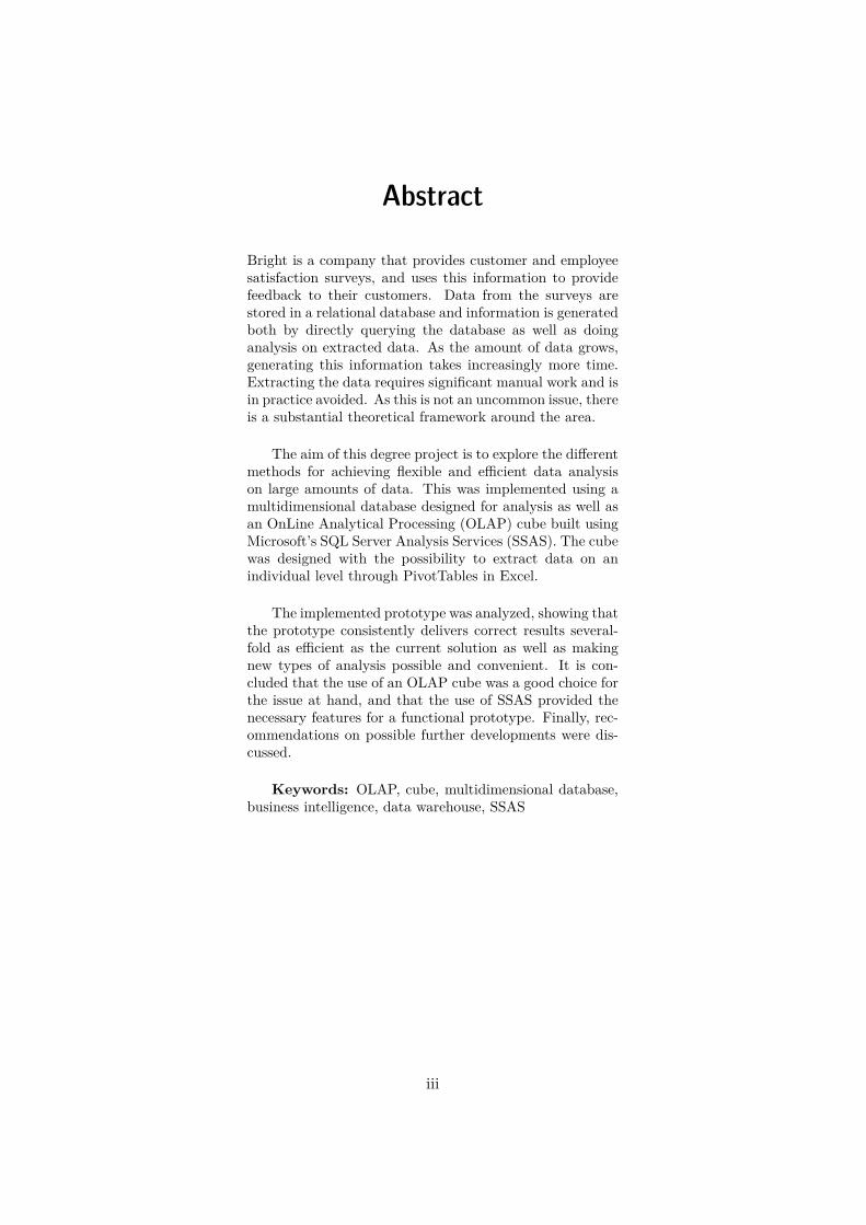
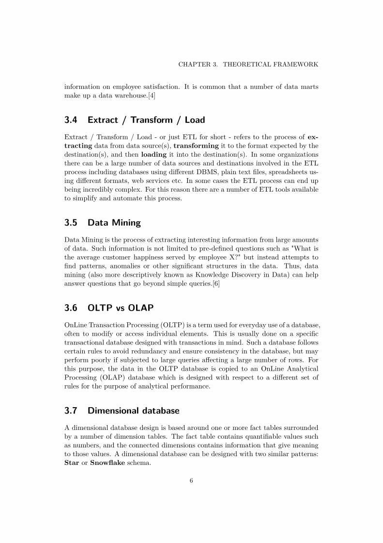
Abstract
Bright is a company that provides customer and employeesatisfaction surveys, and uses this information to providefeedback to their customers. Data from the surveys arestored in a relational database and information is generatedboth by directly querying the database as well as doinganalysis on extracted data. As the amount of data grows,generating this information takes increasingly more time.Extracting the data requires significant manual work and isin practice avoided. As this is not an uncommon issue, thereis a substantial theoretical framework around the area.
The aim of this degree project is to explore the differentmethods for achieving flexible and efficient data analysison large amounts of data. This was implemented using amultidimensional database designed for analysis as well asan OnLine Analytical Processing (OLAP) cube built usingMicrosoft’s SQL Server Analysis Services (SSAS). The cubewas designed with the possibility to extract data on anindividual level through PivotTables in Excel.
The implemented prototype was analyzed, showing thatthe prototype consistently delivers correct results several-fold as efficient as the current solution as well as makingnew types of analysis possible and convenient. It is con-cluded that the use of an OLAP cube was a good choice forthe issue at hand, and that the use of SSAS provided thenecessary features for a functional prototype. Finally, rec-ommendations on possible further developments were dis-cussed.
Keywords: OLAP, cube, multidimensional database,business intelligence, data warehouse, SSAS
iii


Sammanfattning
Bright är ett företag som tillhandahåller undersökningar förkund- och medarbetarnöjdhet, och använder den informa-tionen för att ge återkoppling till sina kunder. Data frånundersökningarna sparas i en relationsdatabas och infor-mation genereras både genom att direkt fråga databasensåväl som att göra manuell analys på extraherad data. Närmängden data ökar så ökar även tiden som krävs för attgenerera informationen. För att extrahera data krävs enbetydande mängd manuellt arbete och i praktiken undviksdet. Då detta inte är ett ovanligt problem finns det ett ge-diget teoretiskt ramverk kring området.
Målet med detta examensarbete är att utforska de oli-ka metoderna för att uppnå flexibel och effektiv dataana-lys på stora mängder data. Det implementerades genom attanvända en multidimensionell databas designad för analyssamt en OnLine Analytical Processing (OLAP)-kub byggdmed Microsoft SQL Server Analysis Services (SSAS). Ku-ben designades med möjligheten att extrahera data på enindividuell nivå med PivotTables i Excel.
Den implementerade prototypen analyserades vilket vi-sade att prototypen konsekvent levererar korrekta resultatflerfaldigt så effektivt som den nuvarande lösningen såvälsom att göra nya typer av analys möjliga och lättanvända.Slutsatsen dras att användandet av en OLAP-kub var ettbra val för det aktuella problemet, samt att valet att an-vända SSAS tillhandahöll de nödvändiga funktionaliteternaför en funktionell prototyp. Slutligen diskuterades rekom-mendationer av möjliga framtida utvecklingar.
v


Acknowledgments
We would like to thank Nordicstation for the opportunity to do our degree projectwith them. Special thanks to Christian Isaksson at Nordicstation for mentoringand technical advice. We would also like to thank Bright for providing the problemthis degree project set out to solve. Special thanks to Kent Norman who was ourcontact at Bright for describing the requirements and giving feedback during thework. Lastly we would like to thank KTH and our lecturers for the education wehave received over these years. Special thanks to Reine Bergström at KTH for hisadvice and mentoring during our degree project.
vii


Abbreviations
BI: Business Intelligence. A set of technologies and methods for extracting rel-evant business intelligence from data sources.
OLAP: On-Line Analytical Processing. A database designed for analytical pur-poses.
OLTP: On-Line Transaction Processing. A database designed for transactionalpurposes.
DBMS: DataBase Management System. A system used to manage a database,such as SQL Server.
ETL: Extract/Transform/Load. A set of actions intended to extract informa-tion from a source, transform it if necessary, and finally load it into a desti-nation.
SQL: Structured Query Language. Language standard for querying databases.This standard is to some degree followed by major DBMS’s.
SSAS: SQL Server Analysis Services. Microsoft’s BI tool for data analysis.
SSIS: SQL Server Integration Services. Microsoft’s BI tool for data migra-tion.
SSRS: SQL Server Reporting Services. Microsoft’s BI tool for producing graph-ical reports.
MDX: MultiDimensional eXpressions. A query language similar to SQL usedto query OLAP databases.
GUI: Graphical User Interface. A graphical user interface used for user inter-action.
API: Application Programming Interface. An interface to application func-tions accessible by other applications.
JDBC: Java DataBase Connectivity. A standard API for SQL database con-nectivity.
ix

XMLA: Extensible Markup Language for Analysis. Industry standard XMLbased language for OLAP.
MOLAP: Multidimensional Online Analytical Processing. Storage modewhere both atomic data and aggregates are stored in the cube.
ROLAP: Relational Online Analytical Processing. Storage mode where bothatomic data and aggregates are stored in the relational database.
x
Contents
1 Introduction 11.1 Background . . . . . . . . . . . . . . . . . . . . . . . . . . . . . . . . 11.2 Goals . . . . . . . . . . . . . . . . . . . . . . . . . . . . . . . . . . . 11.3 Delimitations . . . . . . . . . . . . . . . . . . . . . . . . . . . . . . . 21.4 Solutions . . . . . . . . . . . . . . . . . . . . . . . . . . . . . . . . . 2
2 Current Situation 3
3 Theoretical Framework 53.1 Business Intelligence . . . . . . . . . . . . . . . . . . . . . . . . . . . 53.2 Data Warehouse . . . . . . . . . . . . . . . . . . . . . . . . . . . . . 53.3 Data Mart . . . . . . . . . . . . . . . . . . . . . . . . . . . . . . . . . 53.4 Extract / Transform / Load . . . . . . . . . . . . . . . . . . . . . . . 63.5 Data Mining . . . . . . . . . . . . . . . . . . . . . . . . . . . . . . . 63.6 OLTP vs OLAP . . . . . . . . . . . . . . . . . . . . . . . . . . . . . 63.7 Dimensional database . . . . . . . . . . . . . . . . . . . . . . . . . . 63.8 OLAP Cube . . . . . . . . . . . . . . . . . . . . . . . . . . . . . . . . 7
4 Methods 114.1 Requirements . . . . . . . . . . . . . . . . . . . . . . . . . . . . . . . 114.2 Candidate methods . . . . . . . . . . . . . . . . . . . . . . . . . . . . 12
4.2.1 Modifying the current solution . . . . . . . . . . . . . . . . . 124.2.2 Using an OLAP tool . . . . . . . . . . . . . . . . . . . . . . . 12
4.3 Chosen method . . . . . . . . . . . . . . . . . . . . . . . . . . . . . . 134.4 Tools for the chosen method . . . . . . . . . . . . . . . . . . . . . . . 13
4.4.1 Technical requirements . . . . . . . . . . . . . . . . . . . . . . 134.4.2 Examined tools . . . . . . . . . . . . . . . . . . . . . . . . . . 14
4.4.2.1 Oracle Essbase . . . . . . . . . . . . . . . . . . . . . 144.4.2.2 Microsoft SSAS 2008 R2 . . . . . . . . . . . . . . . 144.4.2.3 Palo 3.2 and Jedox 5.0 . . . . . . . . . . . . . . . . 154.4.2.4 PowerPivot . . . . . . . . . . . . . . . . . . . . . . . 15
4.4.3 Choice of tool . . . . . . . . . . . . . . . . . . . . . . . . . . . 16
5 Implementation 17
xi
5.1 Database conversion . . . . . . . . . . . . . . . . . . . . . . . . . . . 175.1.1 Relevant source data . . . . . . . . . . . . . . . . . . . . . . . 175.1.2 Dimensional database design . . . . . . . . . . . . . . . . . . 18
5.1.2.1 Respondent dimension . . . . . . . . . . . . . . . . . 185.1.2.2 Question dimension . . . . . . . . . . . . . . . . . . 185.1.2.3 Time dimension . . . . . . . . . . . . . . . . . . . . 195.1.2.4 Answers fact table . . . . . . . . . . . . . . . . . . . 19
5.1.3 ETL operations . . . . . . . . . . . . . . . . . . . . . . . . . . 195.2 Data cube implementation . . . . . . . . . . . . . . . . . . . . . . . . 21
5.2.1 Defining dimensions . . . . . . . . . . . . . . . . . . . . . . . 215.2.1.1 Respondent dimension . . . . . . . . . . . . . . . . . 225.2.1.2 Question dimension . . . . . . . . . . . . . . . . . . 235.2.1.3 Time dimension . . . . . . . . . . . . . . . . . . . . 23
5.2.2 Creating the cube . . . . . . . . . . . . . . . . . . . . . . . . 235.3 Interface . . . . . . . . . . . . . . . . . . . . . . . . . . . . . . . . . . 25
5.3.1 User Interface . . . . . . . . . . . . . . . . . . . . . . . . . . . 255.3.2 Application Interface . . . . . . . . . . . . . . . . . . . . . . . 26
6 Analysis 296.1 Aggregate analysis . . . . . . . . . . . . . . . . . . . . . . . . . . . . 296.2 Correlational analysis . . . . . . . . . . . . . . . . . . . . . . . . . . 316.3 ETL operations and cube processing . . . . . . . . . . . . . . . . . . 336.4 Storage size . . . . . . . . . . . . . . . . . . . . . . . . . . . . . . . . 33
7 Conclusions 35
8 Recommendations 378.1 Selective ETL . . . . . . . . . . . . . . . . . . . . . . . . . . . . . . . 378.2 Real-time synchronization . . . . . . . . . . . . . . . . . . . . . . . . 378.3 Redundant questions . . . . . . . . . . . . . . . . . . . . . . . . . . . 388.4 Web interface using the cube . . . . . . . . . . . . . . . . . . . . . . 388.5 Move data warehouse to specific database . . . . . . . . . . . . . . . 398.6 Optimize cube pre-calculated aggregates . . . . . . . . . . . . . . . . 398.7 Server side correlational calculations . . . . . . . . . . . . . . . . . . 40
References 41
xii

Chapter 1
Introduction
1.1 Background
Bright is a company that performs customer and employee satisfaction surveys.They collect answers to questions regarding satisfaction from millions of users forcompanies in different industries, and uses this data to provide feedback to therespective companies on what their customers and employees are satisfied with andalso to investigate what can be done to improve relations with them. These surveysare carried out using the web and automated telephone calls.
Because of the large amounts of data in their relational database it has becomea challenge to extract the sought information, and to do this in a fast and flexibleway.
1.2 Goals
The goal of the task is to develop a solution that can extract the sought informationand to do this in an efficient manner without adversely affecting the customers’ use ofthe database. There are two major kinds of information that are sought; aggregatesand correlations.
Aggregates refers to the summarized information of a specific range of datain the database. For example, the total number of surveys for company X in June2012 or the average general customer satisfaction for company Y in 2013.
Correlations in our case refers to correlations between answers given from onecustomer. For example, ”how does the waiting time for customer support affect thecustomer satisfaction?”. Correlations may also be a correlation between differentaggregates, eg. average waiting time compared to average customer satisfaction, butthe further away from individual surveys the analysis takes place, the less valuable
1

CHAPTER 1. INTRODUCTION
it is for Bright’s analysts.
Furthermore, the solution must be compatible with the in-place systems usedby Bright, which are mostly based on the Microsoft platform.
1.3 DelimitationsThe solution was based on the problems as stated above and the system was devel-oped with Bright’s needs in mind. Feature requests that did not serve to further thedepth of this degree project were left to be implemented on a future improvementbasis. The time span for developing a prototype was limited to six weeks and thegoals were limited to this.
The database provided by the company runs the SQL Server 2008 R2 DBMS.This was the database that was to be used without further analysis of which DBMSmight be optimal for the purpose of data analysis.
With consideration to the great amount of tools available for the purpose ofdata analysis, this degree project will not provide an exhaustive list or review ofeach of them. Only a selection of tools will be briefly reviewed for the purpose ofpicking one that provides the necessary functionalities we require.
1.4 SolutionsThe problem was solved by implementing a dimensional database in SQL Serverand a data cube on top of it using Microsoft SQL Server Analysis Services (SSAS).The dimensional database provides an efficient storage format for large queries aswell as being a format easily used in SSAS. The data cube provides an intuitiveand efficient way of browsing the data with the necessary aggregates available.Extract / Transform / Load (ETL) operations can be run routinely to populatethe dimensional database with up-to-date data from the transactional database.The ETL operations can be run nightly to not adversely affect customer use of thedatabase. All analyses is done on the cube and dimensional database ensuring thatthe transactional database is not adversely affected.
2

Chapter 2
Current Situation
Currently, there are two entities which are using information from the database; theweb interface and internal analysis.
The web interface is accessible by all of Bright’s customers and serves topresent different aggregates; eg. the average customer satisfaction for differentsections in the company. The users can browse different company hierarchies andfilter on time ranges. Which data that can be browsed is pre-defined and rarelychanged. As of now this data is derived partly from specially prepared tables in thedatabase and partly from directly querying the transactional data. Even thoughthe prepared tables speed up the queries it can still take several seconds to executethem when aggregating data for a large company or over a large time span.
The internal analysis serves to let Bright’s analysts further analyze the datato find interesting information and be able to give their customers recommendationson how to improve customer and employee satisfaction. It is also used for internalreporting such as billing. To get all the data needed for the internal analyzing ina useful format, some fairly complex queries has to be run against the database.Much of the work is done using Microsoft Access databases and then copying datainto Excel spreadsheets. As this is done manually, it takes a lot of time and hasto be repeated every time new data is needed. It introduces a risk of human erroreach time the data is handled.
3


Chapter 3
Theoretical Framework
In a field as expansive as Business Intelligence[1], there are many relevant conceptsand technologies. These concepts are briefly explained in the following sections.
3.1 Business IntelligenceBusiness Intelligence (BI) is a generic term which refers to a wide array of technolo-gies and methods used to extract relevant business information from different datasources that can be used to help making informed decisions in a business.[2]
3.2 Data WarehouseWhile a transactional database is intended and designed for processing (mostlysmall) transactions, a data warehouse is intended and designed for processing (oftenlarge) queries and data analysis. It is common that a data warehouse containshistorical information as opposed to a transaction database which may only containsthe current situation.[3, 4]
Why use a Data Warehouse? IBM estimates that, as of January 2012, that90% of the world’s data was created in the past two years. This data comes from allkind of source including purchase transactions, social media and climate informationsensors. Clever solutions are necessary to process this data in an efficient manner inorder to extract relevant information and acquire sought knowledge. This is doneusing a data warehouse which stores all historical data and is designed to processit.[5]
3.3 Data MartA Data Mart refers to stored data for a single business process. For example, oneData Mart can keep information about customer satisfaction, and another can keep
5
CHAPTER 3. THEORETICAL FRAMEWORK
information on employee satisfaction. It is common that a number of data martsmake up a data warehouse.[4]
3.4 Extract / Transform / Load
Extract / Transform / Load - or just ETL for short - refers to the process of ex-tracting data from data source(s), transforming it to the format expected by thedestination(s), and then loading it into the destination(s). In some organizationsthere can be a large number of data sources and destinations involved in the ETLprocess including databases using different DBMS, plain text files, spreadsheets us-ing different formats, web services etc. In some cases the ETL process can end upbeing incredibly complex. For this reason there are a number of ETL tools availableto simplify and automate this process.
3.5 Data Mining
Data Mining is the process of extracting interesting information from large amountsof data. Such information is not limited to pre-defined questions such as "What isthe average customer happiness served by employee X?" but instead attempts tofind patterns, anomalies or other significant structures in the data. Thus, datamining (also more descriptively known as Knowledge Discovery in Data) can helpanswer questions that go beyond simple queries.[6]
3.6 OLTP vs OLAP
OnLine Transaction Processing (OLTP) is a term used for everyday use of a database,often to modify or access individual elements. This is usually done on a specifictransactional database designed with transactions in mind. Such a database followscertain rules to avoid redundancy and ensure consistency in the database, but mayperform poorly if subjected to large queries affecting a large number of rows. Forthis purpose, the data in the OLTP database is copied to an OnLine AnalyticalProcessing (OLAP) database which is designed with respect to a different set ofrules for the purpose of analytical performance.
3.7 Dimensional database
A dimensional database design is based around one or more fact tables surroundedby a number of dimension tables. The fact table contains quantifiable values suchas numbers, and the connected dimensions contains information that give meaningto those values. A dimensional database can be designed with two similar patterns:Star or Snowflake schema.
6
3.8. OLAP CUBE
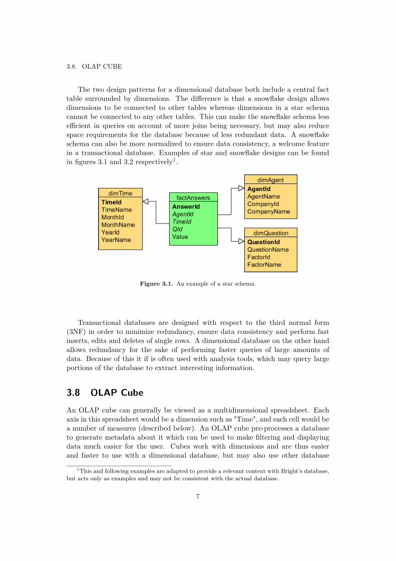
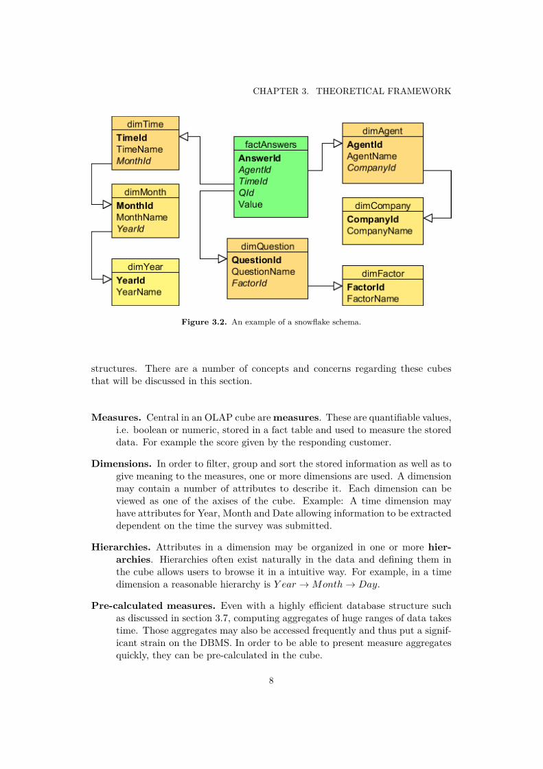
The two design patterns for a dimensional database both include a central facttable surrounded by dimensions. The difference is that a snowflake design allowsdimensions to be connected to other tables whereas dimensions in a star schemacannot be connected to any other tables. This can make the snowflake schema lessefficient in queries on account of more joins being necessary, but may also reducespace requirements for the database because of less redundant data. A snowflakeschema can also be more normalized to ensure data consistency, a welcome featurein a transactional database. Examples of star and snowflake designs can be foundin figures 3.1 and 3.2 respectively1.
Figure 3.1. An example of a star schema.
Transactional databases are designed with respect to the third normal form(3NF) in order to minimize redundancy, ensure data consistency and perform fastinserts, edits and deletes of single rows. A dimensional database on the other handallows redundancy for the sake of performing faster queries of large amounts ofdata. Because of this it if is often used with analysis tools, which may query largeportions of the database to extract interesting information.
3.8 OLAP Cube
An OLAP cube can generally be viewed as a multidimensional spreadsheet. Eachaxis in this spreadsheet would be a dimension such as "Time", and each cell would bea number of measures (described below). An OLAP cube pre-processes a databaseto generate metadata about it which can be used to make filtering and displayingdata much easier for the user. Cubes work with dimensions and are thus easierand faster to use with a dimensional database, but may also use other database
1This and following examples are adapted to provide a relevant context with Bright’s database,but acts only as examples and may not be consistent with the actual database.
7
CHAPTER 3. THEORETICAL FRAMEWORK
Figure 3.2. An example of a snowflake schema.
structures. There are a number of concepts and concerns regarding these cubesthat will be discussed in this section.
Measures. Central in an OLAP cube aremeasures. These are quantifiable values,i.e. boolean or numeric, stored in a fact table and used to measure the storeddata. For example the score given by the responding customer.
Dimensions. In order to filter, group and sort the stored information as well as togive meaning to the measures, one or more dimensions are used. A dimensionmay contain a number of attributes to describe it. Each dimension can beviewed as one of the axises of the cube. Example: A time dimension mayhave attributes for Year, Month and Date allowing information to be extracteddependent on the time the survey was submitted.
Hierarchies. Attributes in a dimension may be organized in one or more hier-archies. Hierarchies often exist naturally in the data and defining them inthe cube allows users to browse it in a intuitive way. For example, in a timedimension a reasonable hierarchy is Y ear →Month→ Day.
Pre-calculated measures. Even with a highly efficient database structure suchas discussed in section 3.7, computing aggregates of huge ranges of data takestime. Those aggregates may also be accessed frequently and thus put a signif-icant strain on the DBMS. In order to be able to present measure aggregatesquickly, they can be pre-calculated in the cube.
8

3.8. OLAP CUBE
Data explosions. In order to pre-calculate all measures, one value for all possibleintersections of the cube dimensions, known as the Cartesian product, wouldhave to be stored. Since this will grow very fast as more dimensions are addedand the number of rows in each dimension increases, the space needed to storeall pre-calculated values can become a problem. This phenomena is know as adata explosion, and OLAP cube tools often have ways to solve this issue.[7]
9

Chapter 4
Methods
As with most problems there are many ways to solve it. Based on the given goalsand circumstances, different methods that could be used were considered. Afterchoosing a method, available tools for the development of a solution were examined.
4.1 Requirements
To be able to meet the given goals of this degree project, the chosen method mustmeet several requirements. These requirements can be divided into three categories;simplicity, performance and flexibility.
Simplicity. The users of the prototype are not to be expected to be knowledgeablein programming languages, database structure or other technical fields.
Performance. While the current solution of directly querying the transactionaldatabase for most aggregates can complete within a few seconds for now, itis certain to get worse as the size of the database increases. Even now therecan be serious delays during heavy usage, which is not trivial as these queriesare made by users through a web interface. Thus, the generation of theseaggregates needs to be more efficient to ensure adequate performance even asthe database scales in terms of size and user activity.
Flexibility. There is currently no convenient solution of generating other statisticsthan aggregates from the data such as correlation analysis, as explained inchapter 2. The prototype must be capable of retrieving data in a flexible andefficient manner, in a format usable for Bright’s analysts. Alternatively, theprototype should be capable of doing user-defined analysis on the data andpresent results.
11
CHAPTER 4. METHODS
4.2 Candidate methods
4.2.1 Modifying the current solution
One method is to modify the current solution to meet the specified requirements.This would involve both improving the performance of the aggregate generationas well as implementing an application which can extract data in a flexible waythrough a simple user interface. The extracted information would need to be ina format which is useful for analysis. There are a number of issues present whenattempting a solution with this method.
• Implementing a simple and flexible user interface for users to choose whichdata they want to retrieve is not a straightforward task. What types of dataa user wants, how it should be grouped and filtered, as well as the format inwhich it should be delivered can come to change with time. It is not reasonableto build a solution that is generic enough to cover all these cases within thelimited time span.
• The authors of the current solution have already put significant effort intoimproving the database performance. Finding ways to further improve itwithout fundamental changes would be a great challenge.
4.2.2 Using an OLAP tool
Another method would be to use an OLAP tool which is designed to handle analysiswork on large amounts of data. An OLAP tool may work directly against an OLTPdatabase or a database designed and dedicated for OLAP. It can handle aggregationof values, generate metadata for making data navigation intuitive as well as allowingmultidimensional queries. OLAP tools may also include functionality for doingcalculations, analysis and put together reports on the server side. Furthermore,it is possible to implement pre-calculated aggregates in an OLAP cube to prepareanswers to frequently asked queries. Some of the issues of using an OLAP tool areas follows.
• Because there is such a large selection of OLAP tools, choosing the optimalone is a challenge. Because of the limited time span of this task it is notpossible to fully evaluate several tools. Instead, the comparison between thecandidates would have to be largely literary.
• Developing a completely new system could turn out to be significantly morework than to simply modify the in-place solution to meet the new require-ments.
12

4.3. CHOSEN METHOD
4.3 Chosen methodUsing a OLAP tool has a number of advantages over building a custom solutionbased on using the current OLTP database.
Simplicity. An OLAP tool provides a intuitive way of browsing the available dataand retrieving it in a flexible way, something that is very hard to design in anapplication.
Performance. An OLAP tool removes the need to try to improve the efficiency ofthe current SQL queries. Given that significant efforts have already been putinto this, it is unlikely that the performance can be significantly increased.OLAP tools are designed for efficient analysis and are likely to perform sig-nificantly better than a custom-built solution.
Flexibility. Because an OLAP cube work with dimensions it is possible to retrievedata in a flexible way and in a table format which is useful for analysis.Developing an application with this characteristic is not trivial.
As such, using an OLAP tool was deemed the most suitable solution for this prob-lem.
4.4 Tools for the chosen methodThere are plenty of tools available for OLAP and business intelligence with varyingfunctionality and design choices. Many BI software packages come as part of a setof tools extending beyond only the data analyzing. This degree project, includingthis chapter, will focus on data retrieval and analyzing. With respect to Bright’scircumstances and requirements, a comparison was made between a handful of toolsto find which would be most suitable for an implementation on the given task. Thelimited time that was used to evaluate the tools means that it can not be concludedthat the chosen tool is the optimal choice for this implementation, but simply thatit was deemed most suitable.
4.4.1 Technical requirements
• In order to increase the performance of the web interface, the tool must beable to quickly deliver aggregated values over large amounts of data.
• Much of the data fall into a natural hierarchy such as Industry → Company →Unit → Group → Employee and the in-place web interface relies heavily onthese hierarchies. For this reason the analysis software should work with hi-erarchies.
13

CHAPTER 4. METHODS
• In order not to compromise the function and performance of the transactionaldatabase and to make analysis more efficient the analysis should be made ona separate database to which data is migrated on a nightly basis.
• It must be possible to extract information on an individual level in order todo correlational analysis.
• It must be possible to retrieve the data in a format useful for analysis.
• The source database runs the SQL Server 2008 DBMS and as such the OLAPsoftware must support it.
4.4.2 Examined tools
4.4.2.1 Oracle Essbase
Oracle provides a large number of tools for Business Intelligence. This sectionwill focus on Essbase (Extended Spread Sheet dataBASE) which is their OLAPanalytics software[8]. Essbase can use SQL Server as a data source, making itpossible to use directly with the current data source. It provides the possibilityto create dimensional and measure hierarchies in an OLAP cube to form a goodstructure for navigating the data[9]. Using Essbase data can be viewed in Excelthrough their Oracle Hyperion Smart View for Office software[10]. To integrateEssbase with different applications, MDX queries are supported[11].
Attempts were made to get Essbase up and running for testing purposes. How-ever, no successful installation could be made in the time span dedicated to testingit.
4.4.2.2 Microsoft SSAS 2008 R2
Microsoft offers a Business Intelligence software suit consisting of SQL Server In-tegration, Analysis and Reporting Services. This section will focus on SQL ServerAnalysis Services (SSAS). SSAS works with dimensions in an OLAP cube to processthe data. The dimensions can be organized into different hierarchy levels. SSASalso provides a set of Data Mining methods to discover information not specificallyqueried for[7]. The software package also includes tools for migrating data (SSIS)as well as for producing graphical reports based on the analysis (SSRS). For use asan API to SSAS, MDX queries can be used[12].
A development environment for SSAS was already installed and a test was doneby following chapters three to five in SSAS 2005 step by step[7]. The data waspossible to browse using PivotTable in Excel. Individual answers were not possibleto browse during the evaluation because of the design of the cube.
14

4.4. TOOLS FOR THE CHOSEN METHOD
4.4.2.3 Palo 3.2 and Jedox 5.0
Palo is an open source OLAP solution developed by Jedox AG and there is also aproprietary version named Jedox that is based on the same open source OLAP serveras Palo. The OLAP server stores data in memory and allows real-time processingof the data. Data is stored in a multidimensional structure, and the tool supportsorganizing the dimensions into hierarchies[13]. Data can be imported to the OLAPserver using the Palo ETL tool[14]. To connect the ETL tool to a Microsoft SQLServer, JDBC has to be installed. The design of cubes and dimensions are donethrough graphical interfaces in Excel and the Palo Web interface[13, 15]. Thereare available APIs for C, Java, .NET and PHP in the Jedox and Palo SDK, easingthe development of applications. MDX queries can be used to integrate Jedox withdifferent applications[16].
A trial installation using Jedox was installed and tested with the included demos.Demo data could be browsed using the PivotTable in Excel. Attempts were made toconnect the ETL tool to the SQL Server database but were ultimately unsuccessfulduring the evaluation phase.
4.4.2.4 PowerPivot
PowerPivot is an analytics plugin for Microsoft Excel. It allows data to be im-ported from a variety of sources, including SQL Server. The imported data canhave relations set up, hierarchies structured and measures added. When creatinga PowerPivot workbook1 the data is stored on the local machine. However, it canbe published using Microsoft SharePoint which allows it to be accessed as a server.SharePoint can automatically refresh the workbook data when published[17].
There are some limitations to the file size of a PowerPivot solution. When work-ing locally, there is a 4 GB limit to save the workbook[18]. The maximum file sizewhen uploading to SharePoint is 2 GB[19]. When using PowerPivot with Share-Point, there are some added features such as the possibility to programmaticallyaccess the data using MDX queries. However, the MDX support is limited and thereare no development tools other than Excel to design a PowerPivot solution[20].
A test implementation was made using the PowerPivot plugin for Excel 2010.Data was taken from a multidimensional database on SQL Server and hierarchieswere designed. The data could be browsed using the PivotTable in Excel. Noattempts were made to add the PowerPivot workbook to a SharePoint server duringthe evaluation phase.
1A workbook is the name of an Excel file. In this case it holds all the data used for a PowerPivotsolution.
15

CHAPTER 4. METHODS
4.4.3 Choice of toolOracle Essbase seems like a viable alternative on paper, but since no successfulinstallation could be made during the evaluation phase it was decided that it wouldbe a poor choice given the limited time span for the degree project.
Palo and Jedox was an interesting alternative because it does support all therequired functionalities. Using a web interface for configuration allows for config-urations from different platforms, but it is not relevant in this case because allworkstations run Windows. Storing the data in-memory allows for real-time pro-cessing, but this is not a feature that will be used in this case as analysis is done onhistorical data. Ultimately, Jedox is a smaller vendor in the business intelligenceindustry. Although the documentation covers much, there is few books and tuto-rials in English. Plentiful resources are necessary to complete the prototype in thegiven time span.
Although PowerPivot was user friendly to work with, it did have some limitationswhen it came to using it for the development of this solution. Since it is currently isunknown if the size limitations would be reached, it is undesirable to take the riskof ultimately not being able to use the solution. It is also preferable to be able touse a development environment and not to do it inside an application aimed at non-developers such as PowerPivot. This is partly because PowerPivot has restrictedfeatures, and a development environment is easier to revision control. Because theMDX support is limited, integrating the developed solution could prove problematic.
For developing a prototype, Microsoft SSAS was chosen as the tool to be imple-mented. There are a number of advantages to this choice.
• SSAS provides the functionalities specified in the technical requirements.
• Nordicstation works with Microsoft solutions and therefore they already havethe programs and licenses to use them.
• Nordicstation has development environments for the development of SSASinstalled.
• SSAS integrates well with SQL Server which is the DBMS used by Bright.
• There is plenty of documentation and tutorials to use during implementation.
16
Chapter 5
Implementation
The implementation of the data warehousing solution was done in several steps.
1. Convert relevant parts of the OLTP database to a dimensional database
a) Identify relevant schemas, tables and columnsb) Design a dimensional database using a star schema designc) Design ETL operations to populate the dimensional database
2. Implement the OLAP software
a) Map fact table and dimension tables to software and define hierarchiesb) Create a cube using fact table and dimension tables
3. Design and implement an appropriate interface
These steps are described in detail in the following sections.
5.1 Database conversion
5.1.1 Relevant source dataTo be able to extract the relevant data from the OTLP database its design has tobe understood correctly. A good understanding of what is needed for analysis andthe web interface is also necessary. For Bright, the most important factual data isthe answers provided from the surveys. In this solution only a subset of the answersare useful. For instance, no attempt will be made to extract information from voicemessages or free text answers since it is not straightforward how to quantify thisdata in a way so it can be used in the database. Instead, answers based on yes orno as well as numerical questions (on a scale from 1 to 5) are used. These are thesame type of answers currently used on Brights website.
17

CHAPTER 5. IMPLEMENTATION
5.1.2 Dimensional database design
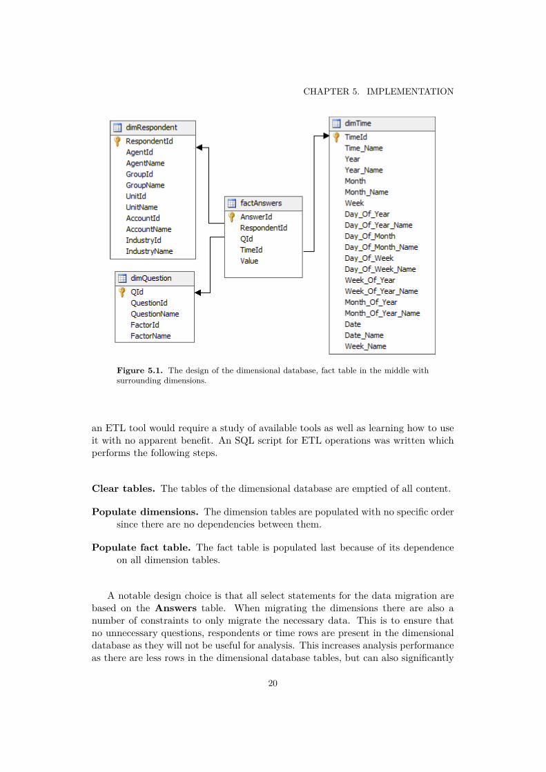
The dimensional database will consist of one fact table holding the quantified valuesfrom given answers. The fact table includes foreign keys to each of the dimensiontables which provides information to the answer. In this case there were three fun-damental questions that needed to be answered in order to be able to analyze thedata; who, what and when. These three questions are answered by the Respon-dent, Question and Time dimensions respectively and will be explained in thefollowing three sections. Section 5.1.2.4 will explain the design of the Answers facttable which connects the dimensions. Figure 5.1 illustrates the resulting tables andtheir relations in the dimensional database.
All attributes in a dimension will have a key value to identify it. For presen-tation to the user this key value may not be intuitive enough, and thus a match-ing Name column is created for most columns. For example, the Day_Of_Weekcolumn has an integer value between 1 and 7 and has a matching name columnDay_Of_Week_Name with a value of "Monday" to "Sunday" instead.
5.1.2.1 Respondent dimension
The Respondent dimension is designed to answer the questionwho, and its most finegrained member is the respondent. In this case, the respondent defines a respondentof a single survey. Even if the same person responds to several surveys, they willbe stored as a different respondent each time. This has the immediate consequencethat every answer from a single respondent also comes from the same survey whichenables analysis on the level of individual surveys.
Each respondent is part of a hierarchy defined as Industry → Account1 →Unit→ Group→ Agent→ Respondent.
5.1.2.2 Question dimension
The Question dimension is designed to answer the question what, and its most finegrained member is the question. A question can, for instance, be "How satisfiedare you in general with our services?". Each question is a child to a parent factorwhich may for instance be "General satisfaction". Each factor can have severaloften similar child questions. In some cases a question can have several factors inthe source database resulting in one separate question is created for each factorin the dimensional database. This also means that a QuestionId is not alwaysunique making it necessary to use a separate, generated QId as a primary key. Thisdimension has one short hierarchy of Factor → Question.
1An "account" is a company. The name "account" is chosen for consistency with the sourcedata.
18
5.1. DATABASE CONVERSION
5.1.2.3 Time dimension
The Time dimension is designed to answer the question when, and its most finegrained member is the time with an hour precision. The source data enables amuch higher precision, but in this case an hour precision is sufficient. Using thislower precision allows for a smaller Time table resulting in improved performance.Each hour is part of the natural hierarchies Y ear → Month→ Date→ Time andY ear → Week → Date → Time, where both are useful for the web interface aswell as analysis.
In excess of the values necessary to create these two hierarchies a number ofother values are included as well for other kinds of analysis.
Day_Of_Year Day number of current year.Day_Of_Month Day number of current month.Day_Of_Week Day number of current week.Week_Of_Year Week number of current year.Month_Of_Year Month number of current year.
These values can be used to filter the data in order to answer questions such as "Arecustomers generally more satisfied on Fridays than Mondays?" and "Does customersof company X generally feel the response time is higher during these months?".
5.1.2.4 Answers fact table
One row in the Answers fact table corresponds to an answer to a single question,resulting in a value from 1 to 5 if it’s a numeric question or 1 or 5 if it’s a yes/noquestion. In excess of this number each row in the fact table also includes a referenceto one row in each of the three dimensions.
5.1.3 ETL operations
ETL operations were used to extract the relevant data from the OLTP databaseused by Bright to the new dimensional database schema. Data that was not deemeduseful for analysis purposes were filtered out, such as answers that does not followthe numeric or yes/no format and respondents that have no answers connected tothem. Redundant data was added where deemed necessary, most prominently thetime dimension in which all columns are derived from the submission time of thesurvey (see section 5.1.2.3).
Since both the data source and destination were on SQL Servers, the simplestsolution for ETL operations was to write an SQL script. The alternative of using
19
CHAPTER 5. IMPLEMENTATION
Figure 5.1. The design of the dimensional database, fact table in the middle withsurrounding dimensions.
an ETL tool would require a study of available tools as well as learning how to useit with no apparent benefit. An SQL script for ETL operations was written whichperforms the following steps.
Clear tables. The tables of the dimensional database are emptied of all content.
Populate dimensions. The dimension tables are populated with no specific ordersince there are no dependencies between them.
Populate fact table. The fact table is populated last because of its dependenceon all dimension tables.
A notable design choice is that all select statements for the data migration arebased on the Answers table. When migrating the dimensions there are also anumber of constraints to only migrate the necessary data. This is to ensure thatno unnecessary questions, respondents or time rows are present in the dimensionaldatabase as they will not be useful for analysis. This increases analysis performanceas there are less rows in the dimensional database tables, but can also significantly
20
5.2. DATA CUBE IMPLEMENTATION
increase the time to perform ETL operations because of more complexity in theETL script. This is analyzed further in chapter 6.
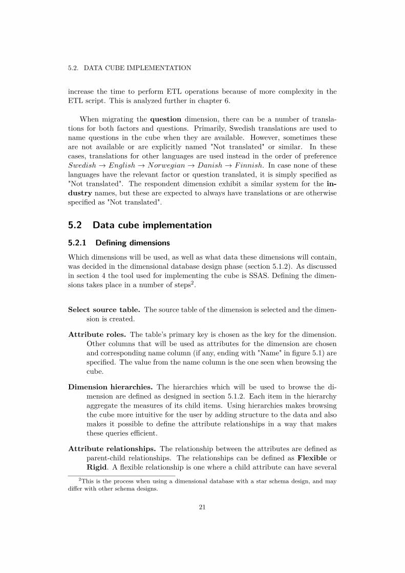
When migrating the question dimension, there can be a number of transla-tions for both factors and questions. Primarily, Swedish translations are used toname questions in the cube when they are available. However, sometimes theseare not available or are explicitly named "Not translated" or similar. In thesecases, translations for other languages are used instead in the order of preferenceSwedish → English → Norwegian → Danish → Finnish. In case none of theselanguages have the relevant factor or question translated, it is simply specified as"Not translated". The respondent dimension exhibit a similar system for the in-dustry names, but these are expected to always have translations or are otherwisespecified as "Not translated".
5.2 Data cube implementation
5.2.1 Defining dimensionsWhich dimensions will be used, as well as what data these dimensions will contain,was decided in the dimensional database design phase (section 5.1.2). As discussedin section 4 the tool used for implementing the cube is SSAS. Defining the dimen-sions takes place in a number of steps2.
Select source table. The source table of the dimension is selected and the dimen-sion is created.
Attribute roles. The table’s primary key is chosen as the key for the dimension.Other columns that will be used as attributes for the dimension are chosenand corresponding name column (if any, ending with "Name" in figure 5.1) arespecified. The value from the name column is the one seen when browsing thecube.
Dimension hierarchies. The hierarchies which will be used to browse the di-mension are defined as designed in section 5.1.2. Each item in the hierarchyaggregate the measures of its child items. Using hierarchies makes browsingthe cube more intuitive for the user by adding structure to the data and alsomakes it possible to define the attribute relationships in a way that makesthese queries efficient.
Attribute relationships. The relationship between the attributes are defined asparent-child relationships. The relationships can be defined as Flexible orRigid. A flexible relationship is one where a child attribute can have several
2This is the process when using a dimensional database with a star schema design, and maydiffer with other schema designs.
21
CHAPTER 5. IMPLEMENTATION
parent attributes. For example, a question has a flexible relationship to afactor. This is because the same question can have several factors. A rigidrelationship is one where a child attribute only have one parent attribute. Forexample, a month has a rigid relationship to a year - the month May 2013 willalways relate to the year 2013. A rigid relationship may be defined as a flexibleone without errors, but the reverse is not true. Choosing the correct attributerelationship is important to avoid incorrect computations and optimize queryand processing performance[21].
Subsections 5.2.1.1 through 5.2.1.3 will briefly describe these steps for each ofthe dimensions. In the attribute relationship figures arrows are used to denoteattribute relationships. A filled arrow means a relationship is rigid and a hollowarrow means it’s flexible.
5.2.1.1 Respondent dimension
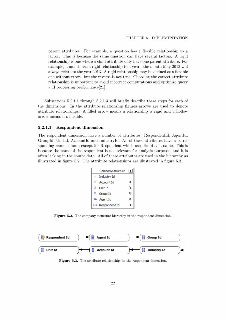
The respondent dimension have a number of attributes: RespondentId, AgentId,GroupId, UnitId, AccountId and IndustryId. All of these attributes have a corre-sponding name column except for Respondent which uses its Id as a name. This isbecause the name of the respondent is not relevant for analysis purposes, and it isoften lacking in the source data. All of these attributes are used in the hierarchy asillustrated in figure 5.2. The attribute relationships are illustrated in figure 5.3.
Figure 5.2. The company structure hierarchy in the respondent dimension.
Figure 5.3. The attribute relationships in the respondent dimension.
22

5.2. DATA CUBE IMPLEMENTATION
5.2.1.2 Question dimension
The question dimension only have three attributes: QId, QuestionId and FactorId.QuestionId and FactorId have corresponding name columns and are used in thehierarchy as illustrated in figure 5.4. The attribute relationships are illustrated infigure 5.5.
Figure 5.4. The question hierarchy in its dimension.
Figure 5.5. The attribute relationships in the question dimension.
5.2.1.3 Time dimension
The weeks follow the ISO 8601 standard of week enumeration because ISO weeknumbers are unique per year[22]. This allows for a rigid relationship between yearand week. The two hierarchies of the time dimension are illustrated in figure 5.6.The attribute relationships are illustrated in figure 5.7.
Figure 5.6. The Y ear → Month → Date → T ime and Y ear → W eek → Date →T ime hierarchies in the time dimension.
5.2.2 Creating the cubeThe cube was created by selecting the fact table and choosing the measures thatshould be included from it. All three connected dimensions are then chosen so thecube can be browsed using them. In SSAS there are some standard measures thatcan be used whereof three were used in this prototype.
23

CHAPTER 5. IMPLEMENTATION
Figure 5.7. The attribute relationships in the time dimension. The attributes listedbelow TimeId have a flexible relationship to TimeId, but are not part of a hierarchy.
Sum. Aggregates the sum of all children values. Used to calculate the averagevalue.
Non-empty count. Aggregates the number of non-empty data points found. Aregular count does not work because respondents do not always answer allquestions, and thus different questions need different counts.
Distinct count. Aggregates the number of distinct items. In this case, the numberof distinct respondents.
After these base measures and all the dimensions are chosen, calculated memberscan be added where the formulas that calculate the member are written by thedeveloper. The only calculated member necessary in this prototype is the average,calculated as the sum divided by the non-empty count.[23]
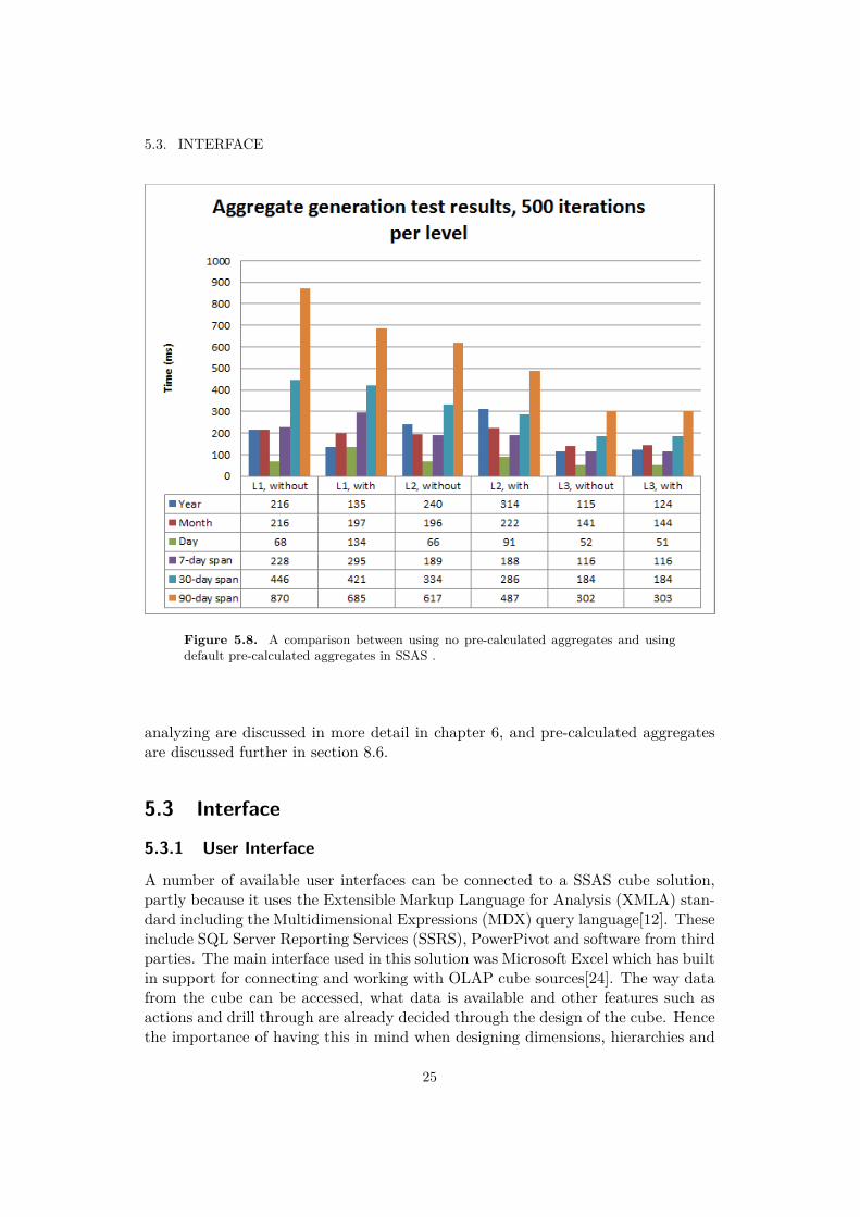
By default, no pre-calculated aggregations are used. Default pre-calculated ag-gregations can be set for the measure groups to let SSAS choose the optimal ag-gregates to pre-calculate based on the data set. By testing the solution both withand without these pre-calculated aggregates, a number of differences are noticed.The reader is referred to figure 5.8 for a chart over the performance difference. Thetest is run for all three levels, whereas a "level" refers to a level in the organizationhierarchies (abbreviated "Ln" where n is the level number). 500 different date/orga-nization sets each level, and the time required averaged. Averaging these averages,it turns out that the average time required is 255 ms without the pre-calculatedaggregates and 243 ms with them - a performance increase of as little as 4.9%. Thisis not necessarily because pre-calculated aggregates are not efficient, but rather thatthe default aggregates are not fit to the way the cube is used. In addition to theperformance difference, the cube takes 1866 MB as opposed to 759 MB withoutthe pre-calculated aggregates, and takes 11:06 minutes instead of 07:08 minutes toprocess. Because of the minimal performance gain (<5%) and costs in space andprocessing, no pre-calculated aggregates were used. The methods of testing and
24
5.3. INTERFACE
Figure 5.8. A comparison between using no pre-calculated aggregates and usingdefault pre-calculated aggregates in SSAS .
analyzing are discussed in more detail in chapter 6, and pre-calculated aggregatesare discussed further in section 8.6.
5.3 Interface
5.3.1 User Interface
A number of available user interfaces can be connected to a SSAS cube solution,partly because it uses the Extensible Markup Language for Analysis (XMLA) stan-dard including the Multidimensional Expressions (MDX) query language[12]. Theseinclude SQL Server Reporting Services (SSRS), PowerPivot and software from thirdparties. The main interface used in this solution was Microsoft Excel which has builtin support for connecting and working with OLAP cube sources[24]. The way datafrom the cube can be accessed, what data is available and other features such asactions and drill through are already decided through the design of the cube. Hencethe importance of having this in mind when designing dimensions, hierarchies and
25

CHAPTER 5. IMPLEMENTATION
measures in the cube.
The goal of this implementation has been to provide a way to group data belong-ing to a single respondent and list the given answers by question. This is achievedby using pivot tables in Excel. The respondent hierarchy is used for the rows, thequestion hierarchy is used for the columns and the data is filtered using the time di-mension. Lastly the desired measures are added to the pivot table, being displayedfor each cell that has a value. An example of the result can be seen in figures 5.9and 5.103.
5.3.2 Application InterfaceIn order to allow other applications such as the web interface to access values in thecube in a convenient way, an Application Programming Interface (API) is needed.When browsing the cube through a Graphical User Interface (GUI) such as Excel,what actually happens is that Excel generates appropriate MDX statements, queriesthe OLAP server and presents the returned result. The used MDX queries can beidentified by using the SQL Server Profiler[25]. Similarly, MDX queries can be usedin applications to access the SSAS cube.
3The data presented in the examples have had confidential information changed.
26

5.3. INTERFACE
Figure 5.9. An example of coarser aggregated cube values as viewed in Excel.
Figure 5.10. An example of a detailed view of individual respondents as viewed inExcel.
27


Chapter 6
Analysis
The analysis phase of this degree project was divided into two parts; aggregatesand correlational analysis. The reason for this distinction is that the calculationof aggregates is fully implemented and can be accessed using an API in both thecurrent solution and the solution developed for this degree project, and thus it canbe tested and compared programmatically. The correlational analysis on the otherhand is in the current solution subject to a significant amount of manual processingand less so in the solution developed for this degree project. For that reason it isnot feasible to test the difference programmatically, but the difference will ratherbe analyzed in discussion with Bright’s analysts.
6.1 Aggregate analysis
In order to analyze the difference between the current solution and the solutionimplemented for this degree project in terms of aggregates, C# Test Units wereused. The tests attempts to answer the questions of the implemented solutionvalidity (i.e. if the generated answers are correct) and performance (i.e. how muchfaster or slower the solution is) compared to the current solution.
The tests are adapted to provide a meaningful comparison between the currentsolution and the developed prototype. The web interface allows the user to selecta company, unit, group or agent in a hierarchy as well as a time span ranging overthe previous and current year. The web interface then provides the user with theanswer average from respondents on a set of factors for the chosen entity company,unit, group or agent as well as a comparison to the corresponding upper level inthe hierarchy. For example, choosing a group would give a comparison to thecorresponding unit. The tests of both the current solution and prototype providesthe same comparison.
Measurements are taken for a random time interval in each of six categories; A
29
CHAPTER 6. ANALYSIS
full year (such as 2012), month (such as May 2012), day (such as 2012-07-13) as wellas randomly chosen time spans of 7, 30 and 90 days respectively. The reason forhaving both full years, months and days as well as random time spans is to analyzehow the prototype performance differs from random spans to possibly pre-aggregatesvalues in the defined hierarchies. While a full month such as 2012 − 06 − 01 →2012−06−31 is reasonably performance-wise equal to 2012−06−08→ 2012−07−07in the current solution, the prototype might exhibit different performance.
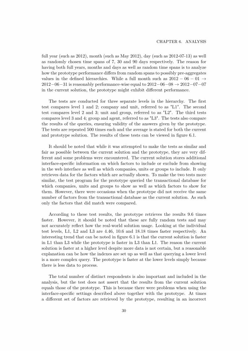
The tests are conducted for three separate levels in the hierarchy. The firsttest compares level 1 and 2; company and unit, referred to as "L1". The secondtest compares level 2 and 3; unit and group, referred to as "L2". The third testscompares level 3 and 4; group and agent, referred to as "L3". The tests also comparethe results of the queries, ensuring validity of the answers given by the prototype.The tests are repeated 500 times each and the average is stated for both the currentand prototype solution. The results of these tests can be viewed in figure 6.1.
It should be noted that while it was attempted to make the tests as similar andfair as possible between the current solution and the prototype, they are very dif-ferent and some problems were encountered. The current solution stores additionalinterface-specific information on which factors to include or exclude from showingin the web interface as well as which companies, units or groups to include. It onlyretrieves data for the factors which are actually shown. To make the two tests moresimilar, the test program for the prototype queried the transactional database forwhich companies, units and groups to show as well as which factors to show forthem. However, there were occasions when the prototype did not receive the samenumber of factors from the transactional database as the current solution. As suchonly the factors that did match were compared.
According to these test results, the prototype retrieves the results 9.6 timesfaster. However, it should be noted that these are fully random tests and maynot accurately reflect how the real-world solution usage. Looking at the individualtest levels, L1, L2 and L3 are 4.46, 10.6 and 18.18 times faster respectively. Aninteresting trend that can be noted in figure 6.1 is that the current solution is fasterin L1 than L3 while the prototype is faster in L3 than L1. The reason the currentsolution is faster at a higher level despite more data is not certain, but a reasonableexplanation can be how the indexes are set up as well as that querying a lower levelis a more complex query. The prototype is faster at the lower levels simply becausethere is less data to process.
The total number of distinct respondents is also important and included in theanalysis, but the test does not assert that the results from the current solutionequals those of the prototype. This is because there were problems when using theinterface-specific settings described above together with the prototype. At timesa different set of factors are retrieved by the prototype, resulting in an incorrect
30

6.2. CORRELATIONAL ANALYSIS
Figure 6.1. Test of average factor retrieval times comparing current solution andprototype for all three test levels.
distinct respondent count. Despite of this, in the random tests conducted, thecorrect number of distinct respondents was retrieved in 96% of the tests.
Furthermore, because it is possible for rounding errors to occur during the dif-ferent processing stages, factor accuracy is only asserted within a 10−9 error margin.During the tests, all compared factor results were consistent between the currentsolution and the prototype.
6.2 Correlational analysisIn the current solution, as discussed in chapter 2, there is no reasonable way to ex-tract information in a format that allows correlational analysis. This has restricted
31

CHAPTER 6. ANALYSIS
analysis to be made primarily on aggregates which proves less valuable than if it isdone on individual data. The prototype opens up possibilities to generate reportsbased on correlational analysis in a flexible and convenient way by presenting theinformation in a useful format in Excel (see figure 5.10).
Figure 6.2. Chart over the correlation calculation time for different number of rows.Note that both axises are exponential. The retrieved number of rows are not exactlyas stated, but chosen to be as close as possible.
Once data is retrieved in a usable format in Excel, adding the formulas foranalysis calculations is simple and straightforward for users experienced with Excel.Depending on the number of rows involved in the calculations, retrieval can takesignificant time. In order to assess the performance of correlational analysis, atypical test case was set up and tested for different number of rows. Each row inthe test is an individual respondent. The test case aims to calculate the correlationbetween two often used factors. For retrieving a smaller number of rows, a shorttime span for a single agent, group or unit is used. For a large number of rows, along time span for an industry or a company is used. Refer to figure 6.2 for the testresults.
Most of the correlational analysis done by Bright’s analysts is focused on specificgroups in organizations and specific time spans, and thus the number of rows beingused are generally not excessively high. In these cases, correlational analysis ishighly responsive with times below 2 seconds. In the rare cases that the number ofrows used exceeds 10,000, the calculation delays will be noticeable but well withinacceptable boundaries. As of Excel 2010, correlational analysis is limited to 220 =
32
6.3. ETL OPERATIONS AND CUBE PROCESSING
1, 048, 576 rows[26].
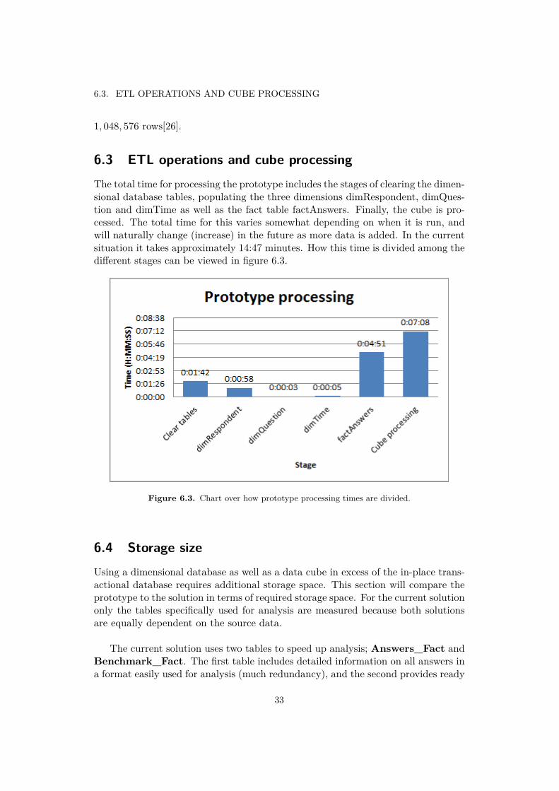
6.3 ETL operations and cube processingThe total time for processing the prototype includes the stages of clearing the dimen-sional database tables, populating the three dimensions dimRespondent, dimQues-tion and dimTime as well as the fact table factAnswers. Finally, the cube is pro-cessed. The total time for this varies somewhat depending on when it is run, andwill naturally change (increase) in the future as more data is added. In the currentsituation it takes approximately 14:47 minutes. How this time is divided among thedifferent stages can be viewed in figure 6.3.
Figure 6.3. Chart over how prototype processing times are divided.
6.4 Storage sizeUsing a dimensional database as well as a data cube in excess of the in-place trans-actional database requires additional storage space. This section will compare theprototype to the solution in terms of required storage space. For the current solutiononly the tables specifically used for analysis are measured because both solutionsare equally dependent on the source data.
The current solution uses two tables to speed up analysis; Answers_Fact andBenchmark_Fact. The first table includes detailed information on all answers ina format easily used for analysis (much redundancy), and the second provides ready
33

CHAPTER 6. ANALYSIS
numbers for different factors for all industries. These tables take up 15,091,816 KBand 600 KB respectively, adding up to 15,092,416 KB or approximately 14.39 GB.Most of this space, approximately two thirds, are indexes used for speeding upqueries.
The prototype uses both the dimensional database and a data cube for analysis.The dimensional database is made up of four tables; the three dimensions dimRe-spondent, dimQuestion and dimTime as well as the fact table factAnswers. Thesetables take up 459,408 KB, 240 KB, 9,232 KB and 654,992 KB respectively. Thedata cube takes up approximately 759.92 MB. In total, this adds up to approxi-mately 1.81 GB.
34
Chapter 7
Conclusions
The developed prototype consistently delivers correct results in an efficient manner.According to the tests in chapter 6, analysis performance is improved severalfold. Itdoes so using significantly less storage space than the current solution, and is keptup-to-date using nightly procedures well within acceptable boundaries in terms ofprocessing times. Because all analysis is done on the data warehouse solution,customer use of the transactional database is not adversely affected beyond thenightly procedures.
In addition to improving performance, the prototype allows for flexible dataextraction making new kinds of analysis possible. This allows Bright to offer newservices to their customers that they do desire, but have previously been restrictedfrom implementing because the current solution was never intended for such flexi-bility.
Looking back at the choice of method made in chapter 4, using OLAP softwarespecialized in data analysis and choosing SSAS over one of the alternative toolssuch as Palo, Jedox or Oracle Essbase turned out to be a good choice leading toa well-functional result that was possible to develop within the given time frame.Because there has not been an equal amount of time spent on each of the candidatetools we cannot determine if we made the optimal choice, but only that it sufficed.
One of the major features of an OLAP cube that made us turn to such a so-lution was the possibility of having pre-calculated aggregates that could speed upanalysis significantly. As it turns out, we ended up not implementing pre-calculatedaggregates in the prototype as the performance gains were minimal as discussed insection 5.2.2. The structure of the cube make analysis efficient enough even withoutthose pre-calculated aggregates.
The prototype is only intended as a prototype and as such lacks some of thefeatures needed for it to be implemented in a production environment, as discussedin section 1.3. Possible future developments of the prototype are discussed in chapter8 dedicated to this subject.
35


Chapter 8
Recommendations
This chapter will discuss possible future developments for the solution, organizedinto separate sections.
8.1 Selective ETL
In the current solution the ETL script simply clears the dimensional database andre-copies everything from the OLTP. This is a simple solution that works well fornow considering that the total ETL time is less than 10 minutes and is done nightly.However, if the database continues to grow rapidly the ETL time may become un-acceptably long. Furthermore, the current dimensional database is implemented asits own schema in the OLTP database allowing high transfer speeds. In case the di-mensional database was to be moved to a different server in a different location, thismeans that network transfer speeds could bottleneck the ETL operations resultingin more time needed to perform the nightly ETL.
It is recommended that a selective ETL solution is developed to only copy thechanged data if these conditions are to change. This would significantly lower thetime required for ETL and ensure that it is not overwhelmed by future databasesizes and slower network connectivity.
8.2 Real-time synchronization
In the current solution the ETL script is only run nightly, and section 8.1 suggestsa more optimal means to the same end. A different approach would be to havethe OLTP database update the dimensional database every time a change is made,allowing for real-time analysis. This approach, however, has implications for thecube as different sections would have to be reprocessed as well. There are a numberof approaches to address this issue.
37

CHAPTER 8. RECOMMENDATIONS
• It is possible to use an incremental process in SSAS to only process changedvalues. This approach may introduce significant processing overhead.
• Another alternative is to use the ROLAP storage mode in SSAS for real-time analysis. ROLAP stands for Relational Online Analytical Processing,and in short means that both atomic data and aggregations are stored in therelational database. This approach would allow for real-time analysis, butmay also decrease performance significantly because the relational databaseis not optimized for large queries.
• The cube is currently using the MOLAP storage mode. MOLAP stands forMultidimensional Online Analytical Processing and means that both atomicdata and aggregations are stored in a highly optimized format in the cube.It is possible to use this storage mode for historical data and correspondingqueries, and use the ROLAP storage mode for a small partition for real-timequeries.
The third option is most likely to be the optimal solution, but more research aroundthe are is required to make an informed decision on which approach to choose.
8.3 Redundant questions
Because the questions in the Bright database are indirectly administrated by manythird parties, and there is a common need to ask approximately the same questions(e.g. "Are you generally satisfied with our customer support?"), it has come tobeing many identical or similar questions in the transactional database. Whilethis doesn’t have any direct consequences, it could certainly complicate analysis asanswers to "basically the same question" are scattered across several questions. Thiscould be improved by implementing fuzzy logic in the ETL solution to remove suchredundancy.
This may however not be a relevant problem. Multiple similar questions aremost likely part of the same factor on which the analysis could equally well bemade. Implementing fuzzy logic to help reduce this redundancy could also presentnew problems if the fuzzy logic makes mistakes.
8.4 Web interface using the cube
As of now the web interface still uses the transactional database to generate theaggregate data that’s presented to the users. The web interface could use thecube instead to reap the benefits of increased performance as well as not disrupttransactions done on the transactional database.
38

8.5. MOVE DATA WAREHOUSE TO SPECIFIC DATABASE
Because the web interface has several interface-specific settings defining whichinformation to show for specific companies, units and groups, the cube must bemodified to fit those needs. One approach would be to tailor the cube to the needs ofthe web interface, but this could have negative implications in terms to analysis andincrease cube complexity significantly. A preferable approach would be implement alayer between the web interface and the cube that handles interface-specific settings.This middle layer could simply query the transactional database where these settingsare stored (such queries are trivial in comparison to calculating aggregates) and usethem to extract only the necessary information from the cube using OLAP queries.By getting interface-specific information from the transactional database, changesin the interface (made by users) can be made in real-time even if the cube is notprocessed as such.
The main problem of this approach is that queries can be made for the currentday, for which the OLAP cube does not have information. Because real-time in-formation is important in the web interface, disabling this feature is not an option.There are two distinct approaches to this problem. The first approach is to updatethe cube in real-time as discussed in section 8.2 allowing the cube to fully replacethe current solution. The second approach is to combine the cube with the currentsolution, retrieving historical data from the cube and the current day’s data fromthe current solution.
8.5 Move data warehouse to specific database
The data warehouse is currently hosted on the same database as the transactionaldatabase, only under a different schema. In production, this could be hosted ona different server in order to completely separate the OLTP and OLAP solutions.This would be an interesting option if the analysis is using up considerable resourcesfrom the shared server, adversely affecting the use of the transactional database.
8.6 Optimize cube pre-calculated aggregates
The cube in SSAS is currently not using any pre-calculated aggregates. As discussedin chapter 6, the performance in the prototype is greatly increased as compared tothe previous solution. However, the performance might be possible to increasesignificantly by optimizing the choices of which aggregates to include as well as thestructure of these.
The optimal configuration of this is highly dependent on the usage of the cubeand requires co-operation with the end users of the cube. If the necessary researchon cube usage is made, informed decisions on which aggregates to include and howto partition them can be made and better performance achieved.
39

CHAPTER 8. RECOMMENDATIONS
8.7 Server side correlational calculationsIn the developed solution, it is easy to extract information in a highly flexible andefficient manner that is useful for correlational analysis. Selecting which rows toshow in Excel with which columns allows the user (assumed familiar with Excel syn-tax) to simply use Excel syntax to calculate different things. However, with a hugeamount of rows in the magnitudes of tens or hundreds of thousands, this becomes apoorly responsive approach because huge amounts of data needs to be transferredand stored in an Excel spreadsheet. This is an issue that can be addressed by re-moving the need to view the individual rows and instead do the calculations on theserver side, delivering only the sought answer to the user.
One option to achieve this is to use the built-in data mining available in SSAS.This option would allow further automation of correlational analysis done com-pletely on the server side.[27]
40
References
[1] Gartner Says Worldwide Business Intelligence Software Revenue to Grow 7Percent in 2013, Rob van der Meulen and Janessa Rivera, 2013-02-19, http://www.gartner.com/newsroom/id/2340216, Retrieved 2013-04-15
[2] Business Intelligence (BI), Gartner IT Glossary, http://www.gartner.com/it-glossary/business-intelligence-bi/, Retrieved 2013-04-18
[3] Data Warehousing Concepts, Oracle Documentation, http://docs.oracle.com/cd/B10500_01/server.920/a96520/concept.htm, Retrieved 2013-04-18
[4] Data Warehouse, Gartner IT Glossary, http://www.gartner.com/it-glossary/data-warehouse/, Retrieved 2013-04-18
[5] What is big data?, IBM, http://www-01.ibm.com/software/data/bigdata/,Retrieved 2013-04-18
[6] What is Data Mining?, Oracle Documentation, http://docs.oracle.com/cd/B28359_01/datamine.111/b28129/process.htm, Retrieved 2013-04-15
[7] SQL Server 2005 Analysis Services - Step by Step, Reed Jacobson and StaciaMisner, 2006, Hitachi Consulting
[8] Oracle Business Intelligence Tools and Technology, Oracle, http://www.oracle.com/us/solutions/business-analytics/business-intelligence/overview/index.html, Retrieved 2013-05-01
[9] Essbase Studio User Guide, Oracle, 2012-08, http://docs.oracle.com/cd/E38445_01/doc.11122/est_user.pdf, Retrieved 2013-04-26
[10] Oracle Hyperion Smart View for Office User Guide, Oracle, 2013-03, http://docs.oracle.com/cd/E38438_01/epm.111223/sv_user.pdf, Retrieved 2013-04-26
[11] Essbase MDX Queries, Oracle Documentation, http://docs.oracle.com/cd/E10530_01/doc/epm.931/html_esb_dbag/frameset.htm?dmaxldml.htm, Re-trieved 2013-05-21
41
REFERENCES
[12] SSAS 2008 R2 - Technical Reference, Microsoft Documentation, http://technet.microsoft.com/en-us/library/bb500210(v=sql.105).aspx,Retrieved 2013-04-30
[13] First Steps with Jedox for Excel version 5.0, Jedox Documenta-tion http://www.jedox.com/en/jedox-downloads/documentation/5/first-steps-with-jedox-for-excel-5-manual.html, Retrieved 2013-04-26
[14] Jedox ETL Server Manual version 4.0, Jedox Documenta-tion, http://www.jedox.com/en/jedox-downloads/documentation/jedox-etl-server-4-manual.html, Retrieved 2013-04-26
[15] First Steps with Jedox Web version 5.0, Jedox Documentationhttp://www.jedox.com/en/jedox-downloads/documentation/5/first-steps-with-jedox-web-5-manual.html, Retrieved 2013-05-21
[16] Jedox 3rd Party Software, Jedox Documentation, http://www.jedox.com/en/jedox-downloads/documentation/5/jedox-3rd-party-software-5-manual.html, Retrieved 2013-05-21
[17] Creating a PowerPivot Workbook on SharePoint, Microsoft Documentation,http://technet.microsoft.com/en-us/library/gg413412.aspx, Retrieved2013-05-22
[18] PowerPivot capacity specification, Microsoft Documentation, http://technet.microsoft.com/en-us/library/gg413465.aspx, Retrieved 2013-05-22
[19] Software boundaries and limits for SharePoint 2013, Microsoft Documenta-tion, http://technet.microsoft.com/en-us/library/cc262787.aspx, Re-trieved 2013-05-22
[20] PowerPivot Features, Microsoft Documentation, http://msdn.microsoft.com/en-us/library/ee210639(v=sql.105).aspx, Retrieved 2013-05-22
[21] Configure Attribute Relationship Properties, Microsoft Documentation, http://msdn.microsoft.com/en-us/library/ms176124.aspx, Retrieved 2013-04-29
[22] A summary of the international standard date and time notation, MarkusKuhn, http://www.cl.cam.ac.uk/~mgk25/iso-time.html, Retrieved 2013-04-29
[23] Defining Calculated Members, Microsoft Documentation, http://msdn.microsoft.com/en-us/library/ms166568.aspx, Retrieved 2013-04-30
42
REFERENCES
[24] Microsoft Office OLAP overview, Microsoft Documenta-tion, http://office.microsoft.com/en-001/excel-help/overview-of-online-analytical-processing-olap-HP010177437.aspx,Retrieved 2013-04-30
[25] Monitoring Analysis Services with SQL Server Profiler, Microsoft Documen-tation, http://msdn.microsoft.com/en-us/library/ms174779.aspx, Re-trieved 2013-05-03
[26] Excel specifications and limits, Microsoft Documenta-tion, http://office.microsoft.com/en-us/excel-help/excel-specifications-and-limits-HP010073849.aspx, Retrieved 2013-04-15
[27] Data Mining in SSAS, Microsoft Documentation, http://msdn.microsoft.com/en-us/library/bb510516.aspx, Retrieved 2013-05-14
43