Flexible-Cost SLAM

by

Matthew Koichi Grimes

A dissertation submitted in partial fulfillment

of the requirements for the degree of

Doctor of Philosophy

Department of Computer Science

New York University

May 2012

Professor Yann LeCun

c© Matthew Koichi Grimes

All Rights Reserved, 2012

For Lyubashka.

iii

Acknowledgements

My parents come first in this list of thanks, for their support. My friend Yotam

comes second, for his example.

Thanks to my history of professors, who have channeled my progress: Nancy

Pollard, Greg Turk, Aaron Bobick, Jovan Popovic, Takeo Igarashi, and finally,

Yann.

This thesis was written in a nomadic state across three cites and two coasts.

Thank you to Gail Baugh and Jim Warshell for their opening their home to me

in San Francisco. Thanks to the cafes Diesel and TrueGrounds, the Tisch Library

at Tufts, and the Physics Reading Room at MIT, for providing a daily desk to a

stranger. Thanks to Flying Lotus for the soundtrack, and Lenovo for a long-lasting

battery.

While not a professor, no person has helped me more with the nuts and bolts

of writing code than Drago Anguelov of Google, whose perfectionism and generous

contributions of data went well above the call of duty of an ex-boss. This thesis,

and my work in general, has benefitted immeasurably.

Finally, thank you to my wife Lyuba, with whom all is possible.

iv

Abstract

The ability of a robot to track its position and its surroundings is critical in

mobile robotics applications, such as autonomous transport, farming, search-and-

rescue, and planetary exploration.

As a foundational building block to such tasks, localization must remain reliable

and unobtrusive. For example, it must not provide an unneeded level of precision,

when the cost of doing so displaces higher-level tasks from a busy CPU. Nor should

it produce noisy estimates on the cheap, when there are CPU cycles to spare.

This thesis explores localization solutions that provide exactly the amount of

accuracy needed to a given task. We begin with a real-world system used in the

DARPA Learning Applied to Ground Robotics (LAGR) competition. Using a

novel hybrid of wheel and visual odometry, we cut the cost of visual odometry

from 100% of a CPU to 5%, clearing room for other critical visual processes, such

as long-range terrain classification. We present our hybrid odometer in chapter 2.

Next, we describe a novel SLAM algorithm that provides a means to choose the

desired balance between cost and accuracy. At its fastest setting, our algorithm

converges faster than previous stochastic SLAM solvers, while maintaining signifi-

v

cantly better accuracy. At its most accurate, it provides the same solution as exact

SLAM solvers. Its main feature, however, is the ability to flexibly choose any point

between these two extremes of speed and precision, as circumstances demand. As

a result, we are able to guarantee real-time performance at each timestep on city-

scale maps with large loops. We present this solver in chapter 3, along with results

from both commonly available datasets and Google Street View data.

Taken as a whole, this thesis recognizes that precision and efficiency can be

competing values, whose proper balance depends on the application and its fluc-

tuating circumstances. It demonstrates how a localizer can and should fit its cost

to the task at hand, rather than the other way around. In enabling this flexibil-

ity, we demonstrate a new direction for SLAM research, as well as provide a new

convenience for end-users, who may wish to map the world without stopping it.

vi

Contents

Dedication . . . . . . . . . . . . . . . . . . . . . . . . . . . . . . . . . iii

Acknowledgements . . . . . . . . . . . . . . . . . . . . . . . . . . . . iv

Abstract . . . . . . . . . . . . . . . . . . . . . . . . . . . . . . . . . . v

List of Appendices . . . . . . . . . . . . . . . . . . . . . . . . . . . . ix

List of Figures . . . . . . . . . . . . . . . . . . . . . . . . . . . . . . . xvi

List of Tables . . . . . . . . . . . . . . . . . . . . . . . . . . . . . . . xvii

1 Introduction 1

2 Efficient Off-Road Localization with Visually Corrected Odom-

etry 5

2.1 Introduction . . . . . . . . . . . . . . . . . . . . . . . . . . . . . 6

2.2 Related Work . . . . . . . . . . . . . . . . . . . . . . . . . . . . 8

2.3 Algorithm . . . . . . . . . . . . . . . . . . . . . . . . . . . . . . 11

2.4 Implementation . . . . . . . . . . . . . . . . . . . . . . . . . . . 18

2.5 Results . . . . . . . . . . . . . . . . . . . . . . . . . . . . . . . . 19

2.6 Conclusions and Future Work . . . . . . . . . . . . . . . . . . . 21

vii

3 Hybrid Hessians for SLAM with Tunable Cost and Accuracy 25

3.1 Introduction . . . . . . . . . . . . . . . . . . . . . . . . . . . . . 26

3.2 Related Work . . . . . . . . . . . . . . . . . . . . . . . . . . . . 28

3.3 Algorithm . . . . . . . . . . . . . . . . . . . . . . . . . . . . . . 31

3.4 Results . . . . . . . . . . . . . . . . . . . . . . . . . . . . . . . . 53

3.5 Conclusions and Future Work . . . . . . . . . . . . . . . . . . . 57

4 Conclusions and Future Work 67

Bibliography 95

viii

List of Appendices

A Differentiating Hierarchical Poses 70

B Constraint Jacobians 83

ix

List of Figures

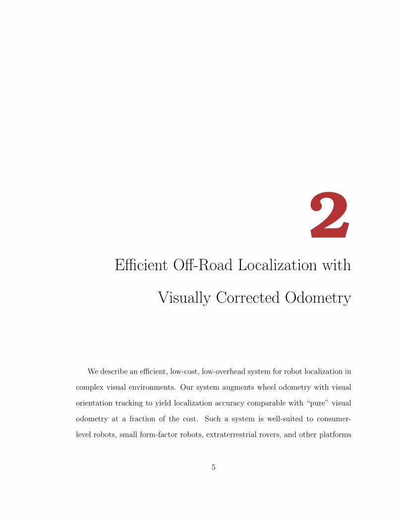
2.1 A rectified camera image and its spherical transform. The asymmetry of

the spherical image is due to the fact that the camera is pointed off to

the left and down, with some axial roll. The robot is pointed straight at

the area highlighted by four yellow dots, placed at pitch and yaw values

[0.03, 0.1], [0.03,−0.1], [−0.03,−0.1], and [−0.03, 0.1], in radians. After

the transformation, these points form an axis-aligned rectangle around

the frontal direction. In practice, we transform only the portion of the

camera image roughly located around the horizon, highlighted by the

green rectangle above. . . . . . . . . . . . . . . . . . . . . . . . . 12

x

2.2 Parallax from pure forward motion. We wish to limit our atten-

tion to objects which will not shift under parallax from frame to frame.

In a spherical image where each pixel subtends θp radians of yaw, this

requires that the bearing θ of the object not change more than θp/2.

Given upper limits on θ and the frame-to-frame translation d, we may

solve for a minimum distance r. We avoid parallax by detecting distance

using stereo data calculated earlier for obstacle detection, and ignoring

all features closer than r. . . . . . . . . . . . . . . . . . . . . . . 13

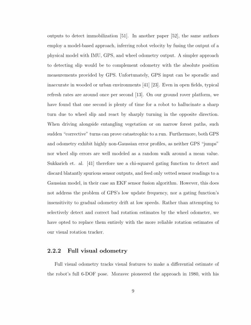
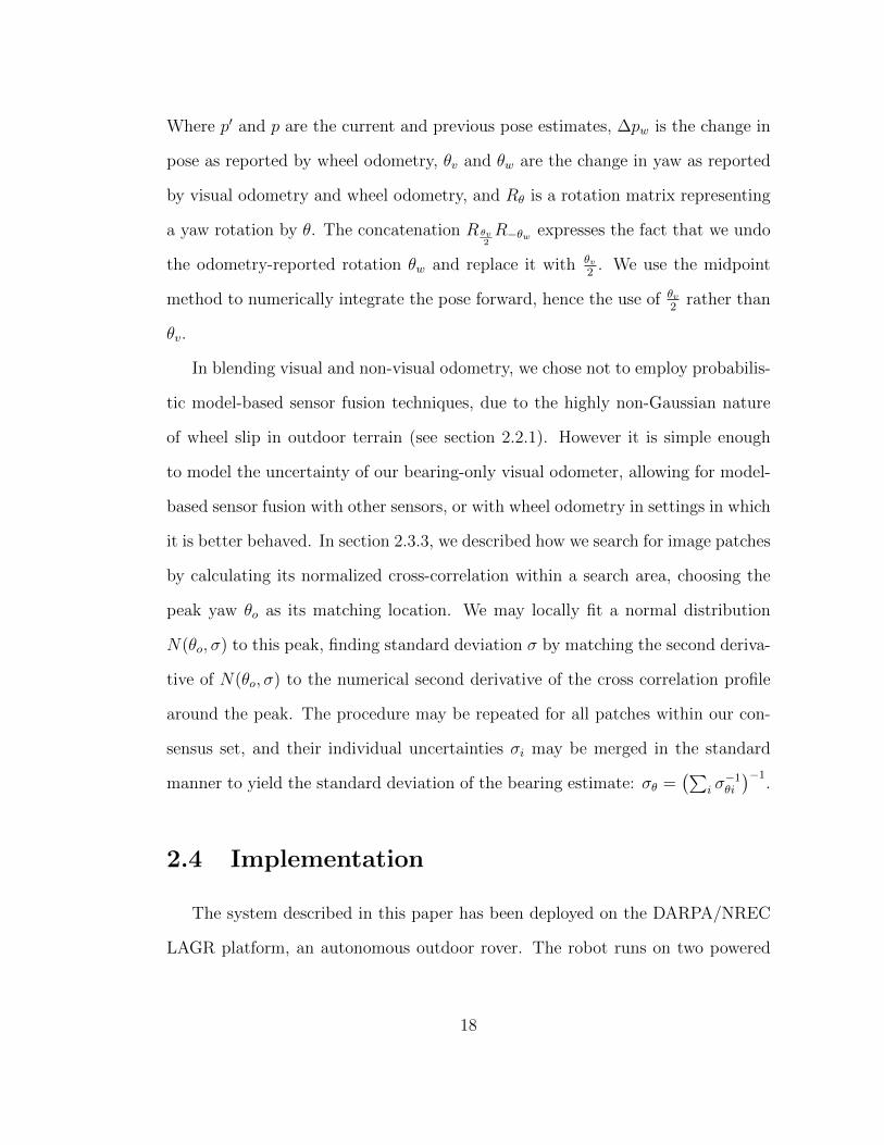
2.3 The robot’s view, while running two of the courses in figure 2.4. “Previ-

ous frame” shows the spherically projected horizon image. Harris corners

are detected in a region shown in blue, defined either as the frontal di-

rection (figure 2.3a), or as what will become the frontal direction in the

current frame, according to wheel odometry (figure 2.3b). Image patches

are sampled around the strongest corners. “Current frame” shows their

matches in the current frame. “Search windows” shows their search ar-

eas, defined to span the patch’s position in the previous frame and its

position in the current frame as predicted by wheel odometry. Figure

2.3b has wider search windows because the robot is in the middle of a

sharp turn. “Patches” shows the isolated patches. The patch framed by

yellow dots is a discarded outlier patch. Comparing the yellow rectangle

in the previous and current frames, we can see that it has shifted by one

pixel relative to the other patches. . . . . . . . . . . . . . . . . . 22

xi

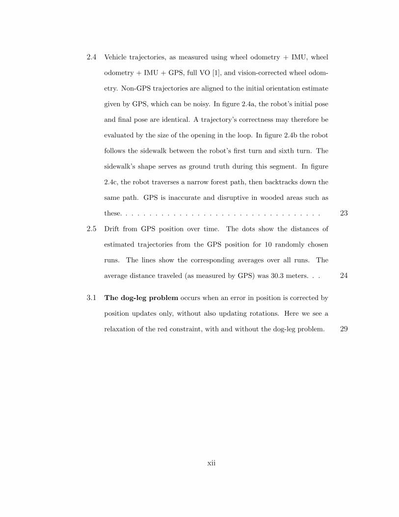
2.4 Vehicle trajectories, as measured using wheel odometry + IMU, wheel

odometry + IMU + GPS, full VO [1], and vision-corrected wheel odom-

etry. Non-GPS trajectories are aligned to the initial orientation estimate

given by GPS, which can be noisy. In figure 2.4a, the robot’s initial pose

and final pose are identical. A trajectory’s correctness may therefore be

evaluated by the size of the opening in the loop. In figure 2.4b the robot

follows the sidewalk between the robot’s first turn and sixth turn. The

sidewalk’s shape serves as ground truth during this segment. In figure

2.4c, the robot traverses a narrow forest path, then backtracks down the

same path. GPS is inaccurate and disruptive in wooded areas such as

these. . . . . . . . . . . . . . . . . . . . . . . . . . . . . . . . . . 23

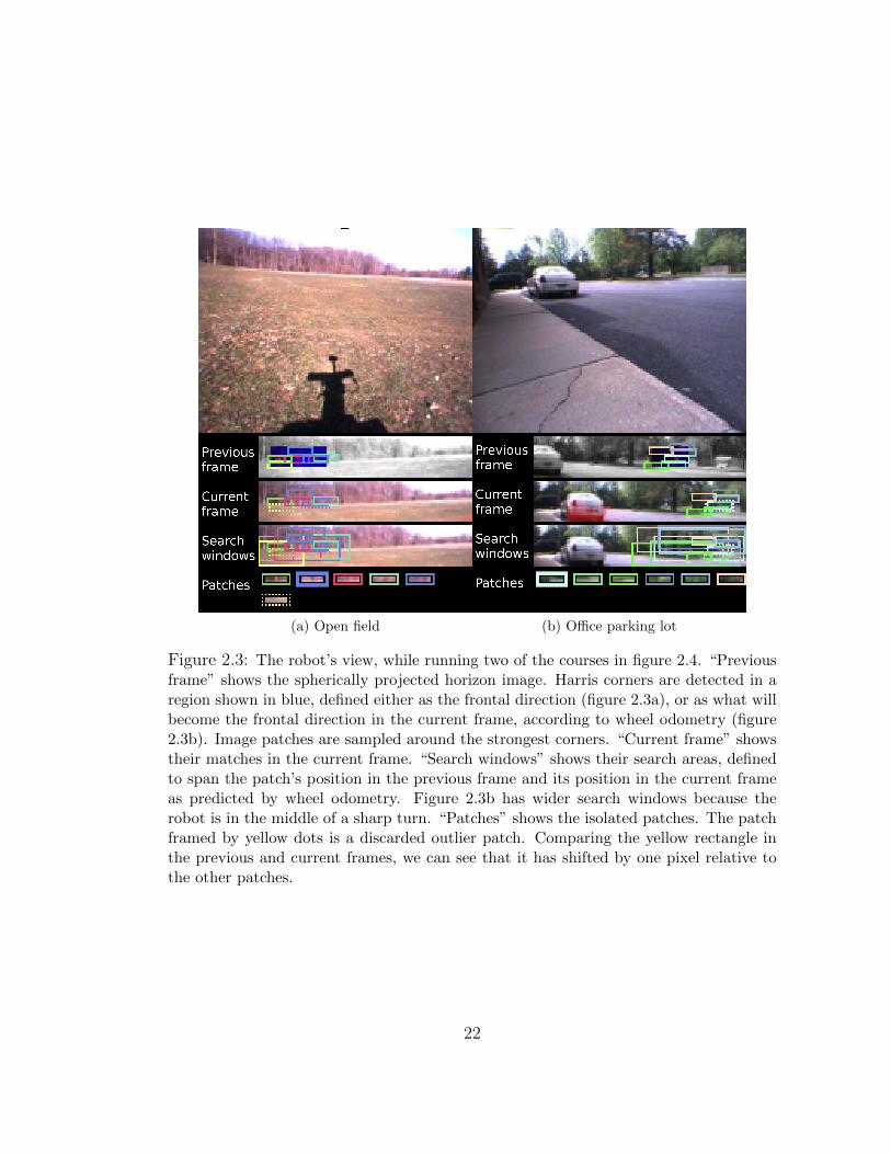
2.5 Drift from GPS position over time. The dots show the distances of

estimated trajectories from the GPS position for 10 randomly chosen

runs. The lines show the corresponding averages over all runs. The

average distance traveled (as measured by GPS) was 30.3 meters. . . 24

3.1 The dog-leg problem occurs when an error in position is corrected by

position updates only, without also updating rotations. Here we see a

relaxation of the red constraint, with and without the dog-leg problem. 29

xii

3.2 Pose tree terminology The image on the left shows a small pose graph,

with odometry edges in blue, and a loop-closing edge in red. We use a

hierarchical pose representation, defining each pose relative to its parent

in a spanning tree. Such a tree is shown in the center. The right figure

introduces some terminology: A constraint’s domain is the set of poses

whose values affect the constraint energy. The constraint’s root is the

topmost node in the path from one node of the constraint to the other.

It is not part of the constraint domain. . . . . . . . . . . . . . . . 32

3.3 χ2 error vs time, Valencia dataset The average constraint energy vs

time (in seconds) for TORO [17] and our method. For our method, we

use different values for the maximum limit Dmax on the number of poses

solved per constraint, as described in section 3.3.6. . . . . . . . . . 37

3.4 Subsampling a constraint path Subsampling a path by omitting node

p, parent of b. Node b is now acted on by a temporary constraint β

instead of α. The block corresponding to node b in the block-diagonal

hessian approximation B must be updated accordingly, using equation

3.36. Constraint β is constructed from constraints γ and α. . . . . . 43

xiii

3.5 Reordering edges and nodes: The sparsity pattern of the full square-

root information matrix (J) of the Manhattan dataset [37], constructed

from all of the edges. Each column corresponds to a node (pose), while

each row corresponds to an edge (sensor reading). In fig. 3.5a, the

rows and columns are listed in chronological order of their corresponding

sensor readings and poses. In fig. 3.5b, they are sorted as described

in section 3.3.8. This matrix has fewer sub-diagonal elements, making

it easier to upper-triangularize and solve. The left matrix took 41.52

seconds to QR-factorize with Householder reflections on a 2 GHz Intel

Core 2 Duo; the right matrix took 12.26 seconds. . . . . . . . . . . 59

3.6 Online tree balancing. From left to right: fig. 3.6a shows the sphere

dataset [17], a pose graph formed by a robot spiraling down a sphere

from top to bottom. The remaining figures show various spanning trees,

where tree depth is indicated by color (redder is deeper). Figure 3.6b

shows a pathological case of naive tree growth, in which old nodes never

change parents. Online TORO and SGD use this method. Fig. 3.6c

shows a tree built offline by simple breadth-first traversal of the graph,

as employed in [15]. This guarantees a balanced tree, but can only be

done offline, not online. Fig. 3.6d shows the tree when using dynamic

balancing, as described in section 3.3.9. . . . . . . . . . . . . . . . 60

3.7 Batch-relaxing GPS Because GPS constraints do not specify rota-

tion, relaxing them one at a time can cause spurious rotations of the

constrained node and its subtree. To lock down rotation, we relax them

together in a batch. . . . . . . . . . . . . . . . . . . . . . . . . . 61

xiv

3.8 Paris1 dataset A posegraph taken from a section of Paris, with 27093

nodes and 27716 constraints. Fig. 3.8a shows a section of the pose tree in

its initial state. Stretched constraints can be seen as red lines. Fig. 3.8b

is the same section after 10 iterations of our method, using a maximum

problem size of Dmax = 200, and no GPS constraints. The stretched con-

straints of 3.8a have collapsed; the runs that remain separated are those

without constraints tying them together. Fig. 3.8c shows a severely

under-constrained intersection, with few loop-closing constraints con-

necting adjacent runs. Such intersections can happen due to the diffi-

culty in identifying loop closures in dynamic urban environments. While

optimizing the posegraph, parallel paths with no cross-connections can

become separated. Fig. 3.8d shows the same intersection when GPS

constraints are added to one out of every 100 nodes. The GPS’ residual

vectors are visible as blue line segments. Unlike loop-closing constraints,

GPS constraints are easy to come by, limit drift in large loops, and pre-

vent separation of nearby unconnected runs. Fig. 3.8e shows a portion of

the Paris posegraph after convergence with TORO. The dog-leg problem

has caused the vehicle poses to not point along the direction of travel.

No GPS constraints were used. Fig. 3.8f shows the same portion, after

convergence with our method. . . . . . . . . . . . . . . . . . . . 62

xv

3.9 Solved maps Pose graphs, before and after 10 iterations with Dmax =

200. Pose graph sizes are given in table 3.1. Initial configurations show

the poses as set by concatenating constraint transforms down the tree, as

described in section 3.3.2. Constraint residuals are shown as brown/red

lines connecting the constraint’s desired pose to the actual pose. Brighter

red indicates higher error. Valencia (fig. 3.9c, fig. 3.9d) is shown at an

oblique angle, to better show its error residuals, which are primarily

vertical. . . . . . . . . . . . . . . . . . . . . . . . . . . . . . . . 63

3.10 Montmartre, Paris An overlay of the converged poses of fig. 3.9f on a

satellite image from Google Earth. . . . . . . . . . . . . . . . . . . 64

3.11 Online vs offline convergence Online tree-balancing incurs some ad-

ditional cost over offline operation, as shown by the rightward shift of

the green line (online) relative to the blue line (offline). Each point rep-

resents a complete loop through all edges. After the first loop, the online

algorithm revisits old edges in depth-first order. . . . . . . . . . . . 65

3.12 Graphs with large initial error Pose graphs, with noisified constraints

(sensor readings). A small random rotation around the local up axis was

multiplied onto each constraint’s rotation, causing large distortions to

accumulate over time. Pose graph sizes given in table 3.1. Constraint

residuals are shown as brown/red lines (redder = more error). . . . 66

xvi

List of Tables

2.1 CPU time per frame on a 2 GHz Pentium 4M for full VO [1] and

hybrid VO on the three courses shown in figure 2.4. . . . . . . . 21

3.1 Minimum values of Dmax needed for convergence. . . . . . . . . 45

3.2 Average and maximum time per constraint, Valencia dataset . . 56

xvii

1Introduction

Unlike other areas in computer science, mobile robotics has not generally en-

joyed an overabundance of processing power. This is sometimes the result of

designing hardware for physical robustness over speed. For example, the Mars

Exploration Vehicle’s CPU is made resistant to radiation and draws little power,

in exchange for running at a mere 20 MHz [33]. At other times, the burden of

processing high-dimensional sensor input (e.g. video) at real-time rates can leave

little processor time for anything else. Finally, and most cripplingly, human ambi-

1

tion for robotics as a field currently far outstrips its fledgling capabilities. If for no

other reason, it seems safe to assume that this last factor will keep robot processors

running at capacity for years to come.

Localization and SLAM is considered a maturing field, at least within the

static-world assumption. The current minimum bar for publication seems to be

set at real-time operation in three-dimensional, building-sized environments, and

this standard is rising rapidly. From the vantage point of this plateau, however,

we may see that many real engineering problems have been left unaddressed.

For one, the term “real-time” is often used in the weaker sense of amortized real-

time performance, wherein saturating the CPU for two full seconds can be forgiven,

so long as it is left unmolested for the next ten. This standard is insufficient for

even moderately complex systems, which will have critical components competing

with SLAM for immediate CPU time. One may lessen the blow by running the

localizer in a low-priority thread, but this introduces problems of its own. For

example, delaying large corrections to the robot location can disrupt dependent

systems such as landmark recognition and navigation. Therefore, the preferable

standard to amortized real-time performance is guaranteed real-time performance,

wherein the localizer can always process a frame’s sensor input well before the

next frame, even in the worst case. In chapter 3 we demonstrate a system that

maintains this guarantee even in city-scale environments.

Another practical concern left largely unaddressed is that optimal precision is

often not worth its cost. In chapter 2 we present a frugal visual odometry solution

that delivers 95% cost savings over conventional VO by estimating only rotation,

leaving translation to be efficiently measured by wheel odometry. While less ac-

curate than a full visual odometer, our system nonetheless delivers comparable

2

accuracy over moderate distances, while freeing up CPU time for a long-range vi-

sual traversability classifier. In off-road navigation, long-range vision is far more

valuable than pixel-perfect local accuracy. This trade-off would have been impos-

sible under a short-sighted commitment to optimal local precision.

There are exact SLAM solvers, and faster but more approximate SLAM solvers.

What these both presume is that which is more desirable will not change during

the lifetime of the robot. This is often untrue. The amount of available CPU cycles

can fluctuate sharply from frame to frame, due to the unpredictable demands of

other components as they respond to a dynamic environment. One would therefore

prefer to be able to choose the amount of time to spend on localization, where more

time translates to more precision. Chapter 3 describes a novel SLAM algorithm

with flexible cost. It will process the sensor input of a frame within a dynamically

chosen budget, which may range from O(N) to O(N2) in the size of the loop to

be closed.

Finally, many SLAM papers demonstrate “real-time operation” empirically, by

showing acceptable performance on established datasets. However, this perfor-

mance is often the result of using limited-range sensors such as laser scanners, or

operating indoors, where loop sizes are small. This experimental validation leaves

some of these SLAM solvers less than future-proof against large loops, and impend-

ing contributions from computer vision, such as long-range landmark recognition.

Both of these can play a large part outdoors. In chapter 3 we demonstrate how

to guarantee real-time performance bounds even in the face of such locally dense

graphs and large loops.

Taken together, these chapters describe localization solutions which save sig-

nificant amounts of computation over competing methods, by delivering a level

3

of precision appropriate to the task at hand. The saved cost can be used on ad-

ditional components whose value far exceeds that of an incremental increase in

precision. Furthermore, by making the cost adjustable, the H2O solver allows as

much precision as the robot can afford, thus providing an unobtrusive and reliable

bedrock upon which to build complex mobile systems.

4

2Efficient Off-Road Localization with

Visually Corrected Odometry

We describe an efficient, low-cost, low-overhead system for robot localization in

complex visual environments. Our system augments wheel odometry with visual

orientation tracking to yield localization accuracy comparable with “pure” visual

odometry at a fraction of the cost. Such a system is well-suited to consumer-

level robots, small form-factor robots, extraterrestrial rovers, and other platforms

5

with limited computational resources. Our system also benefits high-end multi-

processor robots by leaving ample processor time on all camera-computer pairs to

perform other critical visual tasks, such as obstacle detection. Experimental results

are shown for outdoor, off-road loops on the order of 200 meters. Comparisons are

made with corresponding results from a state-of-the-art pure visual odometer.

2.1 Introduction

The ability for a robot to localize itself can be critical for successful autonomous

operation. While a globally consistent solution to the localization problem must

necessarily also perform mapping [48], many applications do not require or benefit

from a globally consistent map. Locally consistent approaches such as fixed-time-

window SLAM [4] and visual odometry [1, 35] have shown great success in applica-

tions such as goal-directed navigation and localization in dynamic environments.

Wheel odometry has been a popular mainstay for robotic localization due to

its low overhead and high sampling frequency. Its accuracy however is limited by

wheel slip, a source of error that can be challenging to detect and correct without

other sensors. Wheel slip can be particularly frequent and destructive in runs over

outdoor terrain with loose or uneven ground. Full visual odometry (VO) uses fea-

ture tracking to entirely replace ground odometry, but current systems [1] require

100% of the processing time on a high-end CPU. For single-CPU autonomous

robots, this cost can be prohibitive. The cost of VO can be a burden even for

multi-CPU platforms, as it is often desirable for all camera-computer pairs to be

able to perform additional tasks, such as short-range obstacle detection, at high

framerates in their respective fields of view.

6

We have implemented a visual localization system that runs at a fraction of the

cost of state-of-the-art VO systems while maintaining comparable accuracy. On our

multi-processor, multi-camera system, this allows a single processor-camera pair

to handle VO in parallel with other visual tasks, enabling tight coupling between

localization, obstacle detection, and control. Our system can be of even more use to

robots with limited computational power, such as small robots, consumer-oriented

platforms, or extraterrestrial rovers.

We achieve this performance gain by specializing the visual odometer to the

task of tracking only one degree of freedom: the robot’s bearing. This bearing

estimate is combined with a wheel odometer’s translation estimate to yield 3-DOF

pose estimates with much-improved accuracy over wheel odometry, and compara-

ble accuracy to 6-DOF visual odometers on low-curvature terrain. The efficiency of

our system comes from the fact that tracking only the bearing allows us to operate

at much lower resolutions than would be acceptable on a 6-DOF odometer. This

is because the uncertainty of an object’s distance grows rapidly with distance at

low resolutions, while the uncertainty of its robot-relative bearing is constant. For

example, at our resolution of 160x120 pixels, an uncertainty of ±0.25 pixels trans-

lates to ±0.1 degrees of yaw, but ±1.25 meters of distance for an object 6 meters

away. Additional speedups are gained by using spherical image projection for more

reliable feature tracking, and limiting the feature tracking to windows bounded by

wheel odometer output. We show that this hybrid odometry approach achieves

much of the benefit of a full visual odometer at a greatly reduced computational

cost.

7

2.2 Related Work

There has been much work in both wheel odometry and visual odometry (VO),

while only limited attention has been paid to the intersection of the two approaches.

Schaefer et. al. [43] use wheel odometry to check the output of a full VO system

for errors arising from moving objects. Similarly, Kneip et al use inertial sensors

to provide a motion prior to increase the robustness of full VO [30]. Rather than

run full VO in parallel to wheel odometry or inertial sensors, we have focused on

how to best exploit wheel odometry to lighten the computational burden of VO.

A number of authors have used visual matching to correct IMU or GPS data on

aerial platforms [6] [3] [49]. Our system is implemented on a ground rover, where

many of the assumptions afforded in the air, such as nearly coplanar features and

slow visual flow, do not apply.

Most other work in relative pose tracking has focused either on using non-visual

sensors to detect wheel slip, or on employing full visual odometry as a complete

replacement to wheel odometry.

2.2.1 Wheel odometry correction

Wheel slip can occur in many flavors, from sudden spurts of wheel speed to

gently increasing drift. The latter in particular is difficult to detect by simple cross-

checking against motor current or inertial sensor output, requiring more nuanced

approaches. Ojeda et. al. [36] correct odometry using parametrized functions

of motor current and soil cohesion. However, Maimone et. al. [33] report that

such an approach fares poorly unless the soil consistency is nearly homogeneous.

Ward and Iagnemma train an SVM on hand-labeled odometric and inertial sensor

8

outputs to detect immobilization [51]. In another paper [52], the same authors

employ a model-based approach, inferring robot velocity by fusing the output of a

physical model with IMU, GPS, and wheel odometry output. A simpler approach

to detecting slip would be to complement odometry with the absolute position

measurements provided by GPS. Unfortunately, GPS input can be sporadic and

inaccurate in wooded or urban environments [41] [23]. Even in open fields, typical

refresh rates are around once per second [13]. On our ground rover platform, we

have found that one second is plenty of time for a robot to hallucinate a sharp

turn due to wheel slip and react by sharply turning in the opposite direction.

When driving alongside entangling vegetation or on narrow forest paths, such

sudden “corrective” turns can prove catastrophic to a run. Furthermore, both GPS

and odometry exhibit highly non-Gaussian error profiles, as neither GPS “jumps”

nor wheel slip errors are well modeled as a random walk around a mean value.

Sukkarieh et. al. [41] therefore use a chi-squared gating function to detect and

discard blatantly spurious sensor outputs, and feed only vetted sensor readings to a

Gaussian model, in their case an EKF sensor fusion algorithm. However, this does

not address the problem of GPS’s low update frequency, nor a gating function’s

insensitivity to gradual odometry drift at low speeds. Rather than attempting to

selectively detect and correct bad rotation estimates by the wheel odometer, we

have opted to replace them entirely with the more reliable rotation estimates of

our visual rotation tracker.

2.2.2 Full visual odometry

Full visual odometry tracks visual features to make a differential estimate of

the robot’s full 6-DOF pose. Moravec pioneered the approach in 1980, with his

9

work on the Stanford cart [34]. Nister et. al. [35] tracked Harris corners [19] in real

time, discarding spurious feature associations between frames using RANSAC [12].

Others have used the more recent FAST feature detector [40] in place of Harris

corners. Alternatives to RANSAC include graph-based consistency checking [24]

and exploiting the camera platform’s motion constraints [42]. Huang et. al. used

an RGBD camera to provide input to a VO system [25], whereas we used a stereo

camera, which is more appropriate for outdoor use. Agrawal et. al. boosted

accuracy by incorporating bundle adjustment to reduce drift [1]. However, their

system occupies all of the processor time on a high-end CPU, requiring additional

computers to handle other aspects of autonomous operation such as mapping and

planning. The NASA Mars Exploration Vehicle is hit particularly hard by the

computational demands of full VO, which can take up to 3 minutes per frame

on its 20 MHz processor, leading to an average movement of 10m/hour [33]. By

contrast, our system is implemented on the same robotic platform used in [1]

where one of its two camera-computer pairs is dedicated to the task of real-time

full VO. However, this leaves that camera-computer pair unable to perform other

potentially critical tasks on its field of view, such as obstacle detection. For this

reason, we have chosen our more lightweight approach. Kaess et al exploit the

same core observation that we do, namely that faraway features are useful for

estimating rotation, while nearby features are better for estimating translation

[28]. They exploit this observation to increase robustness to degenerate input,

while we use it to increase speed.

10

2.3 Algorithm

In the interest of keeping running costs down, our system tracks only six patches

per frame, tracking wide image patches at low resolution. The system samples

patches from a region around the horizon, interpreting their horizontal motion

from frame to frame as a rotation of the robot. There are two challenges to this

approach: one is that a small number of features may be less robust to mismatches.

The other is that a robot driving in a straight line will see features drift towards the

sides of the image as it drives by (“parallax drift”). Under a naıve implementation,

such horizontal motion in the image would be incorrectly interpreted as a rotation.

In this section we give a walkthrough of our algorithm, paying particular attention

to the solutions to the above problems. The overall algorithm is as follows:

1. Re-map the image to remove feature size distortions due to planar projection.

2. Sample features from a small region of the previous frame selected using

wheel odometry.

3. Search for the sampled features in the current frame, again limiting the search

area using wheel odometry.

4. Cross-validate the features’ motions between frames and discard any outliers.

5. Localize the robot in the current frame by replacing the wheel odometry’s ro-

tation estimate with that of the visual odometer, and rotating the translation

estimate by the difference in rotations.

While the sampling and searching steps above use wheel odometry, they do so in a

manner that is not adversely affected by wheel slip, as will be discussed in section

2.3.3.

11

(a) Camera image (b) Spherical image

Figure 2.1: A rectified camera image and its spherical transform. The asymmetry ofthe spherical image is due to the fact that the camera is pointed off to the left anddown, with some axial roll. The robot is pointed straight at the area highlighted byfour yellow dots, placed at pitch and yaw values [0.03, 0.1], [0.03,−0.1], [−0.03,−0.1],and [−0.03, 0.1], in radians. After the transformation, these points form an axis-alignedrectangle around the frontal direction. In practice, we transform only the portion of thecamera image roughly located around the horizon, highlighted by the green rectangleabove.

2.3.1 Re-map image to a spherical projection

Because we track a small number of image patches per frame, care must be

taken to minimize the number of mismatched patches. We use wide patches sub-

tending eight degrees of yaw, as larger patches tend to be more distinctive. How-

ever, such large features stretch when moved from the center of the image to the

edges, where each pixel subtends a smaller solid angle. This distortion can cause

mismatches when searching for features that have moved from the center of the

image to near an edge, or vice-versa. To remove this distortion, we remap the cam-

era image using a “spherical projection”, where each pixel row and column covers

a fixed amount of vehicle-relative pitch and yaw [φp, θp], respectively (figure 2.1).

We define the mapping from camera image coordinates [i, j] to spherical image

12

'

d

r

r si

n

r cos ­ d

Figure 2.2: Parallax from pure forward motion. We wish to limit our attentionto objects which will not shift under parallax from frame to frame. In a spherical imagewhere each pixel subtends θp radians of yaw, this requires that the bearing θ of the objectnot change more than θp/2. Given upper limits on θ and the frame-to-frame translationd, we may solve for a minimum distance r. We avoid parallax by detecting distance usingstereo data calculated earlier for obstacle detection, and ignoring all features closer thanr.

coordinates [k, l] as:

k(i, j) = (φ(i, j)− φo)/a (2.1)

l(i, j) = (θ(i, j)− θo)/a (2.2)

Here, a is a chosen ratio of radians per pixel, and [φo, θo] is the pitch and yaw

of the view ray corresponding to the upper-left pixel in the spherical image. We

choose a as being the radians-per-pixel of the center pixel in the planar image. We

perform this mapping using a precalculated coordinate look-up table.

2.3.2 Sampling features

Even when the robot is moving straight forward, any feature except for those

directly in front of the robot will experience nonzero drift towards the side of

the image as the robot drives by. If we are to interpret the horizontal motion

of features as robot rotation, we must limit our features to those for which this

13

frame-to-frame “parallax drift” is less than half a pixel in the spherical image, and

therefore undetectable. As shown in figure 2.2, this constraint defines a minimum

value for a feature’s distance r as a function of its bearing θ, the maximum possible

travel of the camera between frames d, and the yaw subtended by a pixel in the

spherical image θp:

rmin =d tan(θp/2 + θ)

cos θ tan(θp/2 + θ)− sin θ(2.3)

With a sufficiently reliable stereo vision system with which to estimate r, one

could threshold all features in the image by their distance. However, the threshold

rmin increases with bearing θ, and stereo depth is unreliable for faraway features at

low image resolutions. We therefore opt to limit our sampling to a small range of

yaw −θmax < θ < θmax centered on the frontal direction θ = 0. We then substitute

θmax for θ in equation 2.3 to derive a corresponding minimum distance rmin. Any

feature closer than rmin is deemed unfit for use. When an insufficient number of

viable landmarks are found in a particular frame, the pose for that frame is esti-

mated using wheel odometry. In practice, this happens relatively rarely outdoors.

Even in dense forests such as the one in figure 2.4c, the many nearby obstacles

(trees) caused our hybrid VO system to defer to wheel odometry on only 7.9% of

the frames. We found that this was sufficiently low to maintain good performance

on uneven and slippery forest ground. Two exceptions where distal features may be

intermittent are areas that are dense with eye-level vegetation, or extremely hilly

areas where the terrain regularly rises to eye level within rmin meters. The former

situation can be mitigated by slowing down to reduce d, and therefore reduce rmin,

when VO finds itself frequently delegating to wheel odometry. The latter case of

14

severely hilly terrain presents mapping difficulties for any 3-DOF model, though

our visual tracker still presents an improvement over wheel odometry for control

purposes.

On our system, we estimate distance using the dense stereo image already

calculated by another component for the purposes of obstacle detection. If no

such calculation is already being done, the approach of [1] may be used, where

stereo disparity is calculated for each patch rather than for all pixels. Our use

of stereo information is distinguished by its low requirement for depth precision.

We need only establish whether a patch is close enough to drift due to parallax

between neighboring frames. The lower the resolution, the looser this requirement

becomes, as features need to drift farther to cause noticeable pixel shift. This low

dependence on depth precision enables our method to operate efficiently on low

resolution video. By contrast, pure VO methods that use the depth estimate to

measure translation are more sensitive to the high depth uncertainty at low image

resolutions.

The choice of θmax can be made based on the robot’s expected speed, environ-

ment, and camera geometry. On our platform, the cameras point off to the sides,

thereby making the frontal direction close to one side of the spherical image (see

figure 2.1b). We therefore chose θmax to be the absolute value of the yaw of that

side, namely ±0.09 or ±0.14 radians depending on the eye. This left 15% to 23%

of the horizon image available for sampling. Using these θmax values, along with a

d of 0.13 meters (1.3 m/s / 10 Hz), equation 2.3 yields minimum distances rmin of

2.42m and 3.69m.

The region defined by −θmax < θ < θmax is further shrunk on all sides by half

the patch dimensions before searching for Harris corners in one of its channels.

15

These corners are used to find suitable points from which to sample RGB patches.

The shrinkage is done to ensure that patches centered on these corners are com-

pletely contained within −θmax < θ < θmax. The horizon images labeled “previous

frame” in figure 2.3 show this region in blue. As each image patch is selected, the

Harris corners under that patch are set to zero as a form of non-max suppression.

We sample 6 patches measuring 13 x 3 pixels, or 7.6 by 1.75 degrees of solid angle,

or 11% by 3% of the field of view. Note that while we sample in a narrow region,

the search region is not so constrained. Therefore, θmax does not present a limit

on our robot’s rotation rate.

2.3.3 Searching for patches

In outdoor environments, it is a common occurrence for the robot to rotate less

than reported by wheel odometry (“wheel slip”). The opposite case of the robot

rotating significantly more than the wheels (“wheel skid”) is far less common under

vehicle speeds typically operated under by autonomous vehicles [52]. We therefore

trust our odometry to set an upper limit on the expected patch motion from frame

to frame. Vehicles that do operate at skid-inducing speeds may choose to employ

low-resolution whole-image matching, used by Klein et al [29] for efficient high-

speed tracking, to provide another prior for the patch locations. When searching

for image patches, we limit our search window to a region that encompasses the

patch’s position in the previous frame and the patch’s position in the current frame,

as predicted by wheel odometry. This window is inflated on all sides by half the

patch dimensions for an added measure of safety. We apply a normalized cross-

correlation of the image patch with this search window, and choose the maximum

as the best-matching location.

16

On our platform, the camera used for VO points off to one side, putting the

frontal direction near the side of the image. Features sampled from this area are

easily scrolled off that frontal side of the screen when the robot turns away from it.

We therefore choose the sampling location using wheel odometry. If it indicates a

turn away from the frontal side, we sample not from the previous image’s frontal

region, but from the area that will become the frontal region in the current frame,

according to odometry. In order for both these regions to be scrolled off the screen,

almost the entire image must be scrolled off-screen in either direction. This is an

impossibility on our system, given its maximum turn rate of π radians per second.

2.3.4 Cross-validate matches

The change in yaw of an image patch from the previous frame to the current

frame is that patch’s estimate of the robot’s rotation. To detect outliers, we cross-

validate by having each patch “vote” for every other patch whose estimate differs

by less than θp. Patches whose vote tally is more than half the number of patches

are deemed reliable, while others are rejected as outliers. The rotation estimate

shared by all inliers is taken as the robot’s rotation between the previous and

current frames. When using a small number of patches, a pair of frames may

occasionally present no patches with a sufficient number of votes. On such frames

we let the wheel odometer supply the change in pose.

2.3.5 Localizing the robot

The robot’s current pose is estimated as:

p′ = p+R θv2R−θw∆pw (2.4)

17

Where p′ and p are the current and previous pose estimates, ∆pw is the change in

pose as reported by wheel odometry, θv and θw are the change in yaw as reported

by visual odometry and wheel odometry, and Rθ is a rotation matrix representing

a yaw rotation by θ. The concatenation R θv2R−θw expresses the fact that we undo

the odometry-reported rotation θw and replace it with θv2

. We use the midpoint

method to numerically integrate the pose forward, hence the use of θv2

rather than

θv.

In blending visual and non-visual odometry, we chose not to employ probabilis-

tic model-based sensor fusion techniques, due to the highly non-Gaussian nature

of wheel slip in outdoor terrain (see section 2.2.1). However it is simple enough

to model the uncertainty of our bearing-only visual odometer, allowing for model-

based sensor fusion with other sensors, or with wheel odometry in settings in which

it is better behaved. In section 2.3.3, we described how we search for image patches

by calculating its normalized cross-correlation within a search area, choosing the

peak yaw θo as its matching location. We may locally fit a normal distribution

N(θo, σ) to this peak, finding standard deviation σ by matching the second deriva-

tive of N(θo, σ) to the numerical second derivative of the cross correlation profile

around the peak. The procedure may be repeated for all patches within our con-

sensus set, and their individual uncertainties σi may be merged in the standard

manner to yield the standard deviation of the bearing estimate: σθ =(∑

i σ−1θi

)−1.

2.4 Implementation

The system described in this paper has been deployed on the DARPA/NREC

LAGR platform, an autonomous outdoor rover. The robot runs on two powered

18

wheels and two passive casters, and takes input from wheel encoders, an IMU,

and a GPS unit. In addition it takes visual input from two stereo camera pairs,

pointing slightly to the left and to the right, with fields of view that overlap slightly

around the frontal direction. The robot provides three user-accessible computers,

one of which runs the VO system described in this paper. We have implemented all

software components in Lush, an interpreted language with compilable functions.

The visual odometer is entirely compiled, and runs on one of the camera computers.

We captured the camera images at a low resolution of 160 x 120 pixels, and used six

image patches of 13 x 3 pixels. The Intel Performance Primitives (IPP) library was

used for the spherical image transform, Harris corner detection, and normalized

cross-correlation. The hybrid VO system runs within the same thread as the short-

range stereo-based obstacle detector [44], running at 6 Hz. The processor time is

also shared by a long-range (5 to 150 meters) obstacle detector [18] running in

a separate thread at 1 Hz. The “IMU + wheel” and “GPS + IMU + wheel”

trajectories shown in figure 2.4 were calculated using tuned EKF pose estimators

provided with the platform.

2.5 Results

The hybrid VO system has been tested on various types of outdoor terrain

including the area around an office building, an open field, and a narrow path

through a forest. For the results presented here, we recorded logs in these settings,

and ran both our hybrid VO and the full 6-DOF VO of [1] on them, as a benchmark

for accuracy and processor time. Figure 2.4 shows the pose trajectories of three

runs. Predictably, wheel odometry fused with IMU consistently fares the worst.

19

The EKF fusion of wheel odometry, IMU, and GPS does better, except in the forest

where the GPS signal can be both sporadic and inaccurate. Even with clear GPS

reception, the GPS-aided trajectory suffers from discontinuities due to satellites

coming in and out of reception. Full VO and hybrid VO perform comparably in

all three runs, except for figure 2.4b, where a forward wheel slip was deliberately

induced by running the robot up against a curb that was too high to surmount.

All but the full visual odometer are fooled into believing that the robot made it

over the curb. The plot in 2.4c shows the robot going down a narrow path through

a forest. Accurate, high-frequency estimates of the robot bearing are particularly

important in such settings, where false rotations due to wheel slip are frequent,

and can cause a robot to counter-steer into entangling obstacles on each side. The

hybrid VO retraces the path accurately after a quick 180-degree turn.

Figure 2.5 shows the drift from GPS (taken here to represent ground truth) over

time for wheel odometry, hybrid VO, and pure VO. The data is from 10 randomly

chosen runs, manually vetted for inaccurate GPS such as that of figure 2.4c.

The average CPU cost per frame of each of these runs is reported in table 2.1.

The runtimes shown are those of a Pentium 4M laptop at 2 GHz, running off of

image and sensor data logged by the robot. The robot’s CPUs are approximately

2.5 times faster. While our system does not track translations, it does use range

information to rule out features that are too close to the robot. As discussed in

section 2.3.2, we get this information “for free” by appropriating the stereo image

already calculated by our obstacle classification system. If no such stereo image

data is available, we can also adopt the approach of [1], where a patch is searched

for in the other stereo camera to estimate distance on a per-patch rather than

per-pixel basis. In table 2.1, the runtimes for running just the hybrid VO, and for

20

Table 2.1: CPU time per frame on a 2 GHz Pentium 4M for full VO [1] and hybridVO on the three courses shown in figure 2.4.

Log file Full VO Hybrid VO + range Hybrid VOField Loop 266 ms 11.5 ms 8.0 ms

Building Lap 238 ms 11.0 ms 8.2 msForest Path 153 ms 14.0 ms 9.3 ms

running the hybrid VO with per-patch stereo matching, are shown separately. The

full VO runtime is best compared to the latter.

2.6 Conclusions and Future Work

We have presented an efficient hybrid wheel/visual odometer capable of local-

izing an autonomous robot in unstructured outdoor terrain at 5 to 10 percent of

the computational cost of existing VO systems. Hybrid VO has the potential to

enable accurate visual localization on platforms for which previous VO systems are

prohibitively demanding. We have tested our system in outdoor terrain of varying

visual complexity, including open fields with minimal visual features, and forest

paths where GPS is error-prone and roots and leaves make wheel slip frequent.

We have demonstrated that faraway features can be used to estimate side-to-

side rotation independently of the other degrees of freedom. As mentioned earlier,

Kaess et. al. use a similar method, and follow up by estimating translation using

nearby features. This is done to boost robustness to degenerate data [28]. We

believe, however, that a similar approach can be taken with a different focus: to

improve speed for 6-DOF VO, as we have done for 3-DOF VO.

21

(a) Open field (b) Office parking lot

Figure 2.3: The robot’s view, while running two of the courses in figure 2.4. “Previousframe” shows the spherically projected horizon image. Harris corners are detected in aregion shown in blue, defined either as the frontal direction (figure 2.3a), or as what willbecome the frontal direction in the current frame, according to wheel odometry (figure2.3b). Image patches are sampled around the strongest corners. “Current frame” showstheir matches in the current frame. “Search windows” shows their search areas, definedto span the patch’s position in the previous frame and its position in the current frameas predicted by wheel odometry. Figure 2.3b has wider search windows because therobot is in the middle of a sharp turn. “Patches” shows the isolated patches. The patchframed by yellow dots is a discarded outlier patch. Comparing the yellow rectangle inthe previous and current frames, we can see that it has shifted by one pixel relative tothe other patches.

22

(a) Field Loop: A closed loop around two tree clusters.

(b) Building Lap: A partial loop around a building.

(c) Forest Path: Down a narrow forest path and back.

Figure 2.4: Vehicle trajectories, as measured using wheel odometry + IMU, wheelodometry + IMU + GPS, full VO [1], and vision-corrected wheel odometry. Non-GPStrajectories are aligned to the initial orientation estimate given by GPS, which can benoisy. In figure 2.4a, the robot’s initial pose and final pose are identical. A trajectory’scorrectness may therefore be evaluated by the size of the opening in the loop. In figure2.4b the robot follows the sidewalk between the robot’s first turn and sixth turn. Thesidewalk’s shape serves as ground truth during this segment. In figure 2.4c, the robottraverses a narrow forest path, then backtracks down the same path. GPS is inaccurateand disruptive in wooded areas such as these.

23

Figure 2.5: Drift from GPS position over time. The dots show the distances of estimatedtrajectories from the GPS position for 10 randomly chosen runs. The lines show thecorresponding averages over all runs. The average distance traveled (as measured byGPS) was 30.3 meters.

24

3Hybrid Hessians for SLAM with Tunable

Cost and Accuracy

We present Hybrid Hessian Optimization (“H2O”), an online 3D SLAM algo-

rithm with flexible per-frame cost. Our main contribution is to allow the robot

to choose how much computation to spend on SLAM in a given timestep. Set

to maximum accuracy, our method gives the same result as exact solvers. Set

to maximum speed, our method achieves linear-time speed, like fast stochastic

25

solvers, while still maintaining better accuracy. How much computation should be

spent on SLAM in a given frame? This decision belongs on the field, not in the

design room. H2O enables this flexibility.

In addition, H2O combines strengths found individually in exact and stochastic

solvers, but not together. Like exact methods, it can process GPS constraints

without the pose staggering seen in stochastic solvers (the ”dog-leg problem”).

Like stochastic methods, it is robust against noisy input, which can trap exact

methods in local minima.

We present results from the Google Street View database, and compare our

method with results from TORO, one of the fastest stochastic solvers. We show

that our solver is able to achieve higher accuracy while operating within real-time

bounds. The open-source code is available online at http://mkg.cc.

3.1 Introduction

Simultaneous localization and mapping, or SLAM, is a critical prerequisite to

autonomous mobile operation. Put differently, SLAM typically serves as a foun-

dation for higher-level tasks, rather than itself being the raison d’etre of a robot.

It is therefore important that the SLAM cost be controllable, to accommodate

unpredictable CPU demands made by other components in the field.

A common solution is to run SLAM in a separate thread, which can be de-

prioritized as necessary. There are a number of drawbacks with this approach. For

one, this may delay the closing of newly discovered loops, exactly at the moment

when this loop-closure is most needed. For example, making the correct turn at

an intersection may depend on solving the loop-closure introduced by that very

26

intersection. Furthermore, running SLAM in a separate thread prevents it from

directly providing the current pose estimate. This necessitates a separate local

odometry system for this task, increasing system complexity. Finally, delaying a

loop closure caused by one landmark can cause subsequent landmark associations

to suffer, due to uncorrected drift.

We present a method that allows the user to specify the amount of CPU time to

use in a given SLAM update, where more time yields more accuracy. This allows

our SLAM algorithm to stay within the control loop, providing the most recent

pose estimate directly to the rest of the system without need of thread synchro-

nization or odometry subsystems. It processes simple odometry-based updates in

the expected O(1) time, while loop closures cost O(N) to O(N2) time in the size

of the loop.

This controllable cost is the salient feature of H2O. However, H2O also combines

several strengths seen individually in other SLAM algorithms, but not together.

From stochastic methods, it inherits a robustness to sensor noise and poor initial

poses, along with quick, real-time closure of large loops in (if so chosen) O(N)

time. From exact methods, it inherits smooth loop closures without “dog-leg” dis-

continuities, and the ability to process position-only or orientation-only constraints

such as GPS or compass input.

We demonstrate the above features on both commonly used datasets and real-

world urban data taken from the Google Street View database. The source code

is available online at http://mkg.cc.

27

3.2 Related Work

Early filter-based SLAM algorithms, such as EKF SLAM, incorporated new

observations into an Extended Kalman Filter (EKF) [46], at a cost of O(N3) in

the size of the map. Updates start to fall below real-time performance with as few

as 200 landmarks, which for visual SLAM can amount to a handful of rooms [9].

Performance can be improved by selective sparsification of the information matrix,

[47, 50], but reconstructing the map from this matrix remains costly.

A more recent improvement is the “pose graph” formulation of SLAM, which

represents robot and landmark poses as nodes, constrained to each other by spring-

like edges, representing observations. Relaxing this node-spring graph yields the

least-squares optimal estimate of all poses given all observations. Doing so naively

with dense Gauss-Newton minimization costs O(N3) in the number of nodes, but

by exploiting the sparsity of the graph, typical SLAM methods do far better. The

many methods using this representation can be roughly divided into “exact” and

“stochastic” methods.

In machine learning, stochastic optimization is often preferred over exact op-

timization for its fast convergence and robustness to local minima [5, 32]. From

stochastic optimization, SLAM methods such as SGD and TORO [17, 37] borrow

the idea of relaxing one constraint at a time. This results in fast-converging up-

dates whose very inexactness helps to escape from local minima that would trap

an exact solver [38]. Such local minima are a risk when the initial pose estimate is

far from the global minimum due to noisy sensors such as GPS. H2O is similarly

capable of recovering solutions from poor initial estimates by noisy sensors.

Unfortunately, both SGD and TORO get their speed by neglecting off-diagonal

terms in the information matrix. This de-correlates position and rotation variables,

28

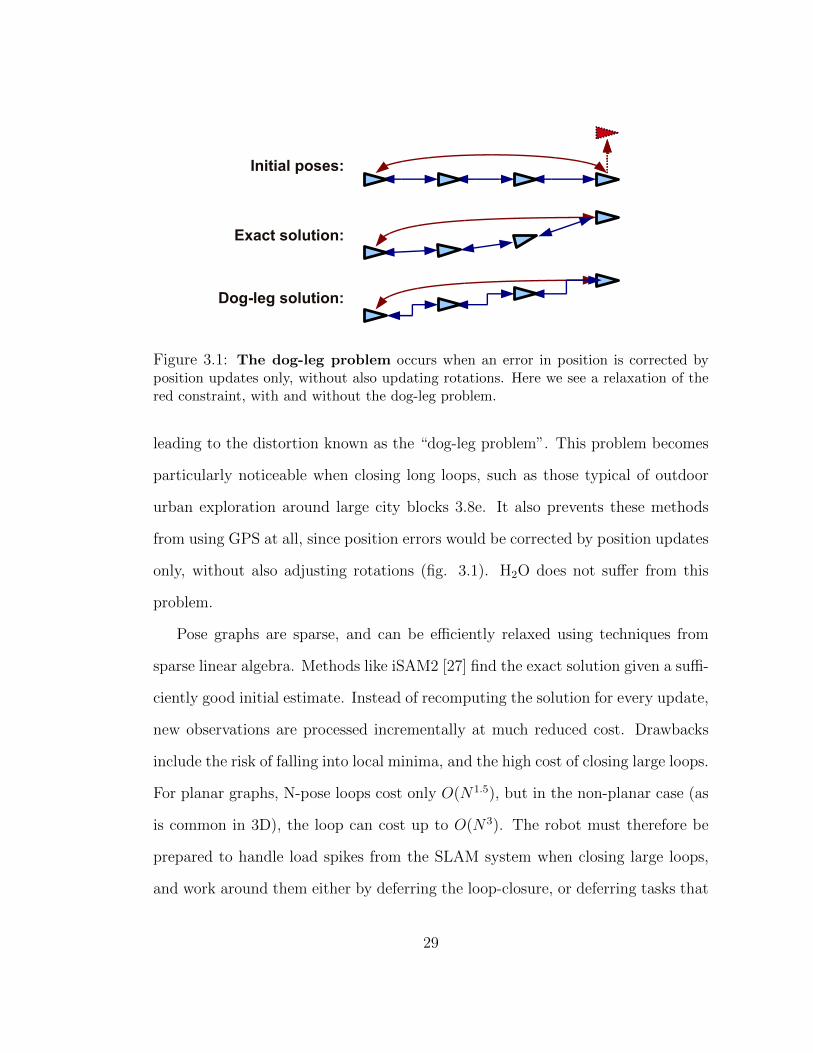
Figure 3.1: The dog-leg problem occurs when an error in position is corrected byposition updates only, without also updating rotations. Here we see a relaxation of thered constraint, with and without the dog-leg problem.

leading to the distortion known as the “dog-leg problem”. This problem becomes

particularly noticeable when closing long loops, such as those typical of outdoor

urban exploration around large city blocks 3.8e. It also prevents these methods

from using GPS at all, since position errors would be corrected by position updates

only, without also adjusting rotations (fig. 3.1). H2O does not suffer from this

problem.

Pose graphs are sparse, and can be efficiently relaxed using techniques from

sparse linear algebra. Methods like iSAM2 [27] find the exact solution given a suffi-

ciently good initial estimate. Instead of recomputing the solution for every update,

new observations are processed incrementally at much reduced cost. Drawbacks

include the risk of falling into local minima, and the high cost of closing large loops.

For planar graphs, N-pose loops cost only O(N1.5), but in the non-planar case (as

is common in 3D), the loop can cost up to O(N3). The robot must therefore be

prepared to handle load spikes from the SLAM system when closing large loops,

and work around them either by deferring the loop-closure, or deferring tasks that

29

depend on it.

Some authors have worked around this cost by limiting the scope of SLAM

to a local region around the robot. Bibby et al do this to gain a measure of

robustness to moving features [4]. Sibley performs local relaxation with similar

goals to ours: to maintain real-time performance [45]. While this does boost

speed, it is not without drawbacks. Faraway landmarks, if they are retained at

all, can drift, making it difficult to detect them for loop-closure once the robot

returns to them. Also, keeping the map in a single consistent coordinate frame

can help with collaborative mapping, or alignment with prior surveying, such as

aerial imagery or GIS. Finally, if a loop size exceeds the local relaxation bounds,

these methods must choose between closing the loop (at full cost) or leaving a

discontinuity in the loop. For these reasons, we have chosen to focus on real-time,

globally consistent SLAM.

The HOG-MAN algorithm [16] also performs local SLAM, but maintains global

consistency by connecting a simplified, easy-to-solve pose graph to the real pose

graph. The simple graph can be solved quickly, maintaining global consistency,

while local SLAM is performed on local regions of the full-resolution graph. The

cost of closing a loop remains unmitigated, however, costing up to O(N3) in the

size of the loop.

In [10], Dellaert et al propose a two-pass solution, in which a sparse linear solver

first relaxes only the “local” edges. The result is used to precondition a conjugate-

gradient step to relax the non-local “loop” edges. H2O also uses a preconditioner

to regularize the relaxation of expensive edges. However, these edges are typically

relaxed one at a time, enabling online operation.

30

3.3 Algorithm

In this section, we first review background on the pose graph SLAM repre-

sentation, our hierarchical parametrization, and linearized SLAM updates. We

then introduce H2O in terms of this background, starting with the most common

case of relaxing one edge at a time. We then generalize to relaxing any arbitrary

set of edges and nodes, while maintaining global consistency for the rest of the

map. Finally, we demonstrate dynamic reparametrization, and its importance to

guaranteeing real-time performance on all frames.

3.3.1 Pose Graphs

This work concerns itself with the pose graph formulation of SLAM. A pose

graph is formed of nodes, representing poses, and edges, which connect two poses,

and represent a sensor reading of their relative pose. For example, an odometer

may measure the relative transform from the previous pose a to the current pose b

to be transform k. We connect poses a and b by an edge representing this reading.

This edge defines an energy function that penalizes deviations of the relative pose

p = a−1b from its measured value k:

E = (k − p)TS(k − p) (3.1)

Here S is the inverse covariance of the odometry sensor, so labeled because it

represents the “stiffness” of the spring-like edge connecting a and b.

Note that poses may represent current and prior robot poses, and poses of

any landmarks being tracked. Edges are sensor-agnostic. Their relative pose es-

timates may come from laser scan-matching, IMU, visual odometry, etc. Global

31

Representation tree:Constraint graph:

loop-closing constraint

odometry constraint

Constraint root

Constraint

Constraint domain

Constraint terminology:

Figure 3.2: Pose tree terminology The image on the left shows a small pose graph,with odometry edges in blue, and a loop-closing edge in red. We use a hierarchical poserepresentation, defining each pose relative to its parent in a spanning tree. Such a treeis shown in the center. The right figure introduces some terminology: A constraint’sdomain is the set of poses whose values affect the constraint energy. The constraint’sroot is the topmost node in the path from one node of the constraint to the other. It isnot part of the constraint domain.

sensors such as GPS and compasses are no exception: they constrain the relative

position/rotation between the earth node (a landmark of sorts) and a robot pose.

SLAM thus reduces to a nonlinear minimization problem: we wish to find the

values of a, b, and all other poses, which give the global minimum of the sum of

edge energies. When edge energies are interpreted as log-probabilities, this yields

the maximum a posteriori estimate of all poses given all sensor inputs.

32

3.3.2 Pose Trees

Like [17], we use a spanning tree of the pose graph to define a hierarchical

parametrization, where we define each pose in coordinates relative to its parent in

the tree. Fig. 3.2 shows a pose graph, and one possible pose tree that spans it. We

now introduce some terminology. The “path” of the edge is the set of nodes on the

path through the tree from a to b. The “root” of the edge is the node in this path

with the smallest tree depth. This node does not affect a and b’s relative pose p,

since translating or rotating the root merely translates or rotates its entire subtree

together. All other nodes on the path do affect p and the edge energy (3.1), and

for this reason, we call them the edge’s “domain”. When SLAM relaxes an edge

to a lower energy, only its domain nodes are moved.

We can accommodate GPS, compass, and other global-coordinate sensors by

placing at the root of the tree a node representing the earth. For example, a GPS

reading on node a is an edge between the earth node and a, constraining their

relative position. Because the earth is at the root of the tree, it is outside of any

edge’s domain, and is therefore left unchanged by SLAM, as is appropriate.

3.3.3 Linearized updates

We represent our poses as 7-dimensional vectors composed of a position vector

and quaternion (quaternions are re-normalized after each update). We collect all

poses in a single vector z. For a constraint c connecting poses a and b, Let fc(z)

be the relative pose between a and b. Rewriting p in (3.1) as fc(z), we get this

33

expression for edge energy Ec:

Ec(z) = (fc(z)− kc)TSc(fc(z)− kc) (3.2)

In EKF terminology, fc is the prediction function, kc is the “observation”, and Sc

is the inverse of the sensor covariance matrix.

We may use Cholesky factorization to split Sc into Sc = LcLTc . We then define

the edge residual rc as:

rc(z) = LTc (fc(z)− kc) (3.3)

Plugging (3.3) into (3.2) we get a simpler form:

Ec = rTc rc (3.4)

The edge Jacobian Jc is the derivative of rc(z), evaluated at the current value

z = z:

Jc = ∂rc∂z

∣∣∣z

(3.5)

=

[∂rc∂z1

∂rc∂z2

· · · ∂rc∂zN

]∣∣∣∣z

(3.6)

The Jacobian above is a row of 7×7 blocks of the form ∂rc∂zi

, where zi is the i’th pose.

Because rc only depends on those poses in edge c’s domain, blocks corresponding

to other poses are all zero, making J sparse.

Stacking the Jacobians and the residuals of all M edges, we get the total Ja-

cobian J and total residual r:

34

J =

J1

...

JM

(3.7) r =

r1

...

rM

(3.8)

The total energy E is the sum of edge energies Ec:

E =∑c

Ec (3.9)

=∑c

rTc rc from (3.4) (3.10)

= ‖r‖2 from (3.8) (3.11)

To minimize E, we start by linearizing it around z:

E ≈ ‖r(z) + Jx‖2 (3.12)

We seek a perturbation x to poses z that will minimize E.

Differentiating (3.12) with respect to x and setting it to zero, we arrive at the

normal equations of the Gauss-Newton method:

2JT (Jx+ r) = 0 (3.13)

Hx = −JT r, (3.14)

Here H is JTJ , also known as the approximated Hessian or the information ma-

trix. Equation 3.14 may be upper-triangularized by the Cholesky decomposition

35

H = RTR, followed by one back-substitution:

RTRx = −JT r (3.15)

Rx = b (back-substituted RT ) (3.16)

Back-substituting R then solves for x.

We can also arrive at 3.16 by another route, by setting Jx + r = ~0 and QR-

factorizing J :

Jx = −r (3.17)

QRx = −r (3.18)

Rx = −QT r (3.19)

Rx = b (3.20)

This is the approach taken by Dellaert and Kaess in√SAM [11]. We note that

when J is nearly upper-triangular, this QR-factorization can take O(N2) time, as

opposed to the O(N3) taken to Cholesky-factorize the normal equations. We will

exploit this fact in section 3.3.5 to efficiently solve for stochastic updates.

Having solved for update x, we add it to pose parameters z:

z ← z + x (3.21)

This is followed by normalizing the quaternions in z.

36

0 10 20 30 40 50 60

Tim e (seconds)

10-3

10-2

10-1

100

101

Lo

g(a

ve

rag

e e

ne

rgy

pe

r co

nstr

ain

t)

TORO

D_m ax = 75

D_m ax = 100

D_m ax = 150

D_m ax = 200

Figure 3.3: χ2 error vs time, Valencia dataset The average constraint energy vstime (in seconds) for TORO [17] and our method. For our method, we use differentvalues for the maximum limit Dmax on the number of poses solved per constraint, asdescribed in section 3.3.6.

3.3.4 Stochastic Updates

The update x described above is expensive to evaluate, since it is calculated

using all edges in the graph. An alternative is to inexpensively calculate one ap-

proximate update xc from each edge c. Such “stochastic” updates have a long

history in machine learning [5, 32], as they converge much more quickly than exact

updates, and provide some robustness to local minima [22, 39]. The robustness

arises from the fact that stochastic optimizers experience some “jitter” in their

trajectory towards the local minimum, which can help escape shallow local min-

37

ima. Oscillations due to the inexactness of these updates are mitigated by using

a decaying learning rate, as will be discussed in section 3.3.11. In this section we

derive our expression for xc.

Plugging (3.7) and (3.8) into the right-hand-side of (3.14) gets:

Hx = −∑c

JTc rc (3.22)

This lets us express the total update x as a sum x =∑

c xc of constraint-specific

updates xc, where:

xc = −H−1JTc rc (3.23)

In practice, we compute xc by solving the linear system:

Hxc = −JTc rc (3.24)

In stochastic relaxation, the parameters z are updated by one xc at a time,

rather than by their sum, x. In many applications, this converges quicker, and

typically computation is saved by not recalculating H =∑

c JTc Jc from scratch

after each constraint update.

Our goal is to speed up solving for xc and make it real-time. One could use an

approach similar to second-order back-propagation in neural networks [32], where

H is reduced to a diagonal by zeroing all off-diagonal elements. Unfortunately,

while this does reduce the cost to linear-time, it also prevents convergence in the

case of SLAM. The reason is that zeroing the off-diagonals greatly reduces the

matrix norm ‖H‖, making the resulting update xc very large. Large updates

38

to the poses, particularly to the rotations, can easily prevent convergence, since

rotating a node rotates its entire sub-tree. In [38], Olson prevents this by using an

approximation to Jc where each nonzero block is replaced by a constant diagonal

matrix. This eliminates any large derivatives it may contain, and removes the

need to calculate derivatives. While the resulting algorithm is very fast, it erases

the correlation between rotation parameters and position residuals, causing the

“dog-leg problem”. TORO [17] employs a similar simplification in 3D, with the

same problem.

3.3.5 Hybrid Hessians

We now describe our approximation to H, which is easy to invert, avoids the

dog-leg problem, and does not produce overly large updates.

We approximate H in (3.24) with a “hybrid Hessian” Hc specific to edge c. To

construct Hc, we start by separating the full hessian H =∑

e JTe Je into two terms,

one containing the contribution of edge c, and another containing the contributions

of all other edges, which we will call Ho:

H = JTc Jc +∑i 6=c

JTi Ji (3.25)

= JTc Jc +Ho (3.26)

Recall that Jc is a row of N blocks (3.6), which makes Ho an N ×N grid of blocks.

Let B be an operator which zeros all off-diagonal blocks. (In practice, we leave

39

these blocks uncalculated.) We use it to construct Hc:

Hc = JTc Jc + B(Ho) (3.27)

= JTc Jc +Bc (3.28)

In other words, Hc is constructed from the full contribution of Jc, and the approx-

imated contribution of all other edges Bc.

We obtain our stochastic update xc by replacing H in (3.24) with Hc, and

solving for xc:

(JTc Jc +Bc)xc = JTc rc (3.29)

This yields a solution to the following least-squares problem:

minxc

(‖Jcxc − rc‖2 + ‖Γcxc‖2

)(3.30)

where Γc is the block-diagonal upper triangle of the Cholesky factorization:

Bc = ΓTc Γc (3.31)

Without ‖Γcxc‖2, (3.30) would be an under-constrained minimization problem for

a single constraint c. We have regularized it using the block-diagonals of the full

hessian, both to make it solvable, and also to prevent each update xc from simply

satisfying constraint c without regard to all other edges.

Before moving onto the next edge e, we can inexpensively calculate its regular-

40

izer Be as:

Be = Bc + B(JTc Jc − JTe Je) (3.32)

Again, the off-diagonal blocks are left uncalculated, making this a fast, linear-time

operation in the number of nonzero blocks in Jc, Je.

We recall that only the poses in constraint c’s domain Dc affect c’s energy, as

seen in fig. 3.2. We can therefore solve a reduced-dimension version of (3.29) by

omitting all rows and columns that do not correspond to poses in Dc. We denote

this omission using hats (^), as in:

(JTc Jc + Bc)xc = JTc rc (3.33)

One could solve this dense normal equation using Cholesky factorization. But since

this is cubic in the size of Dc, it may be unacceptably expensive for edges with large

paths. Instead, as we did in (3.17) to (3.20), we will perform QR decomposition

on the square-root information matrix form of (3.33):

Jc

Γc

xc =

rc

~0

(3.34)

Note that left-multiplying both sides of (3.34) by [ JTc ΓTc ] recovers (3.33). Equa-

tion 3.34 is a Tikhonov regularization of the under-constrained problem Jcxc− rc =

0, with the Tikhonov matrix Γc constructed from diagonal blocks of the hessian

H.

Now we write (3.34) block-by-block, showing only the nonzero blocks. Here,

41

J ic is the i’th block of Jc, and Γic is the i’th block of the block-diagonal matrix Γc,

and d is the size of domain Dc:

J1c J2

c J3c . . . Jdc

Γ1c

Γ2c

Γ3c

. . .

Γdc

xc =

rc

0

0

0

...

0

(3.35)

Equation 3.35 is nearly upper-triangular, with no element more than one block

(7 spaces) below the diagonal. This allows us to fully upper-triangularize it (using

Givens rotations) in O(d2) time, not the usual O(d3) for dense matrices. The

subsequent back-substitution to solve for x takes O(d2) time as well. Updating Bc

is O(d) (3.32). The total cost of relaxing a constraint is therefore O(d2).

The longest possible path length is proportional to the depth of the tree, which

in a balanced tree is O(log(N)) in the total number of poses. The expected running

time for a single iteration through all M edges is therefore O(Mlog(N)2). In the

next section, we show how this can be further improved.

3.3.6 Interpolated solving

In large pose trees with low branching factor (such as urban pose trees), the

path length for some constraints can get into the thousands, making even O(d2) too

costly for real-time operation on a single processor. Fortunately, it is possible to

solve for an approximation to xc within a user-chosen computational cost budget,

ranging from O(d) to O(d2). We do this by solving for a subset Sc of the nodes in

42

the path Dc, then distributing these updates over the remaining nodes.

Figure 3.4: Subsampling a constraint path Subsampling a path by omitting nodep, parent of b. Node b is now acted on by a temporary constraint β instead of α. Theblock corresponding to node b in the block-diagonal hessian approximation B must beupdated accordingly, using equation 3.36. Constraint β is constructed from constraintsγ and α.

3.3.6.1 Merging constraints

in (3.33), we solved for only the nodes in Dc by omitting from (3.29) the rows

and columns corresponding to other nodes. We take the same approach here,

solving for only the nodes in Sc ∈ Dc by omitting other nodes’ rows and columns

in (3.33).

When omitting nodes from the path, we are replacing chains of constraints

with single constraints, as shown in fig. 3.4. This is similar to the subgraph

simplification of nested dissection [14]. This change affects the regularizer Bc

(3.28), which must be updated accordingly.

Consider a pair of nodes a and b in Sc, where a is b’s closest ancestor in Sc, or

the edge root, whichever comes first (fig. 3.4). We replace a chain of constraints

between a and b by a single constraint β. Let α be b’s current parent constraint

43

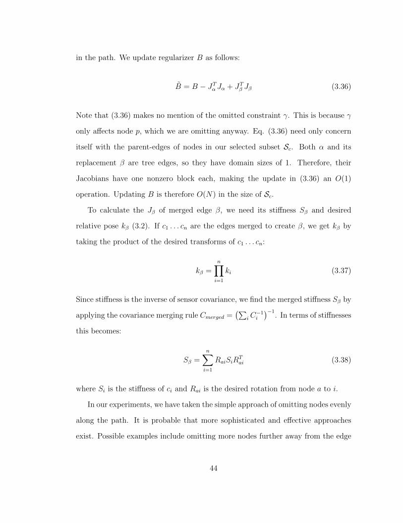
in the path. We update regularizer B as follows:

B = B − JTα Jα + JTβ Jβ (3.36)

Note that (3.36) makes no mention of the omitted constraint γ. This is because γ

only affects node p, which we are omitting anyway. Eq. (3.36) need only concern

itself with the parent-edges of nodes in our selected subset Sc. Both α and its

replacement β are tree edges, so they have domain sizes of 1. Therefore, their

Jacobians have one nonzero block each, making the update in (3.36) an O(1)

operation. Updating B is therefore O(N) in the size of Sc.

To calculate the Jβ of merged edge β, we need its stiffness Sβ and desired

relative pose kβ (3.2). If c1 . . . cn are the edges merged to create β, we get kβ by

taking the product of the desired transforms of c1 . . . cn:

kβ =n∏i=1

ki (3.37)

Since stiffness is the inverse of sensor covariance, we find the merged stiffness Sβ by

applying the covariance merging rule Cmerged =(∑

iC−1i

)−1. In terms of stiffnesses

this becomes:

Sβ =n∑i=1

RaiSiRTai (3.38)

where Si is the stiffness of ci and Rai is the desired rotation from node a to i.

In our experiments, we have taken the simple approach of omitting nodes evenly

along the path. It is probable that more sophisticated and effective approaches

exist. Possible examples include omitting more nodes further away from the edge

44

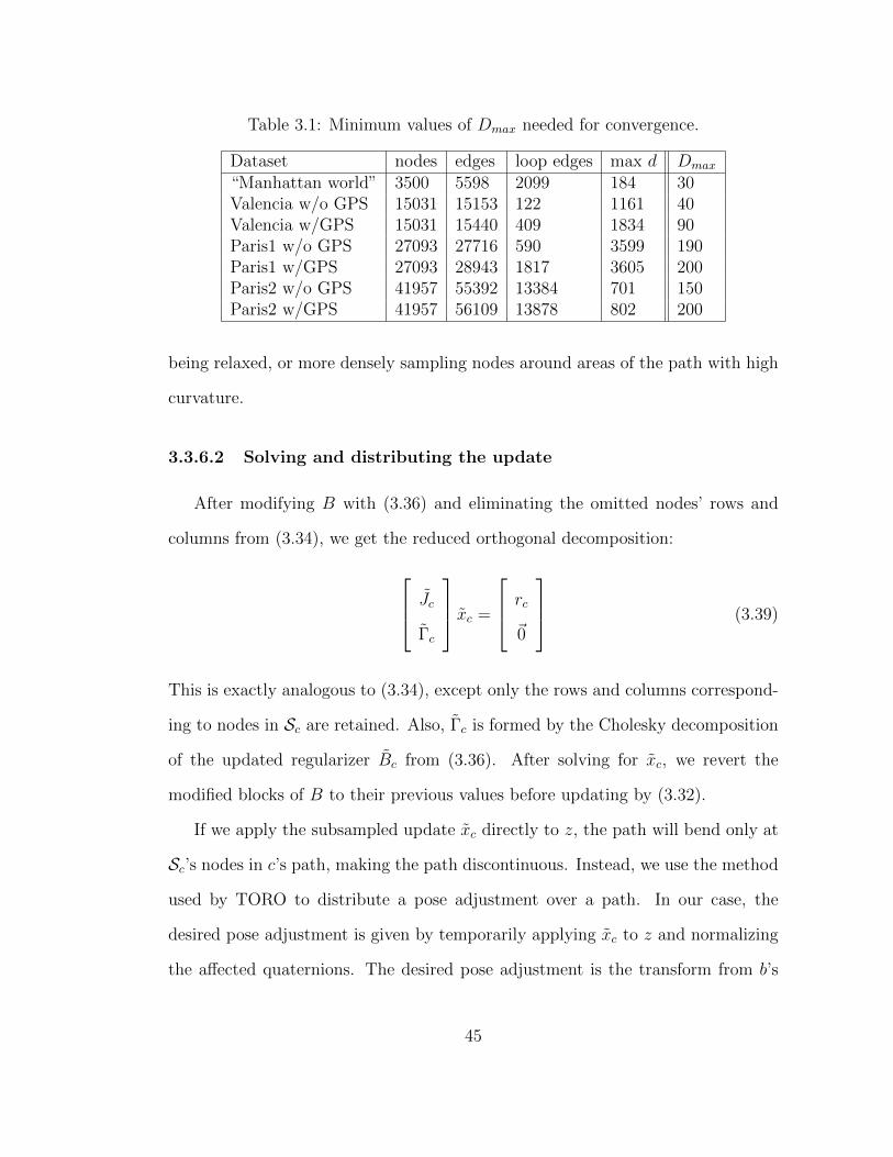
Table 3.1: Minimum values of Dmax needed for convergence.

Dataset nodes edges loop edges max d Dmax

“Manhattan world” 3500 5598 2099 184 30Valencia w/o GPS 15031 15153 122 1161 40Valencia w/GPS 15031 15440 409 1834 90Paris1 w/o GPS 27093 27716 590 3599 190Paris1 w/GPS 27093 28943 1817 3605 200Paris2 w/o GPS 41957 55392 13384 701 150Paris2 w/GPS 41957 56109 13878 802 200

being relaxed, or more densely sampling nodes around areas of the path with high

curvature.

3.3.6.2 Solving and distributing the update

After modifying B with (3.36) and eliminating the omitted nodes’ rows and

columns from (3.34), we get the reduced orthogonal decomposition:

Jc

Γc

xc =

rc

~0

(3.39)

This is exactly analogous to (3.34), except only the rows and columns correspond-

ing to nodes in Sc are retained. Also, Γc is formed by the Cholesky decomposition

of the updated regularizer Bc from (3.36). After solving for xc, we revert the

modified blocks of B to their previous values before updating by (3.32).

If we apply the subsampled update xc directly to z, the path will bend only at

Sc’s nodes in c’s path, making the path discontinuous. Instead, we use the method

used by TORO to distribute a pose adjustment over a path. In our case, the

desired pose adjustment is given by temporarily applying xc to z and normalizing

the affected quaternions. The desired pose adjustment is the transform from b’s

45

old pose to its new pose. We then distribute this adjustment over the nodes from

a down to b, not including a. As in TORO, we use the diagonal elements of B as

the distribution weights. For details on this distribution algorithm, we refer the

reader to [17]. This does not cause dog-legs, because xc updates rotations even for

position-only constraints.

3.3.7 Batch solving

It is possible to build a hybrid hessian HC for updating a set C of constraints

at once, by including the off-diagonal blocks of multiple constraints’ JTc Jc.

HC =∑c∈C

JTc Jc +BC (3.40)

Here the block-diagonal regularizer BC is formed from all edges not in C:

BC =∑i/∈C

B(JTi Ji) (3.41)

The equations to QR-factorize are then:

JC

ΓC

xc =

rC

~0

(3.42)

Here ΓC is created as before by the Cholesky decomposition BC = ΓTCΓC. We

form the batch-Jacobian JC and batch-residual rC by stacking the Jacobians and

residuals for edges in C, much as we did in (3.7) and (3.8).

We vertically stack Jc and rc corresponding to the constraints c in C to get JC

and rC. When C contains all the constraints in the posegraph, JC becomes J , and

46

ΓC vanishes, since there are no edges that are not in C (3.41). This reduces (3.42)

to the full exact update equation (3.17), yielding the exact update when solved.

3.3.8 Node and edge reordering

As pointed out by several authors [11, 27], the cost of solving for a batch-

update like xc depends greatly on the row and column ordering used in (3.42). In

offline√SAM [11] and SPA [31], this is done using approximate minimum degree

(AMD), a heuristic devised for general sparse problems [7]. Much work has been

done in finding good orderings for sparse QR factorizations, e.g. [20].

Unlike these methods, we usually solve for one edge at a time, resulting in

a matrix that is already so close to upper-triangular (3.35) that reordering its

columns will not improve efficiency. When we do batch-relax multiple edges, we

do so with a handful of GPS edges, for reasons described in section 3.3.10. GPS

edges have long paths that reach from the constrained node all the way up to the

Earth node at the root of tree. This leads to dense rows, which can limit the

usefulness of AMD [2]. We therefore use a simple, alternative approach that has

sufficed for our needs of relaxing a handful of constraints within real-time bounds.

The cost of upper-triangularizing the left-hand side of (3.42) increases sharply

with the number of sub-diagonal nonzeros. We therefore seek to permute the rows

and columns in a manner that keeps most nonzeros above the diagonal.

To illustrate, we show the extreme case of batching all edges together, i.e.

solving for the exact solution. Fig. 3.5 shows the block-sparsity pattern of the

total Jacobian J (3.7), constructed from all edges in Olson’s Manhattan dataset.

Each row is an edge Jacobian Je (3.6). Before reordering, these are stacked in

chronological order of their corresponding edges. Each column corresponds to

47

a node, again listed in chronological order of their nodes. We will first reorder

the nodes (columns), then the edges (rows). To do so, we first introduce some

terminology.

A node’s “edge count” is the number of edges whose Jacobians are affected

by that node. We may determine a node’s edge count by counting the number of

nonzero blocks in its corresponding column in JC. A “segment” is a chain of nodes

up the tree from child to parent. It starts from a branching node in the tree, and

stops just below the next branching node. All the nodes in a segment affect the

same set of edges, and therefore have the same edge count. We arbitrarily assign

unique ID numbers to each segment.

We sort the nodes (columns) primarily by increasing edge count, breaking ties

by segment ID, then by depth. By doing so, the columns (nodes) that affect the

same rows (edges) are grouped together, and columns that affect the most edges

are placed to the right of the matrix. This ordering is evident in fig. 3.5b, where

the densest columns can be seen grouped to the right.

Having sorted the columns, we now sort the edges by the index of the first

nonzero. This moves many of the nonzeros out of the lower triangle, leading to a

“semi-triangular” shape that is easier to upper-triangularize.

It is important to note that our method focuses on stochastic optimization,

with exact solving offered as an option to be used infrequently. Exact updates

with our method cost more than when performed using solvers designed for exact

updates only, such as iSAM [27]. This is because we use hierarchical poses, which

produce denser J matrices when all edges are batched together.

48

3.3.9 Online Tree Balancing

The worst-case cost of a new edge is O(d2t ), where dt is the maximum depth

in the tree. This happens when the new edge connects the deepest node in the

tree to another node, and their common ancestor is the root. To minimize this

worst-case cost, we must keep the tree depth dt small by maintaining a balanced

pose tree. In this section we describe our method for doing so.

Let e be a new edge connecting nodes a and b, with tree depths da and db. If db

is greater than da + 1, we may reduce it to da + 1 by making a the new parent of b.

Having reduced b’s depth, we must then recursively check its neighbors in the pose

graph to see if we may reduce their depths as well, by making b their parent. This

recursive tree restructuring can be done by performing a breadth-first traversal of

the graph from b, halting the recursion if no neighbor of the current node benefits

from becoming its child.

When an edge connects two separate pose graphs, their trees must be merged.

We do this by simply growing the larger graph’s spanning tree into the smaller

graph, using a breadth-first traversal starting from the connecting node.

When we give a node a new parent, this changes the path up the tree from

that node. This changes the domain of any edge whose domain contains that

node. For any such edge e, we must update its contribution JTe Je to regularizer

B =∑

iB(JTi Ji). This is a linear-time operation in the combined size of e’s old

and new domains.

By maintaining a balanced tree, we limit the tree depth to dt = O(logb(N)),

where b is the branching factor of the spanning tree. The worst case cost Cmax

is then Cmax = O(log2b (N)). As shown in section 3.3.6, interpolated solving can

further reduce this cost to being linear in the tree depth, giving a minimum bound

49

Algorithm 1 H2O

loopReceive new edge e from sensors.AddEdge(e) // See algorithm 2if e is a GPS edge thenG ← GetUpstreamGPSes(b, gps batch size)BatchUpdate(G, Dmax)

elseUpdate(e, Dmax)

end ifend loop

that is well within real-time limits for most pose graphs:

O(logb(N)) < Cmax < O(log2b (N)) (3.43)

Between these bounds, the actual cost can be chosen at run-time to match the

available CPU budget for that frame.

Algorithm 2 AddEdge

Input: New edge e, connecting nodes a and b.if neither a nor b are new then

Add e as a cross-edge.if a.depth > b.depth then

Swap(a, b)end ifif b.depth > a.depth + 1 then

Rebalance(e, b)end if

elseif a is new then

Swap(a, b)end ifAdd e as a tree edge, making b a child of a

end if

50

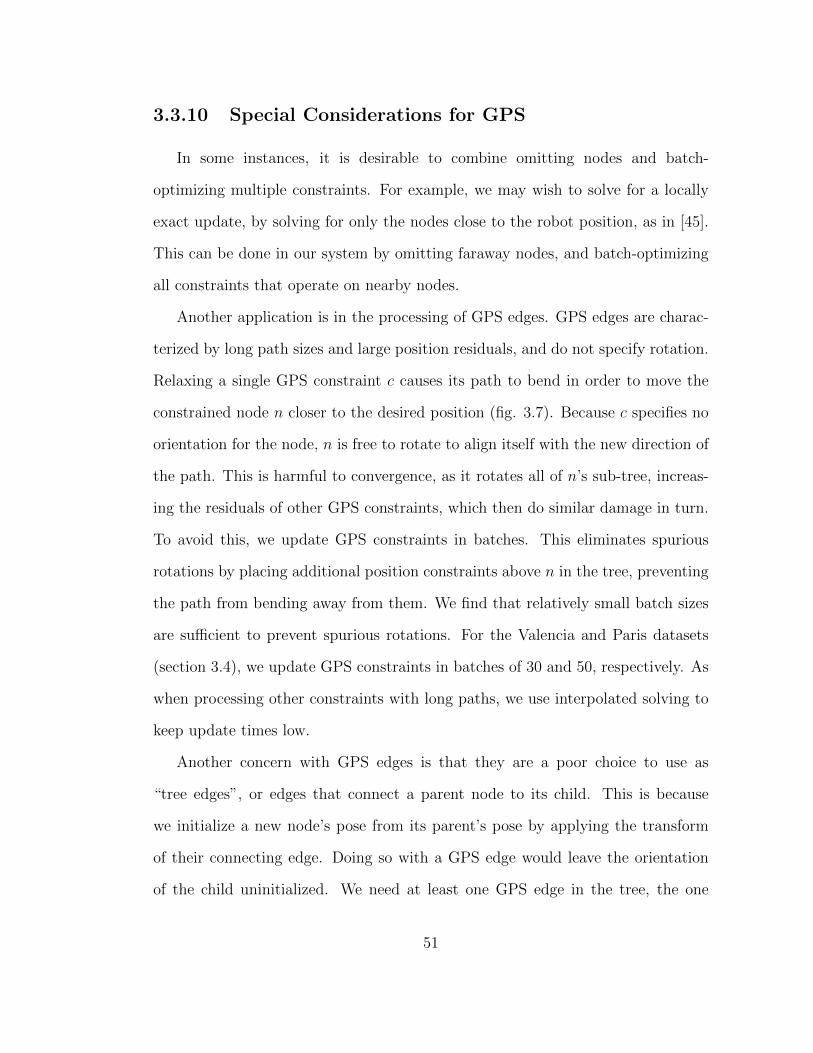
3.3.10 Special Considerations for GPS

In some instances, it is desirable to combine omitting nodes and batch-

optimizing multiple constraints. For example, we may wish to solve for a locally

exact update, by solving for only the nodes close to the robot position, as in [45].

This can be done in our system by omitting faraway nodes, and batch-optimizing

all constraints that operate on nearby nodes.

Another application is in the processing of GPS edges. GPS edges are charac-

terized by long path sizes and large position residuals, and do not specify rotation.

Relaxing a single GPS constraint c causes its path to bend in order to move the

constrained node n closer to the desired position (fig. 3.7). Because c specifies no

orientation for the node, n is free to rotate to align itself with the new direction of

the path. This is harmful to convergence, as it rotates all of n’s sub-tree, increas-

ing the residuals of other GPS constraints, which then do similar damage in turn.

To avoid this, we update GPS constraints in batches. This eliminates spurious

rotations by placing additional position constraints above n in the tree, preventing

the path from bending away from them. We find that relatively small batch sizes

are sufficient to prevent spurious rotations. For the Valencia and Paris datasets

(section 3.4), we update GPS constraints in batches of 30 and 50, respectively. As

when processing other constraints with long paths, we use interpolated solving to

keep update times low.

Another concern with GPS edges is that they are a poor choice to use as

“tree edges”, or edges that connect a parent node to its child. This is because

we initialize a new node’s pose from its parent’s pose by applying the transform

of their connecting edge. Doing so with a GPS edge would leave the orientation

of the child uninitialized. We need at least one GPS edge in the tree, the one

51

that connects the Earth at the root to the rest of the tree below it. The global

orientation of this subtree cannot be determined until we collect three GPS edges,

at which point we can initialize it to the orientation that provides the best fit.

Only after initializing the global orientation do we relax any GPS edges.

3.3.11 Temperature

To aid convergence, we scale update xc by a temperature parameter τ , before

adding it to parameters z as: z ← z + τxc. We start with τ = 1, and slowly

decrease it over time. We do this by scaling τ by 0.99 after each loop through all

constraints. If a constraint c’s residual is large, the resulting τxc may contain large

rotation updates, which can adversely affect convergence. For such updates, we

temporarily substitute τ for a value τ ′, which is chosen so that the largest rotation

update in τ ′xc does not exceed π/8.

3.3.12 Choosing edges

When run offline, we relax edges in increasing order of their edge roots. Because

relaxing an edge leaves all nodes above the edge root untouched, this ordering serves

to reduce oscillation, as relaxing each edge does not undo any work above it in the

tree. When performing multiple loops, the edges are looped through in this order.

When running online, the edges are relaxed in the order in which they are

added. Surplus CPU time may be spent revisiting old edges according to the

user’s priorities. A common strategy as employed in Sibley’s Relative Bundle

Adjustment [45], would be to re-relax local edges to emphasize local consistency.

52

3.3.13 Algorithm summary

We summarize our method in algorithm 1. The functions “Update” and

“BatchUpdate” implement single and multi-constraint updates as described above,

using interpolated solving to solve for no more than Dmax nodes at a time. The

“GetUpstreamGPSes(b, n)” function crawls up the tree from node b, and returns

the first n GPS edges along that path. In the AddEdge subroutine 2, “Rebalance”

is the recursive tree-balancing operation described in section 3.3.9. For simplic-

ity, we have omitted from AddEdge the fact that we replace GPS tree edges with

non-GPS edges whenever possible, for reasons described in 3.3.10.

3.4 Results

In this section we report H2O’s performance in the 2011 RSS/WillowGarage

SLAM evaluation workshop, demonstrate its convergence on maps from commonly

used datasets and Google’s Street View database, show the effect of subsampling

on convergence quality, and show its robustness to noisy sensor input.

3.4.1 RSS/WillowGarage Automated SLAM Evaluation

Workshop results

This algorithm was submitted to the Automated SLAM Evaluation Workshop,

held at RSS 2011. On their four benchmark datasets, it competed against other

approximate SLAM algorithms HOG-Man [16] and SLoM [21]. It outperformed

them in time and χ2-error on the two 3D datasets, and tied for first place with

SLoM overall. We used a maximum domain size Dmax of 200, and no edge batching.

53

Full contest details and results may be seen at [26].

3.4.2 Relaxing pose graphs

Fig. 3.8 shows a section of our “Paris1” posegraph before and after optimiza-

tion, both with and without GPS constraints. We show a case where, without

GPS constraints, the optimization causes rotations at an under-constrained inter-

section, causing the loop to rotate into an unrealistic configuration. We show that

GPS constraints serve to limit such error. We also show an instance of the dog-leg

problem experienced by TORO. Even though the dog-leg problem is typical with

GPS constraints, it can also happen, as it did here, with loop-closing constraints

that have a large position residual and small rotation residual. Our method does

not suffer from this problem.

In fig. 3.9, we show some maps before and after solving with our method.

The “before” images show the poses as initialized by starting at the root of the

parametrization tree, and crawling downwards, concatenating the tree edges’ trans-

forms. For a pose graph with no loop closures, this would be equivalent to dead-

reckoning. The red edges are edge residuals, connecting the desired pose of a

node to its actual pose. Relative constraints’ residuals connect two poses, while

GPS constraints’ residuals connect a pose to a spot in empty space, indicating the

desired position. Redder residuals indicate higher error. Longer residuals do not

necessarily have higher error, as some edges are less stiff than others. In particular,

GPS constraints are much less stiff than other types, due to GPS’ imprecision. Our

method performs well on graphs with ample loop closures, such as Olson’s “Man-

hattan world”, converging to an average energy per constraint of 1.596, compared

to TORO’s 2.062. Our method completely collapses most relative constraint resid-

54

uals (fig. 3.9b, 3.9d), and greatly reduces GPS residuals (fig. 3.9f). A small number

of lines which overlap in fig. 3.9e can be seen to have split apart in 3.9f. These

are parallel runs where the loop closure detector failed to recognize as traversing

the same path, and therefore did not connect together with a constraint. Outdoor

urban maps can have fewer loop-closures, due to the difficulty of detecting them

in highly dynamic environments. Despite this distortion, the solved map aligns

relatively well to satellite photography, as seen in fig. 3.10.

3.4.3 Convergence

In fig. 3.11, we show the log-energy per constraint over time for our method

and TORO. Our method reduces the error quicker, and converges to an average

energy per constraint that is an order of magnitude lower than that of TORO.

For our method, we use interpolated solving as described in section 3.3.6, with

different maximum values Dmax for the size of set Sc. GPS constraints were not

used, to minimize dog-legs in TORO. The pose graph data was taken from a

section of Valencia, Spain, with 15031 poses and 15153 constraints. The energy

was measured after each loop through all constraints. In actual operation, only a

few constraints are added or updated per frame, so the spacing of the points in

the plot should not be interpreted as the required time per iteration. Rather, see

table 3.2 for the average and maximum time per constraint for the same solvers

and posegraph. The average constraint domain size was 1.53 poses, while the

largest constraint domain was 1161 poses. The times shown are all within real-

time bounds per frame, except when domain subsampling is turned off (by setting

Dmax =∞).

Linearizing the relation between position error and rotation updates is neces-

55

Table 3.2: Average and maximum time per constraint, Valencia dataset

Solver Avg. time (s) Max. time (s)TORO 1.75092 ∗ 10−5 5.24759 ∗ 10−3

Dmax = 75 3.6635 ∗ 10−4 5.3559 ∗ 10−2

Dmax = 100 4.0791 ∗ 10−4 6.5095 ∗ 10−2

Dmax = 150 4.919 ∗ 10−4 9.5015 ∗ 10−2

Dmax = 200 5.812 ∗ 10−4 0.13747Dmax =∞ 2.0823 ∗ 10−3 3.583

sary for properly addressing the dog-leg problem. However, such projective rota-

tions can also cause oscillations in the face of excessive subsampling. To test our

method’s robustness to oscillations, we ran the solver with various levels of sub-

sampling, defined by Dmax, the maximum number of nodes to solve for in (3.39).

Table 3.1 shows the minimum values of Dmax which did not cause divergence. Note

that these are not hard minimums, as divergence may also be avoided by lowering

the initial temperature τ from 1.0. This table is only intended to illustrate the

potential danger of over-subsampling. Table 3.1 also shows each map’s number

of nodes, edges, loop edges, and maximum domain size (“max d”). Loop edges

are edges with more than two nodes in their path (they are also counted under

“edges”). The “Manhattan world” dataset was originally used by Olson in [38]

(see fig. 3.9a).

In fig. 3.11, we compare online and offline operation of H2O. The first iteration

of the online hybrid hessian run is delayed (shifted to the right) due to the overhead

incurred by the dynamic tree balancing described in section 3.3.9.

3.4.4 Robustness to noise

To test the robustness of our solver to large errors due to sensor noise, we

added rotational noise to all edges in the “Manhattan world”, Valencia, and Paris2

56

pose graphs. These “noisified” graphs can be seen in fig. 3.12. Each rotation was

multiplied by a small rotation around the local up axis, where the angle was drawn

from a normal distribution with a standard deviation of 3 degrees. When the poses

are initialized using these edges, these small rotations add up to the large map

distortions shown in the left column.

3.5 Conclusions and Future Work

We have described a method for online SLAM which combines strengths from

stochastic and exact approaches, and provides a means of controlling the exactness

and cost of a given SLAM update. Like previous stochastic methods, our method

exhibits fast-converging updates and robustness to large initialization errors. Like

exact methods, we are able to process GPS constraints without introducing the

pose staggering known as the “dog-leg problem”, previously a weakness of stochas-

tic methods. We demonstrated a means of reducing the complexity of updates in

order to stay within real-time bounds on every update, so as not to disrupt higher-

level operations with cost spikes. In addition, we demonstrated batch-optimizing

multiple constraints, with applications to stable GPS updates. Taken together,

these techniques allow the user to smoothly transition between approximate O(n)-

per-constraint loop closing (where n is the size of the constraint’s loop), and exact

updates as used by exact solvers. Our algorithm optimizes to a lower overall en-

ergy than a state-of-the-art method in stochastic SLAM, while staying well within

real-time cost bounds per constraint. We have presented a means of dynamically

balancing a parametrization tree to minimize the worst-case cost of future loop-

closures. Finally, we demonstrated a simple scheme of row and column ordering

57

to ease batch-solving multiple constraints.

In the future, we would like to investigate using spare CPU time to relax old

edges. How to select which edge to revisit, and how to minimize disruptions to

its nodes’ subtrees, remain open questions. To that end, a remaining problem

with our method is that old nodes higher up in the pose tree become resistant to

change, as newer edges add to those nodes’ corresponding values in the regularizer

B. This can make relaxing old sections of the pose graph resistant to change.

Further investigation is necessary to selectively “un-stiffen” parts of the old graph

in response to new information.

Reordering the columns and rows when batch-relaxing edges is another topic

with room for exploration. Our tree parametrization results in groups of rows with

similar sparsity patterns, making them amenable to supernodal approaches to QR

factorization [8].

58

0 1000 2000 30000

1000

2000

3000

4000

5000

(a) J matrix

0 1000 2000 30000

1000

2000

3000

4000

5000

(b) J , reordered

Figure 3.5: Reordering edges and nodes: The sparsity pattern of the full square-root information matrix (J) of the Manhattan dataset [37], constructed from all of theedges. Each column corresponds to a node (pose), while each row corresponds to anedge (sensor reading). In fig. 3.5a, the rows and columns are listed in chronologicalorder of their corresponding sensor readings and poses. In fig. 3.5b, they are sorted asdescribed in section 3.3.8. This matrix has fewer sub-diagonal elements, making it easierto upper-triangularize and solve. The left matrix took 41.52 seconds to QR-factorizewith Householder reflections on a 2 GHz Intel Core 2 Duo; the right matrix took 12.26seconds.

59

(a) Pose graph (2500 nodes) (b) Naive tree (dmax = 2500)

(c) BFT (offline, dmax = 50) (d) Online balancing (dmax = 50)

Figure 3.6: Online tree balancing. From left to right: fig. 3.6a shows the spheredataset [17], a pose graph formed by a robot spiraling down a sphere from top to bottom.The remaining figures show various spanning trees, where tree depth is indicated by color(redder is deeper). Figure 3.6b shows a pathological case of naive tree growth, in whichold nodes never change parents. Online TORO and SGD use this method. Fig. 3.6cshows a tree built offline by simple breadth-first traversal of the graph, as employed in[15]. This guarantees a balanced tree, but can only be done offline, not online. Fig. 3.6dshows the tree when using dynamic balancing, as described in section 3.3.9.

60

(a) Two GPS constraints

(b) Relaxing them sequentially

(c) Batch-relaxing them together

Figure 3.7: Batch-relaxing GPS Because GPS constraints do not specify rotation,relaxing them one at a time can cause spurious rotations of the constrained node and itssubtree. To lock down rotation, we relax them together in a batch.

61

(a) Initial pose tree, detail (b) After convergence

(c) Underconstrained loop (d) Same loop with GPS

(e) Dog-legged path, after convergencewith TORO

(f) Same path, after convergence with ourmethod

Figure 3.8: Paris1 dataset A posegraph taken from a section of Paris, with 27093nodes and 27716 constraints. Fig. 3.8a shows a section of the pose tree in its initialstate. Stretched constraints can be seen as red lines. Fig. 3.8b is the same section after10 iterations of our method, using a maximum problem size of Dmax = 200, and noGPS constraints. The stretched constraints of 3.8a have collapsed; the runs that remainseparated are those without constraints tying them together. Fig. 3.8c shows a severelyunder-constrained intersection, with few loop-closing constraints connecting adjacentruns. Such intersections can happen due to the difficulty in identifying loop closures indynamic urban environments. While optimizing the posegraph, parallel paths with nocross-connections can become separated. Fig. 3.8d shows the same intersection whenGPS constraints are added to one out of every 100 nodes. The GPS’ residual vectors arevisible as blue line segments. Unlike loop-closing constraints, GPS constraints are easyto come by, limit drift in large loops, and prevent separation of nearby unconnected runs.Fig. 3.8e shows a portion of the Paris posegraph after convergence with TORO. Thedog-leg problem has caused the vehicle poses to not point along the direction of travel.No GPS constraints were used. Fig. 3.8f shows the same portion, after convergence withour method.

62

(a) Olson’s “Manhattan world” (b) “Manhattan world”, converged

(c) Valencia (d) Valencia, converged

(e) Paris2 (f) Paris2, converged

Figure 3.9: Solved maps Pose graphs, before and after 10 iterations with Dmax = 200.Pose graph sizes are given in table 3.1. Initial configurations show the poses as setby concatenating constraint transforms down the tree, as described in section 3.3.2.Constraint residuals are shown as brown/red lines connecting the constraint’s desiredpose to the actual pose. Brighter red indicates higher error. Valencia (fig. 3.9c, fig.3.9d) is shown at an oblique angle, to better show its error residuals, which are primarilyvertical.

63

Figure 3.10: Montmartre, Paris An overlay of the converged poses of fig. 3.9f on asatellite image from Google Earth.

64

0 10 20 30 40 50 60Time (seconds)

10-3

10-2

10-1

100

101

Log(a

vera

ge e

nerg

y p

er

constr

ain

t)

hh, offline

hh, online

toro, offline

Figure 3.11: Online vs offline convergence Online tree-balancing incurs some ad-

ditional cost over offline operation, as shown by the rightward shift of the green line

(online) relative to the blue line (offline). Each point represents a complete loop through

all edges. After the first loop, the online algorithm revisits old edges in depth-first order.

65

(a) “Manhattan world”, noisified (b) “Manhattan world”, converged

(c) Valencia, noisified (d) Valencia, converged

(e) Paris2, noisified (f) Paris2, converged

Figure 3.12: Graphs with large initial error Pose graphs, with noisified constraints(sensor readings). A small random rotation around the local up axis was multiplied ontoeach constraint’s rotation, causing large distortions to accumulate over time. Pose graphsizes given in table 3.1. Constraint residuals are shown as brown/red lines (redder =more error).

66

4Conclusions and Future Work

SLAM solvers have rightly aspired to be a black box: a general purpose tool

that offers few controls, and in turn asks few questions of the work to which it is

put. Unfortunately, making localizers insensitive to their context can make them

much more expensive than necessary. The efficiency loss can be great enough to

impact the overall capability of the robot. In chapter 2, it made the difference

between being able to afford a long-distance vision module, or not. In chapter 3,

it determined whether SLAM could guarantee real-time operation, or not. When

67

the expense of a black box affects high-level design decisions, it is no longer a black

box.

In localization, speed and accuracy are competing priorities. Many localizers

seek to distinguish themselves by optimizing for one or the other. This thesis

argues that a localizer should instead position itself between these priorities in a

way that best serves the task at hand.

Chapter 2 showed that by combining wheel odometry and visual odometry, one

may achieve comparable accuracy to pure visual odometry at 5 percent of the cost.

Hybridizing the two odometry types eliminates their biggest problems, namely

hallucinated rotations caused by wheel slip, and processor saturation caused by

the high cost of pure visual odometry.

Chapter 3 described H2O, a SLAM solver which can dynamically adjust be-

tween exact accuracy and fast linear-time speed. This provides a unique control

knob. It allows the robot to dictate the computational budget of SLAM, rather

than the other way around. This enables SLAM to remain unobtrusive to the rest

of the robot’s system, as a black box should. At its fastest and least accurate set-

ting, our solver converges faster than the fastest competing SLAM solver, with a

χ2-error that is lower by a factor of 10. At its most accurate setting, H2O matches

the error of exact SLAM solvers.

There is room to improve H2O along its two primary strengths: cost, and

flexibility. H2O already boasts very fast loop-closing times, but pushing the speed

too far can harm convergence. This limit is currently determined empirically. We

expect that with further study, we will be able to determine this limit for a loop

before actually solving it, thus enabling us to make loop closures as fast as is

sensible, but no faster. Another strength of H2O is its flexibility: the user may

68

choose which poses and edges to solve for. This allows for useful optimizations,

such as solving only for poses close to the robot, for example. While useful, such

arbitrary relaxations are more likely to introduce discontinuities in the map, as

compared to the default usage of relaxing the most recently added edge. Studying

how to prevent such discontinuities, and how to most efficiently repair them when

they occur, will further enhance H2O’s flexibility.

69

ADifferentiating Hierarchical Poses

Hierarchical trees of rigid-body transforms find use in many problems, such as

inverse kinematics, segmented limb control, and as seen in this thesis, SLAM. Such

problems often optimize some error function of pose, requiring us to differentiate

this pose with respect to the chain of transforms from which it is formed. Resources

that describe the necessary calculus in sufficient detail remain surprisingly hard to

find. This appendix presents a complete derivation, for the benefit of implementors.

70

Notation

In this section, we consider a chain of tranforms from node 0 (the root of the

pose tree) down to a node N , using the following conventions and symbols.

Conventions

• All vectors are column vectors.

• Quaternions are laid out as [ w x y z ].

• If x = [ x1 · · · xm ] and y = [ y1 · · · yn ], the derivative ∂x∂y

is a m× n

matrix where the element at row r and column c stores ∂xr∂yc

.

• Given a quaternion q and 3-D vector v, the notation qv expresses a quaternion

product between q and the quaternion [ 0 v ].

Symbols

tn, qn Relative translation and rotation quaternion from pose n-1 to n.

xn, rn Global position and rotation quaternion of pose n (A.3).

Qn, Rn Rotation matrix representation of quaternions qn, rn (A.5).

f(v, q) Vector v, rotated by quaternion q. Defined as qvq−1, equal to Qv.

qI , I Identity quaternion [ 1 0 0 0 ], and the identity 3× 3 matrix.

Mq Quaternion q, treated as a vector, multiplied with matrix M .

M ⊗ q Quaternion-multiplication of the columns ofM , with q (A.1, A.2).

Let M be a 4× 4 matrix. Writing M ’s columns as M =

[c0 c1 c2 c3

], we

71

define ⊗ using columnwise quaternion multiplication:

M ⊗ q =

[c0q c1q c2q c3q

](A.1)

q ⊗M =

[qc0 qc1 qc2 qc3

](A.2)

Kinematic chain notation

There are various notational conventions for chaining rigid body transforma-

tions. We illustrate ours by spelling out the expressions for global poses 0 through

3:

r0 = q0 x0 = t0

r1 = q0q1 x1 = t0 + f(t1, q0)

r2 = q0q1q2 x2 = t0 + f(t1, q0) + f(t2, q0q1)

r3 = q0q1q2q3 x3 = t0 + f(t1, q0) + f(t2, q0q1) + f(t3, q0q1q2)

If we define r−1 to be the identity rotation, we may write the n’th global pose as:

rn =n∏i=0

qi (A.3)

xn =n∑i=0

f(ti, ri−1) (A.4)

72

or using matrix notation:

Rn =n∏i=0

Qi (A.5)

xn =n∑i=0

Ri−1ti (A.6)

Differentiating Global Poses

We wish to modify the local transforms to minimize some convex error function

E(xn, rn) of the global pose at the end of the chain. We start by taking the

gradients with respect to ti and qi :

∂E

∂ti=∂E

∂xn

∂xn∂ti

+∂E

∂rn7

0∂rn∂ti

(A.7)

∂E

∂qi=∂E

∂xn

∂xn∂qi

+∂E

∂rn

∂rn∂qi

(A.8)

We note from (A.3) that the Jacobian ∂rn∂ti

is zero, hence its cancellation in (A.7)

above. The remainder of this section will derive the remaining Jacobians ∂xn∂ti

, ∂xn∂qi

,

and ∂rn∂qi

.

Global position with respect to local translation

The Jacobian with respect to the local translation ti is simple. Differentiating

both sides of (A.6), all but the i’th term in the sum drop out to yield:

∂xn∂ti

= Ri−1∂ti∂ti

(A.9)

= Ri−1I (A.10)

73

Thus:

∂xn∂ti

= Ri−1 (A.11)

As one might expect, this shows that variations of ti can be mapped to varia-

tions of xn by Ri−1, the global orientation of the pose just above ti in the kinematic

chain.

Global position with respect to local rotation

The Jacobian of global position xn with respect to the local rotation qi is more

involved. In fact, we will show that it is more convenient to derive the Jacobian in

a rotated coordinate frame where qi = qI . We will then use this Jacobian to update

the transformed qi, then transform the updated qi back to its original coordinate

frame.

We start by differentiating both sides of (A.6):

∂xn∂qi

=∂

∂qi

n∑j=0

Rj−1tj (A.12)

74

We can drop all terms in the sum that do not contain qi to get:

∂xn∂qi

=∂

∂qi

n∑j=i+1

Rj−1tj (A.13)

=n∑

j=i+1

∂

∂qiRj−1tj (A.14)

=n∑

j=i+1

∂

∂qi

(j−1∏k=0

Qk

)tj (A.15)

=n∑

j=i+1

(i−1∏k=0

Qk

)∂

∂qi

(j−1∏l=i

Ql

)tj (A.16)

=n∑

j=i+1

Ri−1∂

∂qi

(j−1∏l=i

Ql

)tj (A.17)

According to Wheeler and Ikeuchi [53], the Jacobian of a rotated vector f(v, q)

with respect to the rotating quaternion q takes a particularly simple form when

q = qI , the identity:

∂f(v, q)

∂q

∣∣∣∣q=qI

=

0 0 2z −2y

0 −2z 0 2x

0 2y −2x 0

(A.18)

where

[ x y z ] = f(v, q) (A.19)

This handy fact can be applied to any value of q and v, by rotating them into a

75

frame where q = qI :

v′ = f(v, q) (A.20)

q′ = qI (A.21)

In (A.17), we perform a similar change of variables from tj and qi:

t′j =

(j−1∏l=i

Ql

)tj (A.22)

q′i = qI (A.23)

This yields an expression for ∂xn∂q′i

:

∂xn∂q′i

=n∑

j=i+1

Ri−1

∂t′j∂q′i

(A.24)

Where∂t′j∂q′i

is given by plugging in [t′j = x y z ] into (A.18).

Given the Jacobian ∂xn∂q′i

, we can solve for a step ∆q′i for q′i using whatever

gradient-based nonlinear optimization algorithm we choose. The linearized update

to q′i is:

q′i ← (q′i + ∆q′i)/||q′i + ∆q′i|| (A.25)

Note the normalization, done to ensure that q′i remains a pure rotation with no

scaling. To transform the updated q′i back to the original unrotated coordinate

frame qi, we use the definition:

qi = qcq′i (A.26)

Here qc is the value of qi before the update step.

76

Finally, we pause to note one feature of the Jacobian ∂v′

∂q′given by (A.18),

namely that its first column is all zeros. This column corresponds to variations

in the first element of q′. Intuitively, this means that any gradient descent step

∆q′ that simply scales the current value of q′ = [ 1 0 0 0 ] without changing

the rotation it represents will have no effect on f(v′, q′). Conversely, using this

Jacobian to calculate a step ∆q′ will not move q in such useless directions. This

relieves us of having to impose extra constraints, such as Lagrange multipliers, on

q′. We do still need to normalize q′ after the update, as q′ + ∆q′ may not be unit

length.

Global rotation with respect to local translation

By inspection of (A.3), we see that global rotation does not depend on local

translation:

∂rn∂ti

=

0 0 0

0 0 0

0 0 0

0 0 0

(A.27)

Global rotation with respect to local rotation

Global rotation rn is a product of a chain of local rotations:

rn =n∏j=0

qj From (A.3) (A.28)

We would like to differentiate rn with respect to one of these local rotations, qi.

We start by multiplying together all rotations above qi in the chain, and similarly,

77

all rotations below qi. We call these products qa and qb:

rn =

(i−1∏j=0

qj

)qi

(n∏

k=i+1

qk

)(A.29)

= qaqiqb (A.30)

Differentiating (A.30) with respect to qi, we get:

∂rn∂qi

= qa ⊗ I ⊗ qb (A.31)

where I is a 4× 4 identity matrix, and we use ⊗ to denote columnwise quaternion

multiplication. In other words, the c’th column of ∂rn∂qi

is the quaternion product

qaIcqb, where Ic is the c’th column of I.

If we are to use this ∂rn/∂qi alongside ∂xn/∂q′i from section A, we need to

modify it to use the transformed rotations q′i rather than qi. This is easily done by

plugging qi = qcq′i (A.26) into (A.29):

rn =

(i−1∏j=0

qj

)qi

(n∏

k=i+1

qk

)(A.32)

=

(i∏

j=0

qj

)q′i

(n∏

k=i+1

qk

)(A.33)

= q′aq′iqc (A.34)

78

where

q′a =

(i∏

j=0

qj

)(A.35)

q′i = qI (A.36)

As with (A.31), we differentiate both sides of (A.34) to get:

∂rn∂q′i

= q′a ⊗ I ⊗ qb (A.37)

Differentiating Relative Poses

Instead of minimizing an energy function of a global pose, we may want to

minimize an energy function of the relative pose between two global poses [xa, ra]

and [xb, rb]. In this section we differentiate this relative transform [tab, qab] with

respect to the hierarchical transforms [ti, qi].

While the following equations are written in terms of “global poses” [xi, ri],

there is no special requirement that the poses be in the coordinate frame of the

pose tree’s root. Any consistent reference frame will yield the same results. In

practice, we use the reference frame of lowest common ancestor of poses a and b

in the pose tree.

79

Relative translation with respect to local translation

The relative translation tab is given by:

tab = f(xb − xa, r−1a ) (A.38)

= R−1a (xb − xa) (A.39)

Differentiating both sides with respect to ti gets:

∂tab∂ti

= R−1a

(∂xb∂ti− ∂xa∂ti

)(A.40)

The derivatives ∂xb∂ti

and ∂xa∂ti

are given by (A.11). We treat R−1a as a constant in

the above differentiation, since global rotations are independent of local transla-

tions (A.5).

Relative translation with respect to local rotation

Differentiating the relative translation tab (A.38) with respect to the local ro-

tation q′i yields:

∂tab∂q′i

=∂

∂q′if(xb − xa, r−1

a ) (A.41)

=∂

∂q′ira(xb − xa)r−1

a (A.42)

=∂ra∂q′i⊗ (xb − xa)r−1

a

+ ra ⊗(∂xb∂q′i− ∂xa∂q′i

)⊗ r−1

a

+ ra(xb − xa)⊗∂r−1

a

∂q′i

(A.43)

80

Expanding the ∂r−1a /∂q′i in the last term above gets:

∂r−1a

∂q′i=∂r−1

a

∂ra

∂ra∂q′i

(A.44)

=∂r∗a∂ra

∂ra∂q′i

r−1 = r∗ because r is unit length (A.45)

= I∗∂ra∂q′i

(A.46)

where

I∗ =

1 0 0 0

0 −1 0 0

0 0 −1 0

0 0 0 −1

(A.47)

Therefore:∂tab∂q′i

=∂ra∂q′i⊗ (xb − xa)r−1

a

+ ra ⊗(∂xb∂q′i− ∂xa∂q′i

)⊗ r−1

a

+ ra(xb − xa)⊗ I∗∂ra∂q′i

(A.48)

The ∂rn∂q′i

derivative is given by (A.37), while ∂xb∂ti

and ∂xa∂ti

are given by (A.11).

The(∂xb∂q′i− ∂xa

∂q′i

)term is a 3 × 4 matrix, whose 3-D columns are multiplied by

quaternions ra and r−1a . As when quaternion-multiplying 3-D position vectors,

this is done by padding the columns with leading zeros. The product is a 4 × 4

matrix with zeros in the first row. The remaining two terms above have first

rows which cancel out to zero when added together. The entire right-hand side

therefore resolves to a 4×4 matrix with a zero first row. The remaining three rows

are written to the left-hand side, the 3× 4 matrix ∂tab∂q′i

.

81

Relative rotation with respect to local translation

The relative rotation between global poses [xa, ra] and [xb, rb] is given by:

qab = r−1a rb (A.49)

As when deriving ∂r/∂t, we note from (A.3) that the global rotations ra and rb

are independent from local translations ti. Therefore,

∂qab∂ti

=

0 0 0

0 0 0

0 0 0

0 0 0

(A.50)

Relative rotation with respect to local rotation

Differentiating both sides of A.49 we get:

∂qab∂q′i

=∂r−1

a

∂q′i⊗ rb + r−1

a ⊗∂rb∂q′i

(A.51)

=∂r−1

a

∂ra

∂ra∂q′i⊗ rb + r−1

a ⊗∂rb∂q′i

(A.52)

Plugging in ∂r−1a

∂ra= I∗ (A.47) we get:

∂qab∂q′i

= I∗∂ra∂q′i⊗ rb + r−1

a ⊗∂rb∂q′i

(A.53)

where the ∂r∂q′

terms are given by (A.37).

82

BConstraint Jacobians

Here we show how to calculate the jacobians of arbitrary sensor types, so that

they may be used in graphical SLAM methods, such as the H2O algorithm of

chapter 3.

83

Constraint functions

Most graphical SLAM methods, including H2O, model edges as quadratic

penalty functions between an observed value k and a prediction function g(z),

which predicts the expected observed value, given state z:

E = ||g(z)− k| |Ω (B.1)

= (g(z)− k)TΩ−1(g(z)− k) (B.2)

This is the chi-squared error, or Mahalanobis distance, between the expected and

actual observations. It may be interpreted as the log-probability of P (k|z), where

P (k|z) is taken to be a Gaussian with mean g(z) and covariance Ω.

To incorporate these constraints into SLAM, we must know their Jacobian

and residual. In this appendix, we enumerate these for various types of sensors,

under the assumption that our parameters z store the relative transforms in a pose

tree 3.2, as in chapter 3. If z stores poses in a global refrence frame instead, the

jacobians are far simpler, and therefore left to the reader to derive.

Weighted jacobians and residuals

As described in 3.3.3, we may split Ω−1 into a lower triangular matrix L and

its transpose:

Ω−1 = LLT (B.3)

This allows us to express E not as a Mahalanobis distance, but as a simple norm

of a weighted residual:

E =∥∥LT (g(z)− k)

∥∥ (B.4)

84

As in chapter 3, we use the terms “Jacobian” and “residual” to refer to the weighted

Jacobian J and weighted residual r, defined as:

J = LT∂g(z)

∂z(B.5)

r = LT (g(z)− k) (B.6)

These may be plugged into (3.7), (3.8), and (3.14) to solve for an exact SLAM

update, or into (3.35) for a stochastic H2O update. In the remainder of this

appendix, we present the g(z) and k for all major sensor types, so that they may

be used in graphical SLAM.

Position sensors

For position sensors, g(z) calculates some absolute or relative position x, and

k is its measured value. The derivative ∂x∂z

is a 3× 7N matrix:

∂x

∂z=

[∂x∂t1

∂x∂q′1

∂x∂t2

∂x∂q′2

· · · ∂x∂tN

∂x∂q′N

](B.7)

The Jacobian J is also a 3× 7N matrix, and the residual r is a 3-D vector:

J = LT[

∂x∂t1

∂x∂q′1

∂x∂t2

∂x∂q′2

· · · ∂x∂tN

∂x∂q′N

]r = LT (x− k)

(B.8)

If x is a global position, it may be calculated from z using (A.4), and its derivatives

∂x∂ti

and ∂x∂q′i

are given by (A.11) and (A.24), respectively.

If x is a relative position, we calculate it using (A.38), and its derivatives its

85

derivatives ∂x∂ti

and ∂x∂q′i

are given by (A.40) and (A.48).

Orientation sensors

Because rotations do not occupy a cartesian space, some care is needed to fit

them into our cartesian penalty function g(z)−k. Let r(z) be an absolute (A.3) or

relative rotation (A.49) as calculated from parameters z, and rk the same rotation

as measured by a sensor. We then let:

E =∥∥±r(z)−1rk − qI

∥∥Ω

(B.9)

where qI is the identity quaternion [ 1 0 0 0 ]. In other words, we take the

rotation from the calculated orientation q(z) to the measured orientation rk, and

penalize its cartesian distance from the null rotation qI . This defines g(z) and k

as:

g(z) = ±r(z)−1rk (B.10)

k = I (B.11)

The derivative of g(z) is:

∂g(z)

∂z= ±∂r

−1

∂z⊗ rk (B.12)

= ±∂r−1

∂r

∂r

∂z⊗ rk (B.13)

= ±I∗ ∂r∂z⊗ rk (B.14)

86

Plugging (B.11) into (B.6), we get:

r = LTk (B.15)

= LT I (B.16)

Therefore

J = ±LT I∗[

∂r∂t1

∂r∂q′1

∂r∂t2

∂r∂q′2

· · · ∂r∂tN

∂r∂q′N

]⊗ rk

r = LT(B.17)

The ∂r∂ti

terms are filled with zeros, as per (A.27). If r is a global rotation, the ∂r∂q′i

derivatives are given by (A.37). If r is a relative rotation, the ∂r∂q′i

derivatives are

given by (A.53).

Pose sensors

Most sensors used in SLAM give a measure of relative pose, including both

the translation and rotaiton. For example, IMU and wheel odometry measure the

transform between two consecutive poses, while laser scan-matching and visual

feature matching give the transform between two poses with shared observations.

For such sensors, g(z) and k are 7-dimensional, with 3 dimensions for position and

4 for rotation. Their position and rotation components are given by the g(z)’s and

k’s for position and rotation sensors, described above. If position and orientation

are correlated, this may be expressed in the off-diagonal elements of the 7 × 7

cvariance matrix Ω. If some components of the pose are left underspecified by

the sensor (such as vertical translation for wheel odometry), this can be expressed

87

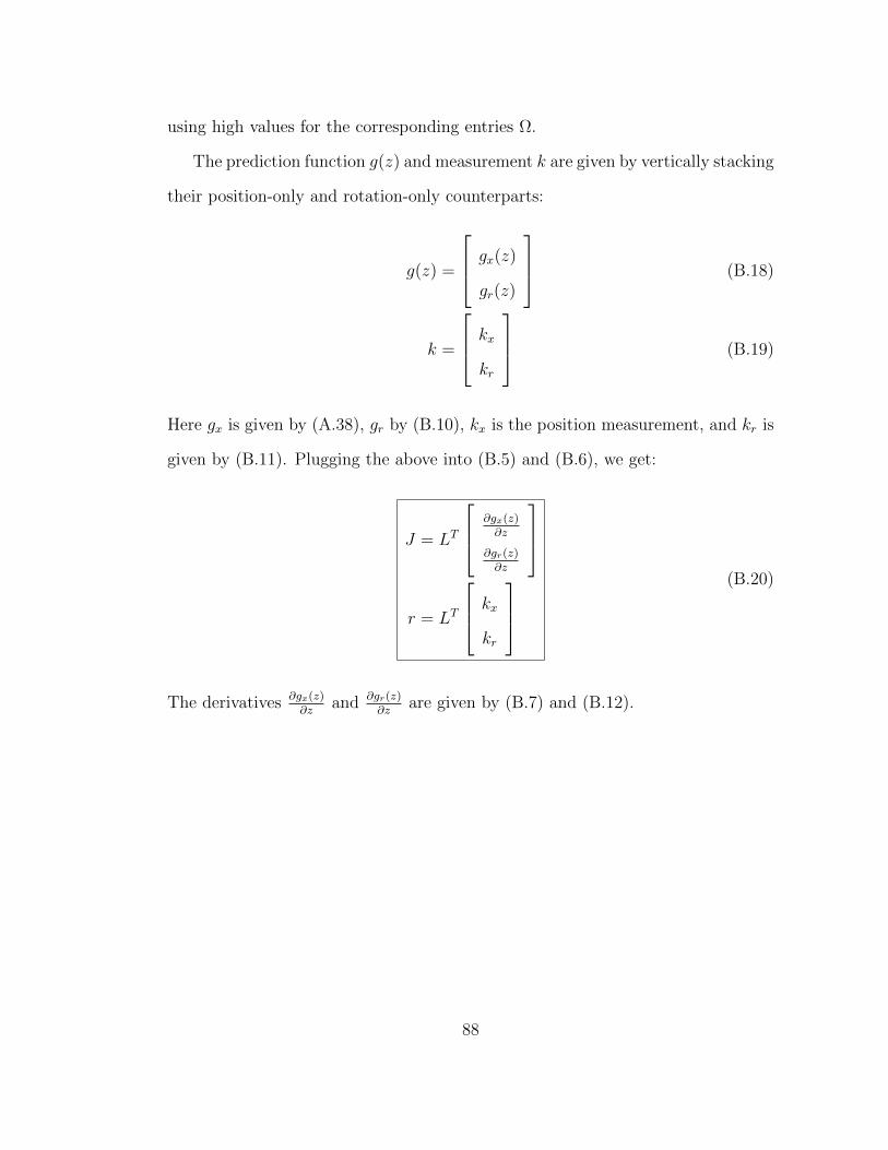
using high values for the corresponding entries Ω.

The prediction function g(z) and measurement k are given by vertically stacking

their position-only and rotation-only counterparts:

g(z) =

gx(z)

gr(z)

(B.18)

k =

kx

kr

(B.19)

Here gx is given by (A.38), gr by (B.10), kx is the position measurement, and kr is

given by (B.11). Plugging the above into (B.5) and (B.6), we get:

J = LT

∂gx(z)∂z

∂gr(z)∂z

r = LT

kx

kr

(B.20)

The derivatives ∂gx(z)∂z

and ∂gr(z)∂z

are given by (B.7) and (B.12).

88

Bibliography

[1] Motilal Agrawal and Kurt Konolige, Rough terrain visual odometry, Proceed-

ings of the International Conference on Advanced Robotics (ICAR) (2007).

xii, xvii, 6, 10, 15, 19, 20, 21, 23

[2] P Amestoy, H.S. Dollar, J.K. Reid, and J.A. Scott, An approximate minimum

degree algorithm for matrices with dense rows, Tech. report, ENSEEIHT, 2008.

47

[3] Evan Andersen and Clark Taylor, Improving mav pose estimation using visual

information, Proc. Intl. Conf. on Intelligent Robots and Systems (IROS),

IEEE, 2007, pp. 3745–3750. 8

[4] C. Bibby and I. Reid, Simultaneous localisation and mapping in dynamic envi-

ronments (slamide) with reversible data association, Proceedings of Robotics:

Science and Systems (Atlanta, GA, USA), June 2007. 6, 30

[5] Leon Bottou, Stochastic learning, Advanced Lectures on Machine Learning

(Olivier Bousquet and Ulrike von Luxburg, eds.), Lecture Notes in Artificial

Intelligence, LNAI 3176, Springer Verlag, Berlin, 2004, pp. 146–168. 28, 37

89

[6] Alison Brown and Dan Sullivan, Inertial navigation electro-optical aiding dur-

ing gps dropouts, Proceedings of the Joint Navigation Conference, 2002. 8

[7] Tim Davis, Direct methods for sparse linear systems, SIAM, 2006. 47

[8] Timothy A. Davis, Algorithm 915, SuiteSparseQR: Multifrontal multithreaded

rank-revealing sparse QR factorization, ACM Transactions on Mathematical

Software 38 (2011), no. 1. 58

[9] Andrew J. Davison, Ian D. Reid, Nicholas D. Molton, and Olivier Stasse,

Monoslam: Real-time single camera slam, IEEE Trans. Pattern Anal. Mach.

Intell. 29 (2007), no. 6, 1052–1067. 28

[10] F. Dellaert, J. Carlson, V. Ila, K. Ni, and C. E Thorpe, Subgraph-

preconditioned conjugate gradients for large scale SLAM, IROS, 2010. 30

[11] F. Dellaert and M. Kaess, Square Root SAM: Simultaneous localization and

mapping via square root information smoothing, Intl. J. of Robotics Research

(IJRR) 25 (2006), no. 12, 1181–1204. 36, 47

[12] Martin A. Fischler and Robert C. Bolles, Random sample consensus: a

paradigm for model fitting with applications to image analysis and automated

cartography, Commun. ACM 24 (1981), no. 6, 381–395. 10

[13] Garmin International, Inc., Gps16/17 series technical specifications, 2005. 9

[14] Alan George, Nested dissection of a regular finite element mesh, SIAM J. on

Numerical Analysis 10 (1972), 345–363. 43

90

[15] M. K. Grimes, D. Anguelov, and Y. LeCun, Hybrid hessians for flexible opti-

mization of pose graphs, Proc. Intl. Conf. on Intelligent Robots and Systems

(IROS), 2010. xiv, 60

[16] G. Grisetti, R. Kummerle, C. Stachniss, U. Frese, and C. Hertzberg, Hi-

erarchical optimization on manifolds for online 2d and 3d mapping, ICRA

(Anchorage, AK, USA), May 2010. 30, 53

[17] G. Grisetti, C. Stachniss, S. Grzonka, and Burgard, A tree parameterization

for efficiently computing maximum likelihood maps using gradient descent,

Proc. of Robotics: Science and Systems (RSS) (Atlanta, GA, USA), 2007.

xiii, xiv, 28, 33, 37, 39, 46, 60

[18] Raia Hadsell, Pierre Sermanet, Marco Scoffier, Ayse Erkan, Koray Kavack-

uoglu, Urs Muller, and Yann LeCun, Learning long-range vision for au-

tonomous off-road driving, J. of Field Robotics (JFR) (2009). 19

[19] Chris Harris and Mike Stephens, A combined corner and edge detector,, Pro-

ceedings of the 4th Alvey Vision Conference, 1988, pp. 147–151. 10

[20] Pinar Heggernes and Pontus Matstoms, Finding good column orderings for

sparse qr factorization, In Second SIAM Conference on Sparse Matrices, 1996.

47

[21] Christoph Hertzberg, A framework for sparse, non-linear least squares prob-

lems on manifolds, Master’s thesis, University of Bremen, 2008. 53

[22] T.M. Heskes and B. Kappen, On-line learning processes in artificial neural

networks, Mathematical Approaches to Neural Networks 51 (1993), 199–233.

37

91

[23] Bernard Hofmann-Wellenhof, Herbert Lichtenegger, and James Collins, Global

positioning system: Theory and practice, 5th ed., Springer-Verlag, 2001. 9

[24] A. Howard, Real-time stereo visual odometry for autonomous ground vehicles,

IEEE Int. Conf. on Intelligent Robots and Systems, 2008. 10

[25] Albert Huang, Abraham Bachrach, Peter Henry, Michael Krainin, Daniel Mat-

urana, Dieter Fox, and Nicholas Roy, Visual odometry and mapping for au-

tonomous flight using an rgb-d camera, Intl. Symp. of Robotics Research, 2011.

10

[26] M. Kaess, G. Grisetti, and K. Ni, Automated slam evaluation work-

shop for 2011 RSS, http://slameval.willowgarage.com/workshop/talks/

2011-RSS-SLAM-Evaluation.pdf, July 2011. 54

[27] M. Kaess, V. Ila, R. Roberts, and F. Dellaert, The Bayes tree: An algorithmic

foundation for probabilistic robot mapping, Intl. Workshop on the Algorithmic

Foundations of Robotics, WAFR (Singapore), Dec 2010. 29, 47, 48

[28] M. Kaess, K. Ni, and F. Dellaert, Flow separation for fast and robust stereo

odometry, IEEE Intl. Conf. on Robotics and Automation, ICRA (Kobe,

Japan), May 2009. 10, 21

[29] Georg Klein and David Murray, Improving the agility of keyframe-based

SLAM, Proc. 10th European Conference on Computer Vision (ECCV’08)

(Marseille), October 2008, pp. 802–815. 16

[30] Laurent Kneip, Margarita Chli, and Roland Siegwart, Robust real-time visual

odometry with a single camera and an imu, British Machine Vision Confer-

ence, 2011. 8

92

[31] K. Konolige, G. Grisetti, R. Kummerle, W. Burgard, B. Limketkai, and

R. Vincent, Sparse pose adjustment for 2d mapping, IROS (Taipei, Taiwan),

10/2010 2010. 47

[32] Y. LeCun, L. Bottou, G. Orr, and K. Muller, Efficient backprop, Neural Net-

works: Tricks of the trade (G. Orr and Muller K., eds.), Springer, 1998. 28,

37, 38

[33] Mark Maimone, Yang Cheng, and Larry Matthies, Two years of visual odom-

etry on the mars exploration rovers: Field reports, Journal of Field Robotics

24 (2007), no. 3, 169–186. 1, 8, 10

[34] Hans Moravec, Obstacle avoidance and navigation in the real world by a seeing

robot rover, Ph.D. thesis, Stanford University, 1980. 10

[35] David Nister, Oleg Naroditsky, and James Bergen, Visual odometry, Proc.

of Conf. on Computer Vision and Pattern Recognition (CVPR) 01 (2004),

652–659. 6, 10

[36] Lauro Ojeda, Daniel Cruz, Giulio Reina, and Johann Borenstein, Current-

based slippage detection and odometry correction for mobile robots and plane-

tary rovers, IEEE Trans. on Robotics, (TRO) 22 (2006), no. 2. 8

[37] Edwin Olson, Robust and efficient robotic mapping, Ph.D. thesis, MIT, Cam-

bridge, MA, USA, June 2008. xiv, 28, 59

[38] Edwin Olson, John Leonard, and Seth Teller, Fast iterative optimization of

pose graphs with poor initial estimates, Intl. Conf. on Robotics and Automa-

tion (ICRA), 2006, pp. 2262–2269. 28, 39, 56

93

[39] G. B. Orr, Dynamics and algorithms for stochastic learning, Ph.D. thesis,

Oregon Graduate Institute, 1995. 37

[40] E. Rosten and T. Drummond, Machine learning for high-speed corner detec-

tion, European Conf. on Computer Vision (ECCV), 2006. 10

[41] Hugh Durrant-Whyte Salah Sukkarieh, Eduardo Nebot, A high integrity

imu/gps navigation loop for autonomous land vehicle applications, IEEE

Trans. on Robotics, (TRO), vol. 15, June 1999. 9

[42] Davide Scaramuzza, Andrea Censi, and Kostas Danilidis, Exploiting motion

priors in visual odometry for vehicle-mounted cameras with non-holonomic

constraints, Proc. Intl. Conf. on Intelligent Robots and Systems (IROS), 2011.

10

[43] H. Schafer, P. Hahnfeld, and K. Berns, Real-time visual self-localisation in

dynamic environments, Autonome Mobile Systeme, 2007. 8

[44] Pierre Sermanet, Raia Hadsell, Marco Scoffier, Matt Grimes, Jan Ben, Ayse

Erkan, Chris Crudele, Urs Muller, and Yann LeCun, A multi-range architec-

ture for collision-free off-road robot navigation, J. of Field Robotics (JFR)

(2009). 19

[45] G. Sibley, C. Mei, I. Reid, and P. Newman, Adaptive relative bundle adjust-

ment, Proc. of Robotics: Science and Systems (RSS) (Seattle, USA), June

2009. 30, 51, 52

[46] Randall C. Smith and Peter Cheeseman, On the representation and estimation

of spatial uncertainty, Intl. J. of Robotics Research (IJRR) 5 (1986), no. 4,

56–68. 28

94

[47] S. Thrun, Y. Liu, D. Koller, A.Y. Ng, Z. Ghahramani, and H. Durrant-Whyte,

Simultaneous localization and mapping with sparse extended information fil-

ters, Intl. J. of Robotics Research (IJRR) (2004). 28

[48] Sebastian Thrun, Exploring artificial intelligence in the new millennium,

ch. Robotic mapping: a survey, pp. 1–35, Morgan Kaufmann Publishers Inc.,

San Francisco, CA, USA, 2003. 6

[49] Michael Veth and John Raquet, Two-dimensional stochastic projections for

tight integration of optical and inertial sensors for navigation, National Tech-

nical Meeting Proceedings of the Institute of Navigation, 2006, pp. 587–596.

8

[50] Matthew R. Walter, Ryan M. Eustice, and John J. Leonard, Exactly sparse ex-

tended information filters for feature-based slam, Intl. J. of Robotics Research

(IJRR) 26 (2007), no. 4, 335–359. 28

[51] Chris C. Ward and Karl Iagnemma, Classification-based wheel slip detection

and detector fusion for outdoor mobile robots, Intl. Conf. on Robotics and

Automation (ICRA), IEEE, 2007, pp. 2730–2735. 9

[52] , Model-based wheel slip detection for outdoor mobile robots,

Intl. Conf. on Robotics and Automation (ICRA), IEEE, 2007, pp. 2724–2729.

9, 16

[53] Mark D. Wheeler and Katsushi Ikeuchi, Iterative estimation of rotation and

translation using the quaternion, Tech. Report CMU-CS-95-215, Carnegie

Mellon University, December 1995. 75

95