Journal of Modern Applied StatisticalMethods

Volume 13 | Issue 2 Article 31

11-2014

Fitting Stereotype Logistic Regression Models forOrdinal Response Variables in EducationalResearch (Stata)Xing LiuEastern Connecticut State University, dliuxing@yahoo.com

Follow this and additional works at: http://digitalcommons.wayne.edu/jmasmPart of the Applied Statistics Commons, Social and Behavioral Sciences Commons, and the

Statistical Theory Commons

This Statistical Software Applications and Review is brought to you for free and open access by the Open Access Journals atDigitalCommons@WayneState. It has been accepted for inclusion in Journal of Modern Applied Statistical Methods by an authorized administrator ofDigitalCommons@WayneState.

Recommended CitationLiu, Xing (2014) "Fitting Stereotype Logistic Regression Models for Ordinal Response Variables in Educational Research (Stata),"Journal of Modern Applied Statistical Methods: Vol. 13: Iss. 2, Article 31.Available at: http://digitalcommons.wayne.edu/jmasm/vol13/iss2/31

Journal of Modern Applied Statistical Methods

November 2014, Vol. 13, No. 2, 528-545.

Copyright © 2014 JMASM, Inc.

ISSN 1538 − 9472

Dr. Liu is an Associate Professor in the Department of Education. Email him at liux@easternct.edu.

528

Statistical Software Applications and Review: Fitting Stereotype Logistic Regression Models for Ordinal Response Variables in Educational Research (Stata)

Xing Liu Eastern Connecticut State University

Willimantic, CT

The stereotype logistic (SL) model is an alternative to the proportional odds (PO) model for ordinal response variables when the proportional odds assumption is violated. This model seems to be underutilized. One major reason is the constraint of current statistical software packages. Statistical Package for the Social Sciences (SPSS) cannot perform the SL regression analysis, and SAS does not have the procedure developed to directly estimate the model. The purpose of this article was to illustrate the stereotype logistic (SL) regression model, and apply it to estimate mathematics proficiency level of high school

students using Stata. In addition, it compared the results of fitting the PO model and the SL model. Data from the High School Longitudinal Study of 2009 (HSLS: 2009) (Ingels, et al., 2011) were used for the ordinal regression analyses. Keywords: Stereotype logistic models, Proportional Odds models, ordinal logistic regression, ordinal response variables, Stata

Introduction

Three types of logistic regression models are well-known for analyzing the ordinal

response variable, including the proportional odds (PO) model, the continuation

ratio (CR) model, and the adjacent categories (AC) logistic regression model.

Among them, the PO model is the most commonly used (Agresti, 2002, 2007, 2010;

Armstrong & Sloan, 1989; Clogg, & Shihadeh, 1994; Hilbe, 2009; Liu, 2009; Long,

1997, Long & Freese, 2006; McCullagh, 1980; McCullagh & Nelder, 1989;

O’Connell, 2000, 2006; O’Connell & Liu, 2011; Powers & Xie, 2000).

XING LIU

529

The PO model assumes that the underlying binary models, which dichotomize

the ordinal response variable, have the same coefficients. In other words, the logit

coefficients for each predictor are the same across the ordinal categories. This is

called the parallel lines or the proportional odds (PO) assumption. However, the

PO assumption is often violated. To deal with this issue, the partial proportional

odds (PPO) model or the generalized ordinal logit model (Fu, 1998; Liu & Koirala,

2012; Peterson & Harrell, 1990; Williams, 2006) can be used. An alternative option

is the stereotype logistic (SL) model, which was first developed by Anderson

(1984), and later introduced by Greenland (1994), and Long and Freese (2006). The

SL model is an extension of both the multinomial logistic regression model and the

PO model. First, the SL model is like the multinomial logistic model since they

both estimate the odds of being at a particular category compared to the baseline

category. Second, similar to the PO model, the SL model estimates the ordinal

response variable rather than the nominal outcome variable, given a set of

predictors. However, the SL model does not assume the PO assumption, and allows

the effect of each predictor to vary across the ordinal categories.

Although the theory of the SL model has existed, this model seemed to be

underutilized: the illustration and application of this model were rare. One major

reason is the restriction of current statistical software packages. SPSS cannot

perform the SL regression analysis, and SAS does not have the procedure

developed to directly estimate the SL model. Both Anderson (1984) and Greenland

(1994) used GAUSS to fit the SL model but no programming information was

provided. Agresti (2010) recently discussed this model using the results of the two

examples directly from Anderson (1984). Kuss (2006) pioneered the use the PROC

NLMIXED procedure in SAS to estimate the SL model although it does not deal

with any random effects in the example. Researchers need to specify the starting

values, and the model equations, and the probabilities in the syntax, which is

complicated and error-prone for novice SAS users. Therefore, it is critical to help

researchers to familiarize with this model and clarify the confusion so that they are

able to apply it correctly in practice.

To fill this gap, the purpose of this study was to illustrate the use of the

stereotype logistic (SL) regression with Stata, and compare the results of fitting the

PO model and the SL model. This article is an extension of previous research on

various ordinal logistic regression models (Liu, 2009; Liu, O’Connell & Koirala,

2011; Liu & Koirala, 2012; O’Connell & Liu, 2010). For demonstration purposes,

the empirical data from the High School Longitudinal Study of 2009 (HSLS: 2009)

(Ingels, et al., 2011) were used to conduct the ordinal regression analyses.

STEREOTYPE LOGISTIC REGRESSION MODELS

530

Theoretical Framework

The Proportional Odds Model

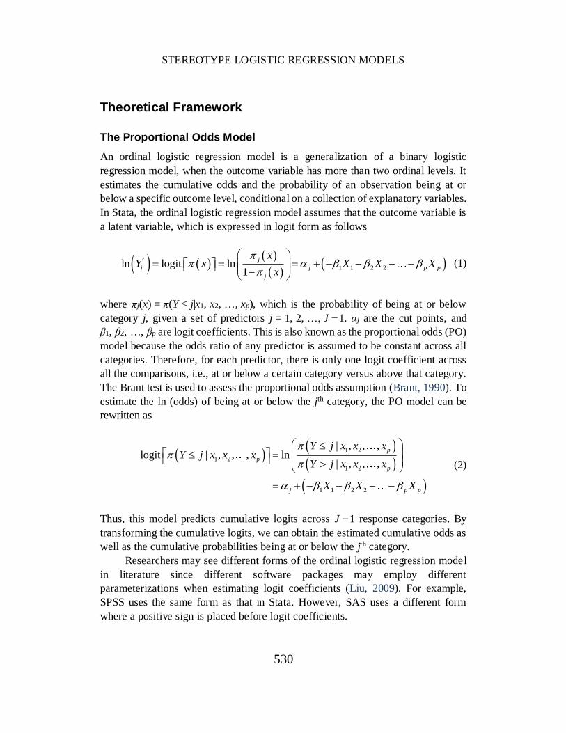
An ordinal logistic regression model is a generalization of a binary logistic

regression model, when the outcome variable has more than two ordinal levels. It

estimates the cumulative odds and the probability of an observation being at or

below a specific outcome level, conditional on a collection of explanatory variables.

In Stata, the ordinal logistic regression model assumes that the outcome variable is

a latent variable, which is expressed in logit form as follows

1 1 2 2ln logit ln

1

j

i j p p

j

xY x X X X

x

(1)

where πj(x) = π(Y ≤ j|x1, x2, …, xp), which is the probability of being at or below

category j, given a set of predictors j = 1, 2, …, J −1. αj are the cut points, and

β1, β2, …, βp are logit coefficients. This is also known as the proportional odds (PO)

model because the odds ratio of any predictor is assumed to be constant across all

categories. Therefore, for each predictor, there is only one logit coefficient across

all the comparisons, i.e., at or below a certain category versus above that category.

The Brant test is used to assess the proportional odds assumption (Brant, 1990). To

estimate the ln (odds) of being at or below the jth category, the PO model can be

rewritten as

1 2

1 2

1 2

1 1 2 2

| , , ,logit | , , , ln

| , , ,

p

p

p

j p p

Y j x x xY j x x x

Y j x x x

X X X

(2)

Thus, this model predicts cumulative logits across J −1 response categories. By

transforming the cumulative logits, we can obtain the estimated cumulative odds as

well as the cumulative probabilities being at or below the jth category.

Researchers may see different forms of the ordinal logistic regression model

in literature since different software packages may employ different

parameterizations when estimating logit coefficients (Liu, 2009). For example,

SPSS uses the same form as that in Stata. However, SAS uses a different form

where a positive sign is placed before logit coefficients.

XING LIU

531

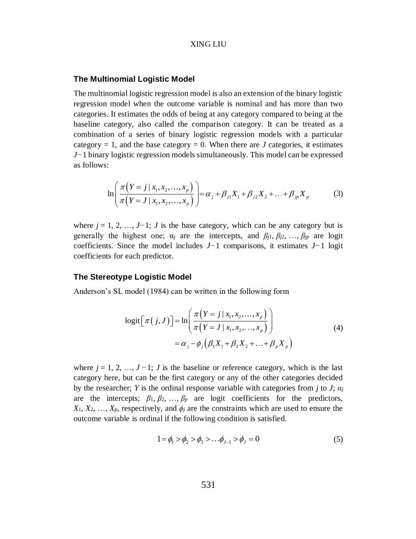
The Multinomial Logistic Model

The multinomial logistic regression model is also an extension of the binary logistic

regression model when the outcome variable is nominal and has more than two

categories. It estimates the odds of being at any category compared to being at the

baseline category, also called the comparison category. It can be treated as a

combination of a series of binary logistic regression models with a particular

category = 1, and the base category = 0. When there are J categories, it estimates

J−1 binary logistic regression models simultaneously. This model can be expressed

as follows:

1 2

1 1 2 2

1 2

| , , ,ln

| , , ,

p

j j j jp p

p

Y j x x xX X X

Y J x x x

(3)

where j = 1, 2, …, J−1; J is the base category, which can be any category but is

generally the highest one; αj are the intercepts, and βj1, βj2, …, βjp are logit

coefficients. Since the model includes J−1 comparisons, it estimates J−1 logit

coefficients for each predictor.

The Stereotype Logistic Model

Anderson’s SL model (1984) can be written in the following form

1 2

1 2

1 1 2 2

| , , ,logit , ln

| , , ,

p

p

j j p p

Y j x x xj J

Y J x x x

X X X

(4)

where j = 1, 2, …, J −1; J is the baseline or reference category, which is the last

category here, but can be the first category or any of the other categories decided

by the researcher; Y is the ordinal response variable with categories from j to J; αj

are the intercepts; β1, β2, …, βp are logit coefficients for the predictors,

X1, X2, …, Xp, respectively, and ϕj are the constraints which are used to ensure the

outcome variable is ordinal if the following condition is satisfied.

1 2 3 11 0J J (5)

STEREOTYPE LOGISTIC REGRESSION MODELS

532

The first constraint, ϕ1 is set to be 1, and the last one, ϕJ is equal to 0 so that

the estimated SL model can be identified. If any two pairs of the constraints are the

same, then these two categories are indistinguishable, thus can be collapsed into

one. For example, if ϕ3 = ϕ4, these two categories (categories 3 and 4) can be

grouped together. The ordinality of the constraints can be tested in the model so

that researchers can decide whether any categories need to be merged or re-ordered.

To calculate the odds of being in a category j versus a category m, we just

need to take the exponential of [(αj − αm) − (ϕj − ϕm)β]. When the category m

becomes the baseline category J, we just need to substitute it into the equation.

Since ϕJ = 0, we get [(αj − 0) − (ϕj − 0)β] = αj − ϕjβ. By exponentiating (−ϕjβ), we

get the odds of being in a category j versus the baseline category J for a unit change

in a predictor.

The equation (4) is the forms for Anderson’s one-dimension SL model, which

was generally referred to as the SL model in literature. Anderson (1984) also argued

that an ordinal response variable could be more than one dimension, and therefore

proposed the multidimensional SL model. If the ordinal outcome variable has J

categories, the maximum dimensions would be J−1. The multidimensional SL

model with J−1 dimensions is actually equal to the multinomial logistic regression

model. In this article, we only focus on the one-dimension SL model for the

simplicity of model building and interpretation.

Lunt (2001) considered the SL model as the constrained multinomial logistic

model, and developed the Stata soreg program before the official Stata slogit

program was implemented. Compared with the multinomial logistic regression

model in the equation (3), the left side of the logit link function for the SL model

in the equation (4) looks the same, since both the SL model and the multinomial

model estimates the odds of being in a particular category versus the baseline

category. Examining the systematic component (linear predictors) in both models,

it is obvious that the logit coefficients, βj in the multinomial logistic model

corresponds to (−ϕj(β)) in the SL model. When there are J categories of the outcome

variable and p predictors, we need to estimate (J−1) + (J−1)×p parameters in the

multinomial logistic model, which also equals (J−1)×(1+p). In the SL model, we

estimate [(J−1) + (J−2) + p] = (2J − 3+p) parameters since ϕ1 and ϕJ are

constrained to be 1 and 0, respectively. Therefore, less parameters are estimated in

the SL model than in the multinomial logistic model, and the former model is more

parsimonious.

XING LIU

533

Methodology

Sample

Similar to the previous Education Longitudinal Study of 2002 (ELS: 2002), the

HSLS: 2009 study, conducted by the NCES, was the latest series of longitudinal

study in secondary schools. This study surveyed high school students, parents,

teachers, school counselors and administrators, and assessed 9th graders’ algebraic

skills and reasoning. It was designed to keep track of high school students from

grade nine to postsecondary school education and their choice of future careers. In

the 2009 base year data, 21,444 high school students, from a national sample of 944

schools, participated in the study. Students were asked to provide information

regarding basic demographics, school and home experience, such as math and

science activities, coursework, and time spent on different activities, mathematics

and science attitude, mathematics and science self-efficacy, their feelings about

math and science teacher, and future educational and life plans after secondary

schools. The ordinal outcome variable is students’ mathematics proficiency, and

the predictors are students’ math identity (MTHID), mathematics self-efficacy

(MTHEFF), school belonging (SCHBEL), and school engagement (SCHENG).

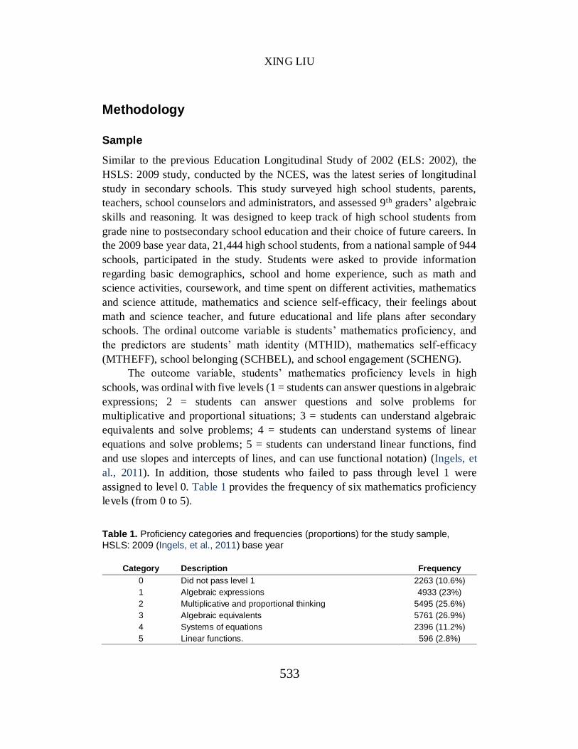
The outcome variable, students’ mathematics proficiency levels in high

schools, was ordinal with five levels (1 = students can answer questions in algebraic

expressions; 2 = students can answer questions and solve problems for

multiplicative and proportional situations; 3 = students can understand algebraic

equivalents and solve problems; 4 = students can understand systems of linear

equations and solve problems; 5 = students can understand linear functions, find

and use slopes and intercepts of lines, and can use functional notation) (Ingels, et

al., 2011). In addition, those students who failed to pass through level 1 were

assigned to level 0. Table 1 provides the frequency of six mathematics proficiency

levels (from 0 to 5). Table 1. Proficiency categories and frequencies (proportions) for the study sample,

HSLS: 2009 (Ingels, et al., 2011) base year

Category Description Frequency

0 Did not pass level 1 2263 (10.6%)

1 Algebraic expressions 4933 (23%)

2 Multiplicative and proportional thinking 5495 (25.6%)

3 Algebraic equivalents 5761 (26.9%)

4 Systems of equations 2396 (11.2%)

5 Linear functions. 596 (2.8%)

STEREOTYPE LOGISTIC REGRESSION MODELS

534

Data Analysis

First, the PO model was used for the preliminary analysis with the Stata ologit

command, and the proportional odds assumption was examined using the Brant test.

Then the SL model with a single explanatory variable was fitted using the Stata

slogit command. Finally the full-model with all four explanatory variables was

fitted. Model fit statistics for both the PO model and the SL model were provided

by the Stata SPost package (Long & Freese, 2006). The results for both models

were interpreted and compared. Following the suggestion by Hardin and Hilbe

(2007) and Hilbe (2009), Stata AIC and BIC statistics were used for the comparison

of model fit.

Results

The Proportional Odds Model with Four Explanatory Variables

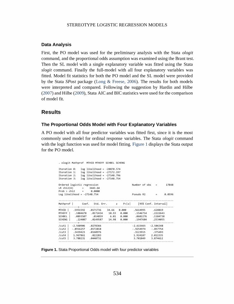
A PO model with all four predictor variables was fitted first, since it is the most

commonly used model for ordinal response variables. The Stata ologit command

with the logit function was used for model fitting. Figure 1 displays the Stata output

for the PO model.

. ologit Mathprof MTHID MTHEFF SCHBEL SCHENG Iteration 0: log likelihood = -28870.574 Iteration 1: log likelihood = -27172.197 Iteration 2: log likelihood = -27148.796 Iteration 3: log likelihood = -27148.754 Ordered logistic regression Number of obs = 17848 LR chi2(4) = 3443.64 Prob > chi2 = 0.0000 Log likelihood = -27148.754 Pseudo R2 = 0.0596 ------------------------------------------------------------------------------ Mathprof | Coef. Std. Err. z P>|z| [95% Conf. Interval] -------------+---------------------------------------------------------------- MTHID | .5951592 .0171736 34.66 0.000 .5614995 .628819 MTHEFF | .1884678 .0172434 10.93 0.000 .1546714 .2222643 SCHBEL | .0893507 .014859 6.01 0.000 .0602276 .1184738 SCHENG | .224087 .0149587 14.98 0.000 .1947684 .2534055 -------------+---------------------------------------------------------------- /cut1 | -2.560906 .0278366 -2.615465 -2.506348 /cut2 | -.8916257 .0172818 -.9254974 -.857754 /cut3 | .3439423 .0160976 .3123915 .375493 /cut4 | 1.967861 .022283 1.924187 2.011535 /cut5 | 3.788231 .0440731 3.701849 3.874612 ------------------------------------------------------------------------------

Figure 1. Stata Proportional Odds model with four predictor variables

XING LIU

535

The log likelihood ratio Chi-Square test, LR χ2(4) = 3443.64, p < .001,

indicating that the full model with four predictor provided a better fit than the null

model with no independent variables.

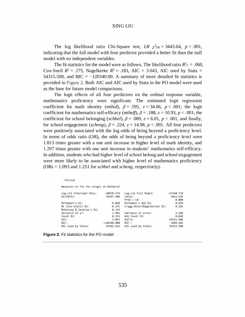
The fit statistics for the model were as follows. The likelihood ratio R2L = .060,

Cox-Snell R2 = .175, Nagelkerke R2 = .183, AIC = 3.043, AIC used by Stata =

54315.508, and BIC = −120340.00. A summary of more detailed fit statistics is

provided in Figure 2. Both AIC and AIC used by Stata in the PO model were used

as the base for future model comparisons.

The logit effects of all four predictors on the ordinal response variable,

mathematics proficiency were significant. The estimated logit regression

coefficient for math identity (mthid), β = .595, z = 34.66, p < .001; the logit

coefficient for mathematics self-efficacy (mtheff), β = .188, z = 10.93, p < .001; the

coefficient for school belonging (schbel), β = .089, z = 6.01, p < .001, and finally,

for school engagement (scheng), β = .224, z = 14.98, p < .001. All four predictors

were positively associated with the log odds of being beyond a proficiency level.

In terms of odds ratio (OR), the odds of being beyond a proficiency level were

1.813 times greater with a one unit increase in higher level of math identity, and

1.207 times greater with one unit increase in students’ mathematics self-efficacy.

In addition, students who had higher level of school belong and school engagement

were more likely to be associated with higher level of mathematics proficiency

(ORs = 1.093 and 1.251 for schbel and scheng, respectively).

. fitstat Measures of Fit for ologit of Mathprof Log-Lik Intercept Only: -28870.574 Log-Lik Full Model: -27148.754 D(17839): 54297.508 LR(4): 3443.639 Prob > LR: 0.000 McFadden's R2: 0.060 McFadden's Adj R2: 0.059 ML (Cox-Snell) R2: 0.175 Cragg-Uhler(Nagelkerke) R2: 0.183 McKelvey & Zavoina's R2: 0.174 Variance of y*: 3.983 Variance of error: 3.290 Count R2: 0.331 Adj Count R2: 0.068 AIC: 3.043 AIC*n: 54315.508 BIC: -120340.000 BIC': -3404.481 BIC used by Stata: 54385.615 AIC used by Stata: 54315.508

Figure 2. Fit statistics for the PO model

STEREOTYPE LOGISTIC REGRESSION MODELS

536

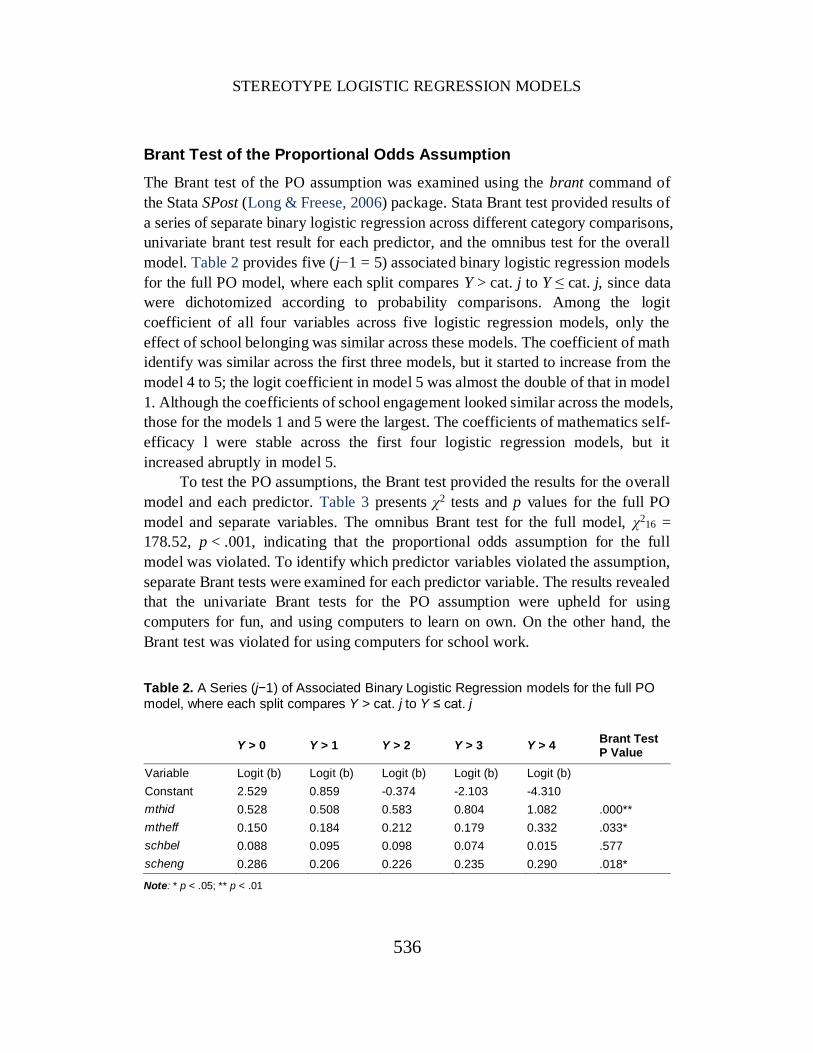
Brant Test of the Proportional Odds Assumption

The Brant test of the PO assumption was examined using the brant command of

the Stata SPost (Long & Freese, 2006) package. Stata Brant test provided results of

a series of separate binary logistic regression across different category comparisons,

univariate brant test result for each predictor, and the omnibus test for the overall

model. Table 2 provides five (j−1 = 5) associated binary logistic regression models

for the full PO model, where each split compares Y > cat. j to Y ≤ cat. j, since data

were dichotomized according to probability comparisons. Among the logit

coefficient of all four variables across five logistic regression models, only the

effect of school belonging was similar across these models. The coefficient of math

identify was similar across the first three models, but it started to increase from the

model 4 to 5; the logit coefficient in model 5 was almost the double of that in model

1. Although the coefficients of school engagement looked similar across the models,

those for the models 1 and 5 were the largest. The coefficients of mathematics self-

efficacy l were stable across the first four logistic regression models, but it

increased abruptly in model 5.

To test the PO assumptions, the Brant test provided the results for the overall

model and each predictor. Table 3 presents χ2 tests and p values for the full PO

model and separate variables. The omnibus Brant test for the full model, χ216 =

178.52, p < .001, indicating that the proportional odds assumption for the full

model was violated. To identify which predictor variables violated the assumption,

separate Brant tests were examined for each predictor variable. The results revealed

that the univariate Brant tests for the PO assumption were upheld for using

computers for fun, and using computers to learn on own. On the other hand, the

Brant test was violated for using computers for school work. Table 2. A Series (j−1) of Associated Binary Logistic Regression models for the full PO

model, where each split compares Y > cat. j to Y ≤ cat. j

Y > 0 Y > 1 Y > 2 Y > 3 Y > 4 Brant Test P Value

Variable Logit (b) Logit (b) Logit (b) Logit (b) Logit (b)

Constant 2.529 0.859 -0.374 -2.103 -4.310

mthid 0.528 0.508 0.583 0.804 1.082 .000**

mtheff 0.150 0.184 0.212 0.179 0.332 .033*

schbel 0.088 0.095 0.098 0.074 0.015 .577

scheng 0.286 0.206 0.226 0.235 0.290 .018*

Note: * p < .05; ** p < .01

XING LIU

537

Table 3. Brant tests of the PO assumption for each predictor and the overall model

Variable Test P Value

mthid χ24 = 101.01 .000**

mtheff χ24 = 10.48 .033*

schbel χ24 = 2.88 .577

scheng χ24 = 11.91 .018*

All (Full-model) χ216 = 178.52 .000**

Note: * p < .05; ** p < .01

The Stereotype Logistic Regression Model with a Single Explanatory

Variable

Stereotype logistic regression models were fitted since they released the PO

assumption and allowed the logit coefficients to vary across the ordinal categories.

For comparison purposes, model fitting process included both a single variable

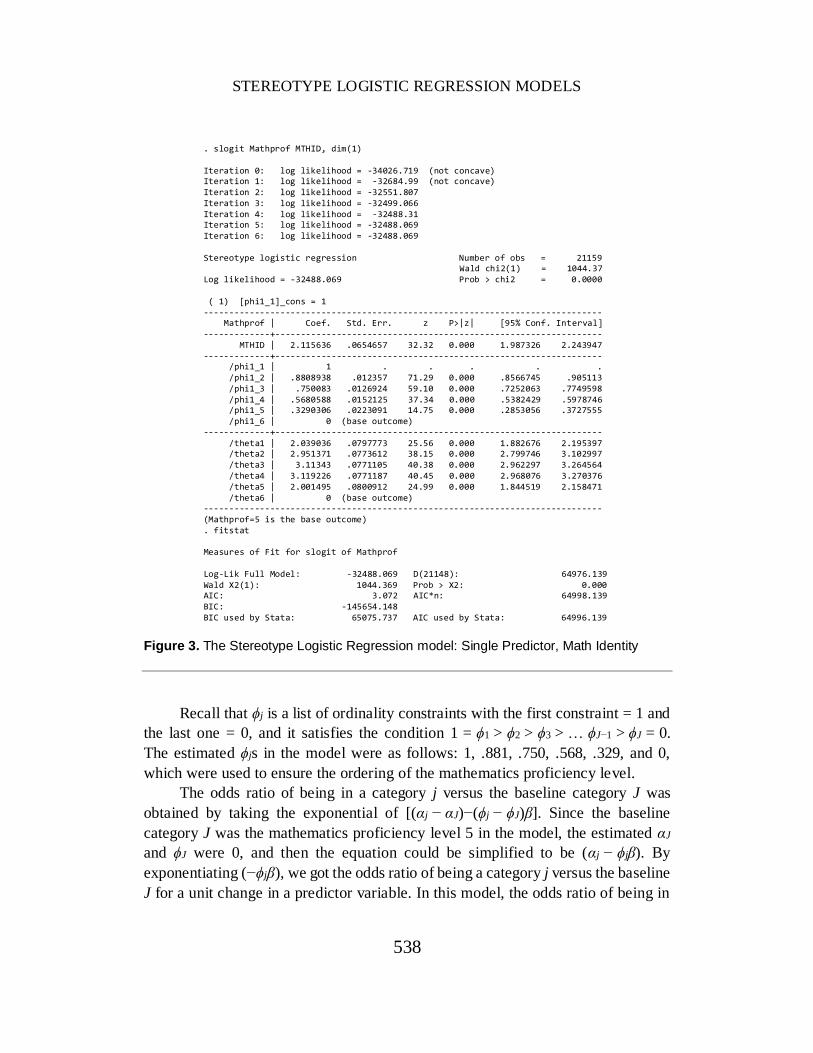
model and the full model with all four predictor variables. Figure 3 presents the

Stata output for the single predictor SL model.

The Wald Chi-Square test with 1 degree of freedom, Wald χ2(1) = 1044.37,

p < .001, indicating that the logit coefficient of the predictor, math identity was

statistically different from 0. Since no R2 statistics were calculated, only the AIC

and BIC statistics were reported. The AIC statistic was 3.072, and the AIC used by

Stata was 64996.139. BIC was −145654.148, and the corresponding BIC used by

Stat was 65075.737.

The estimated logit coefficient, β = 2.116, z = 32.32, p < .001, indicating that

students’ math identity had a significant relationship with mathematics proficiency.

The SL model estimates the logit odds of being in a category relative to the

baseline category. Substituting the value of the coefficient into the formula (4)

1

1 1

1

|ln ,

|j j

Y j xX

Y J x

we calculated

logit , | *2.116 .j jj J mathid mathid

STEREOTYPE LOGISTIC REGRESSION MODELS

538

. slogit Mathprof MTHID, dim(1) Iteration 0: log likelihood = -34026.719 (not concave) Iteration 1: log likelihood = -32684.99 (not concave) Iteration 2: log likelihood = -32551.807 Iteration 3: log likelihood = -32499.066 Iteration 4: log likelihood = -32488.31 Iteration 5: log likelihood = -32488.069 Iteration 6: log likelihood = -32488.069 Stereotype logistic regression Number of obs = 21159 Wald chi2(1) = 1044.37 Log likelihood = -32488.069 Prob > chi2 = 0.0000 ( 1) [phi1_1]_cons = 1 ------------------------------------------------------------------------------ Mathprof | Coef. Std. Err. z P>|z| [95% Conf. Interval] -------------+---------------------------------------------------------------- MTHID | 2.115636 .0654657 32.32 0.000 1.987326 2.243947 -------------+---------------------------------------------------------------- /phi1_1 | 1 . . . . . /phi1_2 | .8808938 .012357 71.29 0.000 .8566745 .905113 /phi1_3 | .750083 .0126924 59.10 0.000 .7252063 .7749598 /phi1_4 | .5680588 .0152125 37.34 0.000 .5382429 .5978746 /phi1_5 | .3290306 .0223091 14.75 0.000 .2853056 .3727555 /phi1_6 | 0 (base outcome) -------------+---------------------------------------------------------------- /theta1 | 2.039036 .0797773 25.56 0.000 1.882676 2.195397 /theta2 | 2.951371 .0773612 38.15 0.000 2.799746 3.102997 /theta3 | 3.11343 .0771105 40.38 0.000 2.962297 3.264564 /theta4 | 3.119226 .0771187 40.45 0.000 2.968076 3.270376 /theta5 | 2.001495 .0800912 24.99 0.000 1.844519 2.158471 /theta6 | 0 (base outcome) ------------------------------------------------------------------------------ (Mathprof=5 is the base outcome) . fitstat Measures of Fit for slogit of Mathprof Log-Lik Full Model: -32488.069 D(21148): 64976.139 Wald X2(1): 1044.369 Prob > X2: 0.000 AIC: 3.072 AIC*n: 64998.139 BIC: -145654.148 BIC used by Stata: 65075.737 AIC used by Stata: 64996.139

Figure 3. The Stereotype Logistic Regression model: Single Predictor, Math Identity

Recall that ϕj is a list of ordinality constraints with the first constraint = 1 and

the last one = 0, and it satisfies the condition 1 = ϕ1 > ϕ2 > ϕ3 > … ϕJ−1 > ϕJ = 0.

The estimated ϕjs in the model were as follows: 1, .881, .750, .568, .329, and 0,

which were used to ensure the ordering of the mathematics proficiency level.

The odds ratio of being in a category j versus the baseline category J was

obtained by taking the exponential of [(αj − αJ)−(ϕj − ϕJ)β]. Since the baseline

category J was the mathematics proficiency level 5 in the model, the estimated αJ

and ϕJ were 0, and then the equation could be simplified to be (αj − ϕjβ). By

exponentiating (−ϕjβ), we got the odds ratio of being a category j versus the baseline

J for a unit change in a predictor variable. In this model, the odds ratio of being in

XING LIU

539

mathematics proficiency level 0 compared to being in level 5,

OR(0,5) = e(−1*2.116) = e(−2.116) = .121. This indicated that for a unit increase in math

identity the odds of being in mathematics proficiency level 0 compared to being the

baseline category 5 decreased by a factor of .121. In other words, students were

more likely to be in the highest proficiency level 5 rather than being in level 0 when

students had higher level of math identity.

Since ϕ2 = .881, the odds ratio of being in mathematics proficiency level 1

compared to being in level 5, OR(1,5) = e(−.881*2.116) = e(−1.864) = .155. Since ϕ3, ϕ4,

and ϕ5 were .750, .568, and .329, respectively, the odds ratio of being in the other

proficiency levels compared to being in the baseline level were calculated in the

same way. OR(2,5), OR(3,5) and OR(4,5) were .205, .301, and .498 respectively.

The odds of being in the baseline category J, relative to a particular category

j, is the inverse of the odds of being in that category versus the baseline category.

To estimate the odds of being in the baseline category relative to a particular

category, we just need to change the signs before the cutpoints and the estimated

logits in the equation (6). The modified logit equation,

logit[π(J, j | mthid)] = −αj + ϕj × 2.116(mthid). By exponentiating (ϕjβ), we get the

odds ratio of being in the baseline category J versus any other category for a one

unit change in a predictor variable.

OR(5,0) = e(1*2.116) = 8.295, indicating that the odds of being in the

proficiency level 5 relative to the level 0 were 8.295 times greater with one unit

increase in math identity. The odds ratio of being in the baseline level 5 compared

to being in level 1, OR(5,1) = e(.881*2.116) = e(1.864) = 6.449. The ORs of being the

baseline category versus the other three categories were computed in the same way,

and they were 4.889, 3.326, and 2.006, respectively.

The Full Stereotype Logistic Regression Model with Four Predictor

Variables

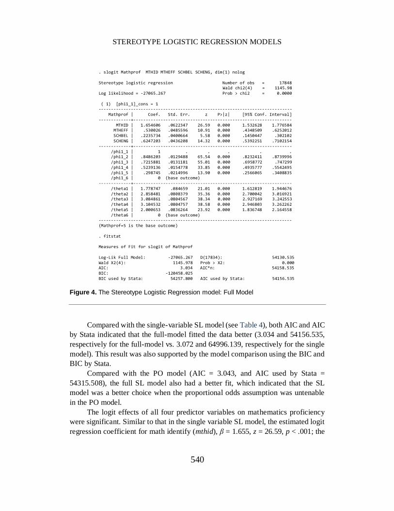
Next, the full SL model with all four predictor variables was fitted. Figure 4 and

Table 4 provide the results of the full SL model. The Wald Chi-Square test, Wald

χ2(4) = 1145.98, p < .001, indicating that the full model provides a better fit than the

null model. The AIC statistic was 3.034, and the AIC used by Stata was 54156.535.

BIC was −120458.025, and the corresponding BIC used by Stata was 54257.800.

STEREOTYPE LOGISTIC REGRESSION MODELS

540

. slogit Mathprof MTHID MTHEFF SCHBEL SCHENG, dim(1) nolog Stereotype logistic regression Number of obs = 17848 Wald chi2(4) = 1145.98 Log likelihood = -27065.267 Prob > chi2 = 0.0000 ( 1) [phi1_1]_cons = 1 ------------------------------------------------------------------------------ Mathprof | Coef. Std. Err. z P>|z| [95% Conf. Interval] -------------+---------------------------------------------------------------- MTHID | 1.654606 .0622347 26.59 0.000 1.532628 1.776584 MTHEFF | .530026 .0485596 10.91 0.000 .4348509 .6252012 SCHBEL | .2235734 .0400664 5.58 0.000 .1450447 .302102 SCHENG | .6247203 .0436208 14.32 0.000 .5392251 .7102154 -------------+---------------------------------------------------------------- /phi1_1 | 1 . . . . . /phi1_2 | .8486203 .0129488 65.54 0.000 .8232411 .8739996 /phi1_3 | .7215881 .0131181 55.01 0.000 .6958772 .747299 /phi1_4 | .5239136 .0154778 33.85 0.000 .4935777 .5542495 /phi1_5 | .298745 .0214996 13.90 0.000 .2566065 .3408835 /phi1_6 | 0 (base outcome) -------------+---------------------------------------------------------------- /theta1 | 1.778747 .084659 21.01 0.000 1.612819 1.944676 /theta2 | 2.858481 .0808379 35.36 0.000 2.700042 3.016921 /theta3 | 3.084861 .0804567 38.34 0.000 2.927169 3.242553 /theta4 | 3.104532 .0804757 38.58 0.000 2.946803 3.262262 /theta5 | 2.000653 .0836264 23.92 0.000 1.836748 2.164558 /theta6 | 0 (base outcome) ------------------------------------------------------------------------------ (Mathprof=5 is the base outcome) . fitstat Measures of Fit for slogit of Mathprof Log-Lik Full Model: -27065.267 D(17834): 54130.535 Wald X2(4): 1145.978 Prob > X2: 0.000 AIC: 3.034 AIC*n: 54158.535 BIC: -120458.025 BIC used by Stata: 54257.800 AIC used by Stata: 54156.535

Figure 4. The Stereotype Logistic Regression model: Full Model

Compared with the single-variable SL model (see Table 4), both AIC and AIC

by Stata indicated that the full-model fitted the data better (3.034 and 54156.535,

respectively for the full-model vs. 3.072 and 64996.139, respectively for the single

model). This result was also supported by the model comparison using the BIC and

BIC by Stata.

Compared with the PO model (AIC = 3.043, and AIC used by Stata =

54315.508), the full SL model also had a better fit, which indicated that the SL

model was a better choice when the proportional odds assumption was untenable

in the PO model.

The logit effects of all four predictor variables on mathematics proficiency

were significant. Similar to that in the single variable SL model, the estimated logit

regression coefficient for math identify (mthid), β = 1.655, z = 26.59, p < .001; the

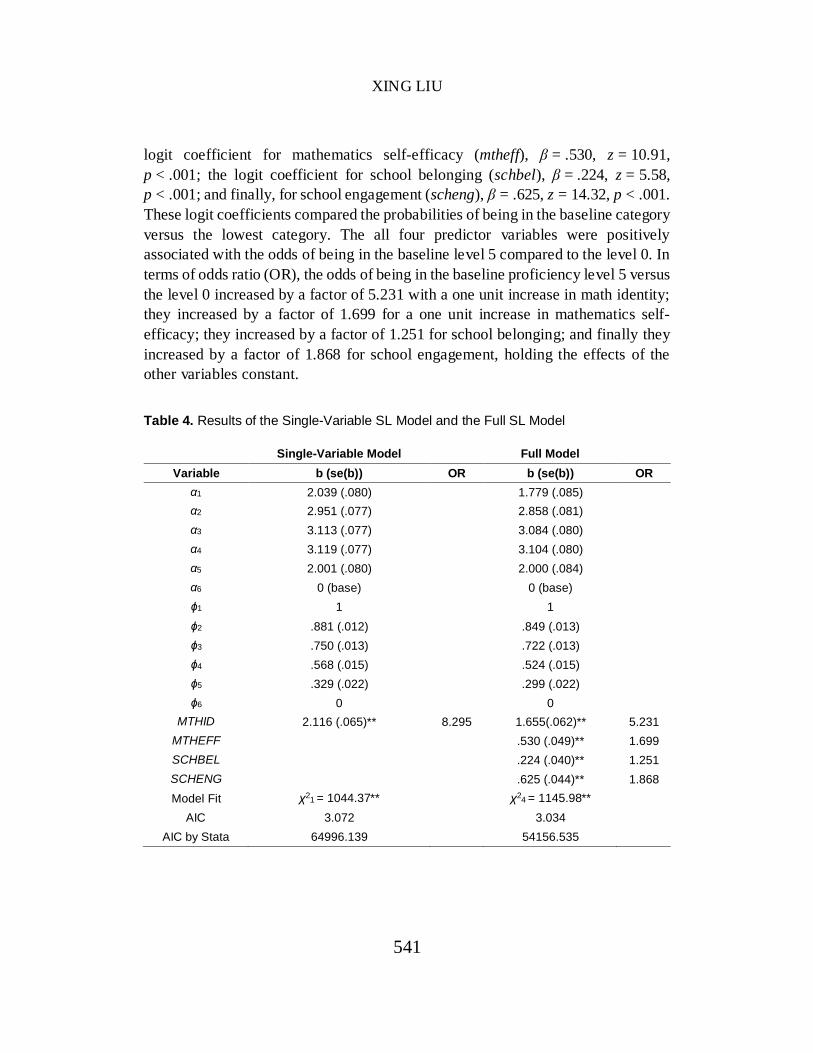
XING LIU

541

logit coefficient for mathematics self-efficacy (mtheff), β = .530, z = 10.91,

p < .001; the logit coefficient for school belonging (schbel), β = .224, z = 5.58,

p < .001; and finally, for school engagement (scheng), β = .625, z = 14.32, p < .001.

These logit coefficients compared the probabilities of being in the baseline category

versus the lowest category. The all four predictor variables were positively

associated with the odds of being in the baseline level 5 compared to the level 0. In

terms of odds ratio (OR), the odds of being in the baseline proficiency level 5 versus

the level 0 increased by a factor of 5.231 with a one unit increase in math identity;

they increased by a factor of 1.699 for a one unit increase in mathematics self-

efficacy; they increased by a factor of 1.251 for school belonging; and finally they

increased by a factor of 1.868 for school engagement, holding the effects of the

other variables constant. Table 4. Results of the Single-Variable SL Model and the Full SL Model

Single-Variable Model Full Model

Variable b (se(b)) OR b (se(b)) OR

α1 2.039 (.080) 1.779 (.085)

α2 2.951 (.077) 2.858 (.081)

α3 3.113 (.077) 3.084 (.080)

α4 3.119 (.077) 3.104 (.080)

α5 2.001 (.080) 2.000 (.084)

α6 0 (base) 0 (base)

ϕ1 1 1

ϕ2 .881 (.012) .849 (.013)

ϕ3 .750 (.013) .722 (.013)

ϕ4 .568 (.015) .524 (.015)

ϕ5 .329 (.022) .299 (.022)

ϕ6 0 0

MTHID 2.116 (.065)** 8.295 1.655(.062)** 5.231

MTHEFF .530 (.049)** 1.699

SCHBEL .224 (.040)** 1.251

SCHENG .625 (.044)** 1.868

Model Fit χ21 = 1044.37** χ2

4 = 1145.98**

AIC 3.072 3.034

AIC by Stata 64996.139 54156.535

STEREOTYPE LOGISTIC REGRESSION MODELS

542

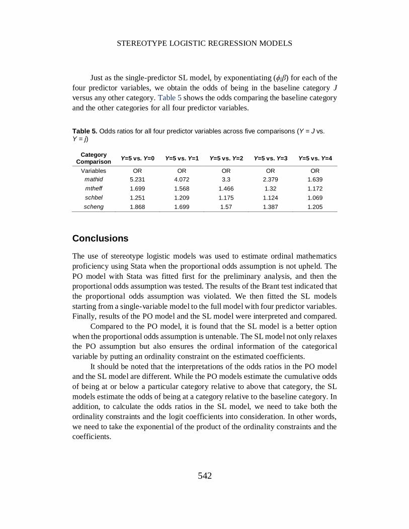
Just as the single-predictor SL model, by exponentiating (ϕjβ) for each of the

four predictor variables, we obtain the odds of being in the baseline category J

versus any other category. Table 5 shows the odds comparing the baseline category

and the other categories for all four predictor variables. Table 5. Odds ratios for all four predictor variables across five comparisons (Y = J vs. Y = j)

Category Comparison

Y=5 vs. Y=0 Y=5 vs. Y=1 Y=5 vs. Y=2 Y=5 vs. Y=3 Y=5 vs. Y=4

Variables OR OR OR OR OR

mathid 5.231 4.072 3.3 2.379 1.639

mtheff 1.699 1.568 1.466 1.32 1.172

schbel 1.251 1.209 1.175 1.124 1.069

scheng 1.868 1.699 1.57 1.387 1.205

Conclusions

The use of stereotype logistic models was used to estimate ordinal mathematics

proficiency using Stata when the proportional odds assumption is not upheld. The

PO model with Stata was fitted first for the preliminary analysis, and then the

proportional odds assumption was tested. The results of the Brant test indicated that

the proportional odds assumption was violated. We then fitted the SL models

starting from a single-variable model to the full model with four predictor variables.

Finally, results of the PO model and the SL model were interpreted and compared.

Compared to the PO model, it is found that the SL model is a better option

when the proportional odds assumption is untenable. The SL model not only relaxes

the PO assumption but also ensures the ordinal information of the categorical

variable by putting an ordinality constraint on the estimated coefficients.

It should be noted that the interpretations of the odds ratios in the PO model

and the SL model are different. While the PO models estimate the cumulative odds

of being at or below a particular category relative to above that category, the SL

models estimate the odds of being at a category relative to the baseline category. In

addition, to calculate the odds ratios in the SL model, we need to take both the

ordinality constraints and the logit coefficients into consideration. In other words,

we need to take the exponential of the product of the ordinality constraints and the

coefficients.

XING LIU

543

Alternative to the SL model, another option dealing with the violation of the

proportional odds assumption is the partial proportional odds (PPO) model or the

generalized ordinal logit model. Interested researchers may refer to Peterson and

Harrell (1990) for theories of the PPO model, Fu (1998), Liu and Koirala (2012),

and Williams (2006) for the illustration of both models using Stata, and O’Connell

(2006), and Stoke, Davis and Koch (2000) for the illustration of the PPO model

using SAS.

Because the SL model is not widely available in other statistical software

packages, the focus was only on the illustration of the use this model in Stata. Future

research will be extended to other software packages once they make the SL model

available. It is our hope that researchers could familiarize with the SL model and

apply it correctly in their own research.

Acknowledgements

Previous versions of this paper were presented at the Modern Modeling Methods

Conference in Storrs, CT (May, 2013), the Northeastern Educational Research

Association Annual Conference in Rocky Hill, CT (Oct., 2013), and the Annual

Meeting of American Educational Research Association (AERA) in Philadelphia,

PA (April 2014).

STEREOTYPE LOGISTIC REGRESSION MODELS

544

References

Agresti, A. (2002). Categorical data analysis (2nd ed.). New York: John

Wiley and Sons.

Agresti, A. (2007). An introduction to categorical data analysis (2nd ed.).

New York: John Wiley and Sons.

Agresti, A. (2010). The analysis of ordinal categorical data (2nd ed.). New

York: John Wiley and Sons.

Anderson, J. A. (1984). Regression and ordered categorical variables.

Journal of Royal Statistical Society, Series B, 46, 1-30.

Armstrong, B. B., & Sloan, M. (1989). Ordinal regression models for

epidemiological data. American Journal of Epidemiology, 129(1), 191-204.

Brant. (1990). Assessing proportionality in the proportional odds model for

ordinal logistic regression. Biometrics, 46, 1171-1178.

Clogg, C. C., & Shihadeh, E. S. (1994). Statistical models for ordinal

variables. Thousand Oaks, CA: Sage

Fu, V. (1998). Estimating generalized ordered logit models. Stata Technical

Bulletin, 44, 27-30.

Greenland, S. (1994). Alternative models for ordinal logistic regression.

Statistics in Medicine, 13(16), 1665-1677.

Hardin, J. W., & Hilbe, J. M. (2007). Generalized linear models and

extensions (2nd ed.). Texas: Stata Press.

Hilbe, J. M. (2009). Logistic regression models. Boca Raton, FL: Chapman

& Hall/CRC.

Ingels, S. J., Dalton, B., Holder, T. E., Lauff, E., & Burn, L. J. (2011). The

High School Longitudinal Study of 2009 (HSLS:09): A first look at fall 2009

ninth-graders (NCES 2011-327). U.S. Department of Education. Washington DC:

National Center for Education Statistics.

Kuss, O. (2006). On the estimation of the stereotype regression model.

Computational Statistics & Data Analysis, 50, 1877-1890.

Liu, X. (2009). Ordinal regression analysis: Fitting the proportional odds

model using Stata, SAS and SPSS. Journal of Modern Applied Statistical

Methods, 8(2), 632-645. Retrieved from

http://digitalcommons.wayne.edu/jmasm/vol8/iss2/30/

Liu, X., & Koirala, H. (2012). Ordinal regression analysis: Using

generalized ordinal logistic regression models to estimate educational data.

XING LIU

545

Journal of Modern Applied Statistical Methods, 11(1), 242-254. Retrieved from

http://digitalcommons.wayne.edu/jmasm/vol11/iss1/21/

Liu, X., O’Connell, A. A., & Koirala, H. (2011). Ordinal regression

analysis: Predicting mathematics proficiency using the continuation ratio model.

Journal of Modern Applied Statistical Methods, 10(2), 513-527. Retrieved from

http://digitalcommons.wayne.edu/jmasm/vol10/iss2/11/

Long, J. S. (1997). Regression models for categorical and limited dependent

variables. Thousand Oaks, CA: Sage.

Long, J. S. & Freese, J. (2006). Regression models for categorical

dependent variables using Stata (2nd ed.). Texas: Stata Press.

Lunt, M. (2001). Stereotype ordinal regression. Stata Technical Bulletin, 61,

12-18.

McCullagh, P. (1980). Regression models for ordinal data (with discussion).

Journal of the Royal Statistical Society Ser. B, 42, 109-142.

McCullagh, P. & Nelder, J. A. (1989). Generalized linear models (2nd ed.).

London: Chapman and Hall.

O’Connell, A. A., (2000). Methods for modeling ordinal outcome variables.

Measurement and Evaluation in Counseling and Development, 33(3), 170-193.

O’Connell, A. A. (2006). Logistic regression models for ordinal response

variables. Thousand Oaks: SAGE.

O’Connell, A. A., & Liu, X. (2011). Model diagnostics for proportional and

partial proportional odds models. Journal of Modern Applied Statistical Methods,

10(1), 139-175. Retrieved from

http://digitalcommons.wayne.edu/jmasm/vol10/iss1/15/

Peterson, B., & Harrell, F. E. (1990). Partial proportional odds models for

ordinal response variables. Applied Statistics, 39(2), 205-217.

Powers D. A., & Xie, Y. (2000). Statistical models for categorical data

analysis. San Diego, CA: Academic Press.

Stokes, M. E., Davis, C. S., & Koch, G. G. (2000). Categorical Data

Analysis Using the SAS System. Cary, NC: SAS Institute Inc.

Williams, R. (2006). Generalized ordered logit/partial proportional odds

models for ordinal dependent variables. The Stata Journal, 6(1), 58-82.