Embed Size (px)
Citation preview

http://www.dealii.org/ Wolfgang Bangerth
Finite element methods in scientific computing
Wolfgang Bangerth, Colorado State University

http://www.dealii.org/ Wolfgang Bangerth
Overview
The numerical solution ofpartial differential equations
is an immensely practical field!
It requires us to know about:
● Partial differential equations
● Methods for discretizations, solvers, preconditioners
● Programming
● Adequate tools

http://www.dealii.org/ Wolfgang Bangerth
4
Partial differential equations
Many of the big problems in scientific computing are described by partial differential equations (PDEs):
● Structural statics and dynamics– Bridges, roads, cars, …
● Fluid dynamics– Ships, pipe networks, …
● Aerodynamics– Cars, airplanes, rockets, …
● Plasma dynamics– Astrophysics, fusion energy
● But also in many other fields: Biology, finance, epidemiology, ...
http://www.dealii.org/ Wolfgang Bangerth
5
Numerics for PDEs
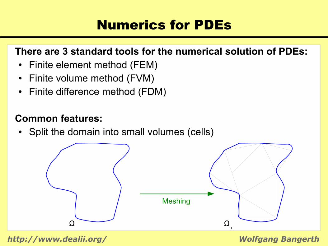
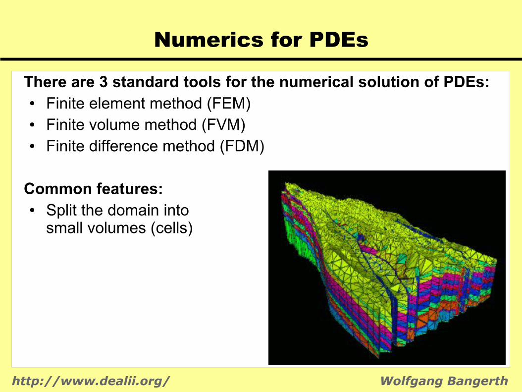
There are 3 standard tools for the numerical solution of PDEs:● Finite element method (FEM)● Finite volume method (FVM)● Finite difference method (FDM)
Common features:● Split the domain into small volumes (cells)
Ω Ωh
Meshing
http://www.dealii.org/ Wolfgang Bangerth
6
Numerics for PDEs
There are 3 standard tools for the numerical solution of PDEs:● Finite element method (FEM)● Finite volume method (FVM)● Finite difference method (FDM)
Common features:● Split the domain into
small volumes (cells)

http://www.dealii.org/ Wolfgang Bangerth
7
Numerics for PDEs
There are 3 standard tools for the numerical solution of PDEs:● Finite element method (FEM)● Finite volume method (FVM)● Finite difference method (FDM)
Common features:● Split the domain into small volumes (cells)● Define balance relations on each cell● Obtain and solve very large (non-)linear systems

http://www.dealii.org/ Wolfgang Bangerth
8
Numerics for PDEs
There are 3 standard tools for the numerical solution of PDEs:● Finite element method (FEM)● Finite volume method (FVM)● Finite difference method (FDM)
Common features:● Split the domain into small volumes (cells)● Define balance relations on each cell● Obtain and solve very large (non-)linear systems
Today and tomorrow: We will not go into details of this, but consider only the parallel computing aspects.
http://www.dealii.org/ Wolfgang Bangerth
9
Numerics for PDEs
Common features:● Split the domain into small volumes (cells)● Define balance relations on each cell● Obtain and solve very large (non-)linear systems
Problems:● Every code has to implement these steps● There is only so much time in a day● There is only so much expertise anyone can have
In addition:● We don't just want a simple algorithm● We want state-of-the-art methods for everything
http://www.dealii.org/ Wolfgang Bangerth
10
Numerics for PDEs
Examples of what we would like to have:● Adaptive meshes● Realistic, complex geometries
● Quadratic or even higher order elements
● Multigrid solvers● Scalability to 1000s of processors● Efficient use of current hardware
● Graphical output suitable for high quality rendering
Q: How can we make all of this happen in a single code?
http://www.dealii.org/ Wolfgang Bangerth
11
How we develop software
Q: How can we make all of this happen in a single code?
Not a question of feasibility but of how we develop software:● Is every student developing their own software?● Or are we re-using what others have done?
● Do we insist on implementing everything from scratch?● Or do we build our software on existing libraries?

http://www.dealii.org/ Wolfgang Bangerth
12
How we develop software
Q: How can we make all of this happen in a single code?
Not a question of feasibility but of how we develop software:● Is every student developing their own software?● Or are we re-using what others have done?
● Do we insist on implementing everything from scratch?● Or do we build our software on existing libraries?
There has been a major shift on how we approach the second question in scientific computing over the past 10-15 years!

http://www.dealii.org/ Wolfgang Bangerth
13
How we develop software
The secret to good scientific software is(re)using existing libraries!

http://www.dealii.org/ Wolfgang Bangerth
14
Existing software
There is excellent software for almost every purpose!
Basic linear algebra (dense vectors, matrices):● BLAS● LAPACK
Parallel linear algebra (vectors, sparse matrices, solvers):● PETSc● Trilinos
Meshes, finite elements, etc:● deal.II – the topic of this class● …
Visualization, dealing with parameter files, ...
http://www.dealii.org/ Wolfgang Bangerth
15
deal.II
deal.II is a finite element library. It provides:
● Meshes
● Finite elements, quadrature,
● Linear algebra
● Most everything you will ever need when writing a finite element code
On the web at
http://www.dealii.org/
http://www.dealii.org/ Wolfgang Bangerth
16
What's in deal.II
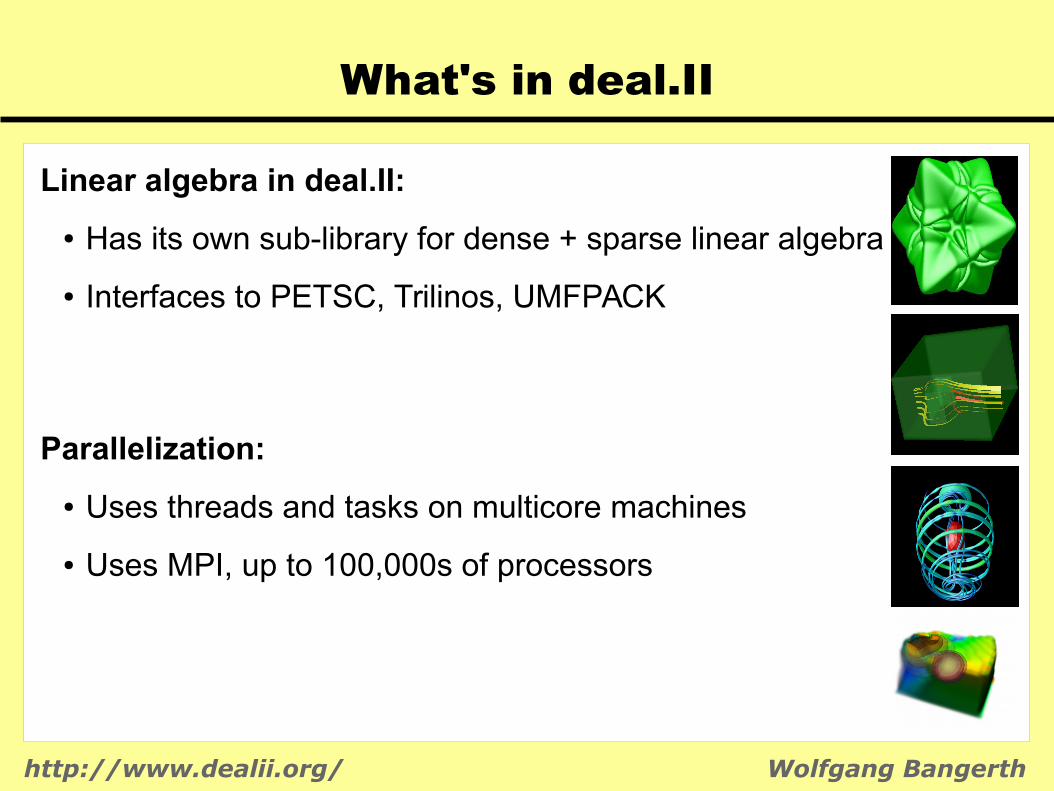
Linear algebra in deal.II:
● Has its own sub-library for dense + sparse linear algebra
● Interfaces to PETSC, Trilinos, UMFPACK
Parallelization:
● Uses threads and tasks on multicore machines
● Uses MPI, up to 100,000s of processors
http://www.dealii.org/ Wolfgang Bangerth
17
On the web
Visit the deal.II library:
http://www.dealii.org/
http://www.dealii.org/ Wolfgang Bangerth
18
deal.II
● Mission: To provide everything that is needed in finite elementcomputations.
● Development:As an open source project
As an inviting community to all who want to contributeAs professional-grade software to users
http://www.dealii.org/ Wolfgang Bangerth
General approach to parallel solvers
Historically, there are three general approaches to solving PDEs in parallel:
● Domain decomposition:– Split the domain on which the PDE is posed– Discretize and solve (small) problems on subdomains– Iterate out solutions
● Global solvers:– Discretize the global problem– Receive one (very large) linear system– Solve the linear system in parallel
● A compromise: Mortar methods
http://www.dealii.org/ Wolfgang Bangerth
Domain decomposition
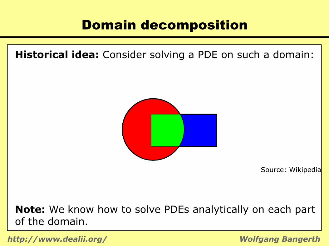
Historical idea: Consider solving a PDE on such a domain:
Source: Wikipedia
Note: We know how to solve PDEs analytically on each part of the domain.

http://www.dealii.org/ Wolfgang Bangerth
Domain decomposition
Historical idea: Consider solving a PDE on such a domain:
Approach (Hermann Schwarz, 1870):● Solve on circle using arbitrary boundary values, get u1
● Solve on rectangle using u1 as boundary values, get u2
● Solve on circle using u2 as boundary values, get u3
● Iterate (proof of convergence: Mikhlin, 1951)
http://www.dealii.org/ Wolfgang Bangerth
Domain decomposition
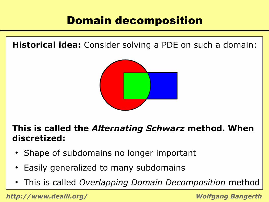
Historical idea: Consider solving a PDE on such a domain:
This is called the Alternating Schwarz method. When discretized:
● Shape of subdomains no longer important
● Easily generalized to many subdomains
● This is called Overlapping Domain Decomposition method
http://www.dealii.org/ Wolfgang Bangerth
Domain decomposition
History's verdict:
● Some beautiful mathematics came of it
● Iteration converges too slowly
● Particularly with large numbers of subdomains (lack of global information exchange)
● Does not play nicely with modern ideas for discretization:– mesh adaptation– hp adaptivity

http://www.dealii.org/ Wolfgang Bangerth
Global solvers
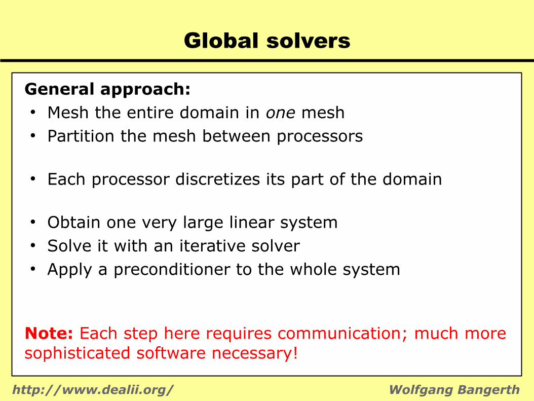
General approach:● Mesh the entire domain in one mesh● Partition the mesh between processors
● Each processor discretizes its part of the domain
● Obtain one very large linear system● Solve it with an iterative solver● Apply a preconditioner to the whole system
http://www.dealii.org/ Wolfgang Bangerth
Global solvers
General approach:● Mesh the entire domain in one mesh● Partition the mesh between processors
● Each processor discretizes its part of the domain
● Obtain one very large linear system● Solve it with an iterative solver● Apply a preconditioner to the whole system
Note: Each step here requires communication; much more sophisticated software necessary!

http://www.dealii.org/ Wolfgang Bangerth
Global solvers
Pros:● Convergence independent of subdivision into subdomains
(if good preconditioner)● Load balancing with adaptivity not a problem● Has been shown to scale to 100,000s of processors
Cons:● Requires much more sophisticated software● Relies on iterative linear solvers● Requires sophisticated preconditioners
But: Powerful software libraries available for all steps.

http://www.dealii.org/ Wolfgang Bangerth
Finite element methods with MPI
Philosophy:● Global objects require O(N) memory (N=# of cells)● Every global data structure needs to be distributed:
– Triangulation– Constraints on the solution– Data attached to cells– Matrix– Solution and right hand side vectors– Postprocessed data (DataOut)
● No processor may hold all data for a global object
● Processors hold O(N/P) “locally owned” data● Processors may also hold O(εN/P) “ghost elements”

http://www.dealii.org/ Wolfgang Bangerth
Finite element methods with MPI
Philosophy:● Every processor may only work on locally owned data
(possibly using ghost data as necessary)
● Software must carefully communicate data that may be necessary early on, try to avoid further communication
● Use PETSc/Trilinos for linear algebra
● (Almost) No handwritten MPI necessary in user code

http://www.dealii.org/ Wolfgang Bangerth
Finite element methods with MPI
Example:● There is an “abstract”, global triangulation● Each processor has a triangulation object that stores
“locally owned”, “ghost” and “artificial” cells (and that's all it knows):
P=0 P=1 P=2 P=3(magenta, green, yellow, red: cells owned by processors 0, 1, 2, 3; blue: artificial cells)

http://www.dealii.org/ Wolfgang Bangerth
Parallel user programs
How user programs need to be modified for parallel computations:
● Need to let– system matrix, vectors– hanging node constraintsknow about what is locally owned, locally relevant
● Need to restrict work to locally owned dataCommunicate everything else on an as-needed basis
● Need to create one output file per processor
● Everything else can happen in libraries under the hood

http://www.dealii.org/ Wolfgang Bangerth
An MPI example: MatVec
Situation:● Multiply a large NxN matrix by a vector of size N● Matrix is assumed to be dense
● Every one of P processors stores N/P rows of the matrix● Every processor stores N/P elements of each vector
● For simplicity: N is a multiple of P
http://www.dealii.org/ Wolfgang Bangerth
An MPI example: MatVec
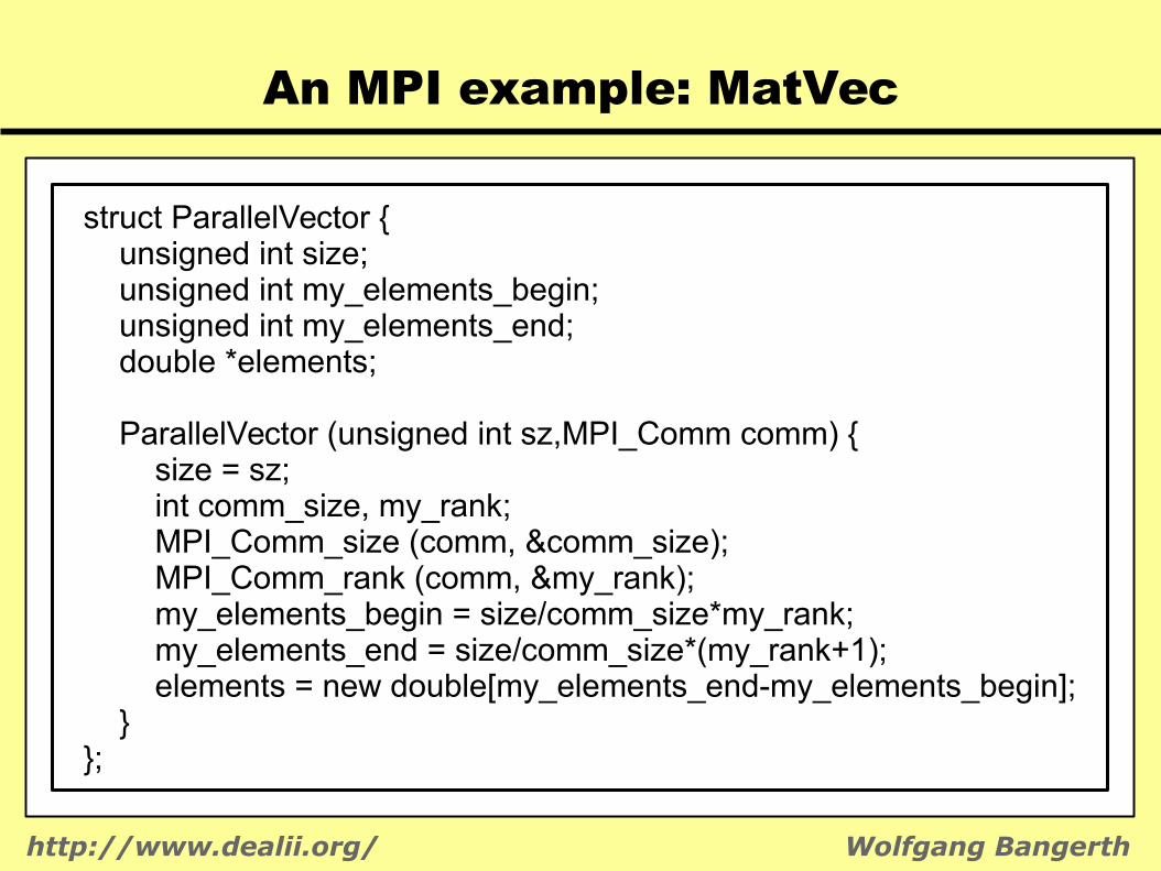
struct ParallelVector { unsigned int size; unsigned int my_elements_begin; unsigned int my_elements_end; double *elements;
ParallelVector (unsigned int sz,MPI_Comm comm) { size = sz; int comm_size, my_rank; MPI_Comm_size (comm, &comm_size); MPI_Comm_rank (comm, &my_rank); my_elements_begin = size/comm_size*my_rank; my_elements_end = size/comm_size*(my_rank+1); elements = new double[my_elements_end-my_elements_begin]; }};

http://www.dealii.org/ Wolfgang Bangerth
An MPI example: MatVec
struct ParallelSquareMatrix { unsigned int size; unsigned int my_rows_begin; unsigned int my_rows_end; double *elements;
ParallelSquareMatrix (unsigned int sz,MPI_Comm comm) { size = sz; int comm_size, my_rank; MPI_Comm_size (comm, &comm_size); MPI_Comm_rank (comm, &my_rank); my_rows_begin = size/comm_size*my_rank; my_rows_end = size/comm_size*(my_rank+1); elements = new double[(my_rows_end-my_rows_begin)*size]; }};
http://www.dealii.org/ Wolfgang Bangerth
An MPI example: MatVec
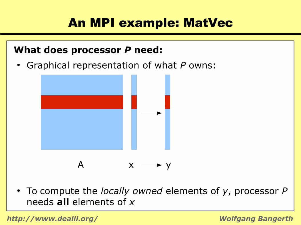
What does processor P need:● Graphical representation of what P owns:
A x y
● To compute the locally owned elements of y, processor P needs all elements of x
http://www.dealii.org/ Wolfgang Bangerth
An MPI example: MatVec
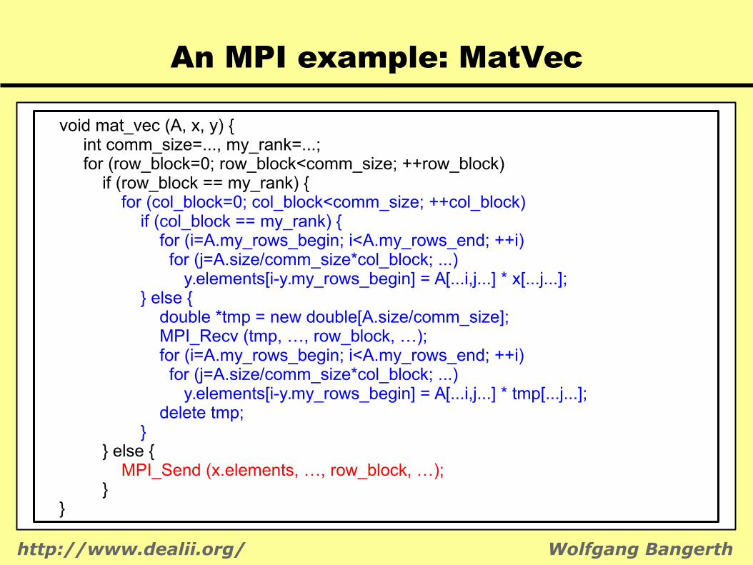
void mat_vec (A, x, y) { int comm_size=..., my_rank=...; for (row_block=0; row_block<comm_size; ++row_block) if (row_block == my_rank) { for (col_block=0; col_block<comm_size; ++col_block) if (col_block == my_rank) { for (i=A.my_rows_begin; i<A.my_rows_end; ++i) for (j=A.size/comm_size*col_block; ...) y.elements[i-y.my_rows_begin] = A[...i,j...] * x[...j...]; } else { double *tmp = new double[A.size/comm_size]; MPI_Recv (tmp, …, row_block, …); for (i=A.my_rows_begin; i<A.my_rows_end; ++i) for (j=A.size/comm_size*col_block; ...) y.elements[i-y.my_rows_begin] = A[...i,j...] * tmp[...j...]; delete tmp; } } else { MPI_Send (x.elements, …, row_block, …); }}

http://www.dealii.org/ Wolfgang Bangerth
An MPI example: MatVec
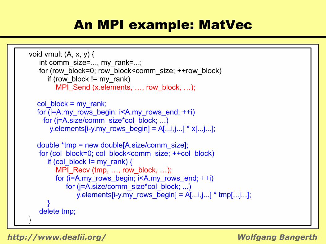
Analysis of this algorithm● We only send data right when we need it:
– receiving processor has to wait– has nothing to do in the meantimeA better algorithm would:– send out its data to all other processors– receive messages as needed (maybe already here)
● As a general rule:– send data as soon as possible– receive it as late as possible– try to interleave computations between sends/receives
● We repeatedly allocate/deallocate memory – should set up buffer only once
http://www.dealii.org/ Wolfgang Bangerth
An MPI example: MatVec
void vmult (A, x, y) { int comm_size=..., my_rank=...; for (row_block=0; row_block<comm_size; ++row_block) if (row_block != my_rank) MPI_Send (x.elements, …, row_block, …); col_block = my_rank; for (i=A.my_rows_begin; i<A.my_rows_end; ++i) for (j=A.size/comm_size*col_block; ...) y.elements[i-y.my_rows_begin] = A[...i,j...] * x[...j...];
double *tmp = new double[A.size/comm_size]; for (col_block=0; col_block<comm_size; ++col_block) if (col_block != my_rank) { MPI_Recv (tmp, …, row_block, …); for (i=A.my_rows_begin; i<A.my_rows_end; ++i) for (j=A.size/comm_size*col_block; ...) y.elements[i-y.my_rows_begin] = A[...i,j...] * tmp[...j...]; } delete tmp;}
http://www.dealii.org/ Wolfgang Bangerth
Message Passing Interface (MPI)
Notes on using MPI:● Usually, algorithms need data that resides elsewhere● Communication needed
● Distributed computing lives in the conflict zone between– trying to keep as much data available locally to avoid communication– not creating a memory/CPU bottleneck
● MPI makes the flow of information explicit● Forces programmer to design data structures/algorithms
for communication
● Well written programs have relatively few MPI calls

http://www.dealii.org/ Wolfgang Bangerth
Solver questions
The finite element method provides us with a linear system
We know:● A is large: typically a few 1,000 up to a few billions● A is sparse: typically no more than a few 100 entries per
row● A is typically ill-conditioned: condition numbers up to 109
Question:How do we go about solving
such linear systems?
A x = b

http://www.dealii.org/ Wolfgang Bangerth
Direct solvers
Direct solvers – compute a decomposition of A:● Can be thought of as variant of LU decomposition that
finds triangular factors L, U so that
● Sparse direct solvers save memory and CPU time by considering the sparsity pattern of A
● Very robust● Work grows as O(N1+2(d-1)/d), i.e.,
– O(N2) in 2d– O(N7/3) in 3d
● Memory grows as O(N1+(d-1)/d), i.e., – O(N3/2) in 2d– O(N5/3) in 3d
A = LU

http://www.dealii.org/ Wolfgang Bangerth
Direct solvers
Where to get a direct solver:● Several very high quality, open source packages● Most widely used ones are
- UMFPACK- SuperLU- MUMPS
● The latter two are even parallelized
But:
It is generally very difficult to implementdirect solvers efficiently in parallel.

http://www.dealii.org/ Wolfgang Bangerth
Iterative solvers
Iterative solvers improve the solution in each iteration:
● Start with an initial guess x0
● Continue iterations till a stopping criterion is satisfied(typically that the error/residual is less than a tolerance)
● Return final guess xk
● Depending on solver and preconditioner type, work can be O(N) or (much) worse
● Memory is typically linear, i.e., O(N)
Note: The final guess does not solve Ax=b exactly!

http://www.dealii.org/ Wolfgang Bangerth
Iterative solvers
There is a wide variety of iterative solvers:
● CG, MinRes, GMRES, …
● All of them are actually rather simple to implement:They usually need less than 200 lines of code
● Consequently, many high quality implementations
Advantage: Only need multiplication with the matrix, no modification/insertion of matrix elements required.
Disadvantage: Efficiency hinges on availability of good preconditioners.

http://www.dealii.org/ Wolfgang Bangerth
Direct vs iterative
Guidelines for direct solvers vs iterative solvers:
Direct solvers:✔ Always work, for any invertible matrix✔ Faster for problems with <100k unknowns✗ Need too much memory + CPU time for larger problems✗ Do not parallelize well
Iterative solvers:✔ Need O(N) memory✔ Can solve very large problems✔ Often parallelize well✗ Choice of solver/preconditioner depends on problem
http://www.dealii.org/ Wolfgang Bangerth
Advice for iterative solvers
There is a wide variety of iterative solvers:● CG: Conjugate gradients● MinRes: Minimal residuals● GMRES: Generalized minimal residuals● F-GMRES: Flexible GMRES● SymmLQ: Symmetric LQ decomposition● BiCGStab: Biconjugate gradients stabilized● QMR: Quasi-minimal residual● TF-QMR: Transpose-free QMR● …
Which solver to choose depends on the propertiesof the matrix, primarily symmetry and definiteness!

http://www.dealii.org/ Wolfgang Bangerth
Advice for iterative solvers
Guidelines for use:● CG: Matrix is symmetric, positive definite● MinRes: –● GMRES: Catch-all● F-GMRES: Catch-all with variable preconditioners● SymmLQ: –● BiCGStab: Matrix is non-symmetric but positive definite● QMR: –● TF-QMR: – ● All others: –
In reality, only CG, BiCGStab and (F-)GMRESare used much.
http://www.dealii.org/ Wolfgang Bangerth
Advice for iterative solvers
Note:
All iterative solvers are badwithout a good preconditioner!
The art of devising a good iterative solveris to devise a good preconditioner!

http://www.dealii.org/ Wolfgang Bangerth
Observations on iterative solvers
The finite element method provides us with a linear system
that we then need to solve.
Basic observations:● For sparse direct solvers, speed of solution only depends
on sparsity pattern● For iterative solvers, performance also depends on the
values in A● Performance measures:
– number of iterations– cost of every iteration
A x = b

http://www.dealii.org/ Wolfgang Bangerth
Observations on iterative solvers
The finite element method provides us with a linear system
that we then need to solve.
Factors affecting performance of iterative solvers:● Symmetry of a matrix● Whether A is definite● Condition number of A● How the eigenvalues of A are clustered
● Whether A is reducible/irreducible
A x = b

http://www.dealii.org/ Wolfgang Bangerth
Observations on iterative solvers
Example 1: Using CG to solve
where A is SPD, each iteration reduces the residual by a factor of
● For a tolerance ε we need iterations
● Problem: The condition number typically grows with the problem size number of iterations grows→
A x = b
r = √ κ(A )−1
√ κ(A )+1 < 1
n = log ϵlog r

http://www.dealii.org/ Wolfgang Bangerth
Observations on iterative solvers
Example 2: When solving
where A has the form
then every decent iterative solver converges in 1 iteration.
Note 1: This, even though condition number may be largeNote 2: This is true, in particular, if A=I.
A x = b
A = (a11 0 0 ⋯0 a22 0 ⋯0 0 a33 ⋯⋮ ⋮ ⋮ ⋱
)
http://www.dealii.org/ Wolfgang Bangerth
The idea of preconditioners
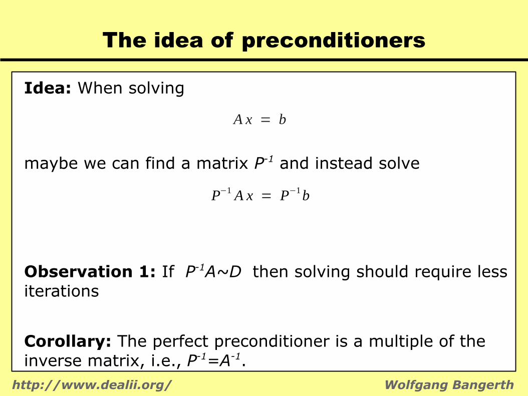
Idea: When solving
maybe we can find a matrix P-1 and instead solve
Observation 1: If P-1A~D then solving should require less iterations
Corollary: The perfect preconditioner is a multiple of the inverse matrix, i.e., P-1=A-1.
A x = b
P−1 A x = P−1b

http://www.dealii.org/ Wolfgang Bangerth
The idea of preconditioners
Idea: When solving
maybe we can find a matrix P-1 and instead solve
Observation 2: Iterative solvers only need matrix-vector multiplications, no element-by-element access.
Corollary: It is sufficient if P-1 is just an operator
A x = b
P−1 A x = P−1b

http://www.dealii.org/ Wolfgang Bangerth
The idea of preconditioners
Idea: When solving
maybe we can find a matrix P-1 and instead solve
Observation 3: There is a tradeoff:fewer iterations vs cost of preconditioner.
Corollary: Preconditioning only works if P-1 is cheap to compute and if P-1 is cheap to apply to a vector.
Consequence: P-1=A-1 does not qualify.
A x = b
P−1 A x = P−1b

http://www.dealii.org/ Wolfgang Bangerth
The idea of preconditioners
Notes on the following lectures:● For quantitative analysis, one typically needs to consider
the spectrum of operators and preconditioners
● Here, the goal is simply to get an “intuition” on how preconditioners work
http://www.dealii.org/ Wolfgang Bangerth
Constructing preconditioners
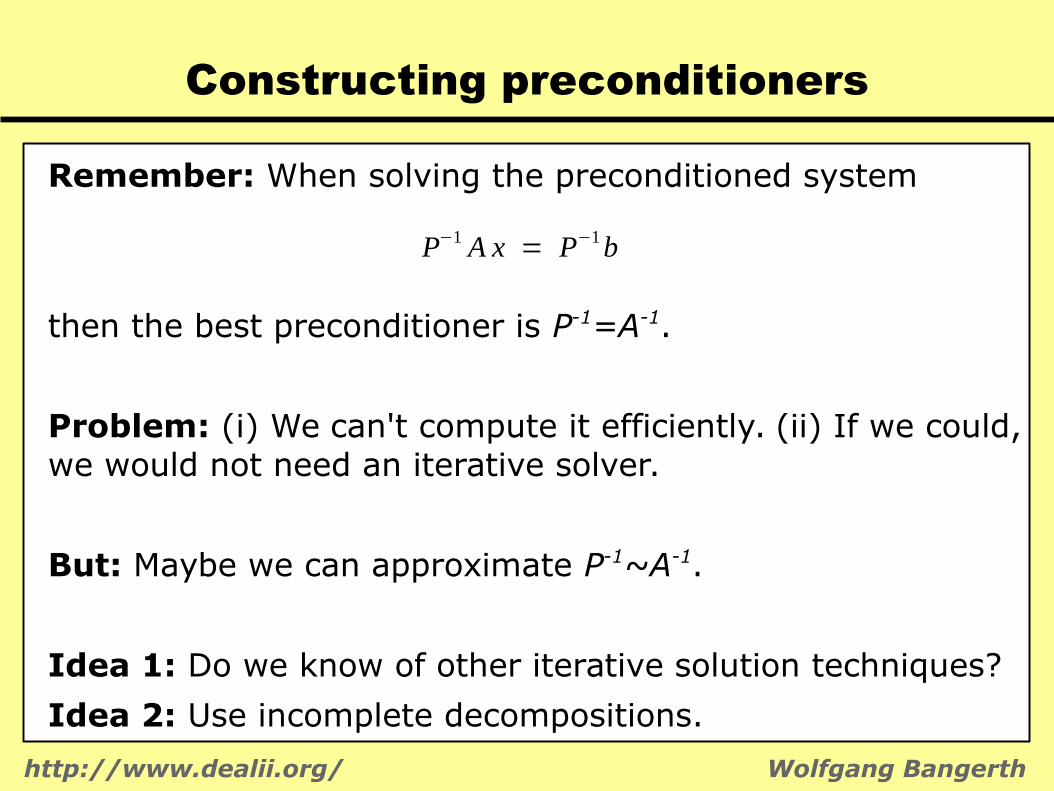
Remember: When solving the preconditioned system
then the best preconditioner is P-1=A-1.
Problem: (i) We can't compute it efficiently. (ii) If we could, we would not need an iterative solver.
But: Maybe we can approximate P-1~A-1.
Idea 1: Do we know of other iterative solution techniques?
Idea 2: Use incomplete decompositions.
P−1 A x = P−1b

http://www.dealii.org/ Wolfgang Bangerth
Constructing preconditioners
Approach 1: Remember the oldest iterative techniques!
To solve we can use defect correction:● Under certain conditions, the iteration:
will converge to the exact solution x
● Unlike Krylov-space methods, convergence is linear● The best preconditioner is again P-1~A-1
x(k+1) = x(k )−P−1(A x(k )−b)
A x = b

http://www.dealii.org/ Wolfgang Bangerth
Constructing preconditioners
Approach 1: Remember the oldest iterative techniques!
Preconditioned defect correction for :● Jacobi iteration:
● The Jacobi preconditioner is then
which is easy to compute and apply.
Note: We don't need the scaling (“relaxation”) factor.
x(k+1) = x(k )−ω D−1(A x(k )−b)
Ax = b , A = L+D+U
P−1 = ω D−1

http://www.dealii.org/ Wolfgang Bangerth
Constructing preconditioners
Approach 1: Remember the oldest iterative techniques!
Preconditioned defect correction for :● Gauss-Seidel iteration:
● The Gauss-Seidel preconditioner is then
which is easy to compute and apply as L+D is triangular.
Note 1: We don't need the scaling (“relaxation”) factor.Note 2: This preconditioner is not symmetric.
x(k+1) = x(k )−ω(L+D)−1(A x(k )−b)
Ax = b , A = L+D+U
P−1 = ω(L+D)−1 i.e. h=P−1r solves (L+D)h=ωr

http://www.dealii.org/ Wolfgang Bangerth
Constructing preconditioners
Approach 1: Remember the oldest iterative techniques!
Preconditioned defect correction for :● SOR (Successive Over-Relaxation) iteration:
● The SOR preconditioner is then
Note 1: This preconditioner is not symmetric.Note 2: We again don't care about the constant factor in P.
x(k+1) = x(k )−ω(D+ωL)−1(A x(k )−b)
Ax = b , A = L+D+U
P−1 = (D+ω L)−1

http://www.dealii.org/ Wolfgang Bangerth
Constructing preconditioners
Approach 1: Remember the oldest iterative techniques!
Preconditioned defect correction for :● SSOR (Symmetric Successive Over-Relaxation) iteration:
● The SSOR preconditioner is then
Note: This preconditioner is now symmetric if A is symmetric!
x(k+1) = x(k )− 1ω(2−ω)
(D+ωU )−1 D(D+ωL)−1(A x(k )−b)
Ax = b , A = L+D+U
P−1 = (D+ωU )−1 D(D+ωL)−1

http://www.dealii.org/ Wolfgang Bangerth
Constructing preconditioners
Approach 1: Remember the oldest iterative techniques!
Common observations about preconditioners from stationary iterations:
● Have been around for a long time
● Generally useful for small problems (<100,000 DoFs)
● Not particularly useful for larger problems
http://www.dealii.org/ Wolfgang Bangerth
Constructing preconditioners
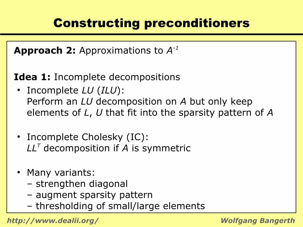
Approach 2: Approximations to A-1
Idea 1: Incomplete decompositions● Incomplete LU (ILU):
Perform an LU decomposition on A but only keep elements of L, U that fit into the sparsity pattern of A
● Incomplete Cholesky (IC):LLT decomposition if A is symmetric
● Many variants:– strengthen diagonal– augment sparsity pattern– thresholding of small/large elements
Note: This preconditioner is again symmetric.
http://www.dealii.org/ Wolfgang Bangerth
Summary
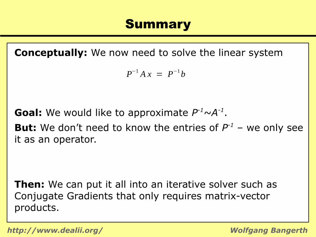
Conceptually: We now need to solve the linear system
Goal: We would like to approximate P-1~A-1.
But: We don’t need to know the entries of P-1 – we only see it as an operator.
Then: We can put it all into an iterative solver such as Conjugate Gradients that only requires matrix-vector products.
P−1 A x = P−1b
http://www.dealii.org/ Wolfgang Bangerth
Global solvers
Examples for a few necessary steps:● Matrix-vector products in iterative solvers
(Point-to-point communication)
● Dot product synchronization
● Available parallel preconditioners

http://www.dealii.org/ Wolfgang Bangerth
Matrix-vector product
What does processor P need:● Graphical representation of what P owns:
A x y
● To compute the locally owned elements of y, processor P needs all elements of x
● All processors need to send their share of x to everyone
http://www.dealii.org/ Wolfgang Bangerth
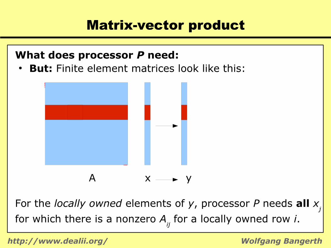
Matrix-vector product
What does processor P need:● But: Finite element matrices look like this:
A x y
For the locally owned elements of y, processor P needs all xj
for which there is a nonzero Aij for a locally owned row i.

http://www.dealii.org/ Wolfgang Bangerth
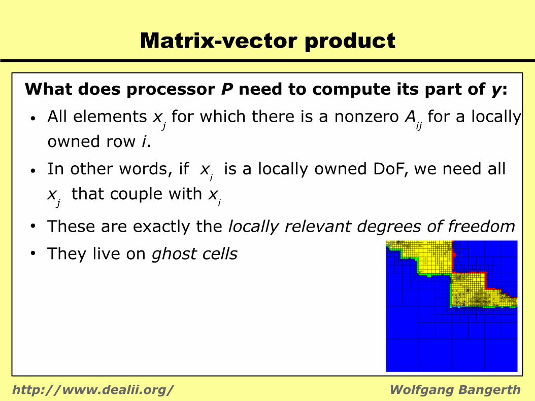
Matrix-vector product
What does processor P need to compute its part of y:
● All elements xj for which there is a nonzero A
ij for a locally
owned row i.
● In other words, if xi is a locally owned DoF, we need all
xj that couple with x
i
● These are exactly the locally relevant degrees of freedom● They live on ghost cells
http://www.dealii.org/ Wolfgang Bangerth
Matrix-vector product
What does processor P need to compute its part of y:
● All elements xj for which there is a nonzero A
ij for a locally
owned row i.
● In other words, if xi is a locally owned DoF, we need all
xj that couple with x
i
● These are exactly the locally relevant degrees of freedom● They live on ghost cells

http://www.dealii.org/ Wolfgang Bangerth
Matrix-vector product
Parallel matrix-vector products for sparse matrices:● Requires determining which elements
we need from which processor● Exchange this up front once
Performing matrix-vector product:● Send vector elements to all processors
that need to know● Do local product (dark red region)● Wait for data to come in● For each incoming data packet, do
nonlocal product (light red region)Note: Only point-to-point comm. needed!
http://www.dealii.org/ Wolfgang Bangerth
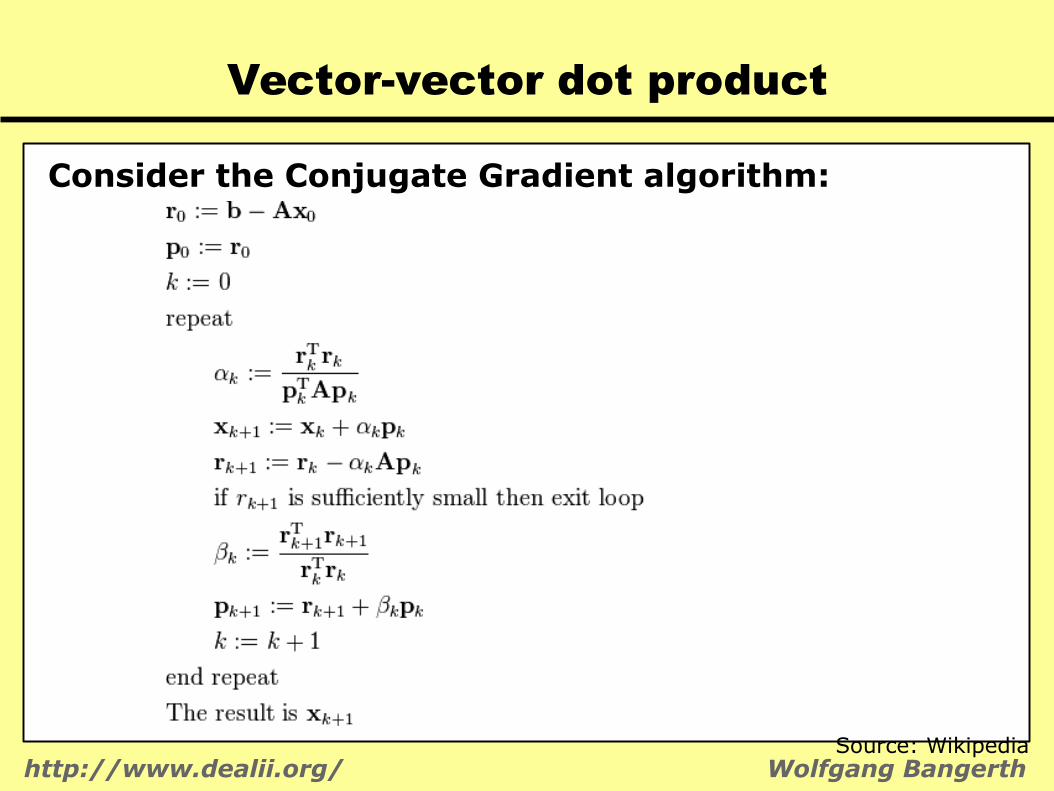
Vector-vector dot product
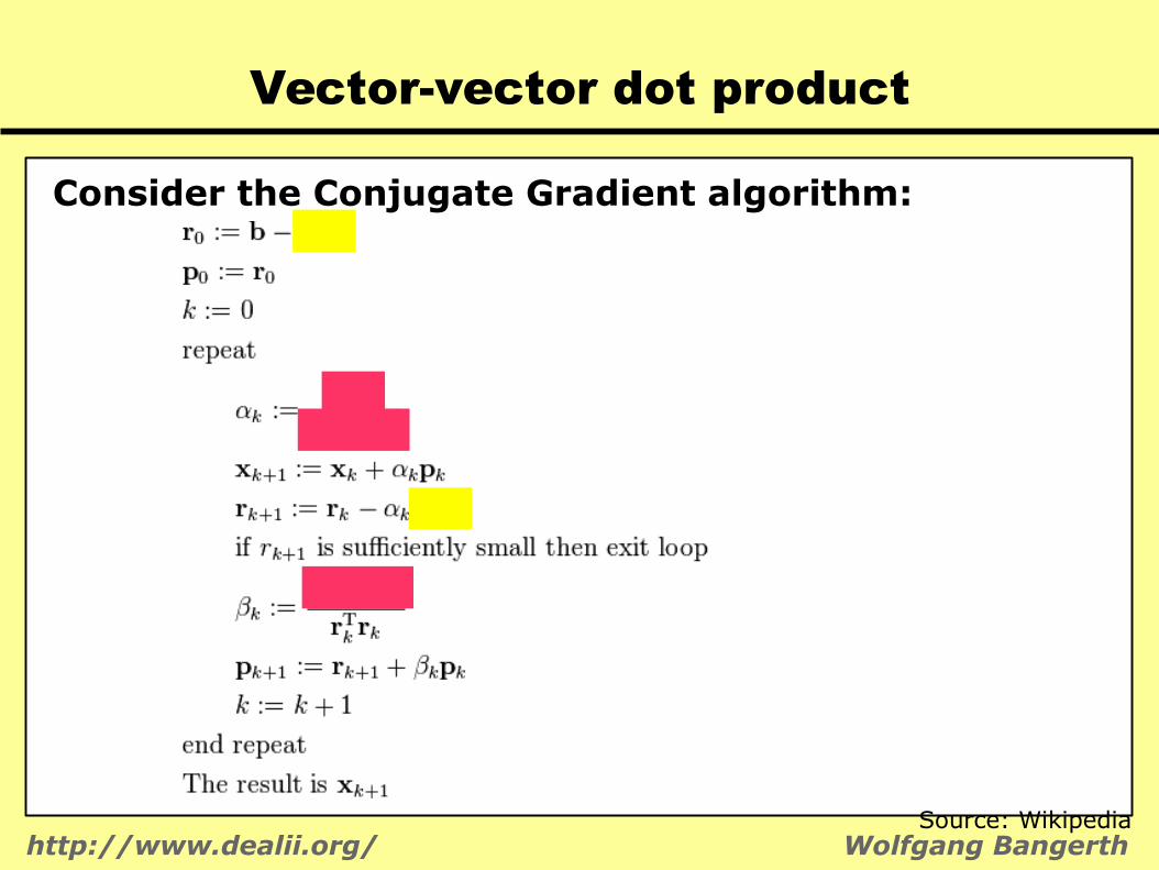
Consider the Conjugate Gradient algorithm:
Source: Wikipedia
http://www.dealii.org/ Wolfgang Bangerth
Vector-vector dot product
Consider the Conjugate Gradient algorithm:
Source: Wikipedia

http://www.dealii.org/ Wolfgang Bangerth
Vector-vector dot product
Consider the dot product:
x⋅y = ∑i=1
Nxi y i = ∑p=1
P
(∑local elements on proc pxi y i)
http://www.dealii.org/ Wolfgang Bangerth
Parallel considerations
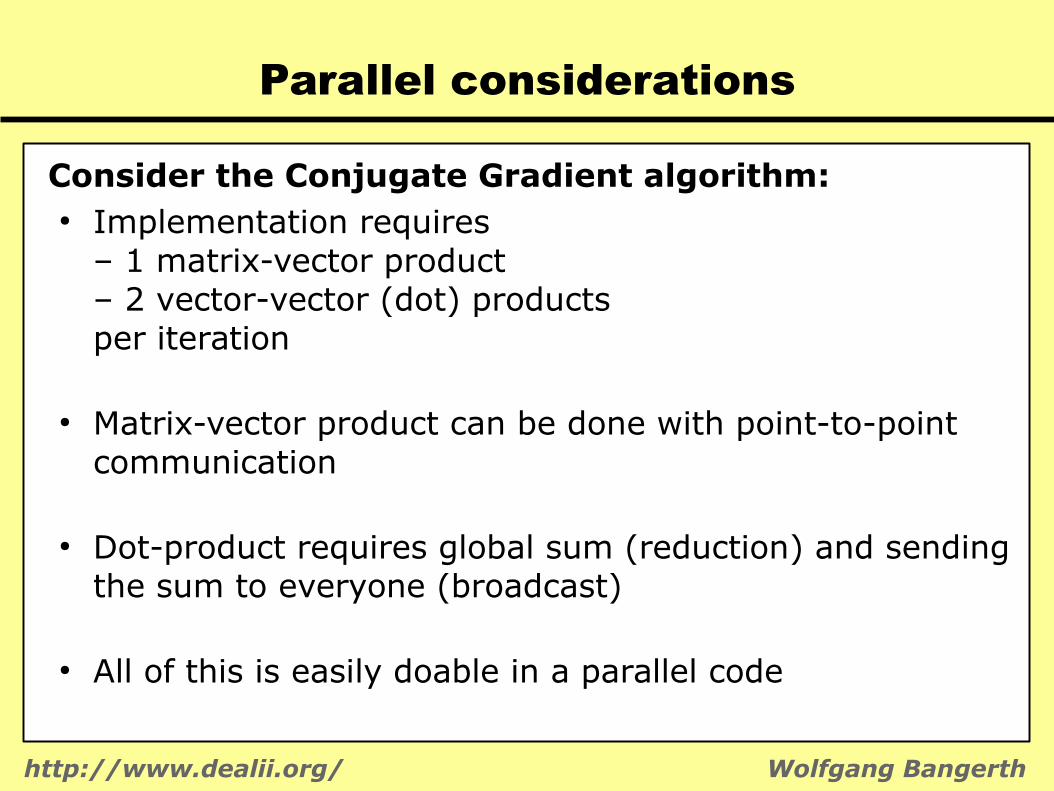
Consider the Conjugate Gradient algorithm:● Implementation requires
– 1 matrix-vector product– 2 vector-vector (dot) productsper iteration
● Matrix-vector product can be done with point-to-point communication
● Dot-product requires global sum (reduction) and sending the sum to everyone (broadcast)
● All of this is easily doable in a parallel code

http://www.dealii.org/ Wolfgang Bangerth
Parallel preconditioners
Consider Krylov-space methods algorithm:To solve Ax=b we need
● Matrix-vector products z=Ay● Various vector-vector operations● A preconditioner v=Pw
● Want: P approximates A-1
Question: What are the issues in parallel?

http://www.dealii.org/ Wolfgang Bangerth
Parallel preconditioners
First idea: Block-diagonal preconditioners
Pros:● P can be computed locally● P can be applied locally (without communication)● P can be approximated (SSOR, ILU on each block)
Cons:● Deteriorates with larger numbers
of processors● Equivalent to Jacobi in the extreme
of one row per processor
Lesson: Diagonal block preconditionersdon't work well! We need data exchange!
http://www.dealii.org/ Wolfgang Bangerth
Parallel preconditioners
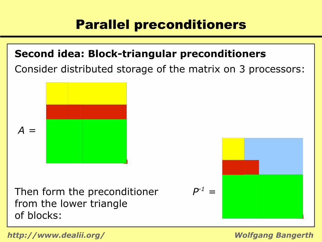
Second idea: Block-triangular preconditioners
Consider distributed storage of the matrix on 3 processors:
A =
Then form the preconditioner P-1 =from the lower triangleof blocks:

http://www.dealii.org/ Wolfgang Bangerth
Parallel preconditioners
Second idea: Block-triangular preconditioners
Pros:● P can be computed locally● P can be applied locally● P can be approximated (SSOR, ILU on each block)● Works reasonably well
Cons:● Equivalent to Gauss-Seidel in the
extreme of one row per processor● Is sequential!
Lesson: Data flow must have fewer then O(#procs) synchronization points!

http://www.dealii.org/ Wolfgang Bangerth
Parallel preconditioners
What works:● Geometric multigrid methods for elliptic problems:
– Require point-to-point communication in smoother– Very difficult to load balance with adaptive meshes– O(N) effort for overall solver
● Algebraic multigrid methods for elliptic problems:– Require point-to-point communication . in smoother . in construction of multilevel hierarchy– Difficult (but easier) to load balance– Not quite O(N) effort for overall solver
– “Black box” implementations available (ML, hypre)

http://www.dealii.org/ Wolfgang Bangerth
Parallel preconditioners
Examples (strong scaling):
Laplace equation (from Bangerth et al., 2011)

http://www.dealii.org/ Wolfgang Bangerth
Parallel preconditioners
Examples (strong scaling):
Elasticity equation (from Frohne, Heister, Bangerth, submitted)
http://www.dealii.org/ Wolfgang Bangerth
Parallel preconditioners
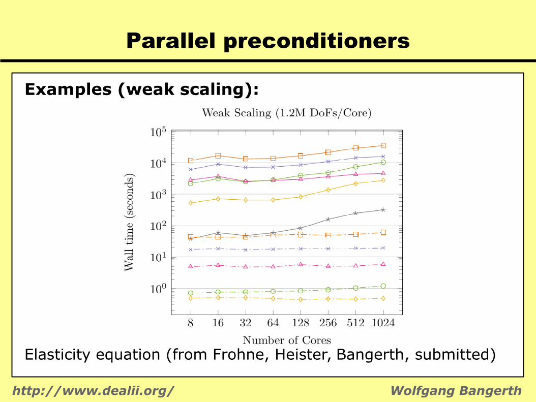
Examples (weak scaling):
Elasticity equation (from Frohne, Heister, Bangerth, submitted)

http://www.dealii.org/ Wolfgang Bangerth
Parallel solvers
Summary:
● Mental model: See linear system as a large whole
● Apply Krylov-solver at the global level
● Use algebraic multigrid method (AMG) as black box preconditioner for elliptic blocks
● Build more complex preconditioners for block systems(see lecture 38)
● Might also try parallel direct solvers