Embed Size (px)
Citation preview

Finite Element Analysis
Prof. Dr. B. N. Rao
Department of Civil Engineering
Indian Institute of Technology, Madras
Module - 01
Lecture - 11
Last class, what we did is, we looked at a method called superposition method for
handling beam subjected to uniformly distributed loads. Using one finite element, we can
get exact solution. As I mentioned, the problem with the finite element formulation that
we developed is – it gives exact solutions for displacements and rotations at the nodes.
So, this gives accurate solutions for beam subjected to concentrated loads. When beam is
subjected to distributed loads, when you apply this finite element formulation, it gives
exact solutions of displacements and rotations at the nodes. However, when you try to
calculate moments, shear or in fact, displacement at any other point along the length of
the beam, the solution may not be accurate. So, one way of handling this is, to increase
the number of finite elements, so that we approach the exact solution as we increase the
number of elements. However, that is not smart way of doing. The other way of handling
the situation is, you use a method what is called a superposition method, which we
discussed in the last class.
I want to just highlight what we have done in superposition method. In superposition
method, the solution procedure is like this – we can write the element equations and
assemble the element equations to get the global equations, and solve them in the usual
manner. So, if a beam continuous beam is given with distributed loads, you just proceed
as you do regularly; that is, you get the element equations and based on the element
connectivity, you assemble the global equations, then apply the boundary conditions, and
solve these equations, and get the nodal values. So, in superposition method, up to that
point it is same. After that, when you are computing the element quantities, that is,
displacement at any point in an element using the nodal values, or moment at any point
in an element, or shear at any point in an element using the nodal values, what you need
to do is, you superpose the exact solution of fixed-end beam problem – means – imagine
in this continuous beam, each of the span is fixed. Get the fixed-end moment solutions

and you superpose those on the solution that you got from finite elements. So, that gives
you the correction; that is, superposition of fixed moments act like a correction and you
will be able to get exact solution even with less number of elements – in fact, even one
element.
(Refer Slide Time: 03:48)
Here it goes like this – displacement at any point in the element. Here you have two
terms. The first term is nothing but what you do by using the nodal values v1, theta 1, v2,
theta 2 – you interpolate using finite element shape functions. To that, you are adding the
second term. The second term is coming from fixed-end solution. This fixed-end solution
corresponds to the problem of uniformly distributed load over the span. So, this is the
correction term. You will not be having this term if it is a point load problem, because
you do not need to apply this correction term. This formula is coming from superposition
method.

(Refer Slide Time: 04:49)
Next, bending moment at any point in the element is as usual. You can interpolate using
the nodal values and over that you superposed fixed-end moment solution. Similarly, for
shear.
(Refer Slide Time: 05:09)
Shear force at any point in the element is given by this one. The first term is nothing but
interpolation of the nodal values as you do for any other problem with concentrated
loads. The second term is the correction term for the distributed load case. As I
mentioned, all these correction terms here are corresponding to uniformly distributed

load – fixed beam with uniformly distributed. If you have some other loading, you need
to add the fixed-end moments corresponding to that loading, imagining that each span of
the continuous beam is fixed.
Now, let us take an example – we will take the same example as what we have seen
earlier; that is, uniformly distributed load; simply supported beam with uniformly
distributed load – length of the beam is L. Earlier, we solved using two finite elements
and we observed that end shear and mid-span moments are not matching with the exact
solution. Then, what we did is, we started out discussing about the superposition method.
Now, let us go back to the same problem. As I mentioned, even with one element, you
will be able get exact solution.
(Refer Slide Time: 06:55)
Let us see how it is possible using the superposition method. This is a simply supported
beam subjected to uniformly distributed load, having span L and modulus of rigidity EI –
it is constant. We are assuming a prismatic beam and uniformly distributed load. This
entire beam is discretized using one element having length L. The nodal degrees of
freedom are v1, theta 1, v2, theta 2.
Element solutions – you know that there are no point loads or concentrated loads. So,
element solutions look like this (Refer Slide Time: 07:37). Now, since we use only one
element, this also becomes a global equation. Now, we need to apply the displacement

boundary conditions. Displacement boundary conditions here are: node 1 is fixed in the
transverse direction; node 2 is not fixed, actually, displacement in the transverse
direction is restrained. So, v1 is 0; v2 is 0.
(Refer Slide Time: 08:21)
Wherever essential boundary conditions are 0, reactions will be developed at those
locations. So, we get this equation system. Substituting v1 is equal to 0, v2 is equal to 0,
and the corresponding locations in the force vector are replaced with reaction R1 and
reaction R2. Since v1 and v2 are 0, we can eliminate rows and columns corresponding to
those locations. So, we can eliminate 1 and 3 rows and columns. We get the reduced
equation system by eliminating 1 and 3 rows and columns, which we can solve for theta
1 and theta 2. The solution is this one.
Now, since we got all the nodal values, that is, we know what is v1 and now, we
calculate at theta 1. Similarly, we know what is v2 and now, we calculate at theta 2.
Now, we are ready to solve for the element quantities – element quantities like
displacement at any point in the element; moment at any point in the element; shear at
any point in the element.

(Refer Slide Time: 09:55)
Displacement at any point in the element; using these nodal values – v 1, theta 1, v2,
theta 2, we can interpolate using finite element shape functions. The first term is nothing
but interpolation of using finite elemental shape functions and the second term is coming
from fixed-end moment displacement. These fixed-end moment values can be obtained
readily in any of the elementary strength of materials or mechanics of materials books.
(Refer Slide Time: 10:36)
Now, we have the nodal values and also we know the correction term. So, we can
simplify this further and we get this one. If you want mid-span displacement, since we

have taken only one element, we need to substitute s is equal to 0.5. Mid-span
displacement – we evaluated at S is equal to half; that is, 0.5 – is this one. Please
remember – this value we got after applying the fixed-end moment correction. If we miss
that correction term, this may not be the value that will be getting. This is the exact
solution.
(Refer Slide Time: 11:33)
Now, bending moment at any point using the nodal values and second derivative of
shape functions interpolating; using the second derivative of shape functions and the
nodal values, we will get the first term. The second term is nothing but it is coming from
the fixed-end solution, which acts like a correction term. Now, simplifying this in the
maximum bending moment because last time, when we did the comparisons between the
solutions that we got from finite elements, using two elements and the exact solution,
what we did is, we compared mid-span displacement or mid-span moments and shear.
So, maximum moment is going to occur at mid-span. Mid-span moment is obtained by
substituting s is equal to again 0.5. This is M moment expression – simplified.

(Refer Slide Time: 12:58)
Now, maximum bending moment occurs at the mid-span, which is obtained by
substituting s is equal to half; we get this value, which now matches with exact solution,
because we applied fixed-end moment correction.
(Refer Slide Time: 13:34)
Again, shear at any point; substituting the nodal values v1, theta 1, v2, theta 2, we get
this one. Again, first term is nothing but it consists of third derivative of shape functions
and the nodal values. The second term is nothing but fixed-end solution for uniformly
distributed load case. Once we apply this correction term, we get shear like this. Shear at

the ends of the span; we get by substituting s is equal to 0 or s is equal to 1. So,
maximum shear is at the end and can be obtained by setting s is equal to 0 in the equation
for shear force, and we get the value minus q L over 2, which now matches with exact
solution.
Once again I want to emphasize that the effect of the superposition method is – proceed
in the usual manner of writing element equations, assemble them to get the global
equations, and solve for the nodal unknowns. Then, when computing the element
quantities, the exact solution of fixed-end beam problem is added to the finite element
solution. So, this is the procedure, which we verify by taking simply supported beam
subjected to uniformly distributed load. We check that with exact solution – they are
matching. When we apply the superposition method, the same problem when we solved
with two finite elements, there is some inaccuracy. One way of handling it is to increase
the number of elements, but that is not smart way of doing things. So, we will be
adopting superposition methods whenever we have distributed load in any span of a
beam.
(Refer Slide Time: 15:57)
Now, let us take an example – three span continuous beam. Find deflections, moments
and shears in a continuous beam shown in figure. The material properties, Young’s
modulus and cross sectional properties, moment of inertia – all are given in SI units.
Earlier also, we have seen similar kind of continuous beam except that there we have

point load; at the middle of the mid-span, we have a point load earlier of 8 kilo Newton
at a location, which is middle of mid-span. Now, the only difference is, in the mid-span,
we have distributed load of 20 kilo Newton per mm. Similar to what we did earlier, what
we can do is – since this problem is symmetric with respect to the mid-point, we can take
advantage of symmetry of this problem and only model half of this continuous beam.
Please note that at the supports, the transverse displacement is 0 and the rotation is 0 at
the middle of mid-span.
(Refer Slide Time: 17:47)
Using symmetry, only half of the beam can be modeled. The two element model looks
like this. In the half model – half of that continuous three span continuous beam model –
when you take half of that, in the first span or if you look at this half model, we have
three supports. So, we use nodes, one at each support and we get this. Minimum we can
use is two elements. The displacements restrains are shown here in the half model. We
already did similar kind of exercise for this kind of three span continuous beam earlier,
with a point load. So, the first element degrees of freedom are v1, theta 1, v2, theta 2;
second element degrees of freedom are v2, theta 2, v3, theta 3.
The global stiffness matrix for this example is similar to the global stiffness matrix for
three span continuous beam. We have seen earlier, subjected to point load – stiffness
matrix remains same because span is same, and also, material properties and cross
sectional properties are same. Only difference will be the load vector or equivalent nodal
load vector, because earlier we had a point load and now, we have a distributed load. So,
what we will do is – since we already solved this kind of problem, we will take the
stiffness matrices from the previous calculations. Now, let us concentrate only on the
equivalent load vector for each of the element and assemble the global load vector. If
you see element one, there is no load applied; or, in the first span of 400 millimeters,
there is no load applied.
(Refer Slide Time: 20:16)
Load vector for element 1 is going to be this. Load vector for element 2 – element 2 is
having a distributed load of 20 kilo Newton per millimeter; also, the span of this second
element or length of second element is 200 millimeters. So, the load vector for element
2, we can obtain by substituting into the formula that we developed for the case of
uniformly distributed load. Please note that this formula is valid only if q is constant; that
is, q is uniformly distributed. Since our case here – q is uniformly distributed; that is,
value is 20 newton per millimeter, we can directly use this formula – substitute q is equal
to 20 Newton per millimeter, L is equal to 200 millimeters, and do the computations, we
get this.
The global load vector – here, we have three nodes. At each node, we have 2 degrees of
freedom. Element 1 contribution goes into 1 2 3 4 locations of rows and columns, and
element 2 contribution goes into 3 4 5 6 rows and columns or element 1 contribution
goes into 1 2 3 4 locations of the global force vector, and element 2 contribution goes
into 3 4 5 6 locations of the global force vector. So, we get global load vector from these
element load vector.
(Refer Slide Time: 22:16)
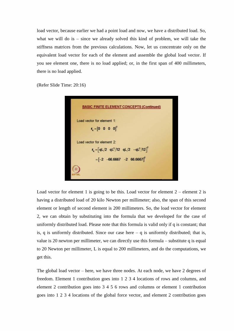
Also, please note that v1 is transverse displacement at node 1 is restrained; v1 is 0.
Similarly, transverse displacement at node 2 is restrained; v2 is 0; because of symmetry,
rotation at node 3 is 0. So, at this corresponding locations in the global load vector,
reactions will be developed, which are a denoted with R1, R2 and M3 – these we do not
know now; we need to determine later. So, these are unknown reactions. So, we got the
global load vector. As I mentioned, the global stiffness matrix for this problem, we can
take it from the earlier, when we solve this problem with point load; from there we can
take it.

(Refer Slide Time: 23:26)
The complete set of global equations look like this. Now, as usual eliminating the rows
and columns corresponding to the degrees of freedom, which are 0, we get the reduced
equation system, using which, we can solve for theta 1, theta 2 and V3. The three
unknown displacements and rotations can be obtained from second, fourth, and fifth
equations, by eliminating 1, 3, and 5 rows and columns.
(Refer Slide Time: 24:20)
The solution – this is the reduced equation system and solving this. Please note that
rotations will be in radiance and transverse displacement will be in millimeters. So, we

got all the nodal values – v1 is 0, theta 1; just we calculated now, and v2 is 0, theta 2 is
calculated, v3 is calculated; whereas, theta 3 is 0. So, now, we are ready to go to each
element and solve for element quantities – the bending moment shear force in element 1,
bending moment shear force in element 2, since we got the nodal values, but only thing
is, on element 1, there is no load applied. So, we do not need to apply fixed-end moment
correction when we are calculating moments and shears in element 1; whereas, in
element 2, distributed load is applied. So, when we are calculating moment and shear in
element 2, we need to apply fixed-end moment correction, or fixed-end moment and
fixed-end shear correction.
(Refer Slide Time: 25:54)
Element 1 – using v1, theta 1, v2, theta 2, there is no correction here. At left end,
moment is given by substituting s is equal to 0. At right end, moment is given by
substituting s is equal to 1. Shear – again, no correction is required, because there is no
load on a span or element 1.

(Refer Slide Time: 26:41)
Element 2 – the first part is interpolation using finite element shape functions; second
part is coming from fixed-end moment correction. Here, this fixed-end moment value or
this fixed-end moment expression is corresponding to distributed load; that is, fixed-end
beam subjected to distributed load. Only thing is, it is mapped on to s coordinate system,
where, s is equal to 0 corresponds to the left end; s is equal to 1 corresponds to the right
end. The total length of the beam, which is going to be L; L is mapped on to total length
in the s coordinate system equal to 1. Now, shear at the left end.
Now, simplifying this moment, we get this. Now, we can calculate what is the moment
value for second element at left end and at the right end, by substituting s is equal to 0
and s is equal to 1. Please note that using these values, we can draw moment and shear
diagram for the entire half model.

(Refer Slide Time: 28:16)
Shear for the second element is given by this. Again, first term is finite element
interpolation and second term is fixed-end shear corresponding to a uniformly distributed
load. Shear – at left end of element 2 is given by s is equal to 0; at right end of element 2
is given by s is equal to 1. Left end corresponds to support 2 and right end corresponds to
middle of the mid-span.
Now, we have – element 1 solution, element 2 solution. Also, at any point in the element
1 or in element 2, if somebody is interested in finding what is moment and shear, we can
substitute corresponding s value, and we can get the moment and shear at any point in
any of these two elements: 1 and 2. So, with this information, we can plot bending
moment and shear force diagrams.
(Refer Slide Time: 29:40)
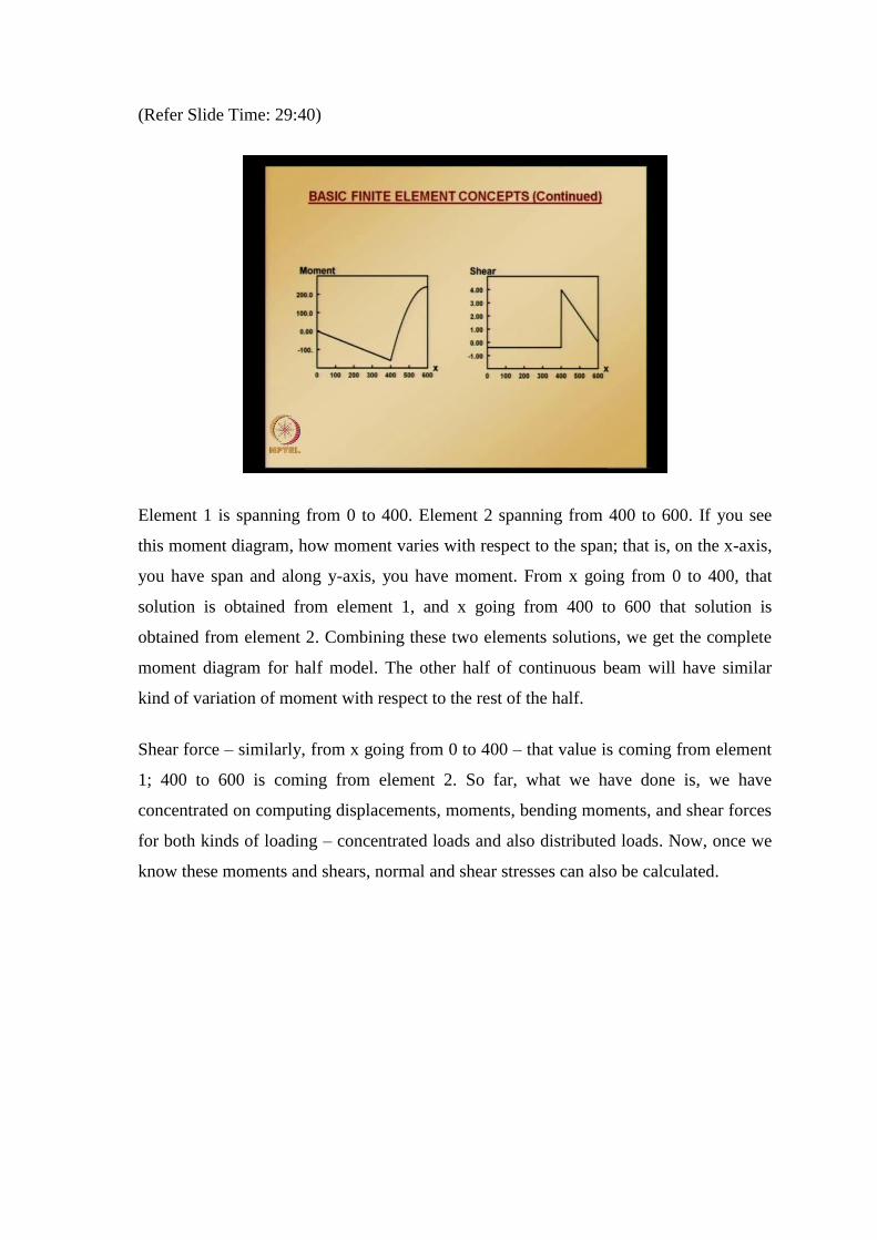
Element 1 is spanning from 0 to 400. Element 2 spanning from 400 to 600. If you see
this moment diagram, how moment varies with respect to the span; that is, on the x-axis,
you have span and along y-axis, you have moment. From x going from 0 to 400, that
solution is obtained from element 1, and x going from 400 to 600 that solution is
obtained from element 2. Combining these two elements solutions, we get the complete
moment diagram for half model. The other half of continuous beam will have similar
kind of variation of moment with respect to the rest of the half.
Shear force – similarly, from x going from 0 to 400 – that value is coming from element
1; 400 to 600 is coming from element 2. So far, what we have done is, we have
concentrated on computing displacements, moments, bending moments, and shear forces
for both kinds of loading – concentrated loads and also distributed loads. Now, once we
know these moments and shears, normal and shear stresses can also be calculated.

(Refer Slide Time: 31:42)
Now, let us see how to calculate stresses in beams – calculation of a normal and shear
stresses. Normal stress at a beam cross section is related to curvature by the equation
given here. Please note that we already derived this equation, when we were deriving
governing equations for beam bending problem, using the assumptions of small
deformation, and also, using the assumption that plane sections remain plane after
bending. We obtained the displacement along the length of the beam value in terms of
transverse displacement; u is equal to minus of y times second derivative of transverse
displacement with respect to x – we obtained that.
Using small deformation assumptions, we got from that displacement u – we got strain.
Using Hooke’s law, we related strain to stress through this material property, Young’s
modulus. That is how we got this equation – normal stress at beam cross section is
related to the curvature by – sigma x is equal to minus E times; E is Young’s modulus; Y
is the distance from the neutral axis to the location where you want to find calculate the
stress. Now, we also know that the relationship between bending moment and curvature;
M is equal to E I times second derivative of transverse displacement with respect to x.
So, we can relate this stress to (Refer Slide Time: 34:01) bending moment. Using
moment curvature equation, we get sigma x is equal to minus of M times y divided by I;
I is second moment of inertia or moment of inertia of cross section. So, whether it is
concentrated load or distributed load, using finite elements, we have seen how to
calculate bending moments at any location in the beam. Once we get bending moment at
any location in the beam, we can use this equation and get the normal stress.
Now, let us look at shear stress computation. Computation of shear stress is more
complicated and depends on shape of cross section. Shear stress can be computed or
calculated by considering a free body diagram of infinitesimal segment of beam along its
length direction, and equating unbalanced normal forces to shear force.
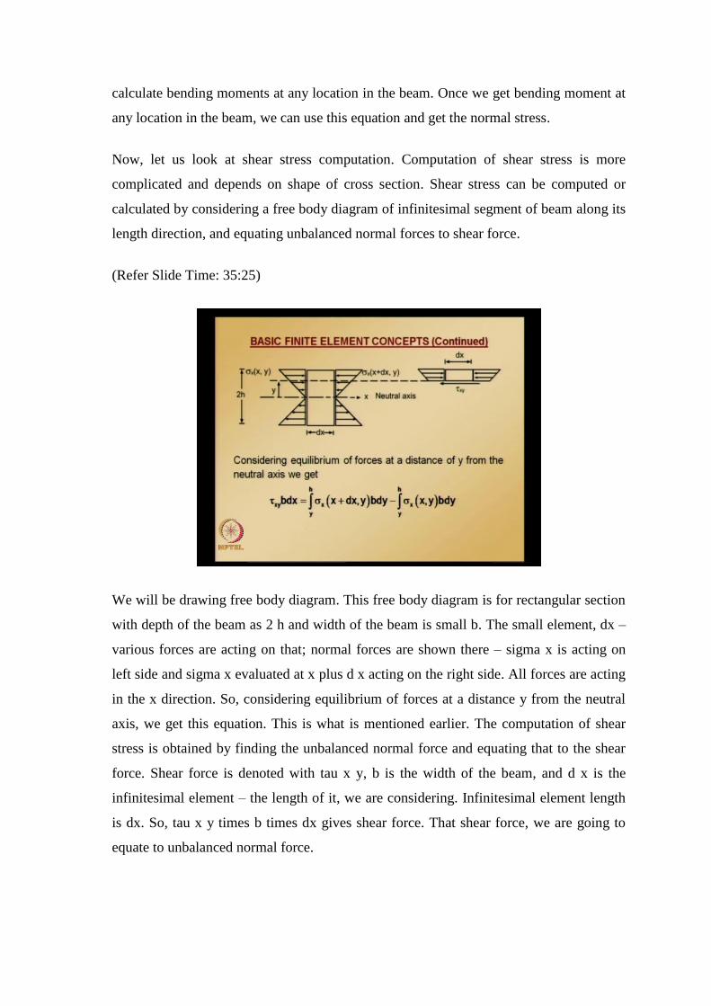
(Refer Slide Time: 35:25)
We will be drawing free body diagram. This free body diagram is for rectangular section
with depth of the beam as 2 h and width of the beam is small b. The small element, dx –
various forces are acting on that; normal forces are shown there – sigma x is acting on
left side and sigma x evaluated at x plus d x acting on the right side. All forces are acting
in the x direction. So, considering equilibrium of forces at a distance y from the neutral
axis, we get this equation. This is what is mentioned earlier. The computation of shear
stress is obtained by finding the unbalanced normal force and equating that to the shear
force. Shear force is denoted with tau x y, b is the width of the beam, and d x is the
infinitesimal element – the length of it, we are considering. Infinitesimal element length
is dx. So, tau x y times b times dx gives shear force. That shear force, we are going to
equate to unbalanced normal force.

Normal force is obtained by multiplying sigma x with b and dy. dy is small slice taken at
a distance y from the neutral axis; thickness of small slice taken at a distance y from the
neutral axis. So, sigma x times width times dy, integrated from 2 h. You note down here
– 2 h is total depth of the beam and neutral axis is coinciding with x-axis. So, the beam
depth goes from h to minus h. So, integrating this sigma x times width times dy from y to
h, gives us normal force. Integrating on either side of this infinitesimal element, we get
what is shown there in that equation on the right-hand side. Simplifying this equation by
substituting what is sigma x; sigma x, we have seen; sigma x is M y divided by I, with a
negative sign.
(Refer Slide Time: 39:02)
Substituting what is sigma x evaluated at x and sigma x evaluated at x plus d x. Also,
here the relationship between moment and shear is also used. We know that derivative of
bending moment gives a shear force. So, that is, substituted that value; dM by dx is
substituted as capital V. Now, we got what is sigma x evaluated at x, sigma x evaluated
at x plus dx. Now, we can substitute these things into the equilibrium equation. We have
written by considering forces acting at a distance y from the neutral axis.

(Refer Slide Time: 39:57)
Here, capital M and capital V are bending moment and shear force acting at the cross
section. Substituting these into equilibrium equation, we get this one – by simplifying.
The stresses for other cross sections can be computed by following similar procedure.
So, we learnt how to calculate normal stress, shear stress. Normal stress is dependent on
bending moment at any point along the length of the beam. Shear stress is dependent on
shear force at any point along the length of the beam. So, once we calculate bending
moment and shear force using finite elements, we can calculate normal stress and shear
stress using these expressions.
Now, we will consider the case of thermal stresses in beams. So far, we have considered
only the mechanical loads; that is, distributed loads and point loads. Now, we will be
seeing how to handle the thermal stresses because of variation of temperatures.

(Refer Slide Time: 42:02)
Consider a beam element subjected to a temperature change that varies linearly
throughout its depth – means you have one temperature at the top surface and another
temperature at the bottom surface. In this kind of situation, the element will experience
curvature, because there is a temperature change between bottom surface and top
surface. This element is going to experience curvature. Curvature is given by this. Here,
the element is shown. Suppose if this beam element is restrained, to undergo this
deformation, fixed-end moments will be developed.
(Refer Slide Time: 43:09)
Curvature, which this element experiences is given by this, which depends on the
temperature change at the top surface of the beam, temperature change at the bottom
surface of the beam, also, coefficient of thermal expansion, and also, depth of the beam.
Here, please do not get confused this h with 2 h earlier. This h is total depth; whereas,
earlier, when we were deriving for the equations for stresses, shear stresses we used – 2 h
to denote the depth of the beam. Here, we used only h. So, this is what I just mentioned.
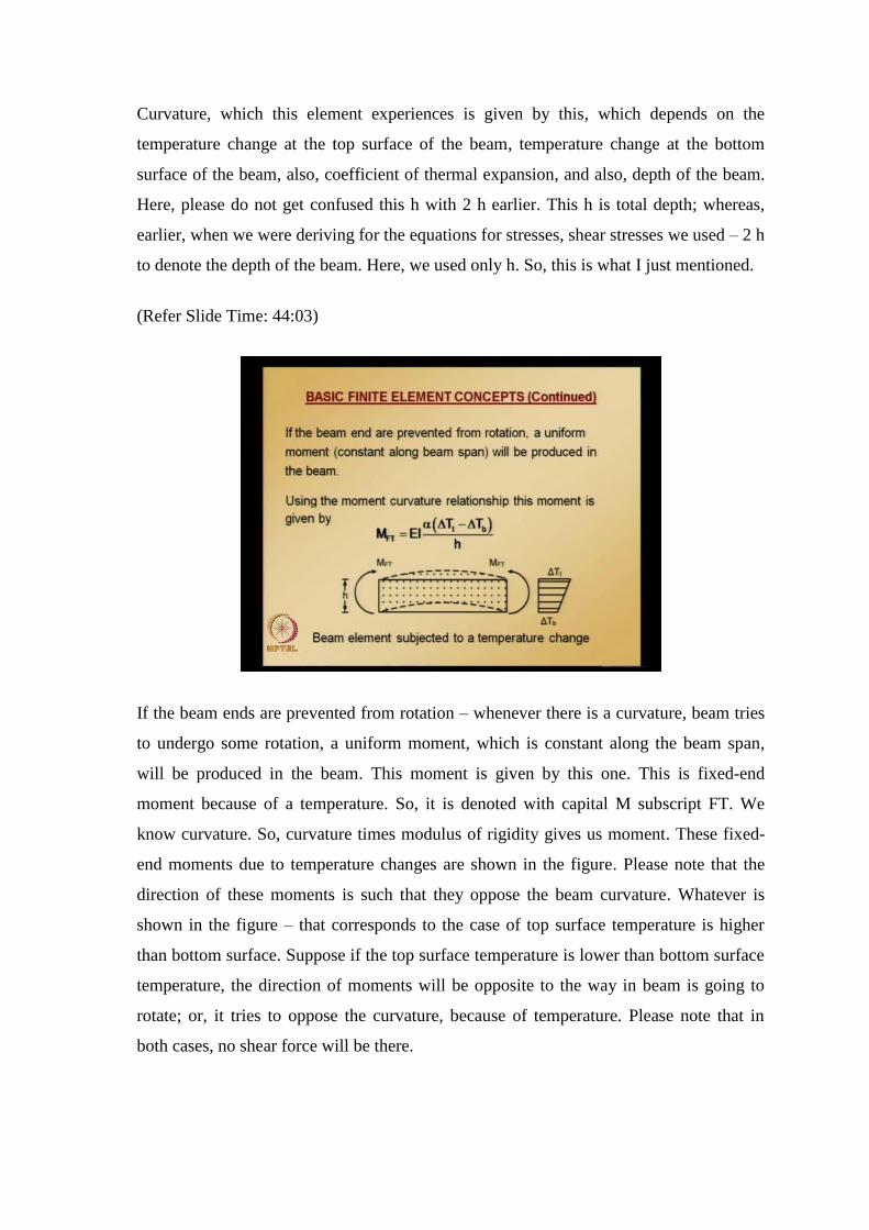
(Refer Slide Time: 44:03)
If the beam ends are prevented from rotation – whenever there is a curvature, beam tries
to undergo some rotation, a uniform moment, which is constant along the beam span,
will be produced in the beam. This moment is given by this one. This is fixed-end
moment because of a temperature. So, it is denoted with capital M subscript FT. We
know curvature. So, curvature times modulus of rigidity gives us moment. These fixed-
end moments due to temperature changes are shown in the figure. Please note that the
direction of these moments is such that they oppose the beam curvature. Whatever is
shown in the figure – that corresponds to the case of top surface temperature is higher
than bottom surface. Suppose if the top surface temperature is lower than bottom surface
temperature, the direction of moments will be opposite to the way in beam is going to
rotate; or, it tries to oppose the curvature, because of temperature. Please note that in
both cases, no shear force will be there.

(Refer Slide Time: 46:09)
With fixed-end moments, remaining analysis is very similar to the distributed load.
Equivalent nodal load vector is equal and opposite to the fixed-end forces and moments.
These point I just mentioned now. Please note that these direction of moments is always
in such a direction to oppose the beam curvature. Whether the temperature of top surface
is higher or lower, in both cases, no shear stresses will be produced.
(Refer Slide Time: 47:13)
Now, we know fixed-end moments. Please note that equivalent nodal load vector – we
have seen this when I am explaining to you the physical interpretation of equivalent
nodal load vector. I mentioned there – equivalent nodal vector is equal and opposite to
the fixed-end forces and moments. So, there are no shear forces; only moments are there
– fixed-end moments.
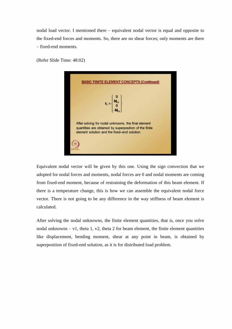
(Refer Slide Time: 48:02)
Equivalent nodal vector will be given by this one. Using the sign convection that we
adopted for nodal forces and moments, nodal forces are 0 and nodal moments are coming
from fixed-end moment, because of restraining the deformation of this beam element. If
there is a temperature change, this is how we can assemble the equivalent nodal force
vector. There is not going to be any difference in the way stiffness of beam element is
calculated.
After solving the nodal unknowns, the finite element quantities, that is, once you solve
nodal unknowns – v1, theta 1, v2, theta 2 for beam element, the finite element quantities
like displacement, bending moment, shear at any point in beam, is obtained by
superposition of fixed-end solution, as it is for distributed load problem.
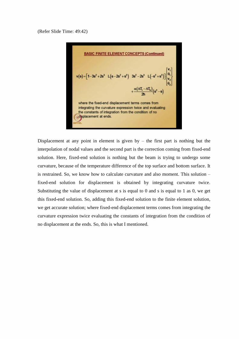
(Refer Slide Time: 49:42)
Displacement at any point in element is given by – the first part is nothing but the
interpolation of nodal values and the second part is the correction coming from fixed-end
solution. Here, fixed-end solution is nothing but the beam is trying to undergo some
curvature, because of the temperature difference of the top surface and bottom surface. It
is restrained. So, we know how to calculate curvature and also moment. This solution –
fixed-end solution for displacement is obtained by integrating curvature twice.
Substituting the value of displacement at s is equal to 0 and s is equal to 1 as 0, we get
this fixed-end solution. So, adding this fixed-end solution to the finite element solution,
we get accurate solution; where fixed-end displacement terms comes from integrating the
curvature expression twice evaluating the constants of integration from the condition of
no displacement at the ends. So, this is what I mentioned.

(Refer Slide Time: 51:15)
Bending moment at any point in the element; as usual, solution obtained by finite
element by interpolating, using finite element shape functions – to that, fixed-end
moment solution is added. Shear force at any point is given by this one. Here, the fixed-
end correction is not appearing, because if you see the curvature expression, the
curvature expression is independent of s. So, when you take one more time derivative of
curvature, it is going to be 0. So, there is no correction for shear force, because of this
temperature or thermal stresses.
We will look an example involving how to calculate the forces, moments in a beam
subjected to thermal stresses, in the next class.