Finite Element Analysis Prof. Dr. B. N. Rao Department …nptel.ac.in/reviewed_pdfs/105106051/lec10.pdfFinite Element Analysis Prof. Dr. B. N. Rao Department of Civil Engineering Indian

Finite Element Analysis

Prof. Dr. B. N. Rao

Department of Civil Engineering

Indian Institute of Technology, Madras

Module - 01

Lecture - 10

(Refer Slide Time: 00:36)

In the last class, we have derived the governing differential equation for beam bending

problem, and we also derived the finite element shear functions, and also we got finite

element equations for beam element, subjected to distributed load like this, having two

nodes x, at x 1 and x 2, and having 2 degrees of freedom at each node v 1 theta 1 at x 1, v

2 theta 2 at x 2. For this, we derived the element equations, which consists of distributed

load, and also point forces, which include forces and moments at node 1 and at node 2.


So, now, in today’s class what will be doing is, we will be using this, whatever we

derived this equation and try to solve some problem. So, now, let us start a problem and

before doing that let me tell you, once we get v 1 theta 1, v 2 theta 2 by solving this

equation system, we can do post processing, that is, we can find displacement at any

point along the beam length, and we derived these equations v as a function of s, where s

goes from 0 to 1, s is equal to 0 corresponds to x 1, and s is equal to 1 corresponds to x 2.

So, once we get v 1 theta 1, v 2 theta 2 we can find displacement at any point along the

beam length by substituting the s value or sweeping s from 0 to 1, we can get the

displacement at any point along the beam length. And similarly, moment can be obtained

using this equation; we already know, that moment is nothing but EI times second

derivative of transverse displacement.

So, taking derivative of previous equation - displacement equation - twice with respect x

and multiplying with EI we get this and we can find the value of moment at any point

along the beam length by varying s from 0 to 1. So, we can sweep from s going from 0 to

1 and get moment at any point along the beam length. Similarly, shear - shear at any

point along the beam length - we can obtain using this equation EI times third derivative

of transverse displacement. So, taking transverse displacement derivative three types and

multiplying with modulus of rigidity EI, we get this equation.

So, you can see from this equation bending moment is linear and shear force is constant

over an element. From mechanics of deformable bodies, we know that exact solution of a

uniform beam, subjected to concentrated loads involve, constant shear and linear bending

moment. Thus the two node element that we just derived, gives exact solution when it is

used to analyze prismatic beams, that is, where EI is constant, subjected to concentrated

loads.

And the exact solution for beam, subjected to uniformly distributed loads can be

obtained by using what is called superposition technique, which will be seeing in a

while. Therefore, analysis of continuous beams in which cross sectional properties do not

change in span requires nodes only at the supports and under the concentrated loads;

whereas non-uniform beams for which EI is not constant throughout the length of the

beam requires more elements per span for better accuracy. So, these things we need to

keep in mind, when we are solving problems related to beam bending using finite

element method.


So, now, we are ready to solve an example. Let us take a simple example, find the

deflection moments and shears in continuous beam shown in figure below, material

properties and geometrical properties of the section of the beam are given. These are

three span continuous beams and each span is of length 400 millimeters and in the

central span 8 kilo Newton point load is applied at the center of the mid-span.

And here, at this problem what we can do is, please note that in finite element method, to

reduce the computational burden, wherever it is possible will be taking symmetry of the

structure or symmetry of the body that we are solving or symmetry of the problem that

we are solving into advantage.


So, here, if you see this three span continuous beam, it is symmetric about the midpoint;

so using symmetry, only half of the beam can be modeled. Taking symmetry into

account, the given problem can be solved using half model like this, and here this soft

model is discretized using two elements - element 1 having degrees of freedom of v 1

theta 1 v 2 theta 2; element 2 having degrees of freedom v 2 theta 2, v 3 and theta 3.

And the load of 8 kilo Newton for the full model since we are considering only half of

the beam that is half, so 4 kilo Newton is applied. And please look at, how symmetry is

taken into account by introducing the support, which is having or which allows vertical

displacement, but rotations are not allowed at the point, where 4 kilo Newton is applied.


So, now, using these boundary conditions and this half model and the load applied of 4

kilo Newton, we can assemble the element equations for element 1. These are the

material properties and geometrical properties and plugging all these things into the

element equations that we derived earlier, we get this. And if you see, there are no loads

applied in the first span or element 1, there are no loads applied; so, all the force vector,

all the components are 0. And for element 2, and also please note that the direction is

positive; if load is applied upward it is positive and if it is applied in the downward

direction it is negative.

So, taking these material properties and geometrical properties element equations for

element 2 are these. Here, directly global degrees of freedom are substituted v 2 theta 2,

v 3 theta 3, and 4 kilo Newton load is applied in the downward direction at node 3, so

minus 4 and please note that all the quantities here, are in kilo Newton and millimeters.

And element 1 is connecting nodes 1 and 2, element 2 is connecting nodes 2 and 3. So, in

the final global equation system, element 1 contribution goes into 1, 2, 3, 4 rows and

columns, and element 2 contribution rows into 3, 4, 5, 6 rows and columns, because at

each node you have 2 degrees of freedom, transfers displacement and rotation.


So, using this information, we can assemble the element equation, we get global

equations. So, here, element 1 contribution, whatever element equations we derived,

element 1 equations contribution went into 1, 2, 3, 4 rows and columns, and element 2

contribution is gone into the rows 3, 4, 5, 6 rows and columns. And here, if you see the

problem, half model v 1 is 0, v 2 is 0 and theta 3 is 0, because rotations are not allowed

at the point, where symmetry is there.


So, the boundary conditions are v 1, v 2 are 0, and also because of symmetry theta 3 is 0.

So, applying these conditions, using these known displacements that is v 1, v 2 theta 3

and theta 3 and introducing unknown reactions, wherever, the displacement boundary

contributions are 0 here, when I say displacement boundary conditions, I mean both

transverse displacement and rotation, wherever displacement boundary conditions are 0,

at the corresponding locations in the force vector, the reactions will be there.

So, using these known displacements and introducing unknown reactions in the right

hand side, we get this equation system. And now, to solve the unknowns, that is, theta 1,

theta 2 and v 3 what we need to do is, we can eliminate the rows and columns

corresponding to the degrees of freedom, whose value is 0. So, three unknown

displacements and rotations can be obtained from the second, fourth and fifth equations.


So, we can eliminate 1, 3 and 6 rows and columns and get the reduced equation system.

So, solving this equations system - reduced equation system - we get theta 1, theta 2 and

vertical or transverse displacements at node 3. The solution of this equation system gives

us these values; please note that rotations are in radians.

And now, we got the solution for this entire half model that is complete solution, that is

we know what is v 1, v 1 is equal to 0, theta 1 is just calculated. Similarly, v 2 is equal to

0, theta 2 is just calculated, and v 3 we calculated and theta 3 is 0.

So, the complete solution for each element can be obtained by substituting the nodal

values, into the trial solution and calculations of displacement bending moment and shear

force for each of the elements are given here for element 1.


Element length and the nodal solution that is v 1 theta 1, v 2 theta 2 and the

displacement, once we got the nodal solution, we can find displacement at any point

along the element length using this equation.


So, in this equation you substitute what is v 1 theta 1, v 2 theta 2 and by sweeping s from

0 to 1, we get the displacement values at any point along the length of the element 1.


Similarly, bending moment can be obtained by using the nodal values in this manner and

now, by substituting s is equal to 0, we get what is the value of moment at the left hand.

By substituting s is equal to 1, we get what is the value of moment at node 2 or at the

second node of element 1. And similarly, shear force - using the nodal values of element

1 that is v 1 theta 1, v 2 theta 2 shear force can be calculated in this manner and please

note that shear force is constant over the entire element length 1.


Similarly, we can repeat the process for element 2. Element 2 length and the nodal

solution that is v 2 theta 2, v 3 theta 3 are given here and using this displacement at any

point along the length of the second element can be obtained by substituting these values

and this equation gives you displacement that is transverse displacement at any point

along length of element 2.


And similarly, bending moment - substituting the nodal values corresponding to element

2, we get bending moment. And again substituting s is equal to 0 we get what is the

value of moment at as at the left end of element 2, and by substituting the value s is equal

to 1, we will get what is the moment value at the right end of element 2.


And now, shear force is again constant over entire length of element 2. And now, please

note that, whatever shear and bending moment that we calculated, they are all internal

shear and internal moment values. So, whenever we try to draw this or put this in a form

of plot, we need to follow sign conventions corresponding to the internal moment and

internal shear that we already started out with.

Now, plotting the values of displacement along the entire half model, that is

displacement over element 1 and displacement over element 2, we get the displacement

variation or how displacement varies over the length or the entire half model length.

Similarly, we got an expression for bending moment and shear force. So, substituting the

values s is equal to 0, s is equal to 1 or s is equal to some other value, we get the bending

moment and shear force at any point along element 1 length and element 2 length.


So, using these we can plot. So, the plot of displacement moment and shear looks like

this. And if you are concerned, whether this, the values that you computed are correct or

not, there is always a check for verifying the results and to do that it is instructive to

draw free body diagrams using bending moment and shear at element ends.


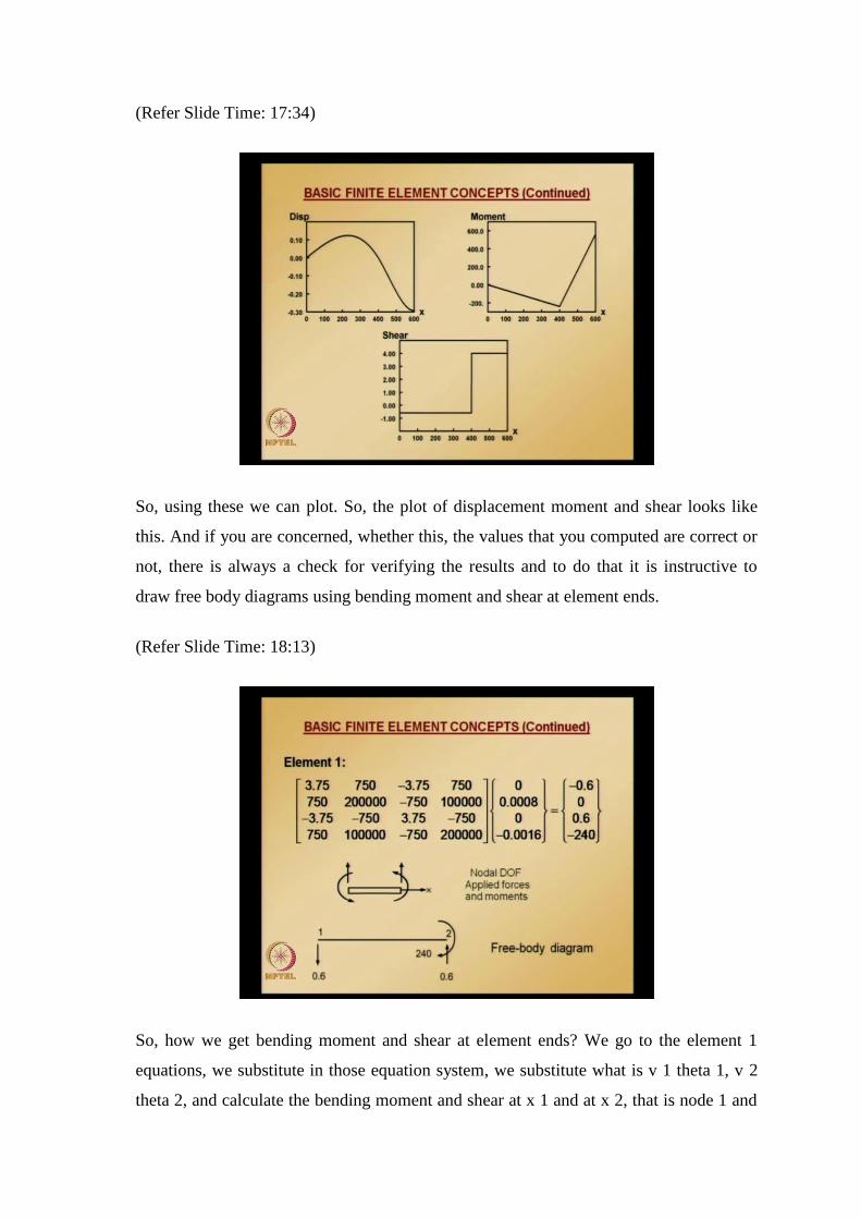
So, how we get bending moment and shear at element ends? We go to the element 1

equations, we substitute in those equation system, we substitute what is v 1 theta 1, v 2

theta 2, and calculate the bending moment and shear at x 1 and at x 2, that is node 1 and

node 2 of element 1. And following the sign conventions and whatever we calculated on

the right hand side, whatever we calculated they are all applied or they are equivalent to

the applied forces and moments.

So, we need to follow sign conventions corresponding to those. So, when you plot this or

when you show these values of minus 0.6, 0, 0.6 minus 240 on a free body diagram for

element 1, it looks like this. Following the sign conventions of a nodal degrees of

freedom and applied forces and moments that we assumed, while we started out with this

beam bending problems.


Similarly, for element 2, substituting the values of v 2 theta 2, v 3 theta 3, we get what

are the bending moment and shear forces at the ends of element 2 and after doing this

calculation it turns out that this values are given there 4, 240, minus 4, 560.

So, if somebody is interested in drawing free body diagram of element 2 taking these

values and following the sign conventions for applied forces and moments and nodal

degrees of freedom, we can draw free body diagram of element 2.

So, now, what we have done is, we have solved this problem using half model and we

got the nodal values. And using the nodal values we computed displacement at any point

along the length of the beam element of both elements 1 and 2, and also moment and

shear and whether the values that we obtained are correct or not we can check using the

free body diagrams. So, what we did is, we have drawn free body diagram of element 1

and free body diagram of element 2.


So, let me put these two figures side by side, free body diagram of element 1 and free

body diagram of element 2 and this is how they look. The support reactions are equal to

sum of shears from elements framing into that support, we know that. So, thus the

reaction at the left support is, at the left support we have only 1 shear that is 0.6 kilo

Newton in the downward direction, and at the middle support, which is contribution is

coming from element 1 and element 2; 0.6 acting in the upward direction, 0.4 acting in

the upward direction; so, total will be 4.6 kilo Newton. So, the reaction at the middle

support is 4.6 kilo Newton upwards; so sum of these two reactions that is 0.6 kilo

Newton acting in the downward direction at the extreme left end, and at extreme left

support and at the middle support reaction of 4.6 kilo Newton. If you had these two

values acting in the upward direction, we get 4 kilo Newton acting in the upward

direction.

So, the overall equilibrium is satisfied, because some of the reactions is equal to and

opposite to the applied forces, applied force is 4 kilo Newton. So, 4 kilo Newton is acting

in the downward direction; some of these reactions of 4 kilo Newton is acting in the

upward direction.

So, overall equilibrium is satisfied. Each element as a free body is also an equilibrium

you can check that some of the forces in the vertical directions are equal to 0 and also

some of are moment taken about any point along each element is 0.

So, also moment at each node are completely balanced, we can see moment at node 2 of

element 1, and moment at node 1 of element 2 they are in the opposite direction, they

balanced each other. So, thus the solution whatever we calculated satisfies all the

equilibrium conditions exactly. Since, the governing differential equation represents

equilibrium condition, this is an indication that we have obtained an exact solution.

Solution obtained from a non-uniform beam generally will not satisfy these equilibrium

checks; the quality of solution. So, the quality of the solution are the error that is

associated with the solution that we obtained using finite element method can be

assessed by performing equilibrium check based on free body diagrams.


So, and taking these two free body diagrams and put them together and this is how

moment and shear looks and that is what we already obtained. And now, let us look at

exact solution of uniform beam subjected to distributed loads, because I mentioned

earlier, that the element equations that we developed gives exact solution for a prismatic

beams and concentrated loadings.

And whereas, to apply those element equations for non-prismatic beams that is beams in

which EI is not constant, EI is varying over along the element length or beam subjected

to distributed loads, it may not be accurate and there will be some error in the solution.


So, the 2 node beam element that we developed is based on cubic trial solution and it

gives exact solution for prismatic beam subjected to concentrated loads however, when

beam is subjected to distributed loads, the standard finite element solution gives nodal

displacements, that is the displacements and rotations at the nodes are going to be exact,

but moments and shears are not very good.

So, to demonstrate this behavior, consider a finite element analysis of simply supported

beam that is shown here, which is subjected to uniform distributed load. The exact

solution for this problem is well known and it is available in elementary mechanics of

material books.

And the exact solution for this problem is transverse displacement at the left end is 0 and

at mid-span the transverse displacement is 5 over 384 qL power 4 over EI, q is a

distributed load. And rotation at the left end is qL cube over 24 EI and at the mid-span it

is 0; bending moment at the left end is 0 and at the mid-span is minus qL square over 8,

and shear force minus qL over 2 at the left end and 0 at the mid-span.

So, we know the exact solution for this problem. Now, let see how, if I apply finite

element method using two elements, how the solution looks or what is the accuracy of

solution that we get for this problem using two finite elements.


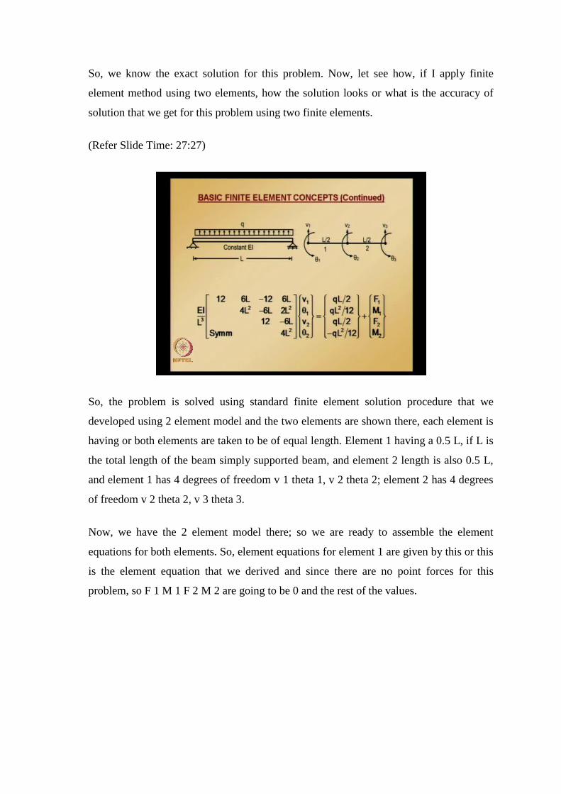
So, the problem is solved using standard finite element solution procedure that we

developed using 2 element model and the two elements are shown there, each element is

having or both elements are taken to be of equal length. Element 1 having a 0.5 L, if L is

the total length of the beam simply supported beam, and element 2 length is also 0.5 L,

and element 1 has 4 degrees of freedom v 1 theta 1, v 2 theta 2; element 2 has 4 degrees

of freedom v 2 theta 2, v 3 theta 3.

Now, we have the 2 element model there; so we are ready to assemble the element

equations for both elements. So, element equations for element 1 are given by this or this

is the element equation that we derived and since there are no point forces for this

problem, so F 1 M 1 F 2 M 2 are going to be 0 and the rest of the values.


Here, a length of each element is 0.5 L; so in the element equations that are shown there,

L needs to be replaced with 0.5 L and by doing that we get element equations for

element 1 to be these in which L is equal to 0.5L is substituted and also since both

elements are identical and the length of both elements are 0.5, so the element equations

for element 1 and element 2 are same and that is given by this equation. Now, we got

element equations for element 1, element 2; so now, we are ready to assemble global

equations. And there are three nodes at each node; we have 2 degrees of freedom and

element 1 contribution goes into 1, 2, 3, 4 rows and columns, element 2 contribution

goes into 3, 4, 5, 6 rows and columns of the global equations.



So, that is simplified form of each element equation. Assembling equations of two

elements, global equations are obtained as follows. And now, for the 2 element model

that we have taken, node 1 is at the left support and node 3 is at the right support. So, v 1

and v 3 are going to be 0, because we have supports at node 1 and node 3.


So, substituting essential boundary conditions, essential boundary conditions are v 1 is

equal to 0, v 3 is equal to 0. Introducing known reactions, introducing unknown reactions

corresponding to these known displacements; so, wherever essential boundary conditions

are 0, reactions will be developed at those locations in the force vector and the global

equations are as follows. And to solve this equation system what we can do is, we can

eliminate the rows and columns corresponding to the degrees of freedom for which

whose value is 0.


So, we get reduced equation system and which we can solve for theta 1 v 2 theta 2 and

theta 3 and if you solve, this is the reduced equation system and if you solve this

equation system using any of the symbolic computations or the software which can do

symbolic computations, if you can solve this equation system, we get solution for theta 1

v 2 theta 2 v 3.

Please note that, node 2 corresponds to the mid-span of this simply supported beam and

note that finite element, mid-span displacement and rotations are same as the exact

solution of the problem.


So, using these nodal values - bending moments and shears can be calculated for element

1 and element 2. And also you can see these values that we calculated that is, theta 1 v 2

theta 2 and theta 3 all match exactly with the exact solution which is already shown to

you.

So, now, let us try to calculate what is the bending moment and shear in element 1 and

element 2, using this nodal values. So, moment at any point along element 1 is given by

this equation by sweeping s from 0 to 1.

Similarly, shear at any point along element 1 is given by this equation, which is shear is

constant, it is constant everywhere at any point along the element 1 length or it is

constant and value is equal to minus qL over 4; it is not a function of s.

And from this shear at s is equal to 0, we have seen earlier what is the exact value of

shear at the left end and what is the bending moment value at the mid-span. So, to get the

shear at the left end, substitute s is equal to 0 and to get bending moment, the mid-span,

substitute s is equal to 1.


So, from this equation the shear at the left end, that is, s is equal to 0 and moment at mid-

span at s is equal to 1 or these values. And the exact values exact end shear force and

mid-span bending moment are these values.

So, you can see the values that we obtained using 2 element model using the finite

element formulation or finite element equation that we developed, when we apply to this

simply supported beam subjected to distributed load, there is an error and this error is

quite large and this happened only in shear force and bending moment.

And even though the displacement that is displacements, I mean rotations and transverse

displacements, even though they are exact, shear and moment are not good at all. The

standard finite element approach to improve these calculations of moments and shear is

to use large number of finite elements for span, wherever a distributed load is there on

that particular span. And the results will be closer to the exact solution if more elements

are used, and but there is a better way of handling the situation to get exact solution with

just 1 element for span.

The main idea in this approach is to treat the problem as a superposition of two separate

problems. So, we will see what is that superposition method. Now, because the solution

that we got using 1 element solution for 2 element solution for simply supported beam

subject to distributed load, even though the displacements are accurate, moments and

shears are not accurate.

So, one solution is, you can use large number of elements, but that is not smart way of

solving the problem; the other solution is superposition technique. So, we will be looking

into it now.


So, let us assume, the first figure shows the actual problem and regardless of actual

supports in the first problem, the element ends are assumed to be fixed against any

displacement or rotation such as structure will experience moments and shears in the

loaded span alone and that is, each loaded span is independent, fixed end beam. Exact

solutions for these fixed end beam problems are easily available in elementary

mechanics of material books.

For example, so, now, the actual problem which is shown in the first figure what will be

doing is, irrespective of whatever boundary conditions we have for each span, we will

assume each of this span to be fixed and when we say each span is fixed, each span is

going to be independent and whatever is happening in the other span is not going to

affect any span. So, and in each particular span the moments and shears we can get from

the fixed end solution that are already documented in most of the mechanics of material

books.


So, now, for example, if we take a fixed end beam subjected to uniform upward load, the

displacement, bending moment and shear at any point along the span are given by these

formulas, where s goes from 0 to 1, s is equal to 0 corresponds to the left end; s is equal

to 1 corresponds to the right end.


So, at any point along the beam length by changing the s value, we can get what is the

transverse displacement value, moment and shear. So, the actual problem is irrespective

of the boundary conditions what we will do is, we will assume each span to be fixed and

we get this fixed end moments, which I just showed you for fixed end, one span fixed

end beam subjected to uniform upward displacement load I showed you displacement,

bending moment and shear this equation solutions. So, similar kind of solutions we can

obtain for many standard or elementary mechanics of material books. And so, using

those values you can find what is the fixed end moments and the shear in each of the

spans.

And the second problem is, the actual support conditions are used, which is shown in

third figure, actual support conditions are used at the element ends; concentrated forces

and moments that are equal and opposite to those obtained from fixed end beam

solutions that we obtained for the fixed end conditions are applied the nodes. This

structure that is which is shown in third figure is analyzed using finite element method

since only concentrated forces are applied, finite element solution yields exact solution.

And sum of the two solutions, that is the figure shown in a and b, sum of these two

solutions corresponds to the solution of the original problem that is actual problem,

which is shown in the first figure. Thus the final element forces and moments are

obtained by superposition of both the solution from fixed end beam solution and the

concentrated load finite element solution.

And let see how this effects, how this super position effects the computation of element

solution and actually it effects only after calculating the nodal values obtained in the

usual manner; even though the superposition method is two-step process for

understanding purposes it is actually going to affect only in the final computation of the

element solutions after obtaining the nodal values, which we can obtain as in the usual

manner.

So, what we will do is, what we can do is we can proceed in the usual manner of writing

elements equations, assembling them and solving from for the nodal unknowns, when

computing element quantities the exact solution of the fixed end problem is added to the

finite element solution.


So, for example, for the case of uniformly distributed load using exact fixed end solution

what we can do is, these are the exact fixed end beam solutions that is for transverse

displacement, moment and shear.


And if you want to solve a beam, which is subjected to distributed load what you can do

is, you can solve as usual using finite element method and get the nodal values. When

you are calculating moments and shears what you can do is, you can add to the solution

that you get for using moment and shears finite elements, the fixed end solution.

So, for displacement at the nodal values, whatever you get from finite element method

that is exact, but any at any point in between we need to add the fixed end moment

solutions.


So, the correction factor is shown, whatever is shown the second term is a correction

factor, which is coming from fixed end solution. And bending moment at any point, once

we get the nodal values as usual we can calculate bending moment at any point along the

beam length and to that we add fixed ends solution.


Please note that here, this fixed end solution corresponds to uniformly distributed load

and if you have some other load, then we need to add fixed end solution corresponding to

that particular load. And shear, we need to add the correction factor, which is the second

term in this equation.

So, with this, we can find the exact solution for not only displacements at the nodes, but

also displacement at any point along the beam length, and also moments and shears

along the beam length, even if you use 1 element solution by this superposition method.

And we will look into an example, instead of taking even two elements that we did

earlier, we can even use 1 element, if we are using the superposition method and we will

see how using this correction of the fixed end solution, how we obtain the exact solution.

Documents

Finite Element Analysis Prof. Dr. B. N. Rao Department …nptel.ac.in/reviewed_pdfs/105106051/lec10.pdfFinite Element Analysis Prof. Dr. B. N. Rao Department of Civil Engineering Indian