Embed Size (px)
Citation preview
Linkaru C., Ciucă V., Pîrciog S., Atanasiu D.,Regional Science Inquiry Journal, Vol. V, (1), 2013, pp. 43 -73 43
FINDING UNDERLYING FACTORS USING THE INDEPENDENT COMPONENT ANALYSIS ON LABOUR MARKET – APPLICATION ON
UNEMPLOYMENT RATE IN MONTHLY VARIATION
Cristina LINKARU
National Institute for Science Research in The Field of Labour and Social Protection- INCSMPS, Romania, e-mail: [email protected]
Vasilica CIUCĂ
National Institute for Science Research in The Field of Labour and Social Protection- INCSMPS,
Romania, e-mail: [email protected]
Speranţa PÎRCIOG
National Institute for Science Research in The Field of Labour and Social Protection- INCSMPS, Romania, email: [email protected]
Draga ATANASIU
National Institute for Science Research in The Field of Labour and Social Protection- INCSMPS, Romania, email: [email protected]
Abstract
Independent Component Analysis ICA is “a method for finding underlying factors or components from multivariate (multidimensional) statistical data”. Considering that the specific of this method is “that it looks for components that are both statistically independent and Non-Gaussian, we try to apply ICA method on labour market data. Following the methodology presented by Hyvärinen, Karhunen, Oja (2001) on the problem” cashflow of several stores belonging to the same retail chain, trying to find fundamental factors common to all stores that affect the cash flow” we apply on analysing the unemployment rates, seasonally adjusted, in monthly variation at EU27 level between January 2000-
September 2011. The data source is EUROSTAT, indicator [une_rt_m]: „Unemployment rate, monthly average, seasonally adjusted data, total (%), resulting 141 months/cases. Orginal mixture data are pre-processing in the stage of Pre-whitened using Principal Component Analysis PCA, with NIPALS algorithm and for ICA the FastICA Algorithm from STATISTICA 8.0 Software.
Keywords: unemployment rate, monthly variation, ICA, PCA
JEL classification: J6
„Most measured quantities are actually mixtures of other quantities..”1
1. Introduction
Starting from Hyvärinen, Karhunen, Oja financial applications2 of Independent Component Analysis ICA as “a method for finding underlying factors or components from multivariate
(multidimensional) statistical data”, considering that the specific of this method is “that it looks for components that are both statistically independent and nongaussian, we try to apply ICA method on labour market data.
1 J.V. Stone, (2005): A Brief Introduction to Independent Component Analysis in Encyclopedia of Statistics in Behavioral Science, Volume 2,
pp. 907–912, Editors Brian S. Everitt & David C. Howell, John Wiley & Sons, Ltd, Chichester, 2005 ISBN 978-0-470-86080-9 2 K. Kiviluoto şi E. Oja, Independent component analysis for parallel financial time series. În Proc. ICONIP'98, vol.2, pg. 895-898, Tokio,
Japan, 1998.
44 Linkaru C., Ciucă V., Pîrciog S., Atanasiu D.,Regional Science Inquiry Journal, Vol. V, (1), 2013, pp. 43 -73
Following the methodology presented3 on the problem” cashflow of several stores belonging to the same retail chain, trying to find fundamental factors common to all stores that affect the cash flow” we apply on analysing the unemployment rate, seasonally adjusted, in monthly variation at EU27 level between January 2000-September 2011. The data source is EUROSTAT, indicator [une_rt_m]: „Unemployment rate, monthly average, Seasonally adjusted data, total (%), resulting 141
months/cases. ICA is based on the idea that independence is a stronger property then unecorrelatedness [PCA]. Uncorrelatedness in itself is not enough to separate the components”,”PCA or factor analysis cannot separate the signals: they gave components that are uncorrelated”4 Among the applications of the ICA there are already some on econometrics – parallel time series financial data5. 2. Data treatment as signal from informational perspective
According with the ICA theory the working unit is a signal. If “any signal represents form the mathematical point of view a time function” 6 then we shall point some specific characteristics under this assumption:
On the labour market there are studied behaviours of the individual during the economic activity span. If there are used micro data organised in longitudinal data base we can tell that we
increase the chances to model better the reality. When reference is to the individual the variables could be compared with “analogical signals”: the individual lives as continuous function with emitted continuous values in R7
:
:
f
f
(1)
Data treatment as signal from informational perspective allow the conversion analogue in digital or the conversion from continuum in discreet8 through precise procedures that combines operations like: discretization, sampling, quantification, coding, etc. In the technical literature those operations could be described as functions of time (see Fig. 1)
Signals transmits amplitudes and „any signal could be decompose in sum of the sinusoidal
signals –subject of the Fourier Analysis”9.
Sinusoidal signals are orthogonal and are the only ones from nature able to propagate through linear systems without to be distorted (is changing only the amplitude and phase). Sinusoidal signals contains extremely small information:
x(t) = x(A, T, t) (2)
t
Tf
tAtx
*
1
)*sin()(
3 Hyvärinen, Karhunen, Oja, Independent Component Analysis, 2001 John Wiley & Sons, pg.441.
4 Hyvärinen, Karhunen, Oja, Independent Component Analysis, 2001 John Wiley & Sons, pg.7.
5Kiviluoto K. and E. Oja. Independent component analysis for parallel financial time series. In Proc. ICONIP'98, volume 2, pages 895-898,
Tokyo, Japan, 1998. 6 Ioan P. Mihu, Despre semnale şi sisteme din volumul Procesarea numerică a Semnalelor, pg.2
7 Laurenţiu Frangu – Introducere în Inginerie Electronică şi Telecomunicaţii, 2008, pg. 30
8 Laurenţiu Frangu – Introducere în Inginerie Electronică şi Telecomunicaţii, 2008
9 William Stallings, Data and computer communications, Chapter 3, transmisia datelor,
http://ftp.utcluj.ro/pub/users/cemil/prc/Chapt_3ro.ppt#256,1,William Stallings Data and Computer Communications
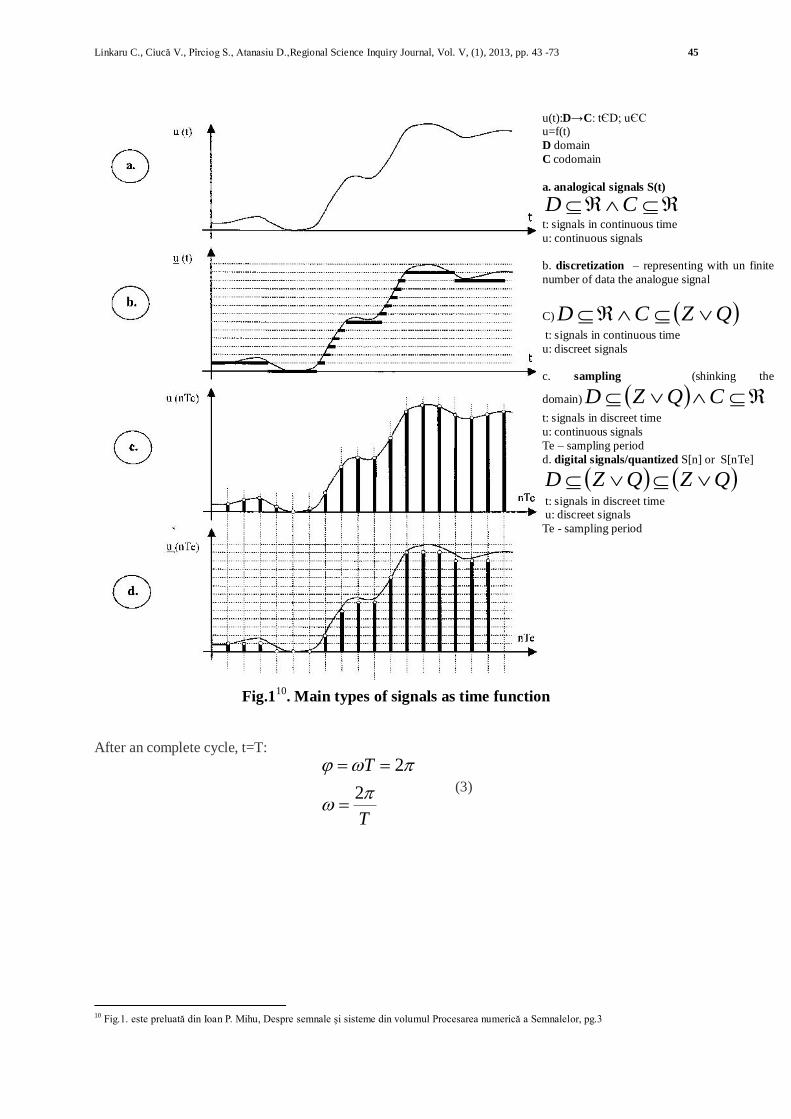
Linkaru C., Ciucă V., Pîrciog S., Atanasiu D.,Regional Science Inquiry Journal, Vol. V, (1), 2013, pp. 43 -73 45
Fig.1
10. Main types of signals as time function
After an complete cycle, t=T:
T
T
2
2
(3)
10
Fig.1. este preluată din Ioan P. Mihu, Despre semnale şi sisteme din volumul Procesarea numerică a Semnalelor, pg.3
u(t):D→C: tЄD; uЄC u=f(t)
D domain
C codomain
a. analogical signals S(t)
CD
t: signals in continuous time
u: continuous signals
b. discretization – representing with un finite
number of data the analogue signal
C) QZCD
t: signals in continuous time
u: discreet signals
c. sampling (shinking the
domain) CQZD
t: signals in discreet time
u: continuous signals
Te – sampling period
d. digital signals/quantized S[n] or S[nTe]
QZQZD
t: signals in discreet time u: discreet signals
Te - sampling period
46 Linkaru C., Ciucă V., Pîrciog S., Atanasiu D.,Regional Science Inquiry Journal, Vol. V, (1), 2013, pp. 43 -73
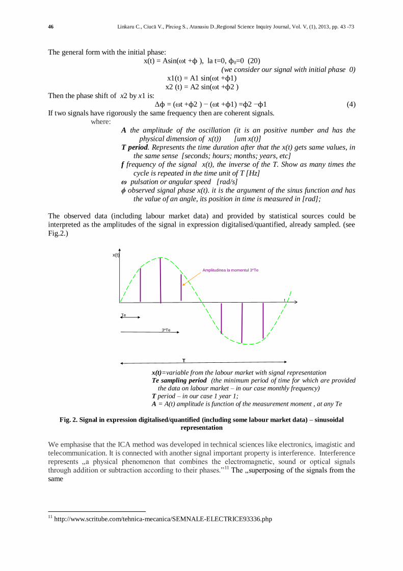
The general form with the initial phase: x(t) = Asin(ωt +ϕ ), la t=0, ϕ0=0 (20)
(we consider our signal with initial phase 0) x1(t) = A1 sin(ωt +ϕ1)
x2 (t) = A2 sin(ωt +ϕ2 )
Then the phase shift of x2 by x1 is: Δϕ = (ωt +ϕ2 ) − (ωt +ϕ1) =ϕ2 −ϕ1 (4)
If two signals have rigorously the same frequency then are coherent signals. where:
A the amplitude of the oscillation (it is an positive number and has the physical dimension of x(t)) [um x(t)]
T period. Represents the time duration after that the x(t) gets same values, in the same sense [seconds; hours; months; years, etc]
f frequency of the signal x(t), the inverse of the T. Show as many times the
cycle is repeated in the time unit of T [Hz] ω pulsation or angular speed [rad/s] ϕ observed signal phase x(t). it is the argument of the sinus function and has
the value of an angle, its position in time is measured in [rad]; The observed data (including labour market data) and provided by statistical sources could be interpreted as the amplitudes of the signal in expression digitalised/quantified, already sampled. (see
Fig.2.)
x(t)
Amplitudinea la momentul 3*Te
t
Te
3*Te
T
x(t)=variable from the labour market with signal representation
Te sampling period (the minimum period of time for which are provided
the data on labour market – in our case monthly frequency)
T period – in our case 1 year 1;
A = A(t) amplitude is function of the measurement moment , at any Te
Fig. 2. Signal in expression digitalised/quantified (including some labour market data) – sinusoidal
representation
We emphasise that the ICA method was developed in technical sciences like electronics, imagistic and telecommunication. It is connected with another signal important property is interference. Interference represents „a physical phenomenon that combines the electromagnetic, sound or optical signals through addition or subtraction according to their phases.”11 The „superposing of the signals from the same
11
http://www.scritube.com/tehnica-mecanica/SEMNALE-ELECTRICE93336.php
Linkaru C., Ciucă V., Pîrciog S., Atanasiu D.,Regional Science Inquiry Journal, Vol. V, (1), 2013, pp. 43 -73 47
frequency band (difference between maximum and minim of the frequency’s , fmax-fmin =LBs) 12. This mixing phenomenon of the signals could distort the original signal. “Under certain conditions, the signals underlying measured quantities can be recovered by making use of ICA. ICA is a member of a class of blind source separation (BSS) methods.”13
3. Method Independent Component Analyis ICA
The modelling and prediction of the dynamics of the macroeconomic factors using the Independent Component Analyis – ICA is still at beginning. Hyvärinen, Karhunen and Oja14 affiliate this method among the methods „for finding underlying factors or components from multivariate (multidimensional) statistical data”. This method is strongly differentiated from others through the two essential hypotheses that are simultaneously realised: the component looked for are both independent
(one component doesn’t offer any information about the other component) in statistical sense and is non-Gaussian (have not a normal distribution). This method allows the linear representation only based on multivariate signals/data offering a „learned” representation without supervisor, as neuronal calculus type. The intrinsic data message exploration includes the ICA method under the data mining and exploratory data analysis methods. First mention of this method was signalled in 1980, by J. Herault, C. Jutten, B. Ans15, in neuronal signal processing data. The next step in this method development was represented signal separation of sources solutions (including BSS blind sources
separation) by J.F. Cardoso, P. Comon16, J.L.Lacoume, A. Cichocki and R. Unbehauen. The exponential growth of the computers power brings in attention of the users from different fields those techniques developed in more „strict technical fields” [brains imagistic, imagines processing, signal deconvolution, telecommunications – lately other signals from mobile communication CDMA (Code-Division Multiple Access), etc.]. The Fast Independent Component Analysis (FICA) or FastICA algoritm (created by Hyvärinen, Karhunen, Oja) enhanced the popularity of the method ICA because of its efficiency and new applications like: Hopfield networks, self organised maps Kohonen SOM, JADE algorithm, Cichocki-Unbehauen algorithm, etc. FastICA could be applied now on different
software environments (MATLAB 5 /5.2., C++/C, STATISTICA 8.0, as well as dedicated soft). The STATISTICA 8.0. environment offer two options: the simultaneous extraction variant (parallel) and the successive extraction variant (one unit at the time- artificial neuron with the weight of an vector, neuron under the property of being able to learn – named also deflation). We highlight the expanding tendency of ICA’s borrowing in economics17. The financial domain registered the first applications of those techniques especially on parallel data similar with the econometric applications in parallel time series separations, decomposing in independent component which offers a new perspective over the
data structure. In view to apply those techniques are respected the independence hypothesis and non-Gaussianity of the components/factors that describes in a linear representations the measured multivariate data.
12
Iacob, Sisteme şi tehnici multimedia, http://andrei.clubcisco.ro/cursuri/5master/tagcmrv-stm/01_stmm1_intro.ppt#273,33,Slide 33 13
Stone, J.V. (2005): A Brief Introduction to Independent Component Analysis in Encyclopedia of Statistics in Behavioral Science, Volume 2,
pp. 907–912, Editors Brian S. Everitt & David C. Howell, John Wiley & Sons, Ltd, Chichester, 2005 ISBN 978-0-470-86080-9 14
Hyvärinen, Karhunen, Oja, Independent Component Analysis, 2001 John Wiley & Sons, pg.1. 15
Cited from „Martin Sewell, Independent Component Analysis, Department of Computer Science University College London
http://www.stats.org.uk/ica/: „ANS, B., J. H´ERAULT, and C. JUTTEN, 1985. Adaptive neural architectures: Detection of primitives. In:
Proceedings of COGNITIVA’85. pp. 593–597. // H´ERAULT, J., and B. ANS, 1984. Circuits neuronaux ´a synapses modifiables:
D´ecodage de messages composites par apprentissage non supervis´e. Comptes Rendus de l’Acad´emie des Sciences, 299(III-13), 525–528.
// H´ERAULT, J., C. JUTTEN, and B. ANS, 1985. D´etection de Grandeurs Primitives dans un Message Composite par une Architecture de
Calcul Neuromim ´etique en Apprentissage non Supervis´e. In: Actes du X`eme colloque GRETSI. pp. 1017–1022.” 16
COMON, Pierre, 1994. Independent Component Analysis, A New Concept?, Signal Processing, 36(3), 287–314. 17
K. Kiviluoto şi E. Oja, Independent component analysis for parallel financial time series. În Proc. ICONIP'98, vol.2, pg. 895-898, Tokio, Japan, 1998.
48 Linkaru C., Ciucă V., Pîrciog S., Atanasiu D.,Regional Science Inquiry Journal, Vol. V, (1), 2013, pp. 43 -73
Box 118
18
Hyvärinen Aapo and Erkki Oja, Independent Component Analysis: Algorithms and Applications Neural Networks Research Centre,
Helsinki University of Technology, pg.2
Independent Component Analysis ICA/ Nongaussian factor analysis “A generative model – it describes how the observed data are generates by a process of mixing the components
sj”[book, ICA, Hyvarinen, Karhunen, Oja,pg.151]
Assumption the components si are statistically independent-
the key to estimating the ICA model is nongaussianity
a gaussian variable has the largest entropy among all random variables of equal
variance. Negentropy is in some sense the optimal estimator of nongaussianity
the independent component must have nongaussian distributions
we observe n linear mixtures x1, ...,xn of n independent components
xj = aj1s1+aj2s2+...+ajnsn, for all j.
xj(t), observed values, mixture xj, random vector
sk(t) independent component (“source” means here an original signal, latent variables, meaning that they cannot be directly observed.), is a random variable, instead of a proper
time signal, nongaussian
The ICA model: x = As,
A mixing matrix
s =Wx=A
-1x
W un-mixing/ separation matrix
ICA consists in estimating both the s(t) and A(t), (j=k)
Ambiguities of ICA 1. We cannot determine the variances (energies) of the independent components
2. We cannot determine the order of the independent components.
Preprocessing for ICA Centering - the observed signals are centred around their means so that the transformed signals have
zero mean Whitening - linearly transforming the observed signals X into a new set of variables, which are
uncorrelated and their variances equal unity
The FastICA Algorithm: algorithm for maximizing the contrast function - nonquadratic function G
Deflation - which extracts one principal component at a time.
Parallel or Multiple Extraction and its multi unit version.
Linkaru C., Ciucă V., Pîrciog S., Atanasiu D.,Regional Science Inquiry Journal, Vol. V, (1), 2013, pp. 43 -73 49
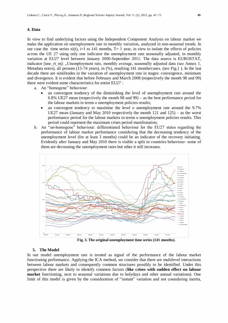
4. Data
In view to find underlying factors using the Independent Component Analysis on labour market we make the application on unemployment rate in monthly variation, analyzed in non-seasonal trends. In our case the time series xi(t), i=1 to 141 months, T= 1 year, in view to isolate the effects of policies
across the UE 27 using only one indicator the unemployment rate seasonally adjusted, in monthly variation at EU27 level between January 2000-September 2011. The data source is EUROSTAT, indicator [une_rt_m]: „Unemployment rate, monthly average, seasonally adjusted data (see Annex 1, Metadata notes), all persons (15-74 years), in (%), resulting 141 months/cases. (see Fig.1 ). In the last decade there are similitudes in the variation of unemployment rate in stages: convergence, minimum and divergence. It is evident that before February and March 2008 (respectively the month 98 and 99) there were evident some characteristics for entire EU27 :
a. An “homogene” behaviour:
an convergent tendency of the diminishing the level of unemployment rate around the 6.8% UE27 mean (respectively the month 98 and 99) – as the best performance period for the labour markets in terms o unemployment policies results;
an convergent tendency to maximise the level o unemployment rate around the 9.7%
UE27 mean (January and May 2010 respectively the month 121 and 125) – as the worst performance period for the labour markets in terms o unemployment policies results. This period could represent the maximum crises period manifestation;
b. An “un-homogene” behaviour: differentiated behaviour for the EU27 states regarding the performance of labour market performance considering that the decreasing tendency of the unemployment level (for at least 3 months) could be an indicator of the recovery initiating. Evidently after January and May 2010 there is visible a split in countries behaviour- some of
them are decreasing the unemployment rates but other it still increases.
0,0
5,0
10,0
15,0
20,0
2000M01 2001M01 2002M01 2003M01 2004M01 2005M01 2006M01 2007M01 2008M01 2009M01 2010M01 2011M01
EU27
Belgium
Bulgaria
CzechRepublic
Denmark
Germany
Estonia
Ireland
Greece
Spain
France
Italy
Cyprus
Latvia
Lithuania
Luxembourg
Hungary
Malta
Netherlands
Austria
Poland
Portugal
Romania
Slovenia
Slovakia
Finland
Sweden
United Kingdom
Fig. 3. The original unemployment time series (141 months).
5. The Model
In our model unemployment rate is treated as signal of the performance of the labour market functioning performance. Applying the ICA method, we consider that there are multilevel interactions between labour markets and consequently common structures possibly to be identified. Under this perspective there are likely to identify common factors (like crises with sudden effect on labour
market functioning, next to seasonal variations due to holydays and other annual variations). One limit of this model is given by the consideration of “instant” variation and not considering inertia,
50 Linkaru C., Ciucă V., Pîrciog S., Atanasiu D.,Regional Science Inquiry Journal, Vol. V, (1), 2013, pp. 43 -73
delays, etc. Based on the perspective that the interdependency between the European economies is increasing, and then the unemployment rates at national level are not “pure” but mixed signals using this method could be an high potential to surprise also the effect of labour market policies of every country (passive and active measures). In this context we try to apply ICA method in view to isolate
the new clusters generated under the actions of “European” underlying factors, grouped by a common
“behaviour”.
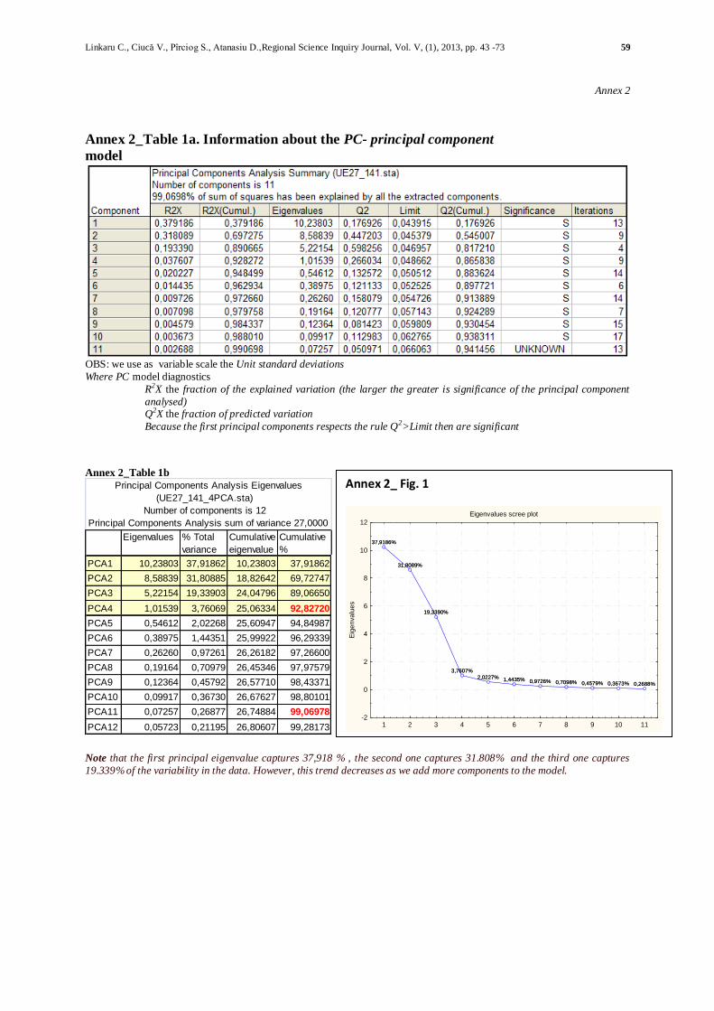
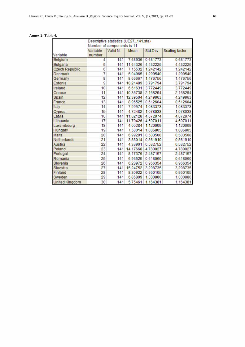
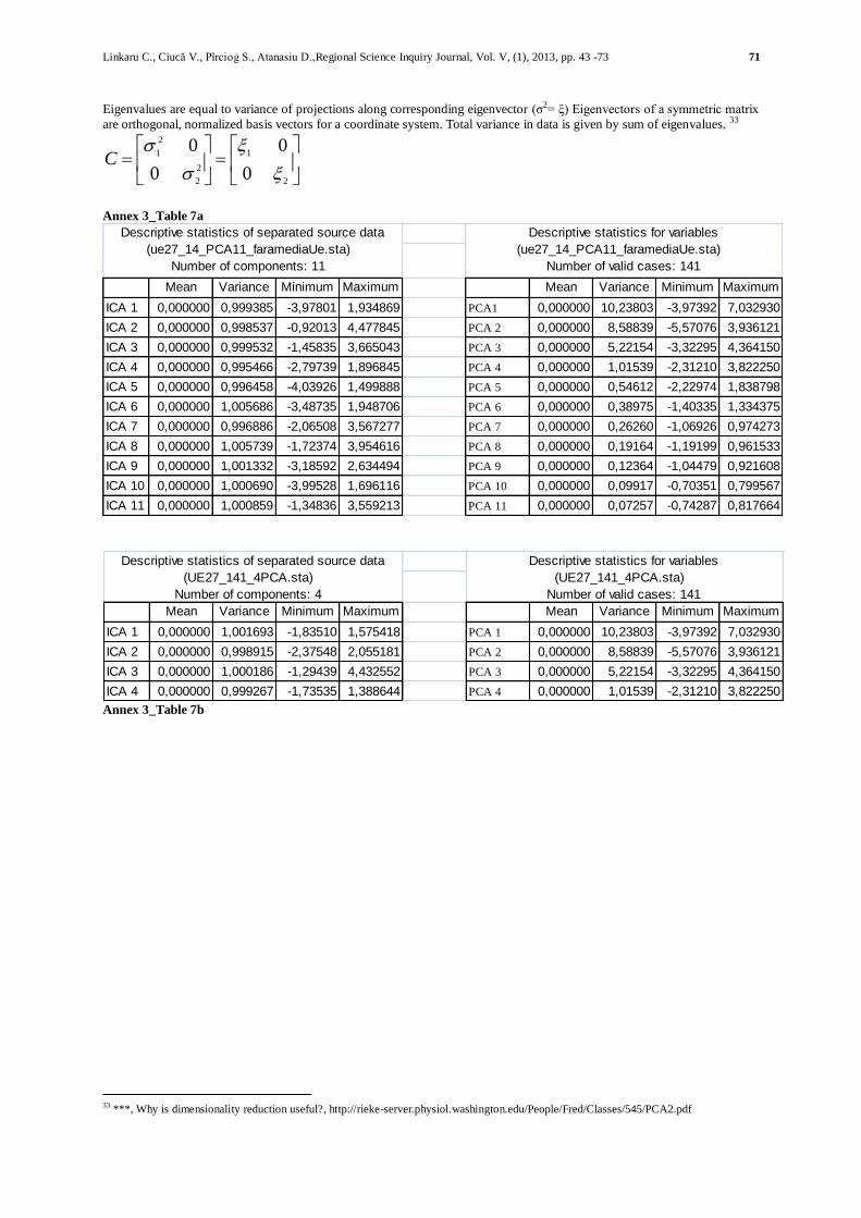
5a. Pre-whitened data using PCA
The original 27 dimensional signal was projected to the subspace spanned by 11 principal components (covering 99,0697% from total variance of Eigenvalues, see Annex 2_Table 1a and b, Fig.1). The level of the Eigenvalue indicate also the importance (rank) of the principal component, PCA 1
captures 37,918 % , the PC 2 captures 31.808%, PC 3 captures 19.339%, etc. of the variability in the data. Choosing the number of principal components could be a problem. If we apply a threshold of minim 90% variance of the Eigenvalues then the minimum PCA components will be 4 that cover 92.8272% from total variance of it. So, from the original space of 27 dimension we reduce to an interval of 4 to 11 variables with less redundancy, that conserves as good as possible the initial characteristics.” In PCA the redundancy is measured by correlations between data elements, while in ICA the much richer concept of independence is used, and in ICA the reduction of the number of
variables is given less emphasis. Using only the correlation as in PCA has the advantage that the analysis can be based on second-order statistics only, In connection with ICA, PCA is a useful pre-processing step…(for ICA first step) data can be pre-processed by whitening, removing the effect of first and second order statistics”19. Using the STATISTICA 8.0 software we apply PCA as multivariate exploratory technique under variants offered by „STATISTICA PLS20 with the state-of-the art NIPALS algorithm for building PLS models (Geladi and Kowalski, 1986). The algorithm assumes that the X and Y data have been transformed to have means of zero. This procedure starts with an initial guess value for the t-scores u
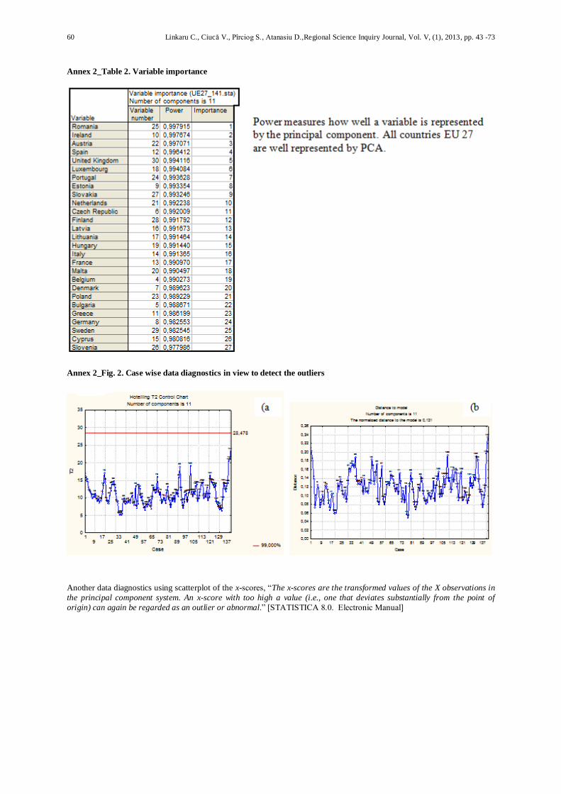
and iteratively calculating the model properties in separate and subsequent steps”. Applying NIPALS algorithm with Maximum number of iteration: 50, Convergence criterion=0.0001, Fitting method =Number of components by cross validation V-fold (V value 7), resulted 11 components, noted PCA 1 to PCA 11. The variable importance as a measure o the maximum power of component representation is offered by the model with 11 PCA (see annex 2_Table 2). In Annex 2_ Fig. 2 a and b there are presented the case wise data diagnostics in view to detect the
outliers through: “Hotelling T2 Control Chart” and “Distance to Model Chart”. The outlier’s analysis
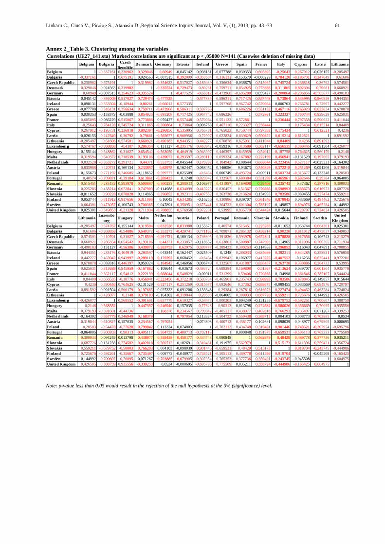
reflects that for the last decade there become visible an abnormal tendency in unemployment, localised in the last intervals 140-141 months, corresponding for the months August-September 2011, the end of our series. As a measure of increasing interdependency between the European economies is the growing tendency of clustering among variables unemployment rates for the EU27. In Annex 2_Table 3 is presented with red the significant correlation coefficients between the selected variables. There are relations (positive or negative) one to many, for each country. Austria, Belgium, Netherland and Poland
indicate greater independence (over 8/26 insignificant coefficients). On the other extreme Czech Republic, Hungary, Denmark, Italy, Lithuania, Malta, Slovenia indicate labour market sensitiveness (only 3/26 insignificant coefficients). As particular case Romania indicates positive dependency
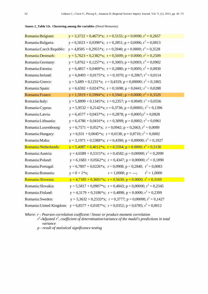
with all countries UE26. As a detail, Romania’s highest dependency of the unemployment variation is with France - explains 35,5% from original variability and indicates through the regression coefficient 0.599% as monthly medium increase, as a measure of the "proportional" to each other are two variables.
19
Hyvärinen A., Karhunen, Oja, Independent Component Analysis, 2001 John Wiley & Sons, Chapter 6. Principal Component analysis and
whitening, pg. 125 20
Partial Least Squares (PLS) (also known as Projection to Latent Structure) is a popular method for modelling industrial applications. It
was developed by Wold in the 1960s as an economic technique, but soon its usefulness was recognized by many areas of science and
applications including Multivariate Statistical Process Control (MSPC) in general and chemical engineering in particular.
Linkaru C., Ciucă V., Pîrciog S., Atanasiu D.,Regional Science Inquiry Journal, Vol. V, (1), 2013, pp. 43 -73 51
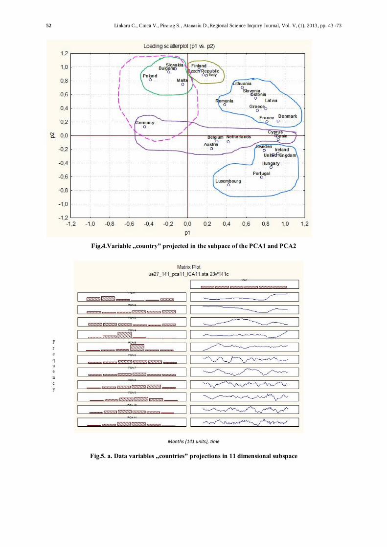
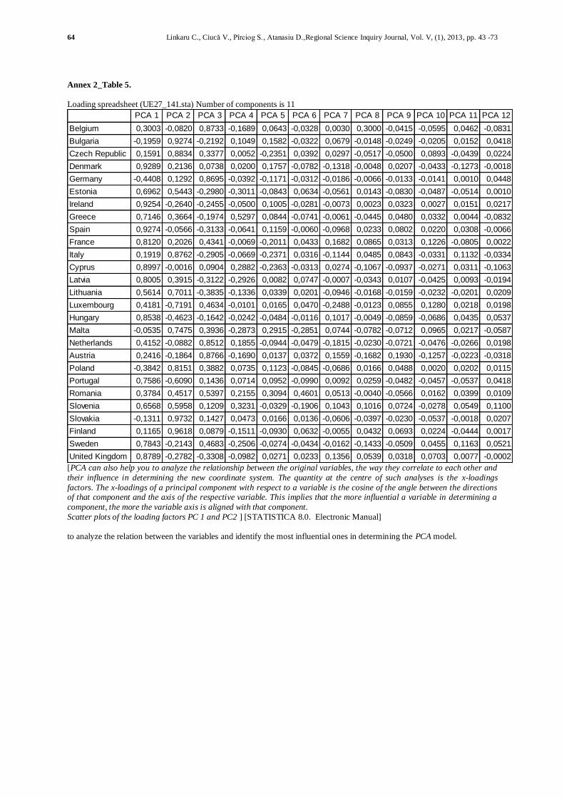
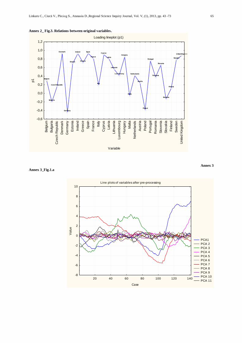
Relations between original variables could be described also in the new coordinate system resulted through PCA applying. This system offers also an image regarding the way in which the original variables are correlated to each other and their influence in determining a component. In Annex
2_Table 5 is presented the Correlations of the variable „country” with each factor PCA. Also „variables placed close to each other influence the PCA model in similar ways, which also indicates
they are correlated” 21To illustrate better this is presented in Annex 2_ Fig.3. the line plot (p1) of the variable “country” against the loadings of PC1. In reference with PCA1 Malta is the less influential role and UK plays the most influential role in determining the first PC1. In Fig. 4 we identify some possible clusters, after the projection of every input vector “country” into subspace, with orthogonal factors/component, given by the PCA1 (p1) and PCA2 (p2) – components that capture almost 70% variability in the data. It is possible to delimitate the following clusters:
o Positive correlation with both factors PCA1 and PCA2 is registered for: First group: Lithuania, Slovenia, Estonia, Latvia, Greece, France, Denmark, Romania. Second group (more with the PCA2, uncorrelated with PCA1): Finland, Czech Republic, Italy o Positive correlation with PCA1 and negative correlation with PCA2 Sweden, Ireland, United Kingdom, Hungary, Portugal, Luxemburg o Positive correlation with PCA2 and negative (Germany at this extreme) correlation with PCA1(Malta the other extreme): Poland, Bulgaria, Slovakia.
In Fig.5 a and b there is presented the matrix plot of the data variables „countries” projections in 11 dimensional subspace and 4. Regardless the changing of the number of dimensions the loadings are the same.
5b. Results: Finding underlying factors using the Independent Component Analysis on
labour market – application on Unemployment rate in monthly variation
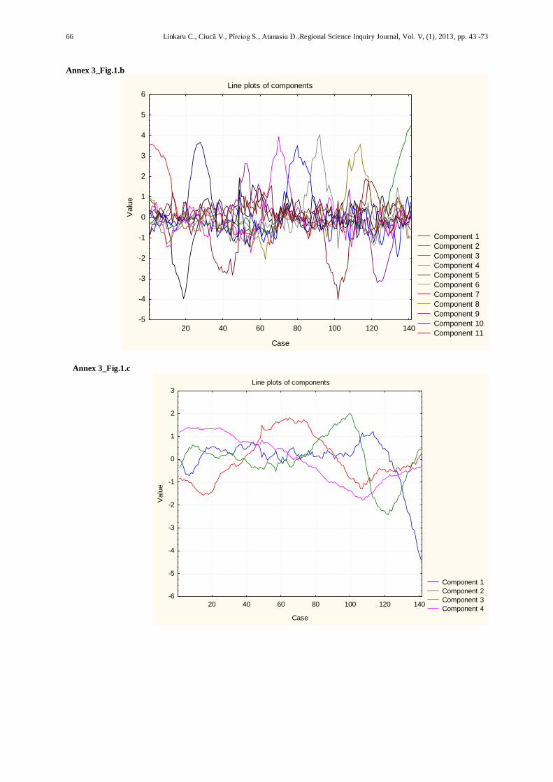
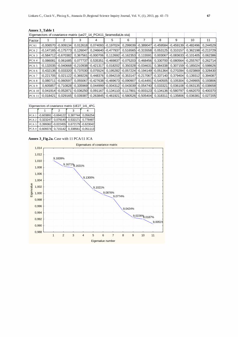
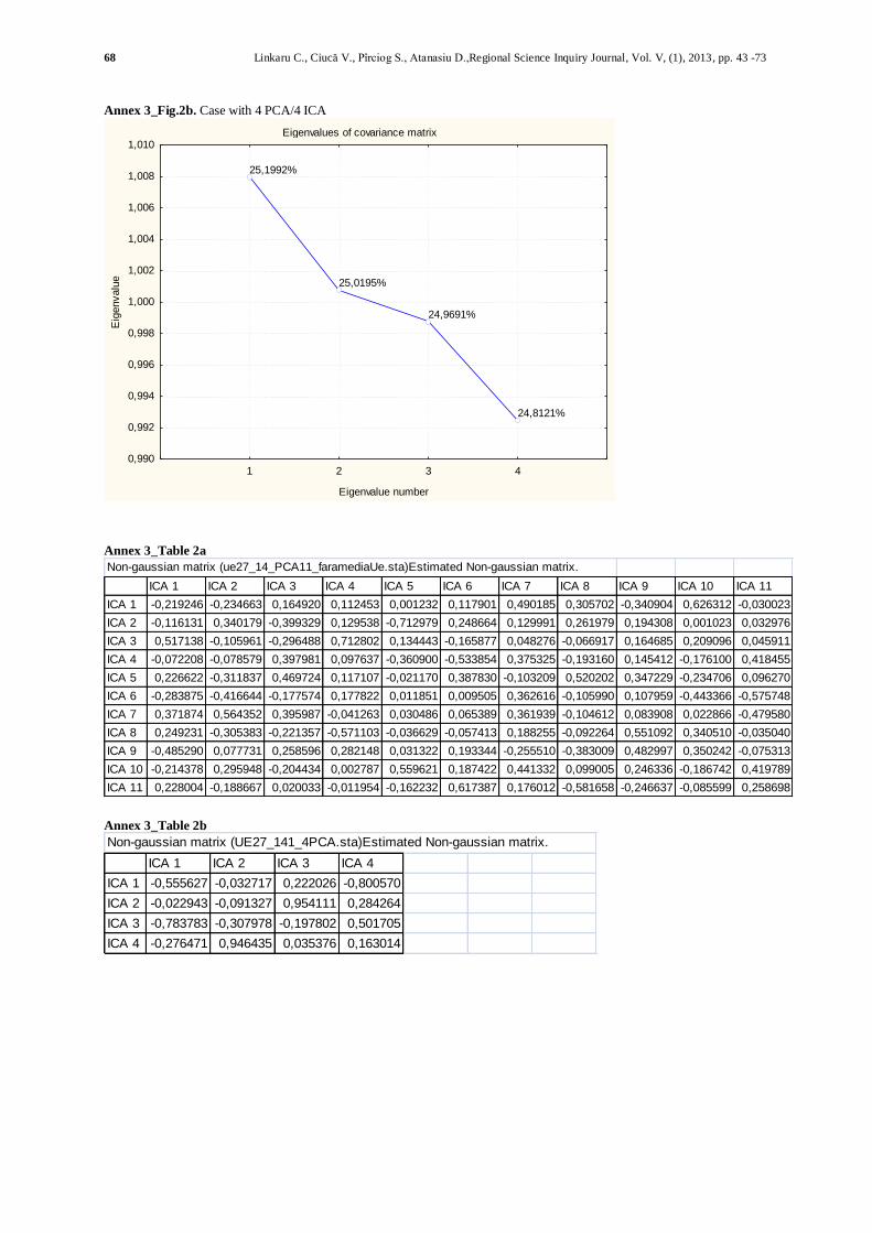
Applying PCA we obtained uncorrelated components noted as PCA 11 (Annex 3 fig.1a.), but not
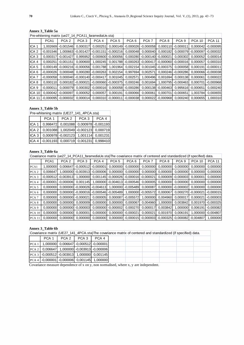
independent. In Annex 3_Table 6a and b is presented that the PCA 11 (and also the variant PCA 4) are uncorrelated with their covariance is 0.” The main reason why we calculate the ICA’s for two dimensions 11 and 4 is sustained but the comment “in real world application is that there is no prior knowledge on the number of independent components. Sometimes the Eigen values spectrum of the data covariance matrix can be used, but in this case the Eigen values decreased ratter smoothly without indicating any clear signal subspace dimension. Then the only way is to try different dimensions. If the independent components that are found using different dimensions for the whitened
data are the same or very similar, we can trust that they are not just artefacts produced by compression, but truly indicate some underlying factors in the data.”22 Another property is that if they are independent then they are uncorrelated but unecorrelatedness doesn’t imply independence. In the literature there are some considerations useful like:
Whiteness, an slightly stronger property then unecorelatedness of zero mean vector means
that its components are uncorrelated and their variance equal unity.- the covariance (as well as
correlation matrix) matrix equals the identity matrix ;23
ICA: factors are called “sources” and learning is “unmixing”. Since latent variables assumed to be independent, trying to find linear transformation of data that recovers independent
causes24
.
21
[STATISTICA 8.0. Electronic Manual] 22
Hyvärinen A., Karhunen, Oja, Independent Component Analysis, 2001 John Wiley & Sons, pg.442 23
Hyvärinen A., Karhunen, Oja, Independent Component Analysis, 2001 John Wiley & Sons, pg.159 24
CSC2515: Lecture 8 Continuous Latent Variables, Lecture 9: Continuous, Latent Variable Models
http://www.cs.toronto.edu/~hinton/csc2515/notes/lec7middle.pdf
52 Linkaru C., Ciucă V., Pîrciog S., Atanasiu D.,Regional Science Inquiry Journal, Vol. V, (1), 2013, pp. 43 -73
Fig.4.Variable „country” projected in the subpace of the PCA1 and PCA2
Months (141 units), time
Fig.5. a. Data variables „countries” projections in 11 dimensional subspace
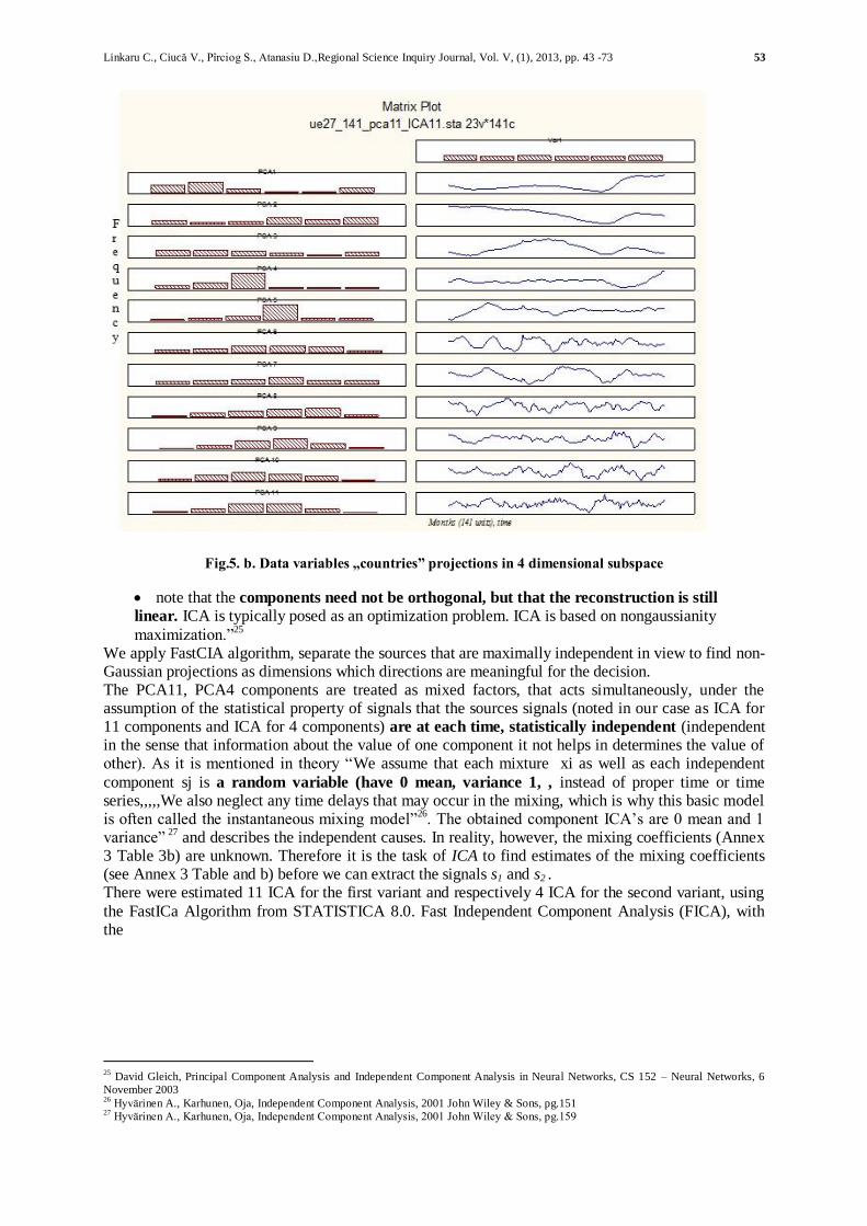
Linkaru C., Ciucă V., Pîrciog S., Atanasiu D.,Regional Science Inquiry Journal, Vol. V, (1), 2013, pp. 43 -73 53
Fig.5. b. Data variables „countries” projections in 4 dimensional subspace
note that the components need not be orthogonal, but that the reconstruction is still
linear. ICA is typically posed as an optimization problem. ICA is based on nongaussianity
maximization.”25 We apply FastCIA algorithm, separate the sources that are maximally independent in view to find non-Gaussian projections as dimensions which directions are meaningful for the decision. The PCA11, PCA4 components are treated as mixed factors, that acts simultaneously, under the assumption of the statistical property of signals that the sources signals (noted in our case as ICA for 11 components and ICA for 4 components) are at each time, statistically independent (independent in the sense that information about the value of one component it not helps in determines the value of other). As it is mentioned in theory “We assume that each mixture xi as well as each independent
component sj is a random variable (have 0 mean, variance 1, , instead of proper time or time series,,,,,We also neglect any time delays that may occur in the mixing, which is why this basic model is often called the instantaneous mixing model”26. The obtained component ICA’s are 0 mean and 1 variance” 27 and describes the independent causes. In reality, however, the mixing coefficients (Annex 3 Table 3b) are unknown. Therefore it is the task of ICA to find estimates of the mixing coefficients (see Annex 3 Table and b) before we can extract the signals s1 and s2 . There were estimated 11 ICA for the first variant and respectively 4 ICA for the second variant, using
the FastICa Algorithm from STATISTICA 8.0. Fast Independent Component Analysis (FICA), with the
25
David Gleich, Principal Component Analysis and Independent Component Analysis in Neural Networks, CS 152 – Neural Networks, 6 November 2003 26
Hyvärinen A., Karhunen, Oja, Independent Component Analysis, 2001 John Wiley & Sons, pg.151 27
Hyvärinen A., Karhunen, Oja, Independent Component Analysis, 2001 John Wiley & Sons, pg.159
54 Linkaru C., Ciucă V., Pîrciog S., Atanasiu D.,Regional Science Inquiry Journal, Vol. V, (1), 2013, pp. 43 -73
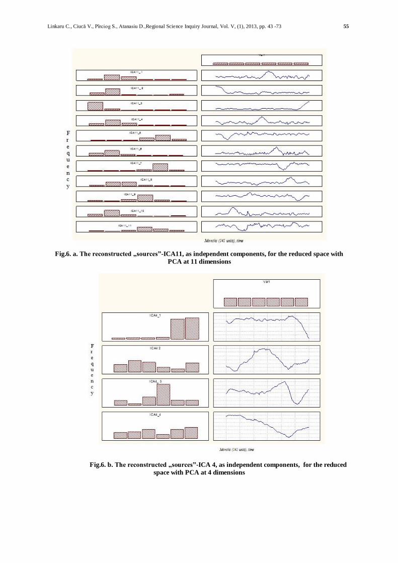
parallel extraction method (The components are extracted simultaneously), Function used in the approximation to neg-entropy Nonquadratic function G: Log-cosh, normalised variables. So the result obtained is calculated for the 2 dimensions 11 and 4, of this endeavour is presented in the Fig. 6 a and b, The reconstructed „sources”- ICA11, as independent components, for the reduced space with PCA at 11 (4) dimensions.
In view to shape better the data model, we keep in mind that it describes a structure “specifies a dedicated grammar for a dedicated artificial language for (a specific) domain, represents classes of entities (kinds of things) ....., (contains) information and the attributes of that information, and relationships among those entities and (often implicit) relationships among those attributes”28. In our analyze trends excludes the seasonal influences and make possible to identify Factors with sudden effect on labour market functioning in general, and over the unemployment variation in particular. Our sources could have different interpretations, like:
ICA11_1: starting point (minimum) august 2005, maximum point august 2006. Visible effects of the Europe transition from EU15 to EU25, following May 2004, 10 more countries joined the EU: the Czech Republic, Estonia, Cyprus, Latvia, Lithuania, Hungary, Malta, Poland, Slovenia and Slovakia29 are New Members of UE, (Hurricane Katrina struck Florida and the Gulf Coast after the August), increasing the unemployment rate in EMU countries, etc,; ICA11_2: starting point (maximum) January 2000 – initiating the Lisbon Strategy; ICA11_3: starting point (minimum) February 2010 – evident effects of the global crises on
increasing the unemployment; ICA11_4: minimum July 2004, maximum October, 2005; …etc …….
At this point there is a lot to work and also interpretations are also possible. Maybe our model is not well stabilised because at the dimension variations, the components found are not virtually the same. Using the found mixing coefficients it is also possible to analyse the original time series and cluster them in groups.
Based on the perspective that the interdependency between the European economies is increasing, and then the unemployment rates at national level are not “pure” but mixed signals using this method could be a high potential to surprise also the effect of labour market policies of every country (passive and active measures).
6. Final remarks
„The ICA success is dependent by the key hypothesis that regards the physical world philosophy
approach. This hypothesis sustain that variables or the independent signals are generates by different physical processes.”30 Stone (2005), with the convention that the term of signal is interchangeable with the term of variable, emphasis independence in the ICA context using the argument that two independent signals do not allow the prediction of one using the other. The empirical experience in the science field (physics, biology, IT, price stocks, etc.) has demonstrated that, without any doubt, in reality most of the measured signals have to be independent signals mixtures. Regardless its limits, “ICA is a very general technique in which are observed random data linear transformed in independent
component, maximum independent one regard the other and in the same time they have “ interesting distributions”, this method allow the optimised estimation of latent variables model”31. The increasing computing capacity brings in the users attention also these techniques imported from strict technical domains. Beyond the analogy of signal theory with the labour market field, it is still a challenge to interpret the results obtained through this method. The idea to better exploit this relatively new technique represents only the frame and impetus to keep learning.
28
http://en.wikipedia.org/wiki/Data_model#Data_structure 29
http://epp.eurostat.ec.europa.eu/statistics_explained/index.php/Glossary:European_Union_(EU) 30
Bell, A.J. & Sejnowski, T.J. (1995). An information maximization approach to blind separation and blind deconvolution, Neural
Computation 7, 1129–1159. 31
http://research.ics.tkk.fi/ica/
Linkaru C., Ciucă V., Pîrciog S., Atanasiu D.,Regional Science Inquiry Journal, Vol. V, (1), 2013, pp. 43 -73 55
Fig.6. a. The reconstructed „sources”-ICA11, as independent components, for the reduced space with
PCA at 11 dimensions
Fig.6. b. The reconstructed „sources”-ICA 4, as independent components, for the reduced
space with PCA at 4 dimensions
56 Linkaru C., Ciucă V., Pîrciog S., Atanasiu D.,Regional Science Inquiry Journal, Vol. V, (1), 2013, pp. 43 -73
Selective Bibliography
Bell A.J. and T.J. Sejnowski. Learning higher-order structure of a natural sound.
Network, 7:261-266, 1996. Bell A.J. and T.J. Sejnowski. The 'independent components' of natural scenes are edge filters. Vision
Research, 37:3327-3338, 1997. Bell, A.J. & Sejnowski, T.J. (1995). An information maximization approach to blind separation and
blind deconvolution, Neural Computation 7, 1129–1159. Buzuloiu A., Sofron E., Institutul National de Cercetare-Dezvoltare în Informatica,Universitatea din
Pitesti ICI, Bucuresti http://www.ici.ro/RRIA/ria2004_3/art02.htm Cardoso, J. (2000). On the stability of source separation algorithms, Journal of VLSI Signal
Processing Systems 26(1/2), 7–14
Catalin Dumitrescu, Universitatea Politehnica Bucuresti, ANALIZELE TIMP-FRECVENTA DIN CLASA COHEN, http://rria.ici.ro/ria2005_2/art04.htmlComon P., Independent Component Analysis - a new concept?, Signal Processing, 36 287-314, 1994.
Creţu Train, Fizică Generală, Editura Tehnică 1984 Didier G. Leibovici and Christian Beckmann, An introduction to Multiway Methods for Multi-Subject
fMRI experiment, FMRIB Technical Report 2001, Oxford Centre for Functional Magnetic Resonance Imaging of the Brain (FMRIB), Department of Clinical Neurology,
University of Oxford, John Radcliffe Hospital, Headley Way, Headington, Oxford, UK. Esbensen K. H., Guyot D., Westad F., Houmøller L. P., Multivariate Data Analysis in Practice,
Aalborg University, third Edition, pp.10, Oslo: Camo Process AS, 2002. Gheorghe Puscasu, Bogdan Codres, Semnale si metode de procesare,
http://facultate.regielive.ro/cursuri/automatica/semnale_si_metode_de_procesare-117361.html
Hurri J., A. Hyvärinen, and E. Oja. Wavelets and natural image statistics. In Proc. Scandinavian Conf. on Image Analysis '97, Lappenranta, Finland, 1997.
Hyvärinen A., (2001). Complexity pursuit: separating interesting components from time series, Neural Computation13, 883–898.
Hyvärinen A., and Erkki Oja, Independent Component Analysis: A Tutorial, node14: Negentropy, Helsinki University of Technology Laboratory of Computer and Information Science;
Hyvärinen A., E. Oja, P. Hoyer, and J. Hurri. Image feature extraction by sparse coding and independent component analysis.In Proc. Int. Conf. on Pattern Recognition (ICPR'98), pages 1268-1273, Brisbane, Australia, 1998.
Hyvärinen A., Karhunen, Oja, Independent Component Analysis, 2001 John Wiley & Sons Hyvärinen A., Survey on Independent Component Analysis , Helsinki University of Technology
Laboratory of Computer and Information Science P.O.Box 5400, FIN-02015 HUT, Finland, [email protected] http://www.cis.hut.fi/~ aapo/, http://cis.legacy.ics.tkk.fi/aapo/papers/NCS99web/
Hyvärinen A., What is Independent Component Analysis, http://www.cs.helsinki.fi/u/ahyvarin/whatisica.shtml
Hyvärinen Aapo and Erkki Oja, Independent Component Analysis: Algorithms and Applications Neural Networks Research Centre, Helsinki University of Technology, pg.11
Hyvärinen, Aapo, Juha Karhunen, Erkki Oja, Independent Component Analysis, A volume in the Wiley Series son adoptive and Learning Systems for Signal Processing, Communications and Control, Simon Haykin, Series Editor, 2001;
Iacob, Sisteme şi tehnici multimedia, http://andrei.clubcisco.ro/cursuri/5master/tagcmrv-stm/01_stmm1_intro.ppt#273,33,Slide 33
Jutten C. and J. Herault., Blind separation of sources, part I: An adaptive algorithm based on
neuromimetic architecture. Signal Processing, 24:1-10, 1991; Karhunen J., A. Hyvärinen, R. Vigario, J. Hurri, and E. Oja. Applications of neural blind separation to
signal and image processing. In Proc. IEEE Int. Conf. on Acoustics, Speech and Signal Processing (ICASSP'97), pages 131-134, Munich, Germany, 1997.
Kiviluoto K. and E. Oja. Independent component analysis for parallel financial time series. In Proc. ICONIP'98, volume 2, pages 895-898, Tokyo, Japan, 1998.
Linkaru C., Ciucă V., Pîrciog S., Atanasiu D.,Regional Science Inquiry Journal, Vol. V, (1), 2013, pp. 43 -73 57
Laurenţiu Frangu – Introducere în Inginerie Electronică şi Telecomunicaţii, 2008, pg.33 Lt. col. ing. Szilagyi A., REZUMATUL TEZEI DE DOCTORAT, TEMA: CONTRIBUŢII LA
REALIZAREA MODELĂRII RECEPTOARELOR DE RĂZBOI ELECTRONIC DE RADIOLOCAŢIE, Conducător de doctorat: Colonel (r) prof. univ. dr. ing. Gheorghe GAVRILOAIA BUCUREŞTI, 2006, pp.57
Makeig, A.J. Bell, T.-P. Jung, and T.-J. Sejnowski. Independent component analysis of electroencephalographic data. In Advances in Neural Information PRocessing S. Systems 8, pages 145-151. MIT Press, 1996.
Nisbet Robert, John Elder, John Fletcher Elder, Gary Miner, Handbook of statistical analysis and data mining applications, 2009, http://books.google.ro/books?id=U5np34a5fmQC&pg=PA168&lpg=PA168&dq=Simultaneous+Extraction+and+Deflation&source=bl&ots=Sp_YFUtfHQ&sig=EgHIDGjd7yRxw
sXIq-SM8mQXU5k&hl=ro#v=onepage&q=Simultaneous%20Extraction%20and%20Deflation&f=false
Olshausen B. A. and D. J. Field. Emergence of simple-cell receptive field properties by learning a sparse code for natural images. Nature, 381:607-609, 1996.
Pascu Mihai N. — Noti te curs Probabilităţi şi Statistică , CAPITOLUL 1. ELEMENTE DE TEORIA PROBABILITĂŢTILOR, pg. 57,
http://cs.unitbv.ro/~pascu/probstat/10.Variabile%20aleatoare%20independente.pdf Ristaniemi T. and J. Joutsensalo. On the performance of blind source separation in CDMA downlink.
In Proc. Int. Workshop on Independent Component Analysis and Signal Separation (ICA'99), pages 437-441, Aussois, France, 1999
Schrödinger, Erwin What is Life - the Physical Aspect of the Living Cell, Cambridge University Press, 1944
Stone, J.V. (2001). Blind source separation using temporal predictability, Neural Computation 13(7), 1559–1574.
Stone, J.V. (2004). Independent Component Analysis: A Tutorial Introduction, MIT Press, Boston Stone, J.V. (2005): A Brief Introduction to Independent Component Analysis in Encyclopedia of
Statistics in Behavioral Science, Volume 2, pp. 907–912, Editors Brian S. Everitt & David C. Howell, John Wiley & Sons, Ltd, Chichester, 2005 ISBN 978-0-470-86080-9
Stone, J.V. (2004), Independent component Analyis- a Tutorial introduction, Bradford Book, The MIT Press, Cambridge, Massachusetts, London, England, 2004;
Vigário R., J. Särelä, and E. Oja. Independent component analysis in wave decomposition of auditory
evoked fields. In Proc. Int. Conf. on Artificial Neural Networks (ICANN'98), pages 287-292, Skövde, Sweden, 1998.
Vigário R., J. Särelä, V. Jousmäki, and E. Oja. Independent component analysis in decomposition of auditory and somatosensory evoked fields. In Proc. Int. Workshop on Independent Component Analysis and Signal Separation (ICA'99), pages 167-172, Aussois, France, 1999.
Vigário R.. Extraction of ocular artifacts from EEG using independent component analysis.
Electroenceph. clin. Neurophysiol., 103(3):395-404, 1997. Wang Ruye, Independent Component Analysis, node4: Measures of Non-Gaussianity; William Stallings, Data and computer communications, Chapter 3, transmisia datelor,
http://ftp.utcluj.ro/pub/users/cemil/prc/Chapt_3ro.ppt#256,1,William Stallings Data and Computer Communications
Tehnici exploratorii multivariate: Cluster Analysis, Factor Analysis, Discriminant Function Analysis, Multidimensional Scaling, Log-linear Analysis, Canonical Correlation, Stepwise Linear and Nonlinear (e.g., Logit) Regression, Correspondence Analysis, Time Series Analysis,
General Additive Models, Classification Trees, General Classification and Regression Trees, and General CHAID Models.
Help STATISTICA 8.0. http://cis.legacy.ics.tkk.fi/aapo/papers/NCS99web/node16.html: http://cis.legacy.ics.tkk.fi/aapo/papers/NCS99web/node19.html
58 Linkaru C., Ciucă V., Pîrciog S., Atanasiu D.,Regional Science Inquiry Journal, Vol. V, (1), 2013, pp. 43 -73
http://cis.legacy.ics.tkk.fi/aapo/papers/NCS99web/node53.html#Bell97a http://en.wikipedia.org/wiki/Independent_Component_Analysis http://en.wikipedia.org/wiki/Negentropy http://en.wikipedia.org/wiki/Software_deployment http://research.ics.tkk.fi/ica/
http://ro.wikipedia.org/wiki/Semnal_(electronic%C4%83) http://www.scritube.com/economie/Introducere-in-analiza-statist25427.php http://www.scritube.com/tehnica-mecanica/SEMNALE-ELECTRICE93336.php http://www.unibuc.ro/prof/niculae_c_m/telecom/convolutia.htm Eurostat
Annex 1
Metadata notes: Unemployment - LFS adjusted series32
Unemployment - LFS adjusted series
Compiling agency: Eurostat, the statistical office of the European Union, extraction from Metadata.doc
Unemployed persons are all persons 15 to 74 years of age (16 to 74 years in ES, SE (1995-2000), UK, IS and NO) who were
not employed during the reference week, had actively sought work during the past four weeks and were ready to begin working immediately or within two weeks. Figures show the number of persons unemployed in thousands.
The duration of unemployment is defined as the duration of a search for a job or as the length of the period since the last job
was held (if this period is shorter than the duration of search for a job).
Monthly data on seasonally adjusted unemployment rates are published approximately 31 days after the end of the month
(average timeliness of 2009 releases).
In the monthly application, the idea is to keep the time series as comparable in time as possible. It means that possible breaks in the LFS series due to changes in the definitions or in the filtering of the micro data have been adjusted: in 1991/1992 there
was general definition precision; the gradual implementation of the 'new' unemployment definition following the Regulation
(EC) 1897/2000 still leads to backwards revisions while also a general improvement in the micro data filtering of the LFS
data from 2001 onwards caused breaks and backwards adjustments. While the original LFS data consists of the raw series as they are recorded at each point of time, the same series are adjusted when they are used as benchmarks for the monthly
harmonized time series;
Seasonal adjustment is done by Eurostat for most Member States on a disaggregated level (country by gender by agegroup,
indirect approach) using TRAMO/SEATS.
32
http://epp.eurostat.ec.europa.eu/cache/ITY_SDDS/en/une_esms.htm
Linkaru C., Ciucă V., Pîrciog S., Atanasiu D.,Regional Science Inquiry Journal, Vol. V, (1), 2013, pp. 43 -73 59
Annex 2
Annex 2_Table 1a. Information about the PC- principal component
model
OBS: we use as variable scale the Unit standard deviations
Where PC model diagnostics
R2X the fraction of the explained variation (the larger the greater is significance of the principal component
analysed) Q2X the fraction of predicted variation
Because the first principal components respects the rule Q2>Limit then are significant
Annex 2_Table 1b
Eigenvalues % Total
variance
Cumulative
eigenvalue
Cumulative
%
PCA1 10,23803 37,91862 10,23803 37,91862
PCA2 8,58839 31,80885 18,82642 69,72747
PCA3 5,22154 19,33903 24,04796 89,06650
PCA4 1,01539 3,76069 25,06334 92,82720
PCA5 0,54612 2,02268 25,60947 94,84987
PCA6 0,38975 1,44351 25,99922 96,29339
PCA7 0,26260 0,97261 26,26182 97,26600
PCA8 0,19164 0,70979 26,45346 97,97579
PCA9 0,12364 0,45792 26,57710 98,43371
PCA10 0,09917 0,36730 26,67627 98,80101
PCA11 0,07257 0,26877 26,74884 99,06978
PCA12 0,05723 0,21195 26,80607 99,28173
Principal Components Analysis Eigenvalues
(UE27_141_4PCA.sta)
Number of components is 12
Principal Components Analysis sum of variance 27,0000
Note that the first principal eigenvalue captures 37,918 % , the second one captures 31.808% and the third one captures
19.339% of the variability in the data. However, this trend decreases as we add more components to the model.
Annex 2_ Fig. 1
Eigenvalues scree plot
37,9186%
31,8089%
19,3390%
3,7607%
2,0227% 1,4435% 0,9726% 0,7098% 0,4579% 0,3673% 0,2688%
1 2 3 4 5 6 7 8 9 10 11
Component
-2
0
2
4
6
8
10
12
Eig
en
valu
es
37,9186%
31,8089%
19,3390%
3,7607%
2,0227% 1,4435% 0,9726% 0,7098% 0,4579% 0,3673% 0,2688%
60 Linkaru C., Ciucă V., Pîrciog S., Atanasiu D.,Regional Science Inquiry Journal, Vol. V, (1), 2013, pp. 43 -73
Annex 2_Table 2. Variable importance
Annex 2_Fig. 2. Case wise data diagnostics in view to detect the outliers
Another data diagnostics using scatterplot of the x-scores, “The x-scores are the transformed values of the X observations in
the principal component system. An x-score with too high a value (i.e., one that deviates substantially from the point of
origin) can again be regarded as an outlier or abnormal.” [STATISTICA 8.0. Electronic Manual]
Linkaru C., Ciucă V., Pîrciog S., Atanasiu D.,Regional Science Inquiry Journal, Vol. V, (1), 2013, pp. 43 -73 61
Annex 2_Table 3. Clustering among the variables
Correlations (UE27_141.sta) Marked correlations are significant at p < ,05000 N=141 (Casewise deletion of missing data)
Belgium BulgariaCzech
RepublicDenmark Germany Estonia Ireland Greece Spain France Italy Cyprus Latvia Lithuania
Belgium 1 -0,337161 0,230962 0,329046 0,60949 -0,045142 0,098131 -0,077788 0,030353 0,605895 -0,25643 0,267912 -0,026155 -0,205497
Bulgaria -0,337161 1 0,675191 0,024563 -0,007515 0,392009 -0,353504 0,316131 -0,153579 -0,086229 0,784128 -0,195731 0,247649 0,61606
Czech Republic 0,230962 0,675191 1 0,319982 0,354623 0,517027 -0,189439 0,356634 -0,038875 0,515067 0,745724 0,236818 0,36792 0,574501
Denmark 0,329046 0,024563 0,319982 1 -0,335524 0,729473 0,80261 0,759711 0,854925 0,773888 0,311865 0,802394 0,79681 0,660921
Germany 0,60949 -0,007515 0,354623 -0,335524 1 -0,477525 -0,66012 -0,473968 -0,695208 0,059427 -0,200864 -0,296856 -0,565677 -0,490183
Estonia -0,045142 0,392009 0,517027 0,729473 -0,477525 1 0,577335 0,586311 0,717425 0,557448 0,73864 0,535995 0,960956 0,944351
Ireland 0,098131 -0,353504 -0,18944 0,80261 -0,66012 0,577335 1 0,597768 0,967742 0,570064 0,006763 0,766781 0,72907 0,442277
Greece -0,077788 0,316131 0,356634 0,759711 -0,473968 0,586311 0,597768 1 0,686226 0,551132 0,467116 0,765023 0,622824 0,670878
Spain 0,030353 -0,153579 -0,03888 0,854925 -0,695208 0,717425 0,967742 0,686226 1 0,572861 0,223327 0,750744 0,839629 0,625031
France 0,605895 -0,086229 0,515067 0,773888 0,059427 0,557448 0,570064 0,551132 0,572861 1 0,236444 0,797358 0,590622 0,411044
Italy -0,25643 0,784128 0,745724 0,311865 -0,200864 0,73864 0,006763 0,467116 0,223327 0,236444 1 0,175434 0,615214 0,84409
Cyprus 0,267912 -0,195731 0,236818 0,802394 -0,296856 0,535995 0,766781 0,765023 0,750744 0,797358 0,175434 1 0,612521 0,4236
Latvia -0,026155 0,247649 0,36792 0,79681 -0,565677 0,960956 0,72907 0,622824 0,839629 0,590622 0,615214 0,612521 1 0,891592
Lithuania -0,205497 0,61606 0,574501 0,660921 -0,490183 0,944351 0,442277 0,670878 0,625031 0,411044 0,84409 0,4236 0,891592 1
Luxembourg 0,574767 -0,868858 -0,4107 0,286354 0,131127 -0,235176 0,463942 -0,059316 0,313689 0,362117 -0,656535 0,390446 -0,091504 -0,426077
Hungary 0,155144 -0,548862 -0,31027 0,654542 -0,563059 0,404919 0,943997 0,446397 0,845959 0,54012 -0,187758 0,764625 0,560179 0,2148
Malta 0,319594 0,640372 0,718539 0,193106 0,439072 0,293597 -0,289119 0,059324 -0,167882 0,222199 0,456941 -0,131529 0,197665 0,379193
Netherlands 0,832528 -0,353272 0,291721 0,44371 0,553753 -0,045544 0,179292 0,184942 0,108644 0,668044 -0,223456 0,527117 -0,025333 -0,164302
Austria 0,833988 -0,420741 0,160134 0,233857 0,62975 -0,162447 0,068452 -0,146056 -0,03673 0,540829 -0,372218 0,251269 -0,091206 -0,319844
Poland 0,155673 0,771192 0,746605 -0,118652 0,599777 0,025509 -0,6454 0,006749 -0,493724 -0,00911 0,503734 -0,315677 -0,133348 0,20503
Portugal 0,40574 -0,709871 -0,39184 0,613861 -0,289422 0,1248 0,829942 0,332567 0,689384 0,531299 -0,465961 0,692646 0,29384 -0,064005
Romania 0,515451 0,285132 0,593978 0,500887 0,300253 0,288033 0,106977 0,431887 0,169808 0,59406 0,235743 0,37362 0,287816 0,309933
Slovenia 0,225285 0,438214 0,672841 0,747903 -0,114988 0,634099 0,413225 0,836457 0,51367 0,720866 0,598993 0,688673 0,616973 0,687726
Slovakia -0,011652 0,90228 0,878828 0,114965 0,296852 0,392311 -0,407552 0,263738 -0,213624 0,134998 0,783586 -0,089455 0,227474 0,559211
Finland 0,053744 0,811912 0,917656 0,311096 0,16043 0,634285 -0,16256 0,330886 0,039707 0,361846 0,878845 0,083669 0,494462 0,725676
Sweden 0,664301 -0,473057 0,106743 0,700365 0,047891 0,358951 0,675441 0,264732 0,601304 0,785107 -0,149857 0,694976 0,465284 0,144992
United Kingdom 0,025301 -0,349853 -0,21328 0,711934 -0,708855 0,576958 0,972201 0,53995 0,935779 0,544424 0,015644 0,720797 0,724824 0,426505
LithuaniaLuxembo
urgHungary Malta
Netherlan
dsAustria Poland Portugal Romania Slovenia Slovakia Finland Sweden
United
Kingdom
Belgium -0,205497 0,574767 0,155144 0,319594 0,832528 0,833988 0,155673 0,40574 0,515451 0,225285 -0,011652 0,053744 0,664301 0,025301
Bulgaria 0,61606 -0,868858 -0,54886 0,640372 -0,353272 -0,420741 0,771192 -0,709871 0,285132 0,438214 0,90228 0,811912 -0,473057 -0,349853
Czech Republic 0,574501 -0,410701 -0,31027 0,718539 0,291721 0,160134 0,746605 -0,391836 0,593978 0,672841 0,878828 0,917656 0,106743 -0,213279
Denmark 0,660921 0,286354 0,654542 0,193106 0,44371 0,233857 -0,118652 0,613861 0,500887 0,747903 0,114965 0,311096 0,700365 0,711934
Germany -0,490183 0,131127 -0,56306 0,439072 0,553753 0,62975 0,599777 -0,289422 0,300253 -0,114988 0,296852 0,16043 0,047891 -0,708855
Estonia 0,944351 -0,235176 0,404919 0,293597 -0,045544 -0,162447 0,025509 0,1248 0,288033 0,634099 0,392311 0,634285 0,358951 0,576958
Ireland 0,442277 0,463942 0,943997 -0,289119 0,179292 0,068452 -0,6454 0,829942 0,106977 0,413225 -0,407552 -0,16256 0,675441 0,972201
Greece 0,670878 -0,059316 0,446397 0,059324 0,184942 -0,146056 0,006749 0,332567 0,431887 0,836457 0,263738 0,330886 0,264732 0,53995
Spain 0,625031 0,313689 0,845959 -0,167882 0,108644 -0,03673 -0,493724 0,689384 0,169808 0,51367 -0,213624 0,039707 0,601304 0,935779
France 0,411044 0,362117 0,54012 0,222199 0,668044 0,540829 -0,00911 0,531299 0,59406 0,720866 0,134998 0,361846 0,785107 0,544424
Italy 0,84409 -0,656535 -0,18776 0,456941 -0,223456 -0,372218 0,503734 -0,465961 0,235743 0,598993 0,783586 0,878845 -0,149857 0,015644
Cyprus 0,4236 0,390446 0,764625 -0,131529 0,527117 0,251269 -0,315677 0,692646 0,37362 0,688673 -0,089455 0,083669 0,694976 0,720797
Latvia 0,891592 -0,091504 0,560179 0,197665 -0,025333 -0,091206 -0,133348 0,29384 0,287816 0,616973 0,227474 0,494462 0,465284 0,724824
Lithuania 1 -0,426077 0,2148 0,379193 -0,164302 -0,319844 0,20503 -0,064005 0,309933 0,687726 0,559211 0,725676 0,144992 0,426505
Luxembourg -0,426077 1 0,568552 -0,391601 0,657779 0,610327 -0,54478 0,800203 0,094249 -0,131238 -0,679752 -0,592261 0,700607 0,388759
Hungary 0,2148 0,568552 1 -0,447357 0,246949 0,157035 -0,77628 0,90313 0,013798 0,274582 -0,580026 -0,356669 0,70095 0,935556
Malta 0,379193 -0,391601 -0,44736 1 0,168378 0,234567 0,799842 -0,405117 0,438977 0,402818 0,766293 0,735497 0,071267 -0,339253
Netherlands -0,164302 0,657779 0,246949 0,168378 1 0,797054 0,113324 0,504722 0,559438 0,369712 0,004103 0,008773 0,703885 0,0534
Austria -0,319844 0,610327 0,157035 0,234567 0,797054 1 0,074803 0,400713 0,458177 0,102691 -0,098039 -0,048977 0,679905 -0,000695
Poland 0,20503 -0,54478 -0,77628 0,799842 0,113324 0,074803 1 -0,702113 0,434748 0,310461 0,901446 0,748521 -0,307954 -0,695796
Portugal -0,064005 0,800203 0,90313 -0,405117 0,504722 0,400713 -0,702113 1 0,090848 0,191975 -0,659531 -0,505113 0,765353 0,775509
Romania 0,309933 0,094249 0,013798 0,438977 0,559438 0,458177 0,434748 0,090848 1 0,562979 0,48429 0,489778 0,377736 0,035211
Slovenia 0,687726 -0,131238 0,274582 0,402818 0,369712 0,102691 0,310461 0,191975 0,562979 1 0,515173 0,611396 0,359421 0,356724
Slovakia 0,559211 -0,679752 -0,58003 0,766293 0,004103 -0,098039 0,901446 -0,659531 0,48429 0,515173 1 0,919704 -0,243745 -0,444986
Finland 0,725676 -0,592261 -0,35667 0,735497 0,008773 -0,048977 0,748521 -0,505113 0,489778 0,611396 0,919704 1 -0,045508 -0,165425
Sweden 0,144992 0,700607 0,70095 0,071267 0,703885 0,679905 -0,307954 0,765353 0,377736 0,359421 -0,243745 -0,045508 1 0,604975
United Kingdom 0,426505 0,388759 0,935556 -0,339253 0,0534 -0,000695 -0,695796 0,775509 0,035211 0,356724 -0,444986 -0,165425 0,604975 1
Note: p-value less than 0.05 would result in the rejection of the null hypothesis at the 5% (significance) level.
62 Linkaru C., Ciucă V., Pîrciog S., Atanasiu D.,Regional Science Inquiry Journal, Vol. V, (1), 2013, pp. 43 -73
Annex 2_Table 3.b. Clustering among the variables (Detail Romania):
Romania:Belgium: y = 3,3722 + 0,4673*x; r = 0,5155; p = 0.0000; r2 = 0,2657
Romania:Bulgaria: y = 6,5023 + 0,0398*x; r = 0,2851; p = 0,0006; r2 = 0,0813
Romania:Czech Republic: y = 4,8505 + 0,2955*x; r = 0,5940; p = 0.0000; r2 = 0,3528
Romania:Denmark: y = 5,7623 + 0,2382*x; r = 0,5009; p = 0.0000; r2 = 0,2509
Romania:Germany: y = 5,8762 + 0,1257*x; r = 0,3003; p = 0,0003; r2 = 0,0902
Romania:Estonia: y = 6,4857 + 0,0469*x; r = 0,2880; p = 0,0005; r2 = 0,0830
Romania:Ireland: y = 6,8493 + 0,0175*x; r = 0,1070; p = 0,2067; r2 = 0,0114
Romania:Greece: y = 5,689 + 0,1231*x; r = 0,4319; p = 0,00000; r2 = 0,1865
Romania:Spain: y = 6,6592 + 0,0247*x; r = 0,1698; p = 0,0441; r2 = 0,0288
Romania:France: y = 1,5919 + 0,5994*x; r = 0,5941; p = 0.0000; r2 = 0,3529
Romania:Italy: y = 5,8899 + 0,1345*x; r = 0,2357; p = 0,0049; r2 = 0,0556
Romania:Cyprus: y = 5,9532 + 0,2142*x; r = 0,3736; p = 0,00001; r2 = 0,1396
Romania:Latvia: y = 6,4577 + 0,0437*x; r = 0,2878; p = 0,0005;r2 = 0,0828
Romania:Lithuania: y = 6,4786 + 0,0416*x; r = 0,3099; p = 0,0002; r2 = 0,0961
Romania:Luxembourg: y = 6,7571 + 0,052*x; r = 0,0942; p = 0,2663; r2 = 0,0089
Romania:Hungary: y = 6,931 + 0,0045*x; r = 0,0138; p = 0,8710; r2 = 0,0002
Romania:Malta: y = 3,1971 + 0,5388*x; r = 0,4390; p = 0,00000; r2 = 0,1927
Romania:Netherlands: y = 5,4087 + 0,4012*x; r = 0,5594; p = 0.0000; r2 = 0,3130
Romania:Austria: y = 4,6589 + 0,5315*x; r = 0,4582; p = 0,00000; r2 = 0,2099
Romania:Poland: y = 6,1683 + 0,0562*x; r = 0,4347; p = 0,00000; r2 = 0,1890
Romania:Portugal: y = 6,7807 + 0,0226*x; r = 0,0908; p = 0,2840; r2 = 0,0083
Romania:Romania: y = 0 + 1*x; r = 1,0000; p = ---; r2 = 1,0000
Romania:Slovenia: y = 4,7185 + 0,3601*x; r = 0,5630; p = 0.0000; r2 = 0,3169
Romania:Slovakia: y = 5,5817 + 0,0907*x; r = 0,4843; p = 0,00000; r2 = 0,2345
Romania:Finland: y = 4,3179 + 0,3186*x; r = 0,4898; p = 0.0000; r2 = 0,2399
Romania:Sweden: y = 5,3632 + 0,2333*x; r = 0,3777; p = 0,00000; r2 = 0,1427
Romania:United Kingdom: y = 6,8577 + 0,0187*x; r = 0,0352; p = 0,6785; r2 = 0,0012
Where: r - Pearson correlation coefficent / linear or product-moment correlation r2-Adjusted r2, coefficient of determination/variance of the model's predictions in total
variance p - result of statistical significance testing
Linkaru C., Ciucă V., Pîrciog S., Atanasiu D.,Regional Science Inquiry Journal, Vol. V, (1), 2013, pp. 43 -73 63
Annex 2_Table 4.
64 Linkaru C., Ciucă V., Pîrciog S., Atanasiu D.,Regional Science Inquiry Journal, Vol. V, (1), 2013, pp. 43 -73
Annex 2_Table 5.
Loading spreadsheet (UE27_141.sta) Number of components is 11
PCA 1 PCA 2 PCA 3 PCA 4 PCA 5 PCA 6 PCA 7 PCA 8 PCA 9 PCA 10 PCA 11 PCA 12
Belgium 0,3003 -0,0820 0,8733 -0,1689 0,0643 -0,0328 0,0030 0,3000 -0,0415 -0,0595 0,0462 -0,0831
Bulgaria -0,1959 0,9274 -0,2192 0,1049 0,1582 -0,0322 0,0679 -0,0148 -0,0249 -0,0205 0,0152 0,0418
Czech Republic 0,1591 0,8834 0,3377 0,0052 -0,2351 0,0392 0,0297 -0,0517 -0,0500 0,0893 -0,0439 0,0224
Denmark 0,9289 0,2136 0,0738 0,0200 0,1757 -0,0782 -0,1318 -0,0048 0,0207 -0,0433 -0,1273 -0,0018
Germany -0,4408 0,1292 0,8695 -0,0392 -0,1171 -0,0312 -0,0186 -0,0066 -0,0133 -0,0141 0,0010 0,0448
Estonia 0,6962 0,5443 -0,2980 -0,3011 -0,0843 0,0634 -0,0561 0,0143 -0,0830 -0,0487 -0,0514 0,0010
Ireland 0,9254 -0,2640 -0,2455 -0,0500 0,1005 -0,0281 -0,0073 0,0023 0,0323 0,0027 0,0151 0,0217
Greece 0,7146 0,3664 -0,1974 0,5297 0,0844 -0,0741 -0,0061 -0,0445 0,0480 0,0332 0,0044 -0,0832
Spain 0,9274 -0,0566 -0,3133 -0,0641 0,1159 -0,0060 -0,0968 0,0233 0,0802 0,0220 0,0308 -0,0066
France 0,8120 0,2026 0,4341 -0,0069 -0,2011 0,0433 0,1682 0,0865 0,0313 0,1226 -0,0805 0,0022
Italy 0,1919 0,8762 -0,2905 -0,0669 -0,2371 0,0316 -0,1144 0,0485 0,0843 -0,0331 0,1132 -0,0334
Cyprus 0,8997 -0,0016 0,0904 0,2882 -0,2363 -0,0313 0,0274 -0,1067 -0,0937 -0,0271 0,0311 -0,1063
Latvia 0,8005 0,3915 -0,3122 -0,2926 0,0082 0,0747 -0,0007 -0,0343 0,0107 -0,0425 0,0093 -0,0194
Lithuania 0,5614 0,7011 -0,3835 -0,1336 0,0339 0,0201 -0,0946 -0,0168 -0,0159 -0,0232 -0,0201 0,0209
Luxembourg 0,4181 -0,7191 0,4634 -0,0101 0,0165 0,0470 -0,2488 -0,0123 0,0855 0,1280 0,0218 0,0198
Hungary 0,8538 -0,4623 -0,1642 -0,0242 -0,0484 -0,0116 0,1017 -0,0049 -0,0859 -0,0686 0,0435 0,0537
Malta -0,0535 0,7475 0,3936 -0,2873 0,2915 -0,2851 0,0744 -0,0782 -0,0712 0,0965 0,0217 -0,0587
Netherlands 0,4152 -0,0882 0,8512 0,1855 -0,0944 -0,0479 -0,1815 -0,0230 -0,0721 -0,0476 -0,0266 0,0198
Austria 0,2416 -0,1864 0,8766 -0,1690 0,0137 0,0372 0,1559 -0,1682 0,1930 -0,1257 -0,0223 -0,0318
Poland -0,3842 0,8151 0,3882 0,0735 0,1123 -0,0845 -0,0686 0,0166 0,0488 0,0020 0,0202 0,0115
Portugal 0,7586 -0,6090 0,1436 0,0714 0,0952 -0,0990 0,0092 0,0259 -0,0482 -0,0457 -0,0537 0,0418
Romania 0,3784 0,4517 0,5397 0,2155 0,3094 0,4601 0,0513 -0,0040 -0,0566 0,0162 0,0399 0,0109
Slovenia 0,6568 0,5958 0,1209 0,3231 -0,0329 -0,1906 0,1043 0,1016 0,0724 -0,0278 0,0549 0,1100
Slovakia -0,1311 0,9732 0,1427 0,0473 0,0166 0,0136 -0,0606 -0,0397 -0,0230 -0,0537 -0,0018 0,0207
Finland 0,1165 0,9618 0,0879 -0,1511 -0,0930 0,0632 -0,0055 0,0432 0,0693 0,0224 -0,0444 0,0017
Sweden 0,7843 -0,2143 0,4683 -0,2506 -0,0274 -0,0434 -0,0162 -0,1433 -0,0509 0,0455 0,1163 0,0521
United Kingdom 0,8789 -0,2782 -0,3308 -0,0982 0,0271 0,0233 0,1356 0,0539 0,0318 0,0703 0,0077 -0,0002 [PCA can also help you to analyze the relationship between the original variables, the way they correlate to each other and
their influence in determining the new coordinate system. The quantity at the centre of such analyses is the x-loadings
factors. The x-loadings of a principal component with respect to a variable is the cosine of the angle between the directions of that component and the axis of the respective variable. This implies that the more influential a variable in determining a
component, the more the variable axis is aligned with that component.
Scatter plots of the loading factors PC 1 and PC2 ] [STATISTICA 8.0. Electronic Manual]
to analyze the relation between the variables and identify the most influential ones in determining the PCA model.
Linkaru C., Ciucă V., Pîrciog S., Atanasiu D.,Regional Science Inquiry Journal, Vol. V, (1), 2013, pp. 43 -73 65
Annex 2_ Fig.3. Relations between original variables.
Loading lineplot (p1)
Belgium
Bulgaria
Czech Republic
Denmark
Germany
Estonia
Ireland
Greece
Spain
France
Italy
Cyprus
Latv ia
Lithuania
Luxembourg
Hungary
Malta
Netherlands
Austria
Poland
Portugal
Romania
Slovenia
Slovakia
Finland
Sweden
United Kingdom
Belg
ium
Bulg
aria
Czech R
epublic
Denm
ark
Germ
any
Esto
nia
Irela
nd
Gre
ece
Spain
Fra
nce
Italy
Cypru
s
Latv
ia
Lith
uania
Luxem
bourg
Hungary
Malta
Neth
erlands
Austr
ia
Pola
nd
Port
ugal
Rom
ania
Slo
venia
Slo
vakia
Fin
land
Sw
eden
Unite
d K
ingdom
Variable
-0,6
-0,4
-0,2
0,0
0,2
0,4
0,6
0,8
1,0
1,2
p1 Belgium
Bulgaria
Czech Republic
Denmark
Germany
Estonia
Ireland
Greece
Spain
France
Italy
Cyprus
Latv ia
Lithuania
Luxembourg
Hungary
Malta
Netherlands
Austria
Poland
Portugal
Romania
Slovenia
Slovakia
Finland
Sweden
United Kingdom
Annex 3
Annex 3_Fig.1.a
Line plots of variables after pre-processing
PCA1
PCA 2
PCA 3
PCA 4
PCA 5
PCA 6
PCA 7
PCA 8
PCA 9
PCA 10
PCA 1120 40 60 80 100 120 140
Case
-8
-6
-4
-2
0
2
4
6
8
10
Va
lue
66 Linkaru C., Ciucă V., Pîrciog S., Atanasiu D.,Regional Science Inquiry Journal, Vol. V, (1), 2013, pp. 43 -73
Annex 3_Fig.1.b
Line plots of components
Component 1
Component 2
Component 3
Component 4
Component 5
Component 6
Component 7
Component 8
Component 9
Component 10
Component 1120 40 60 80 100 120 140
Case
-5
-4
-3
-2
-1
0
1
2
3
4
5
6
Valu
e
Annex 3_Fig.1.c
Line plots of components
Component 1
Component 2
Component 3
Component 420 40 60 80 100 120 140
Case
-6
-5
-4
-3
-2
-1
0
1
2
3
Valu
e
Linkaru C., Ciucă V., Pîrciog S., Atanasiu D.,Regional Science Inquiry Journal, Vol. V, (1), 2013, pp. 43 -73 67
Annex 3_Table 1
Eigenvectors of covariance matrix (ue27_14_PCA11_faramediaUe.sta)
Factor 1 2 3 4 5 6 7 8 9 10 11
PCA1 -0,006570 -0,009134 0,012618 0,074093 -0,197024 0,299039 -0,389047 -0,459584 -0,459139 -0,482496 0,244529
PCA 2 -0,147165 -0,175773 0,126047 0,246640 -0,477937 0,516565 -0,315558 0,053125 0,310157 0,362198 -0,213729
PCA 3 -0,584712 -0,670382 0,367561 -0,000706 0,112692 -0,162353 0,115591 0,003067 -0,083633 -0,101405 0,062386
PCA 4 0,086081 0,061685 0,077737 0,535351 -0,469837 -0,075203 0,468456 0,330700 -0,080564 -0,255767 0,262714
PCA 5 -0,132035 -0,040668 -0,210938 -0,421317 0,018202 0,350328 -0,034631 0,384338 0,307159 -0,185024 0,598626
PCA 6 0,432136 0,033320 0,737030 0,075524 0,195282 -0,057224 -0,194149 -0,051364 0,270284 0,023869 0,328430
PCA 7 -0,221705 0,021122 -0,369226 0,448376 0,094219 -0,353147 -0,217067 -0,337140 0,379404 0,139312 0,394087
PCA 8 0,080711 -0,060597 0,055067 -0,427638 -0,469673 -0,090907 0,414491 -0,540505 0,105304 0,249905 0,193806
PCA 9 0,605857 -0,710828 -0,335969 0,044999 -0,004312 -0,043039 -0,054740 0,033321 0,036108 -0,063135 -0,038658
PCA 10 0,041914 -0,052871 -0,036250 0,091167 0,134110 0,117801 -0,003123 0,134136 -0,580797 0,662070 0,400370
PCA 11 -0,018421 0,029165 0,039387 -0,263845 -0,461921 -0,580526 -0,505404 0,318311 -0,135806 0,036381 0,027205 Eigenvectors of covariance matrix (UE27_141_4PCA.sta)
1 2 3 4
PCA 1 -0,603891 -0,694122 0,387744 0,056254
PCA 2 0,323247 0,079140 0,532171 0,778487
PCA 3 0,399362 -0,022455 0,672179 -0,623042
PCA 4 -0,609374 0,715142 0,338561 -0,051113 Annex 3_Fig.2a. Case with 11 PCA/11 ICA
Eigenvalues of covariance matrix
1 2 3 4 5 6 7 8 9 10 11
Eigenvalue number
0,988
0,990
0,992
0,994
0,996
0,998
1,000
1,002
1,004
1,006
1,008
1,010
1,012
1,014
Eig
envalu
e
9,1839%
9,1671%9,1631%
9,1300%
9,1021%
9,0876%
9,0774%
9,0424%
9,0226%9,0187%
9,0051%
68 Linkaru C., Ciucă V., Pîrciog S., Atanasiu D.,Regional Science Inquiry Journal, Vol. V, (1), 2013, pp. 43 -73
Annex 3_Fig.2b. Case with 4 PCA/4 ICA
Eigenvalues of covariance matrix
1 2 3 4
Eigenvalue number
0,990
0,992
0,994
0,996
0,998
1,000
1,002
1,004
1,006
1,008
1,010
Eig
envalu
e
25,1992%
25,0195%
24,9691%
24,8121%
Annex 3_Table 2a
Non-gaussian matrix (ue27_14_PCA11_faramediaUe.sta) Estimated Non-gaussian matrix.
ICA 1 ICA 2 ICA 3 ICA 4 ICA 5 ICA 6 ICA 7 ICA 8 ICA 9 ICA 10 ICA 11
ICA 1 -0,219246 -0,234663 0,164920 0,112453 0,001232 0,117901 0,490185 0,305702 -0,340904 0,626312 -0,030023
ICA 2 -0,116131 0,340179 -0,399329 0,129538 -0,712979 0,248664 0,129991 0,261979 0,194308 0,001023 0,032976
ICA 3 0,517138 -0,105961 -0,296488 0,712802 0,134443 -0,165877 0,048276 -0,066917 0,164685 0,209096 0,045911
ICA 4 -0,072208 -0,078579 0,397981 0,097637 -0,360900 -0,533854 0,375325 -0,193160 0,145412 -0,176100 0,418455
ICA 5 0,226622 -0,311837 0,469724 0,117107 -0,021170 0,387830 -0,103209 0,520202 0,347229 -0,234706 0,096270
ICA 6 -0,283875 -0,416644 -0,177574 0,177822 0,011851 0,009505 0,362616 -0,105990 0,107959 -0,443366 -0,575748
ICA 7 0,371874 0,564352 0,395987 -0,041263 0,030486 0,065389 0,361939 -0,104612 0,083908 0,022866 -0,479580
ICA 8 0,249231 -0,305383 -0,221357 -0,571103 -0,036629 -0,057413 0,188255 -0,092264 0,551092 0,340510 -0,035040
ICA 9 -0,485290 0,077731 0,258596 0,282148 0,031322 0,193344 -0,255510 -0,383009 0,482997 0,350242 -0,075313
ICA 10 -0,214378 0,295948 -0,204434 0,002787 0,559621 0,187422 0,441332 0,099005 0,246336 -0,186742 0,419789
ICA 11 0,228004 -0,188667 0,020033 -0,011954 -0,162232 0,617387 0,176012 -0,581658 -0,246637 -0,085599 0,258698 Annex 3_Table 2b
Non-gaussian matrix (UE27_141_4PCA.sta) Estimated Non-gaussian matrix.
ICA 1 ICA 2 ICA 3 ICA 4
ICA 1 -0,555627 -0,032717 0,222026 -0,800570
ICA 2 -0,022943 -0,091327 0,954111 0,284264
ICA 3 -0,783783 -0,307978 -0,197802 0,501705
ICA 4 -0,276471 0,946435 0,035376 0,163014
Linkaru C., Ciucă V., Pîrciog S., Atanasiu D.,Regional Science Inquiry Journal, Vol. V, (1), 2013, pp. 43 -73 69
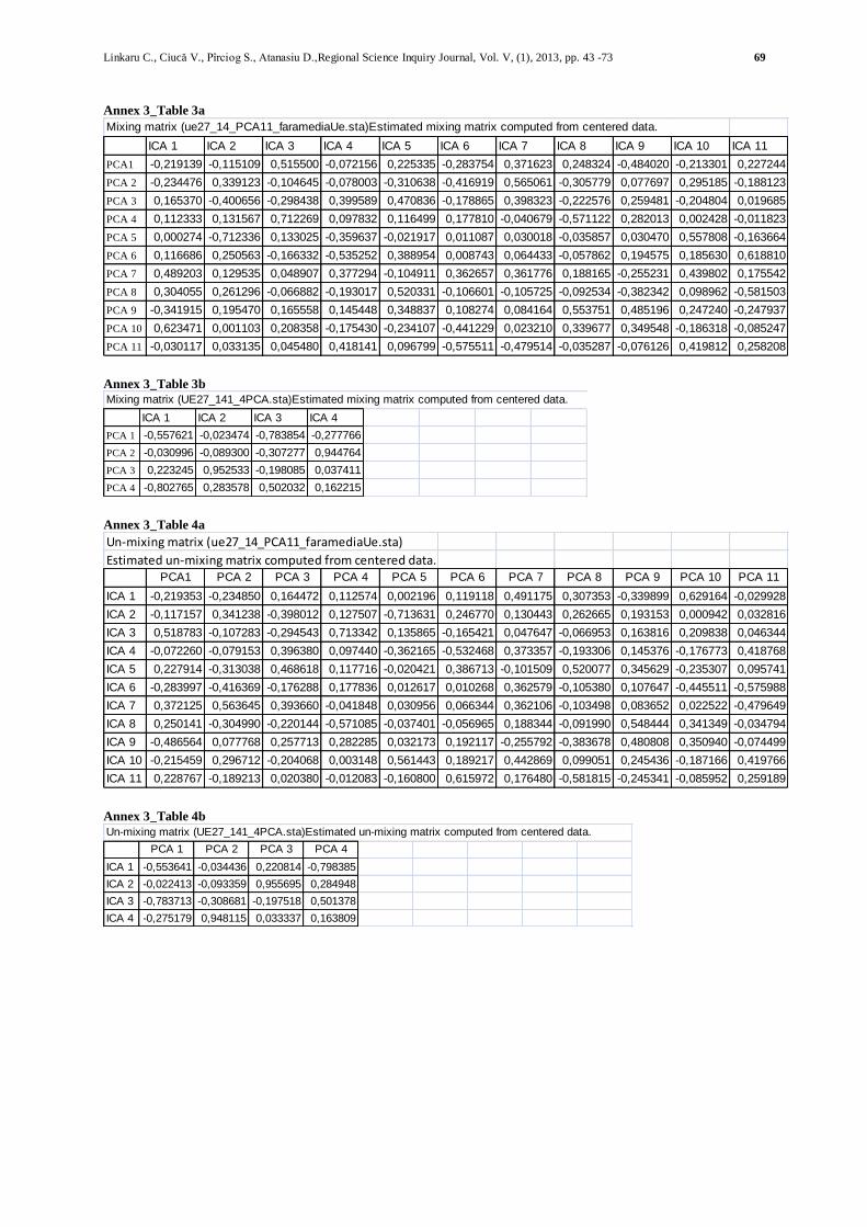
Annex 3_Table 3a
Mixing matrix (ue27_14_PCA11_faramediaUe.sta) Estimated mixing matrix computed from centered data.
ICA 1 ICA 2 ICA 3 ICA 4 ICA 5 ICA 6 ICA 7 ICA 8 ICA 9 ICA 10 ICA 11
PCA1 -0,219139 -0,115109 0,515500 -0,072156 0,225335 -0,283754 0,371623 0,248324 -0,484020 -0,213301 0,227244
PCA 2 -0,234476 0,339123 -0,104645 -0,078003 -0,310638 -0,416919 0,565061 -0,305779 0,077697 0,295185 -0,188123
PCA 3 0,165370 -0,400656 -0,298438 0,399589 0,470836 -0,178865 0,398323 -0,222576 0,259481 -0,204804 0,019685
PCA 4 0,112333 0,131567 0,712269 0,097832 0,116499 0,177810 -0,040679 -0,571122 0,282013 0,002428 -0,011823
PCA 5 0,000274 -0,712336 0,133025 -0,359637 -0,021917 0,011087 0,030018 -0,035857 0,030470 0,557808 -0,163664
PCA 6 0,116686 0,250563 -0,166332 -0,535252 0,388954 0,008743 0,064433 -0,057862 0,194575 0,185630 0,618810
PCA 7 0,489203 0,129535 0,048907 0,377294 -0,104911 0,362657 0,361776 0,188165 -0,255231 0,439802 0,175542
PCA 8 0,304055 0,261296 -0,066882 -0,193017 0,520331 -0,106601 -0,105725 -0,092534 -0,382342 0,098962 -0,581503
PCA 9 -0,341915 0,195470 0,165558 0,145448 0,348837 0,108274 0,084164 0,553751 0,485196 0,247240 -0,247937
PCA 10 0,623471 0,001103 0,208358 -0,175430 -0,234107 -0,441229 0,023210 0,339677 0,349548 -0,186318 -0,085247
PCA 11 -0,030117 0,033135 0,045480 0,418141 0,096799 -0,575511 -0,479514 -0,035287 -0,076126 0,419812 0,258208 Annex 3_Table 3b
Mixing matrix (UE27_141_4PCA.sta) Estimated mixing matrix computed from centered data.
ICA 1 ICA 2 ICA 3 ICA 4
PCA 1 -0,557621 -0,023474 -0,783854 -0,277766
PCA 2 -0,030996 -0,089300 -0,307277 0,944764
PCA 3 0,223245 0,952533 -0,198085 0,037411
PCA 4 -0,802765 0,283578 0,502032 0,162215 Annex 3_Table 4a
Un-mixing matrix (ue27_14_PCA11_faramediaUe.sta)
Estimated un-mixing matrix computed from centered data.PCA1 PCA 2 PCA 3 PCA 4 PCA 5 PCA 6 PCA 7 PCA 8 PCA 9 PCA 10 PCA 11
ICA 1 -0,219353 -0,234850 0,164472 0,112574 0,002196 0,119118 0,491175 0,307353 -0,339899 0,629164 -0,029928
ICA 2 -0,117157 0,341238 -0,398012 0,127507 -0,713631 0,246770 0,130443 0,262665 0,193153 0,000942 0,032816
ICA 3 0,518783 -0,107283 -0,294543 0,713342 0,135865 -0,165421 0,047647 -0,066953 0,163816 0,209838 0,046344
ICA 4 -0,072260 -0,079153 0,396380 0,097440 -0,362165 -0,532468 0,373357 -0,193306 0,145376 -0,176773 0,418768
ICA 5 0,227914 -0,313038 0,468618 0,117716 -0,020421 0,386713 -0,101509 0,520077 0,345629 -0,235307 0,095741
ICA 6 -0,283997 -0,416369 -0,176288 0,177836 0,012617 0,010268 0,362579 -0,105380 0,107647 -0,445511 -0,575988
ICA 7 0,372125 0,563645 0,393660 -0,041848 0,030956 0,066344 0,362106 -0,103498 0,083652 0,022522 -0,479649
ICA 8 0,250141 -0,304990 -0,220144 -0,571085 -0,037401 -0,056965 0,188344 -0,091990 0,548444 0,341349 -0,034794
ICA 9 -0,486564 0,077768 0,257713 0,282285 0,032173 0,192117 -0,255792 -0,383678 0,480808 0,350940 -0,074499
ICA 10 -0,215459 0,296712 -0,204068 0,003148 0,561443 0,189217 0,442869 0,099051 0,245436 -0,187166 0,419766
ICA 11 0,228767 -0,189213 0,020380 -0,012083 -0,160800 0,615972 0,176480 -0,581815 -0,245341 -0,085952 0,259189 Annex 3_Table 4b
Un-mixing matrix (UE27_141_4PCA.sta) Estimated un-mixing matrix computed from centered data.
PCA 1 PCA 2 PCA 3 PCA 4
ICA 1 -0,553641 -0,034436 0,220814 -0,798385
ICA 2 -0,022413 -0,093359 0,955695 0,284948
ICA 3 -0,783713 -0,308681 -0,197518 0,501378
ICA 4 -0,275179 0,948115 0,033337 0,163809
70 Linkaru C., Ciucă V., Pîrciog S., Atanasiu D.,Regional Science Inquiry Journal, Vol. V, (1), 2013, pp. 43 -73
Annex 3_Table 5a
Pre-whitening matrix (ue27_14_PCA11_faramediaUe.sta)
PCA1 PCA 2 PCA 3 PCA 4 PCA 5 PCA 6 PCA 7 PCA 8 PCA 9 PCA 10 PCA 11
ICA 1 1,002669 -0,001546 0,000317 0,000251 0,000149 -0,000026 -0,000058 0,000110 -0,000011 0,000042 -0,000095
ICA 2 -0,001546 1,000663 -0,001427 -0,001151 -0,000216 0,000048 0,000040 0,000182 0,000079 -0,000097 -0,000032
ICA 3 0,000317 -0,001427 0,995952 0,000600 -0,000056 0,000280 -0,000140 -0,000021 0,000302 0,000052 0,000014
ICA 4 0,000251 -0,001151 0,000600 1,000245 0,001788 -0,000263 -0,000417 -0,000060 -0,000016 0,000057 0,000310
ICA 5 0,000149 -0,000216 -0,000056 0,001788 1,001964 0,002154 0,001045 -0,000375 0,000058 0,000191 -0,000011
ICA 6 -0,000026 0,000048 0,000280 -0,000263 0,002154 0,997694 0,002571 0,000246 -0,000286 0,000066 -0,000038
ICA 7 -0,000058 0,000040 -0,000140 -0,000417 0,001045 0,002571 1,000496 0,001694 0,000138 0,000061 0,000022
ICA 8 0,000110 0,000182 -0,000021 -0,000060 -0,000375 0,000246 0,001694 1,000795 -0,000463 0,000701 -0,000968
ICA 9 -0,000011 0,000079 0,000302 -0,000016 0,000058 -0,000286 0,000138 -0,000463 0,995616 -0,000651 0,000240
ICA 10 0,000042 -0,000097 0,000052 0,000057 0,000191 0,000066 0,000061 0,000701 -0,000651 1,003784 0,000655
ICA 11 -0,000095 -0,000032 0,000014 0,000310 -0,000011 -0,000038 0,000022 -0,000968 0,000240 0,000655 1,000310 Annex 3_Table 5b
Pre-whitening matrix (UE27_141_4PCA.sta)
PCA 1 PCA 2 PCA 3 PCA 4
ICA 1 0,998472 0,001088 0,000978 -0,001193
ICA 2 0,001088 1,002049 -0,002123 0,000719
ICA 3 0,000978 -0,002123 1,001114 0,001231
ICA 4 -0,001193 0,000719 0,001231 0,998410 Annex 3_Table 6a
Covariance matrix (ue27_14_PCA11_faramediaUe.sta) The covariance matrix of centered and standardized (if specified) data.
PCA1 PCA 2 PCA 3 PCA 4 PCA 5 PCA 6 PCA 7 PCA 8 PCA 9 PCA 10 PCA 11
PCA1 1,000000 0,006647 -0,000512 -0,000001 0,000000 0,000000 0,000000 0,000000 0,000000 0,000000 0,000000
PCA 2 0,006647 1,000000 -0,003913 -0,000006 0,000000 0,000000 0,000000 0,000000 0,000000 0,000000 0,000000
PCA 3 -0,000512 -0,003913 1,000000 0,001145 -0,000026 -0,000016 -0,000021 0,000009 -0,000003 0,000001 0,000000
PCA 4 -0,000001 -0,000006 0,001145 1,000000 -0,004613 -0,000546 0,000005 0,000000 0,000000 0,000000 0,000000
PCA 5 0,000000 0,000000 -0,000026 -0,004613 1,000000 -0,005489 0,000087 0,000000 -0,000002 0,000000 0,000000
PCA 6 0,000000 0,000000 -0,000016 -0,000546 -0,005489 1,000000 -0,005572 0,000067 0,000270 -0,000021 -0,000015
PCA 7 0,000000 0,000000 -0,000021 0,000005 0,000087 -0,005572 1,000000 0,004960 0,000017 0,000021 -0,000003
PCA 8 0,000000 0,000000 0,000009 0,000000 0,000000 0,000067 0,004960 1,000000 0,003842 0,001970 -0,000325
PCA 9 0,000000 0,000000 -0,000003 0,000000 -0,000002 0,000270 0,000017 0,003842 1,000000 0,006191 -0,000082
PCA 10 0,000000 0,000000 0,000001 0,000000 0,000000 -0,000021 0,000021 0,001970 0,006191 1,000000 -0,004807
PCA 11 0,000000 0,000000 0,000000 0,000000 0,000000 -0,000015 -0,000003 -0,000325 -0,000082 -0,004807 1,000000 Annex 3_Table 6b
Covariance matrix (UE27_141_4PCA.sta) The covariance matrix of centered and standardized (if specified) data.
PCA 1 PCA 2 PCA 3 PCA 4
PCA 1 1,000000 0,006647 -0,000512 -0,000001
PCA 2 0,006647 1,000000 -0,003913 -0,000006
PCA 3 -0,000512 -0,003913 1,000000 0,001145
PCA 4 -0,000001 -0,000006 0,001145 1,000000 Covariance measure dependence of x on y, non normalised, where x, y are independent.
Linkaru C., Ciucă V., Pîrciog S., Atanasiu D.,Regional Science Inquiry Journal, Vol. V, (1), 2013, pp. 43 -73 71
Eigenvalues are equal to variance of projections along corresponding eigenvector (σ2= ξ) Eigenvectors of a symmetric matrix
are orthogonal, normalized basis vectors for a coordinate system. Total variance in data is given by sum of eigenvalues. 33
2
1
2
2
2
1
0
0
0
0
C
Annex 3_Table 7a
Mean Variance Minimum Maximum Mean Variance Minimum Maximum
ICA 1 0,000000 0,999385 -3,97801 1,934869 PCA1 0,000000 10,23803 -3,97392 7,032930
ICA 2 0,000000 0,998537 -0,92013 4,477845 PCA 2 0,000000 8,58839 -5,57076 3,936121
ICA 3 0,000000 0,999532 -1,45835 3,665043 PCA 3 0,000000 5,22154 -3,32295 4,364150
ICA 4 0,000000 0,995466 -2,79739 1,896845 PCA 4 0,000000 1,01539 -2,31210 3,822250
ICA 5 0,000000 0,996458 -4,03926 1,499888 PCA 5 0,000000 0,54612 -2,22974 1,838798
ICA 6 0,000000 1,005686 -3,48735 1,948706 PCA 6 0,000000 0,38975 -1,40335 1,334375
ICA 7 0,000000 0,996886 -2,06508 3,567277 PCA 7 0,000000 0,26260 -1,06926 0,974273
ICA 8 0,000000 1,005739 -1,72374 3,954616 PCA 8 0,000000 0,19164 -1,19199 0,961533
ICA 9 0,000000 1,001332 -3,18592 2,634494 PCA 9 0,000000 0,12364 -1,04479 0,921608
ICA 10 0,000000 1,000690 -3,99528 1,696116 PCA 10 0,000000 0,09917 -0,70351 0,799567
ICA 11 0,000000 1,000859 -1,34836 3,559213 PCA 11 0,000000 0,07257 -0,74287 0,817664
Descriptive statistics of separated source data
(ue27_14_PCA11_faramediaUe.sta)
Number of components: 11
Number of valid cases: 141
Descriptive statistics for variables
(ue27_14_PCA11_faramediaUe.sta)
Number of valid cases: 141
Annex 3_Table 7b
33
***, Why is dimensionality reduction useful?, http://rieke-server.physiol.washington.edu/People/Fred/Classes/545/PCA2.pdf
Mean Variance Minimum Maximum Mean Variance Minimum Maximum
ICA 1 0,000000 1,001693 -1,83510 1,575418 PCA 1 0,000000 10,23803 -3,97392 7,032930
ICA 2 0,000000 0,998915 -2,37548 2,055181 PCA 2 0,000000 8,58839 -5,57076 3,936121
ICA 3 0,000000 1,000186 -1,29439 4,432552 PCA 3 0,000000 5,22154 -3,32295 4,364150
ICA 4 0,000000 0,999267 -1,73535 1,388644 PCA 4 0,000000 1,01539 -2,31210 3,822250
Descriptive statistics for variables
(UE27_141_4PCA.sta)
Number of valid cases: 141
Descriptive statistics of separated source data
(UE27_141_4PCA.sta)
Number of components: 4
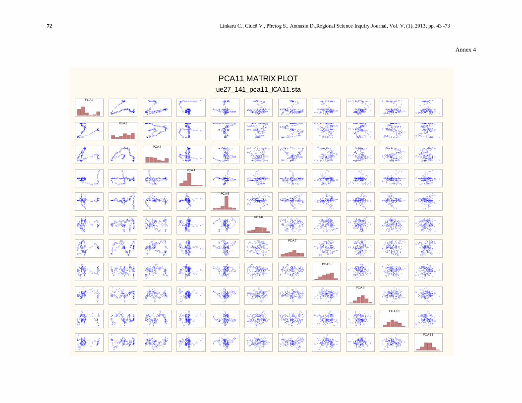
72 Linkaru C., Ciucă V., Pîrciog S., Atanasiu D.,Regional Science Inquiry Journal, Vol. V, (1), 2013, pp. 43 -73
Annex 4
PCA11 MATRIX PLOT
ue27_141_pca11_ICA11.sta
PCA1
PCA 2
PCA 3
PCA 4
PCA 5
PCA 6
PCA 7
PCA 8
PCA 9
PCA 10
PCA 11
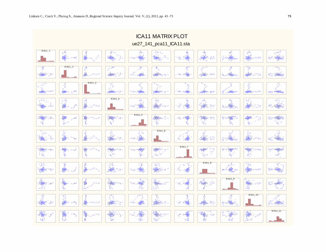
Linkaru C., Ciucă V., Pîrciog S., Atanasiu D.,Regional Science Inquiry Journal, Vol. V, (1), 2013, pp. 43 -73 73
ICA11 MATRIX PLOT
ue27_141_pca11_ICA11.sta
ICA11_ 1
ICA11_ 2
ICA11_3
ICA11_4
ICA11_5
ICA11_6
ICA11_7
ICA11_8
ICA11_9
ICA11_10
ICA11_11