Embed Size (px)
Citation preview

Finding Lie Symmetries of PDEs with MATHEMATICA:Applications to Nonlinear Fiber Optics
Vladimir PulovDepartment of Physics, Technical University-Varna, Bulgaria
Ivan UzunovDepartment of Applied Physics, Technical University-Sofia, Bulgaria
Eddy ChacarovDepartment of Informatics and Mathematics, Varna Free University, Bulgaria
Geometry, Geometry, IntegrabilityIntegrability and and QuatizationQuatization −− June 8June 8--13, 200713, 2007
Plan of Presentation
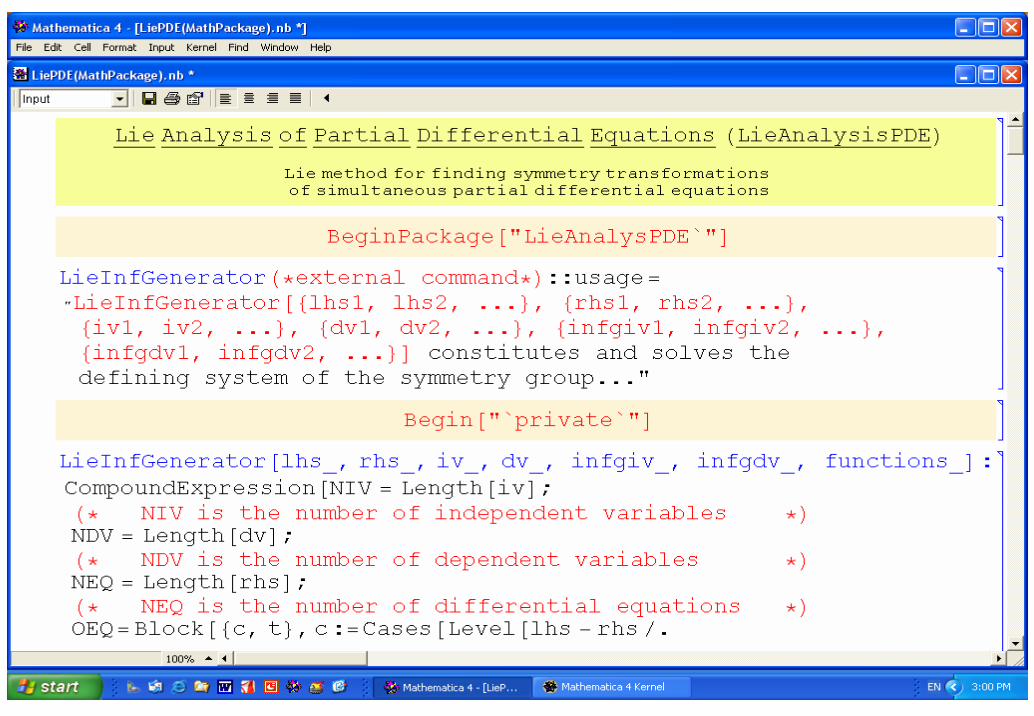
1. MATHEMATICA package for finding Lie symmetries of PDE1.1. Block-scheme and algorithm1.2. Input and output 1.3. Tracing the evaluation1.4. Trial run
2. Applications to nonlinear fiber optics2.1. Physical model2.2. Results obtained
3. Conclusion
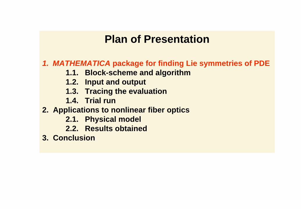
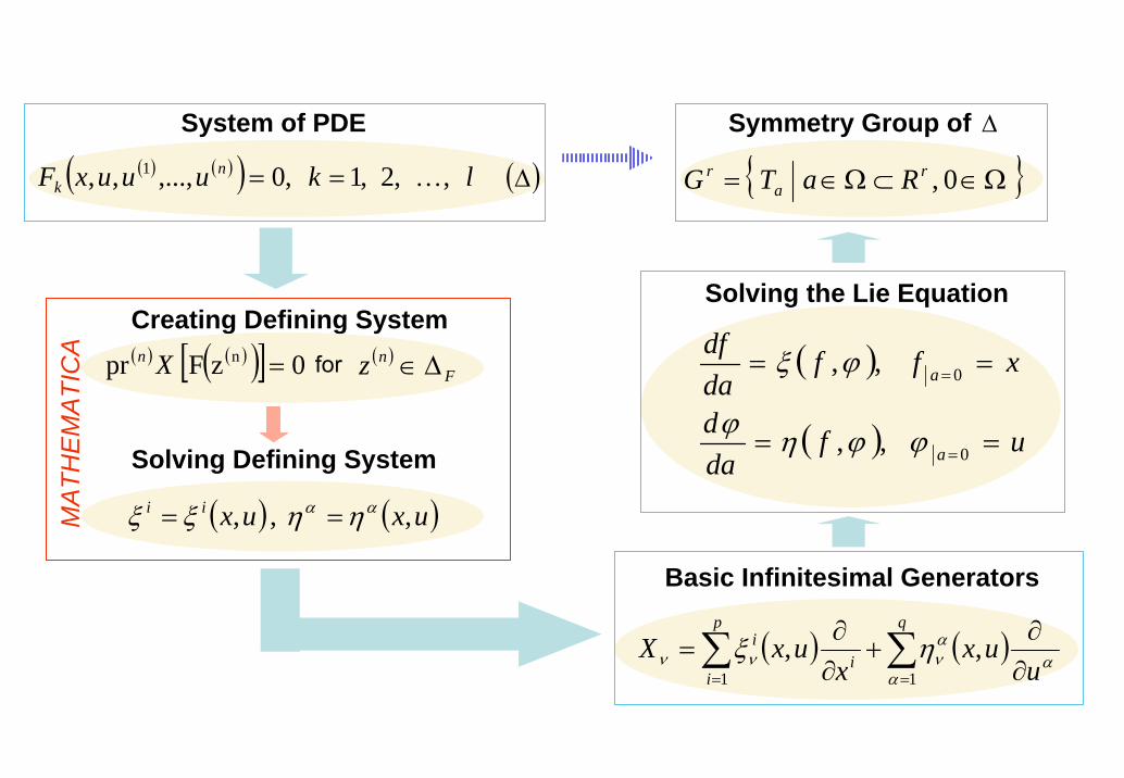
Symmetry Group of Δ
{ } 0 , Ω∈⊂Ω∈= ra
r RaTG
System of PDE( ) ( )( ) lkuuuxF n
k ,,2,1,0,...,,, 1 K== ( )Δ
Creating Defining System( ) ( )( )[ ] 0zF pr n =Xn for
Solving Defining System
( ) ( )uxuxii , , , αα ηηξξ ==
( )F
nz Δ∈
MA
THE
MA
TIC
A ( )
( ) ufdad
xffdadf
a
a
==
==
=
=
0
0
,,
,,
ϕϕηϕ
ϕξ
Solving the Lie Equation
( ) ( )∑∑== ∂
∂+
∂∂
=qp
ii
i
uux
xuxX
11,,
αα
αννν ηξ
Basic Infinitesimal Generators

Each solution of after transformation of the group remains a solution of .G ΔΔ
Lie Group of Symmetry Transformations
( ) ( )( ) lkuuuxF nk ,,2,1,0,...,,, 1 K==
{ } 0 , δδ ∈⊂∈= RaTG a
( )Δ
u
x
( )xfu =u′
x′
( )xfu ′′=′aT
If is a solution of then is also a solution of .fTf a ⋅=′ Δf Δ
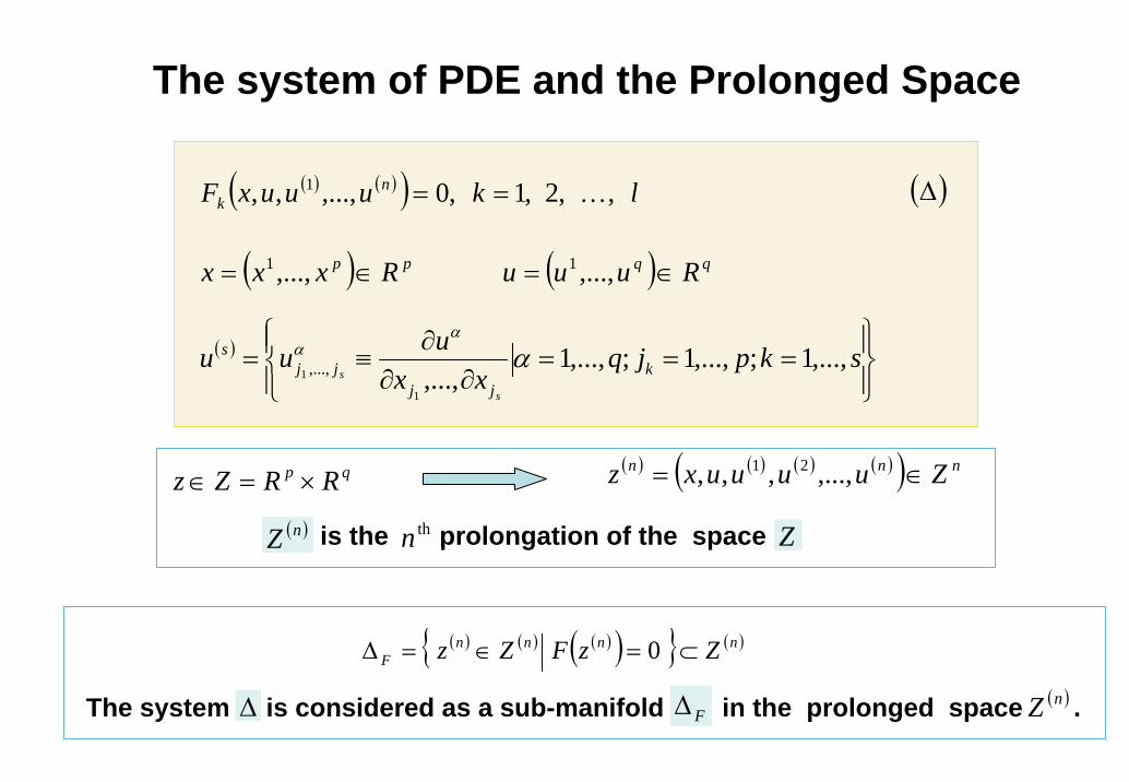
The system of PDE and the Prolonged Space
( ) ( )( ) lkuuuxF nk ,,2,1,0,...,,, 1 K==
( ) pp Rxxx ∈= ,...,1 ( ) qq Ruuu ∈= ,...,1
( )
⎪⎭
⎪⎬⎫
⎪⎩
⎪⎨⎧
===∂∂
∂≡= skpjq
xxuuu k
jjjj
s
s
s,...,1;,...,1;,...,1
,...,1
1 ,..., αα
α
( )Δ
( ) ( ) ( ) ( )( ) nnn Zuuuuxz ∈= ,...,,,, 21qp RRZz ×=∈
is the prolongation of the space Z( )nZ thn
( ) ( ) ( )( ){ } ( )nnnnF ZzFZz ⊂=∈=Δ 0
The system is considered as a sub-manifold in the prolonged space . FΔΔ ( )nZ
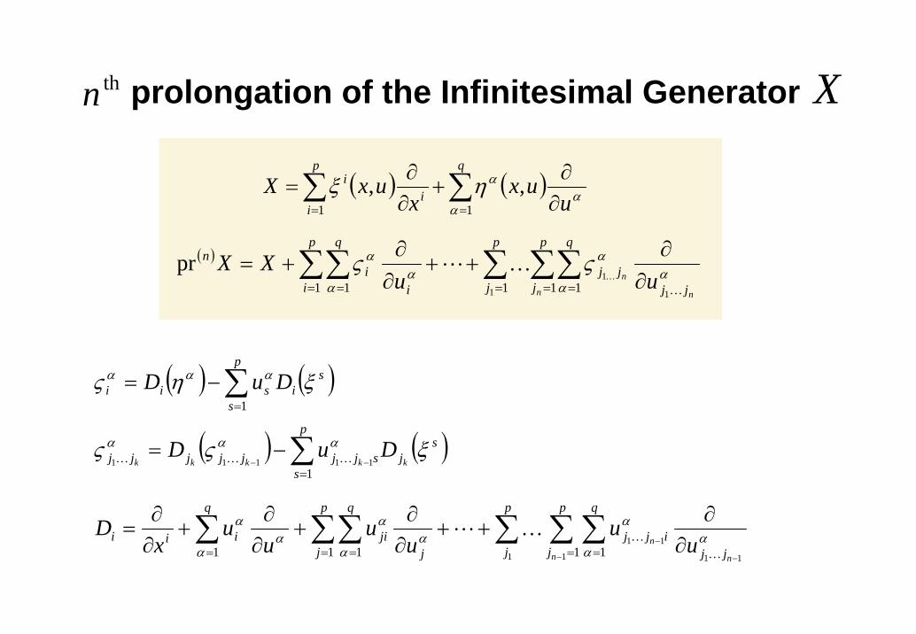
prolongation of the Infinitesimal Generatorthn X
( ) ∑∑∑∑∑= === = ∂
∂++
∂∂
+=p
j
q
jjjj
p
ji
p
i
q
in
n n
n uuXX
1 111 1 1
1
1
prα
αα
αα
α ςςK
KKL
( ) ( )∑=
−=p
s
sisii DuD
1ξης ααα
( ) ( )sj
p
ssjjjjjjj kkkkkDuD ξςς ααα ∑
=−−
−=1
11111 KKK
∑ ∑ ∑∑∑∑= == == − −
− ∂∂
++∂∂
+∂∂
+∂∂
=p
j
p
j
q
jjijj
p
j
q
jji
q
iiin n
n uu
uu
uu
xD
1 1 11
111 11 11 α
αα
αα
α
αα
α
K
KKL
( ) ( ) αα
αηξu
uxx
uxXq
i
p
i
i
∂∂
+∂∂
= ∑∑==
,,11
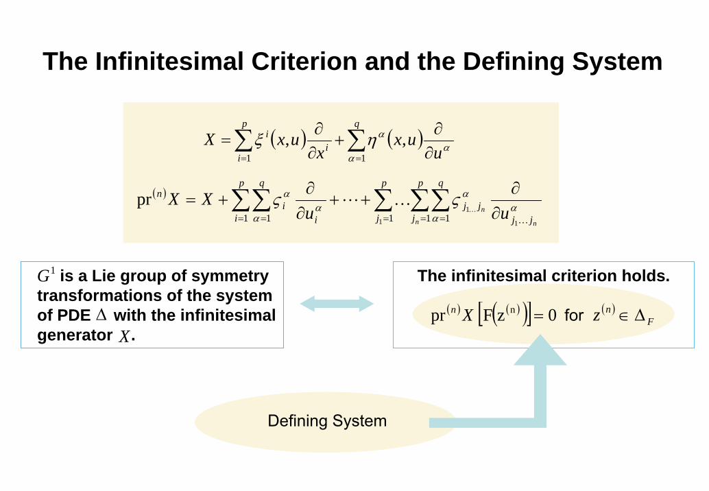
The Infinitesimal Criterion and the Defining System
( ) ∑∑∑∑∑= === = ∂
∂++
∂∂
+=p
j
q
jjjj
p
ji
p
i
q
in
n n
n uuXX
1 111 1 1
1
1
prα
αα
αα
α ςςK
KKL
( ) ( ) αα
αηξu
uxx
uxXq
i
p
i
i
∂∂
+∂∂
= ∑∑==
,,11
is a Lie group of symmetry transformations of the system of PDE with the infinitesimalgenerator .
1G
ΔX
The infinitesimal criterion holds.
for ( )F
nz Δ∈( ) ( )( )[ ] 0zF pr n =Xn
Defining System
Symmetry Group of Δ
{ } 0 , Ω∈⊂Ω∈= ra
r RaTG
System of PDE( ) ( )( ) lkuuuxF n
k ,,2,1,0,...,,, 1 K== ( )Δ
Creating Defining System( ) ( )( )[ ] 0zF pr n =Xn for
Solving Defining System
( ) ( )uxuxii , , , αα ηηξξ ==
( )F
nz Δ∈
MA
THE
MA
TIC
A ( )
( ) ufdad
xffdadf
a
a
==
==
=
=
0
0
,,
,,
ϕϕηϕ
ϕξ
Solving the Lie Equation
( ) ( )∑∑== ∂
∂+
∂∂
=qp
ii
i
uux
xuxX
11,,
αα
αννν ηξ
Basic Infinitesimal Generators

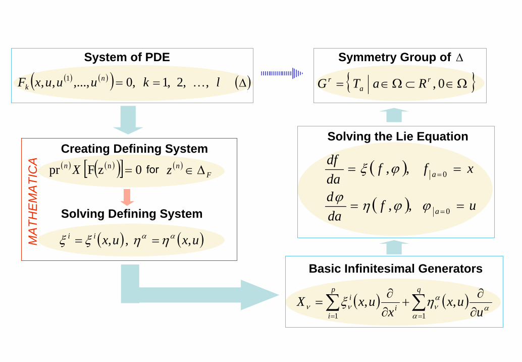
Data Input
Basic Setup
EquivalentTransformations
Block
Solvers Block
Data Output
At least one equation has been solved.
Creating Defining System
Solving Procedure
False
True
MA
TH
EM
AT
IC
A
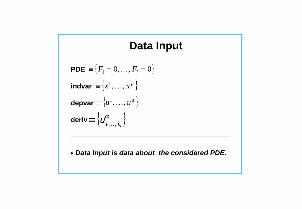
Data Input
PDE
indvar
depvar
deriv
_________________________________________
• Data Input is data about the considered PDE.
{ }αsjju ,,1
K≡
{ }0 , ,01 ==≡ lFF K
{ }pxx , ,1 K≡
{ }quu , ,1 K≡
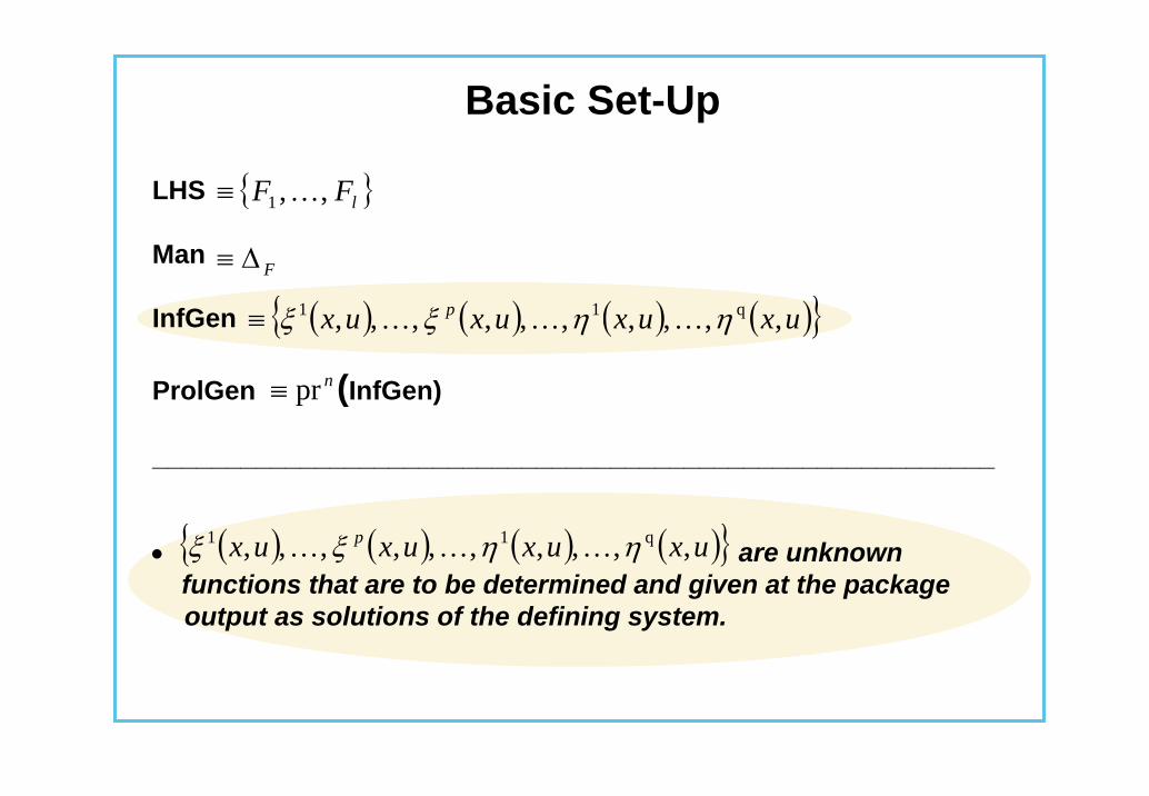
Basic Set-Up
LHS
Man
InfGen
ProlGen (InfGen)
_________________________________________________________
• are unknown functions that are to be determined and given at the package output as solutions of the defining system.
{ }lFF , ,1 K≡
FΔ≡
( ) ( ) ( ) ( ){ }uxuxuxux p , , ,, , ,, , ,, q11 ηηξξ KKK≡
( ) ( ) ( ) ( ){ }uxuxuxux p , , ,, , ,, , ,, q11 ηηξξ KKK
npr≡

Creating Defining System
________________________________________________________________
• Defining System is the major object in the program.• Defining System is created by applying the infinitesimal
criterion InfGen (LHS) |Man=0.• Defining System consists of linear partial differential equations.
Defining SystemInfinitesimal Criterion
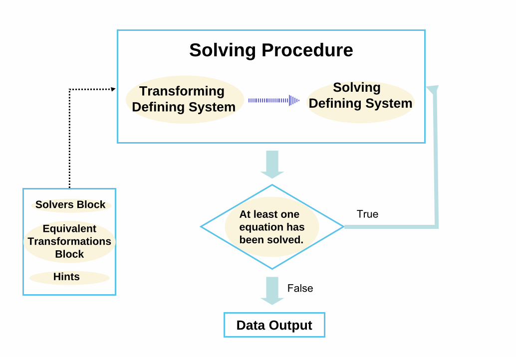
At least one equation has been solved.
Data Output
False
True
Solving Procedure
TransformingDefining System
Solving Defining System
EquivalentTransformations
Block
Solvers Block
Hints
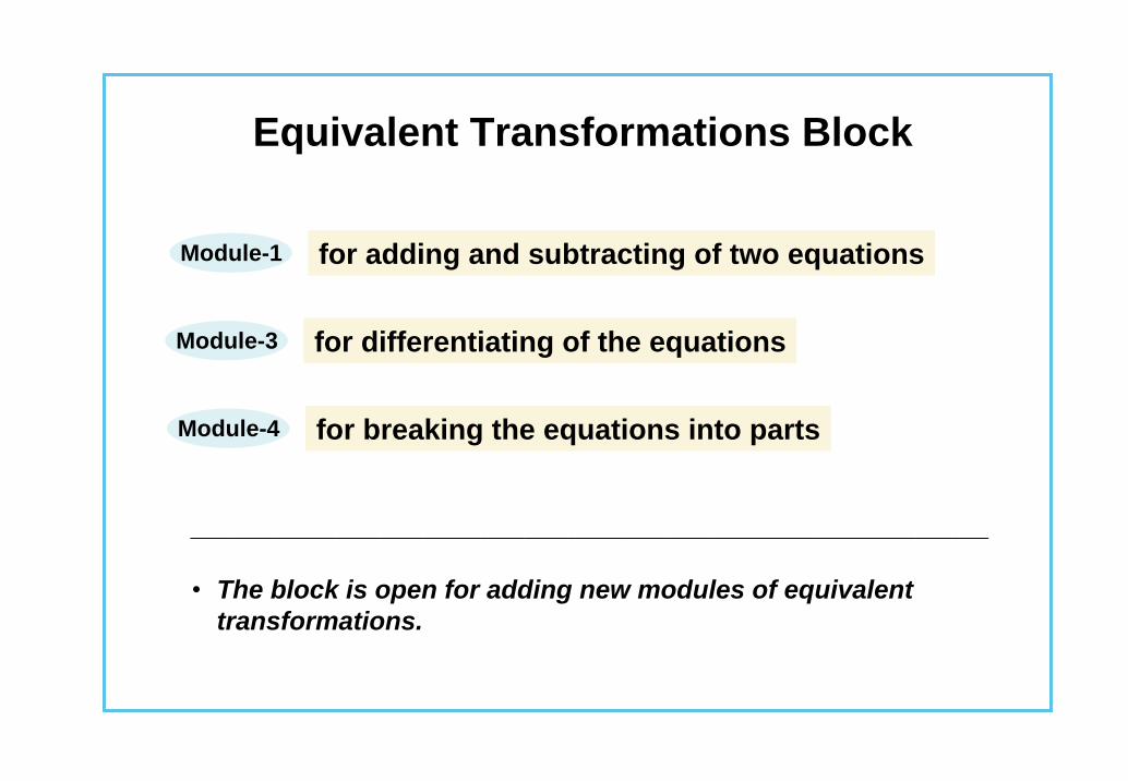
Equivalent Transformations Block
_______________________________________________________
• The block is open for adding new modules of equivalent transformations.
for breaking the equations into partsModule-4
for differentiating of the equationsModule-3
for adding and subtracting of two equationsModule-1

Solvers Block
_______________________________________________________
• The block is open for adding new modules for solving equations.
solver of Module-4
solver of Module-3
solver of Module-2
solver of Module-1 021 =+CxC
Module-5 solver of
021 =+ yCxC
021 =+′ CyC
021 =+′′ CyC
021 =+′′′ CyC
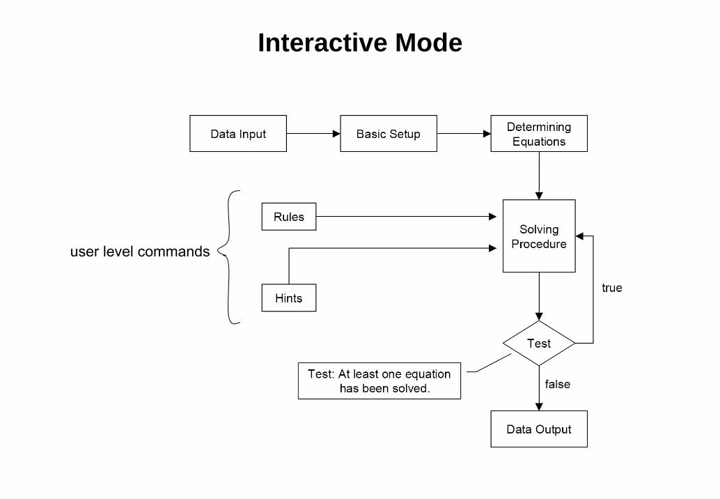
Interactive Mode
user level commands
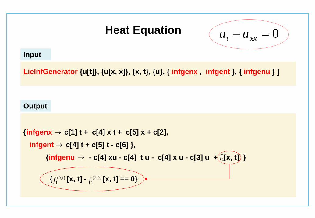
Heat Equation 0=− xxt uu
LieInfGenerator {u[t]}, {u[x, x]}, {x, t}, {u}, { infgenx , infgent }, { infgenu } ]
Input
Output
{infgenx c[1] t + c[4] x t + c[5] x + c[2],
infgent c[4] t + c[5] t - c[6] },
{infgenu - c[4] xu - c[4] t u - c[4] x u - c[3] u + [x, t] }
{ [x, t] - [x, t] == 0}
→
→
→
( )1,01f
( )0,21f
1f

Heat equation0=− xxt uu
Tracing the Evaluation
021 =+CxC
021 =+′ CyC
021 =+′′ CyC
021 =+′′′ CyC
021 =+ yCxC
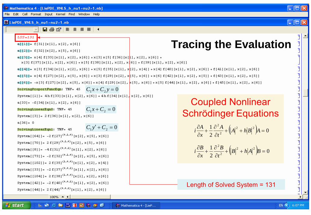
Tracing the Evaluation
Coupled Nonlinear Schrödinger Equations
( ) 021 22
2
2
=++∂∂
+∂∂ ABhA
tA
xAi
( ) 021 22
2
2
=++∂∂
+∂∂ BAhB
tB
xBi
Length of Solved System = 131
021 =+′ CyC
021 =+CxC
021 =+ yCxC
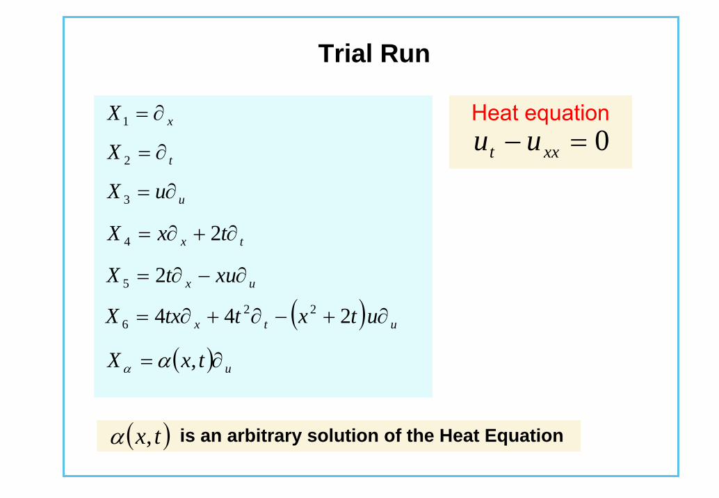
Trial Run
Heat equation0=− xxt uu
is an arbitrary solution of the Heat Equation ( )tx,α
xX ∂=1
tX ∂=2
uuX ∂=3
tx txX ∂+∂= 24
ux xutX ∂−∂= 25
( ) utx utxttxX ∂+−∂+∂= 244 226
( ) utxX ∂= ,αα

Trial RunKdV equation
0=++ xxxxt uuuu
time translation
xX ∂=1
tX ∂=2
uxtX ∂+∂=3
utx utxX ∂−∂+∂= 234
space translation
( ) ( )ε−= txfu ,2
( ) ( ) εε +−= ttxfu ,3
( ) ( )texefeu εεε 324 , −−−=dilation
Galilean boost
is an arbitrary solution of the KdV Equation is the group parameter
( )txfu ,=R∈ε
( ) ( )txfu ,1 ε−=

References
[1] Schwarz, F., Computing 34 (1985) 91.[2] Baumann, G., Math. Comp. Simulation 48 (1998) 205.[3] Baumann, G., Lie Symmetries of Differential equations: a MATHEMATICA
Program to Determine Lie Symmetries, at www.library.wolfram.com/infocenter/MathSource/431.

Application to Fiber Optics(physical model)
Coupled Nonlinear Schrödinger Equations (CNSEs)
021
2222
2
2
=+⎟⎟
⎠
⎞
⎜⎜
⎝
⎛
∂
∂−
∂
∂−++
∂∂
+∂∂ BA
tB
tA
BAtA
xAi σθθγ
02
2222
2
2
=+⎟⎟
⎠
⎞
⎜⎜
⎝
⎛
∂
∂−
∂
∂−++
∂∂
+∂∂ AB
tB
tA
ABtB
xBi σθθγν
weak birefringent fibers
two-mode fibers
strong birefringent fibers
Raman gain coefficient
0≠σ
2 ,0 == γσ
32 ,0 == γσθ

Lie Group AnalysisLie Group Analysis
tX
∂∂
=1 xX
∂∂
=2 α∂∂
=3X βν
α ∂∂
+∂∂
+∂∂
= ttt
xX 5 ςς∂∂
+∂∂
+∂∂
−∂∂
−=z
zx
xt
tX 26β∂∂
=4X
1att +=′2axx +=′ 3a+=′ αα 4a+=′ ββ
xatt 5+=′
xa
ta2
25
5 ++=′ αα
xa
ta2
25
5ν
νββ ++=′
( )6exp att −=′
( )62exp axx −=′
( )6exp azz =′
( )6exp aξξ =′
grou
psgr
oups
alge
bras
alge
bras
2T 3T 4T
5T6T
1T
( ) ( )βςα iBizA expexp ==
Admitted Lie point symmetries
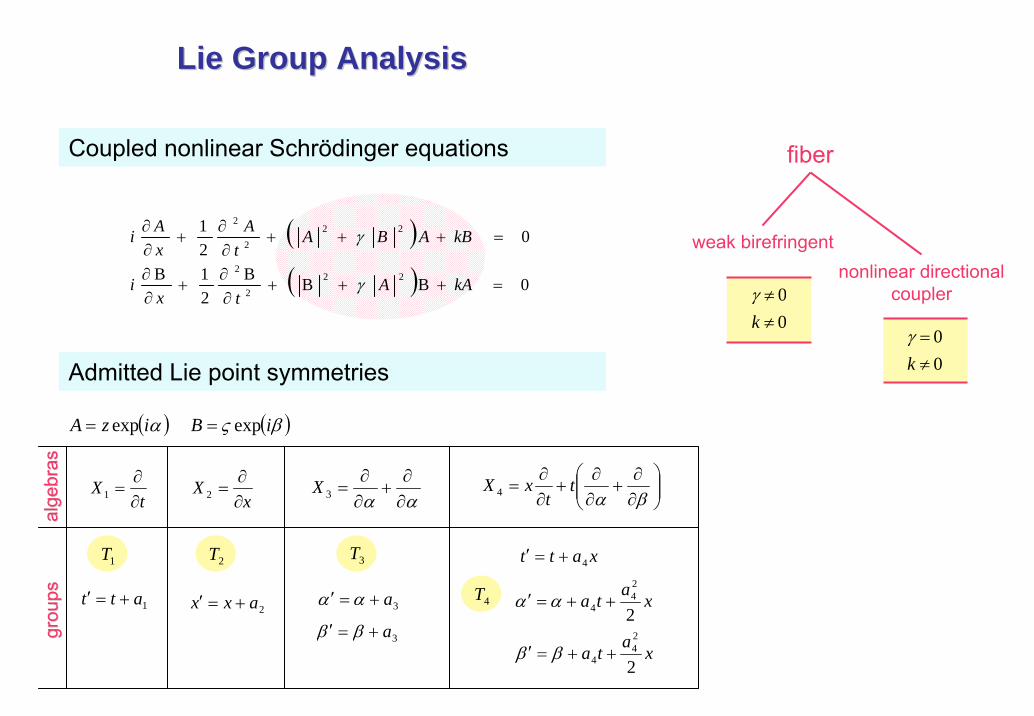
Coupled nonlinear Schrödinger equations
( )( ) 0BBB
2B
021
22
2
2
22
2
2
=++∂∂
+∂∂
=++∂∂
+∂∂
Atx
i
ABAt
AxAi
γν
γ
group velocity dispersion
positive
1−=νnegative
1+=ν
optical fiber
two mode
2=γ
strong birefringent
32
=γ

tX
∂∂
=1 xX
∂∂
=2 α∂∂
=3X ⎟⎟⎠
⎞⎜⎜⎝
⎛∂∂
+∂∂
+∂∂
=βα
tt
xX 5β∂∂
=4X
1att +=′2axx +=′ 3a+=′ αα 4a+=′ ββ
xatt 5+=′
xa
ta2
25
5 ++=′ αα
xa
ta2
25
5 ++=′ ββ
grou
psgr
oups
alge
bras
alge
bras
2T 3T 4T
5T
1T
( ) ( )βςα iBizA expexp ==
( ) ( )
( ) ( )0BBB
21B
021
2222
2
2
2222
2
2
=⎟⎟
⎠
⎞
⎜⎜
⎝
⎛
∂
∂−
∂
∂−++
∂∂
+∂∂
=⎟⎟
⎠
⎞
⎜⎜
⎝
⎛
∂
∂−
∂
∂−++
∂∂
+∂∂
tB
tA
Atx
i
At
Bt
ABA
tA
xAi
θθγ
θθγ
strong birefringent fiber
32
=γ
strong birefringent fiberwith parallel Raman scattering
0≠θ
Lie Group AnalysisLie Group Analysis
Coupled nonlinear Schrödinger equations
Admitted Lie point symmetries
tX
∂∂
=1 αα ∂∂
+∂∂
=3X ⎟⎟⎠
⎞⎜⎜⎝
⎛∂∂
+∂∂
+∂∂
=βα
tt
xX 4
1att +=′2axx +=′ 3a+=′ αα
3a+=′ ββ
xatt 4+=′
xata2
24
4 ++=′ αα
xata2
24
4 ++=′ ββ
grou
psgr
oups
alge
bras
alge
bras
2T 3T
4T
1T
( ) ( )βςα iBizA expexp ==
( )( ) 0BBB
21B
021
222
2
222
2
=+++∂∂
+∂∂
=+++∂∂
+∂∂
kAAtx
i
kBABAt
AxAi
γ
γ
fiber
weak birefringent
00
≠≠
kγ
nonlinear directionalcoupler
00
≠=
kγ
xX
∂∂
=2
Admitted Lie point symmetries
Coupled nonlinear Schrödinger equations
Lie Group AnalysisLie Group Analysis

SYMMETRYSYMMETRY GROUPGROUP REDUCTIONREDUCTION
optimal set of subalgebras
optimal set of reduced ODEs
optimal set of group invariant solutions
clas
sific
atio
n
adjointrepresentations
symmetrygroup
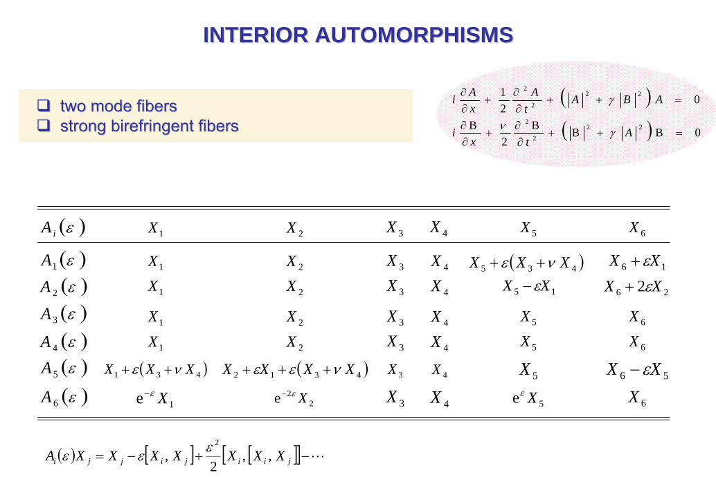
INTERIOR AUTOMORPHISMS INTERIOR AUTOMORPHISMS
( )ε1A( )ε2A
( )ε4A( )ε5A
( )ε6A
( )ε3A
( )εiA 1X
1X
1X
1X
1X
( )431 XXX νε ++
1e Xε−
2X
2X
2X
2X
2X
( )4312 XXXX νεε +++
22e Xε−
3X
3X
3X
3X
3X
3X
3X
4X
4X
4X
4X
4X
4X
4X
5X
5X
5X
15 XX ε−
5X
( )435 XXX νε ++
5e Xε
6X
6X
56 XX ε−
6X
16 XX ε+
6X
26 2 XX ε+
( ) [ ] [ ][ ] L−+−= jiijijji XXXXXXXA ,,2
,2εεε
two mode fiberstwo mode fibersstrong birefringent fibersstrong birefringent fibers
( )( ) 0BBB
2B
021
222
2
222
2
=++∂∂
+∂∂
=++∂∂
+∂∂
Atx
i
ABAt
AxAi
γν
γ

OPTIMAL SET OF SUBALGEBRASOPTIMAL SET OF SUBALGEBRAS
αεε∂∂
+∂∂
=+t
XX 31Case A
Case C
Case B ( )β
νεα
ε∂∂
++∂∂
+∂∂
=+ ttt
xXX 54
βε
αδεδ
∂∂
+∂∂
+∂∂
=++x
XXX 432
Case D ( )β
νδα
εδε∂∂
++∂∂
+∂∂
+∂∂
=++ ttxt
xXXX 542
Case E βδ
αε
ςςδε
∂∂
+∂∂
+∂∂
+∂∂
+∂∂
−∂∂
−=++z
zx
xt
tXXX 2643
Case F βδ
αεδε
∂∂
+∂∂
=+ 43 XX
1,0 ±=ε
1,0 ±=ε
R∈±=±= δεε ,1or 1,0
R∈±= δε ,1
R∈δε ,
1,or 0,1 =∈== δεδε R
two mode fiberstwo mode fibersstrong birefringent fibersstrong birefringent fibers
( )( ) 0BBB
2B
021
222
2
222
2
=++∂∂
+∂∂
=++∂∂
+∂∂
Atx
i
ABAt
AxAi
γν
γ
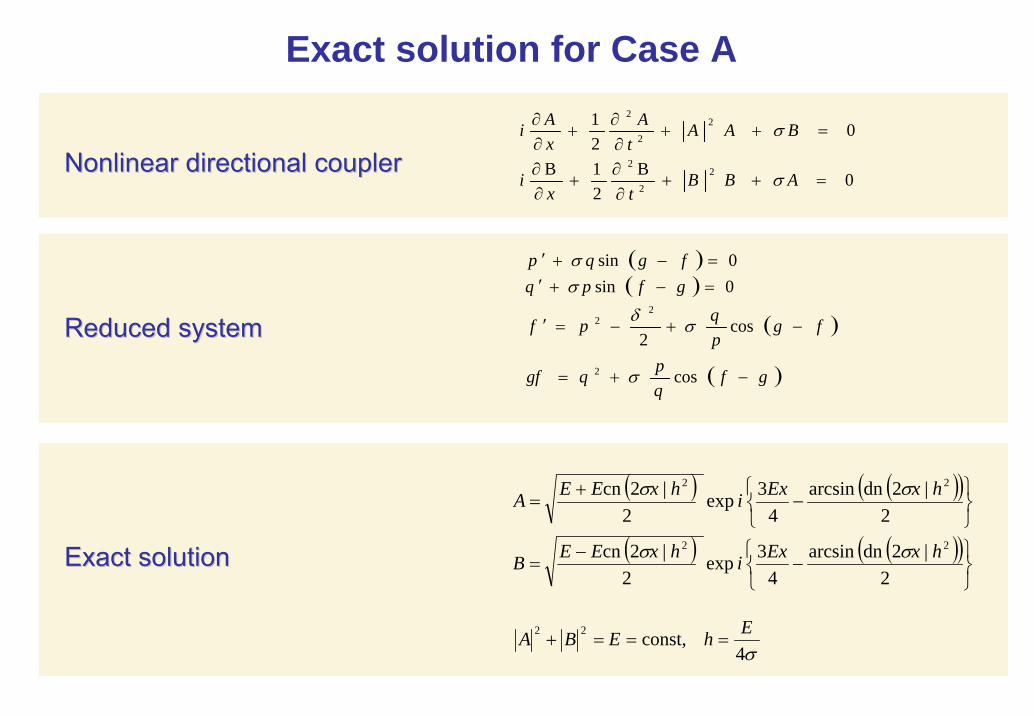
0B21B
021
22
2
22
2
=++∂∂
+∂∂
=++∂∂
+∂∂
ABBtx
i
BAAt
AxAi
σ
σ
Nonlinear directional couplerNonlinear directional coupler
Reduced systemReduced system
( )( )
( )
( )gfqpqgf
fgpqpf
gfpqfgqp
−+=
−+−=′
=−+′=−+′
cos
cos2
0sin0sin
2
22
σ
σδ
σσ
( ) ( )( )⎭⎬⎫
⎩⎨⎧
−+
=2
|2dn arcsin 4
3 exp2
|2cn 22 hxExihxEEA σσ
( ) ( )( )⎭⎬⎫
⎩⎨⎧
−−
=2
|2dn arcsin 4
3 exp2
|2cn 22 hxExihxEEB σσ
σ4const, 22 EhEBA ===+
Exact solutionExact solution
Exact solution for Case A

REDUCTION PROCESREDUCTION PROCES(Case C)(Case C)
Generator βε
αδεδ
∂∂
+∂∂
+∂∂
=++x
XXX 432 R∈±=±= δεε ,1or 1,0
two mode fiberstwo mode fibersstrong birefringent fibersstrong birefringent fibers
( )( ) 0BBB
2B
021
222
2
222
2
=++∂∂
+∂∂
=++∂∂
+∂∂
Atx
i
ABAt
AxAi
γν
γ
Invariants tJ =1 zJ =2 ς=3J xJ δα −=3 xJ εβ −=4
New variables ( )xpz =
( ) ( )βςα iBizA expexp ==
( )xq=ς ( ) xtf δα += ( ) xtg εβ +=
Reduced system ( )( ) 0222
0222
0202
232
232
=−++′−′′
=−++′−′′
=′′+′′=′′+′′
qqpqgqq
ppqpfpp
gqgqfpfp
ενγνν
δγ
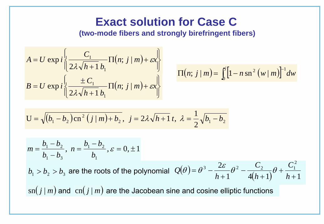
Exact solution for Case C(two-mode fibers and strongly birefringent fibers)
( )⎪⎭
⎪⎬⎫
⎪⎩
⎪⎨⎧
+Π+
= xmjnbh
CiUA ε
λ| ;
12 exp
1
1
( )⎪⎭
⎪⎬⎫
⎪⎩
⎪⎨⎧
+Π+
±= xmjn
bhC
iUB ελ
| ; 12
exp 1
1
( ) ( ) 2122
21 21 , 12 ,| cn U bbthjbmjbb −=+=+−= λλ
( ) ( )[ ] dwmwnmjnj
∫−
−=Π0
12 | sn 1| ;
1 0, , ,1
21
31
21 ±=−
=−−
= εb
bbn
bbbb
m
are the roots of the polynomial321 bbb >> ( ) ( ) 11412 2
1223
++
+−
+−=
hC
hC
hQ θθεθθ
and are the Jacobean sine and cosine elliptic functions ( )mj |sn ( )mj |cn
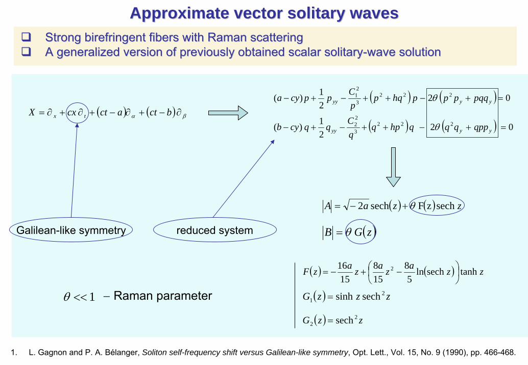
Approximate vector solitary wavesApproximate vector solitary wavesStrong birefringent fibers with Raman scattering Strong birefringent fibers with Raman scattering A generalized version of previously obtained scalar solitary-wave solutionA generalized version of previously obtained scalar solitary-wave solution
( ) ( ) zzazazazF tanh sech ln5
8158
1516 2 ⎟
⎠⎞
⎜⎝⎛ −+−=
( ) zzzG 21 sech sinh =
( ) zzG 22 sech=
( ) ( ) βα ∂−+∂−+∂+∂= bctactcxX tx
( ) ( ) sech zF sech2 zzaA θ+−=
( )zGB θ=Galilean-like symmetry reduced system
( ) ( )
( ) ( ) 0 2 21 )(
0 2 21)(
2223
22
2223
21
=+−++−+−
=+−++−+−
yyyy
yyyy
qppqqqhpqqCqqcyb
pqqppphqppCppcya
θ
θ
1. L. Gagnon and P. A. Bélanger, Soliton self-frequency shift versus Galilean-like symmetry, Opt. Lett., Vol. 15, No. 9 (1990), pp. 466-468.
1<<θ − Raman parameter
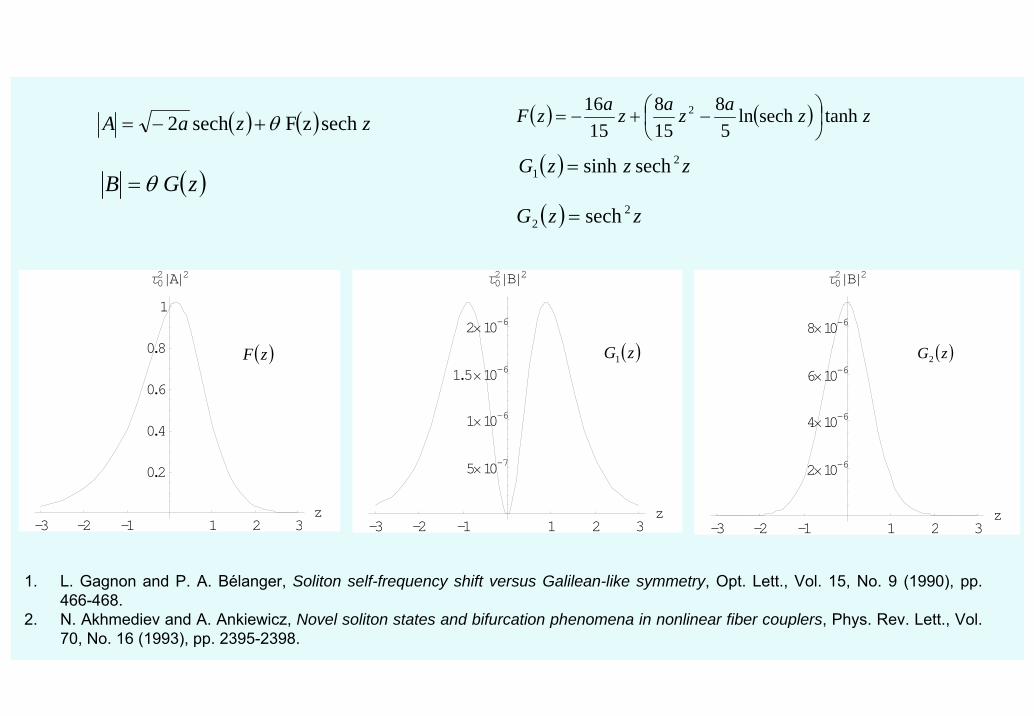
-3 -2 -1 1 2 3z
0.2
0.4
0.6
0.8
1
τ02»A»2
-3 -2 -1 1 2 3z
5×10⁻⁷
1×10⁻⁶
1.5×10⁻⁶
2×10⁻⁶
τ02»B»2
-3 -2 -1 1 2 3z
2×10⁻⁶
4×10⁻⁶
6×10⁻⁶
8×10⁻⁶
τ02»B»2
( ) ( ) zzazazazF tanh sech ln5
8158
1516 2 ⎟
⎠⎞
⎜⎝⎛ −+−=
( ) zzzG 21 sech sinh =
( ) zzG 22 sech=
( ) ( ) sech zF sech2 zzaA θ+−=
( )zGB θ=
( )zF ( )zG1 ( )zG2
1. L. Gagnon and P. A. Bélanger, Soliton self-frequency shift versus Galilean-like symmetry, Opt. Lett., Vol. 15, No. 9 (1990), pp. 466-468.
2. N. Akhmediev and A. Ankiewicz, Novel soliton states and bifurcation phenomena in nonlinear fiber couplers, Phys. Rev. Lett., Vol. 70, No. 16 (1993), pp. 2395-2398.
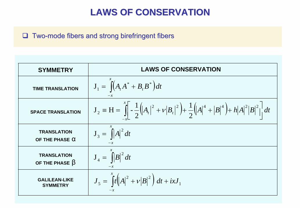
LAWSLAWS OFOF CONSERVATIONCONSERVATION
TwoTwo--modemode fibers and strongfibers and strong birefringentbirefringent fibersfibers
( )
( ) ( )
( ) 122
5
24
23
2244222
**1
J
J
21
21-HJ
J
ixJdtBAtJ
dtB
dtA
dtBAhBABA
dtBBAA
x
x
x
x
x
x
x
xtt
x
xtt
++=
=
=
⎥⎦⎤
⎢⎣⎡ ++++=≡
+=
∫
∫
∫
∫
∫
−
−
−
−
−
ν
ν
TIME TRANSLATION
SYMMETRY LAWS OF CONSERVATION
SPACE TRANSLATION
TRANSLATION OF THE PHASE α
TRANSLATION OF THE PHASE β
GALILEAN-LIKESYMMETRY
References
[1] Christodoulides, D.N. and R.I. Joseph, Optics Lett., 13(1), 53-55 (1988).[2] Tratnik, M. V. and J. E. Sipe, Phys. Rev. A, 38(4), 2011-2017 (1988).[3] Christodoulides, D.N., Phys. Lett. A, 132(8, 9), 451-452 (1988).[4] Florjanczyk, M. and R. Tremblay, Phys. Lett. A, 141(1,2), 34-36 (1989).[5] Kostov, N. A. and I. M. Uzunov, Opt. Commun., 89, 389-392 (1992).[6] Florjanczyk, M. and R. Tremblay, Opt. Commun., 109, 405-409 (1994).[7] Pulov V., I. Uzunov, and E. Chacarov, Phys. Rev E, 57 (3), 3468-3477 (1998).

Conclusion
• The symbolic computational tools of MATHEMATICA have been applied to determining the Lie symmetries of PDE.
• An algorithm for creating and solving the defining system of the symmetry transformations has been developed and implemented in MATHEMATICA package.
• The package has been successfully applied to basic physical equations from nonlinear fiber optics.
• Future work: The package capabilities can be extended byadding new programming modules for transforming andsolving other wider classes of differential equations.