Learning about Differential Equations from Their … Mathematica® Journal Learning about Differential Equations from Their Symmetries Scott A. Herod Symmetries form the basis of …

The Mathematica® Journal

Learning about Differential Equations from Their Symmetries

Scott A. Herod Symmetries form the basis of the packages DSolve and PDSolve1. A knowl-edge of symmetries facilitates the understanding and analysis of solutionsof differential equations and an understanding of the techniques used tosolve the equations. This article introduces a package, MathSym, that assistsin the computation of symmetries. MathSym’s flexibility and utility areillustrated through four examples, two from ordinary differential equationsand two from partial differential equations.

‡ IntroductionGenerally, we teach our sophomore engineering students a course in techniquesfor solving differential equations. It often appears to the students that we areoffering a disjoint collection of methods that we expect them to apply to asequence of contrived examples. Later in their education many of these studentsare introduced to partial differential equations and again they are besieged by amultitude of techniques and “special” solutions. Almost all of the methods thatwe teach can be derived from one basic idea: the existence of symmetries ofdifferential equations.

In the late 1870s Sophus Lie, working at the University of Christiania (nowOslo), applied his theories of transformation groups to differential equations. Itwas well known at the time that Abel’s theory on the roots of polynomials wasbest understood in terms of the theories of Galois regarding symmetries ofpolynomial equations. Lie believed that his theories of continuous transforma-tion groups would lead to a similar description of solutions to differential equa-tions. He soon realized that many of the standard techniques for solving differen-tial equations could be subordinated to a general method. In [1] Lie wrote that“the foundation of this method is the concept of an infinitesimal transformationand closely related to it the concept of a one-parameter group” (translation byF. Schwartz in [2]).

The transformations that Lie was writing about are usually called symmetries.They are found by posing the question: “What are the transformations of thevariables in a differential equation that map solutions of the equation to othersolutions of the equation?” This is the fundamental question that we shouldalways keep in mind when discussing the symmetries of a differential equation. The Mathematica Journal 9:2 © 2004 Wolfram Media, Inc.

The transformations that Lie was writing about are usually called symmetries.They are found by posing the question: “What are the transformations of thevariables in a differential equation that map solutions of the equation to othersolutions of the equation?” This is the fundamental question that we shouldalways keep in mind when discussing the symmetries of a differential equation.

A symmetry of an ordinary differential equation can be used to reduce the orderof the equation. My first example shows how this may be done. Also, AlexeiBocharov discusses Mathematica’s implementation of this technique in [3]. Forpartial differential equations, I will show how knowledge of a symmetry can beused to reduce the number of independent variables by one. So, for example, anequation in two independent variables can be converted to an ordinary differen-tial equation.

Answering the question of what are the possible symmetries of any given differen-tial equation leads to a massive computational problem. For this reason Lie’stechnique was rarely used until recently. The advent of powerful computeralgebra systems has made it feasible to carry out such long calculations. MathSymis a Mathematica package that performs many of the computations necessary toapply Lie’s technique. In addition, it incorporates ideas from Gröbner bases toreduce the equations, which must be solved in order to compute the symmetriesof an equation.

I will not give a full description of the method of symmetry reduction of differen-tial equations. Rather, I suggest the following references for someone interestedin learning more about these techniques. The mathematical details of Lie’stechnique may be found in [4, 5, 6, 7]. A description of the use of symmetries inMathematica appears in [3]. For a discussion of Gröbner bases, see [8] and [9].Application of symmetry reduction to two equations from fluid mechanics maybe found in [10].

‡ Reductions of Differential Equations: Scaling SymmetriesAs an example of Lie’s technique, consider the standard linear second-orderordinary differential equation that we discuss in sophomore differential equa-tions,

(1)y££ HxL + a y£ HxL + b yHxL = 0.

If we rescale y by an arbitrary constant a, making the change of variable yè = a y,we are left with exactly the same equation,

a yè ££ HxL + a a yè £ HxL + a b yè HxL = 0.

We say in this case that equation (1) is scale invariant and that we have identifieda scaling symmetry of the equation.

In order to apply this scale symmetry to help us solve equation (1), we rewrite theequation as a pair of first-order equations,

(2)u£ HxL = vHxL(3)v£ HxL = -a vHxL - b uHxL ,

and then ask: “Are there any quantities that are left invariant by the scalingsymmetry?” Computation of such an invariant is algorithmic, but we will merelynotice that w = vè ê uè = Ha vL ê Ha uL is identical in both the original and in the newcoordinate system. Assuming that w is a function of x, we next write the differen-tial equations that wHxL must satisfy. We do this by replacing v with the productu w in equations (2) and (3) to get

Learning about Differential Equations from Their Symmetries 335

The Mathematica Journal 9:2 © 2004 Wolfram Media, Inc.

and then ask: “Are there any quantities that are left invariant by the scalingsymmetry?” Computation of such an invariant is algorithmic, but we will merelynotice that w = vè ê uè = Ha vL ê Ha uL is identical in both the original and in the newcoordinate system. Assuming that w is a function of x, we next write the differen-tial equations that wHxL must satisfy. We do this by replacing v with the productu w in equations (2) and (3) to get

(4)u£ HxL = vHxL = wHxL uHxLand

v£ HxL = u£ HxL wHxL + w£ HxL uHxL = uHxL wHxL2 + w£ HxL uHxL = -a uHxL wHxL - b uHxL.This implies that

(5)w£ HxL = -b - a wHxL - wHxL2 .

We have converted the original problem to two integrals, namely ‡ d wÅÅÅÅÅÅÅÅÅÅÅÅÅÅÅÅÅÅÅÅÅÅÅÅÅÅÅÅÅÅÅÅÅÅÅÅÅÅb + a w + w2 = -‡ d x

and, once wHxL is known, ‡ d uÅÅÅÅÅÅÅÅÅÅÅu

= ‡ wHxL d x.

However, we recognize that we can actually say a lot about equation (5). Namely,it is the Ricatti equation that corresponds to equation (1). Equation (4) is theRicatti transformation. Furthermore, if we choose the two special solutions toequation (5) given by the roots of the right-hand side and then solve equation (4)for uHxL, we have recovered the standard technique for solving linear constantcoefficient differential equations that is taught in the sophomore course.

Our second example is the heat equation in one spatial dimension,

(6)ut = ux x .

It is preserved by the change of variables given by the scalings uè = b u, xè = a x,and tè = a2 t. If we again search for quantities that are invariant under thesescalings, we discover the new variables s = -x2 ê H4 tL and w = u ê tgê2 where gsatisfies b = ag . We assume that w is a function of s and compute the equationfor w that arises by insisting that u be a solution of the heat equation. SettinguHx, tL = tgê2 wHsL and substituting into equation (6) yields an ordinary differentialequation for w,

(7)s w££ HsL + ikjjj 1ÅÅÅÅÅÅ2

- sy{zzz w£ HsL +gÅÅÅÅÅÅ2

wHsL = 0.

This equation is Kummer’s equation and the solution of it may be expressed interms of confluent hypergeometric functions, MH- gÅÅÅÅÅ2 , 1ÅÅÅÅÅ2 , sL and U H- gÅÅÅÅÅ2 , 1ÅÅÅÅÅ2 , sL.Mathematica knows these two functions as Hypergeometric1F1[- gÅÅÅÅÅ2 , 1ÅÅÅÅÅ2 , s] andHypergeometricU[- gÅÅÅÅÅ2 , 1ÅÅÅÅÅ2 , s]. We can use solutions to Kummer’s equation toplot scale invariant solutions of the heat equation. Figure 1 is the result of settingg = -12.1. It was generated with the following routine.

336 Scott A. Herod


In[1]:= dl@g_D := DensityPlot@t^Hg ê 2L Hypergeometric1F1@-g ê 2, 1 ê 2, H-x^2L ê H4 tLD, 8x, -3, 3<,8t, 0.001, 0.6<, PlotPoints Æ 250, FrameLabel Æ 8"x", "t", "", ""<,ColorFunction Æ HGrayLevel@#D &L, Mesh Æ FalseD;

dl[-12.1]

From In[1]:=

-3 -2 -1 0 1 2 3

x

0

0.1

0.2

0.3

0.4

0.5

0.6

t

Figure 1. A scale invariant solution of the heat equation.

The horizontal axis gives the space variable x and the vertical axis is t. Whitesections are high temperature regions while dark regions are cooler.

‡ Application of MathSym to Analyzing an Ordinary Differential EquationIn the previous section we used a scaling symmetry to help understand thesolutions of a pair of differential equations. In each case, the scaling symmetrywas found by inspection. Here I present the computation of the complete set ofpoint symmetries for two additional differential equations. Our third example is anonlinear ordinary differential that we analyze using its two symmetries. Thefinal example is the partial differential equation known as the cubic nonlinearSchrödinger equation [11].

Example three is the ordinary differential equation

(8)w££ HxL + a wHxL w£ HxL + b wHxL3 = 0

that arises in the study of nonlinear water wave equations. I also show that wecan use its two symmetries to begin to learn something about the structure of itssolutions.

MathSym returns a system of equations, the determining equations, whose solutionsgenerate the symmetries of equation (8). Internally, the MathSym packagedenotes all independent variables in an equation as xi and dependent variables asui . This way it can be run on systems of equations with arbitrary numbers ofindependent and dependent variables without needing to know how to treatdifferent variable names. Furthermore, constants are represented as s@iD internallyand printed as sHiL. With this notation, constants are treated correctly by Mathe-matica’s differentiation routine Dt. MathSym’s output is the following list ofdetermining equations.



MathSym returns a system of equations, the determining equations, whose solutionsgenerate the symmetries of equation (8). Internally, the MathSym packagedenotes all independent variables in an equation as xi and dependent variables asui . This way it can be run on systems of equations with arbitrary numbers ofindependent and dependent variables without needing to know how to treatdifferent variable names. Furthermore, constants are represented as s@iD internallyand printed as sHiL. With this notation, constants are treated correctly by Mathe-matica’s differentiation routine Dt. MathSym’s output is the following list ofdetermining equations.

-∑2 x1ÅÅÅÅÅÅÅÅÅÅÅÅÅÅÅÅ∑ u1

2 = 0

2 u1 sH1L ∑ x1ÅÅÅÅÅÅÅÅÅÅÅÅÅÅ∑u1

+∑2 h1ÅÅÅÅÅÅÅÅÅÅÅÅÅÅÅÅÅ∑u1

2 - 2 ∑2 x1ÅÅÅÅÅÅÅÅÅÅÅÅÅÅÅÅ∑ x1

∑u1 = 0

3 u12 h1 sH2L - u1

3 sH2L ∑ h1ÅÅÅÅÅÅÅÅÅÅÅÅÅÅ∑u1

+ u1 sH1L ∑ h1ÅÅÅÅÅÅÅÅÅÅÅÅÅ∑ x1

+ 2 u13 sH2L ∑ x1

ÅÅÅÅÅÅÅÅÅÅÅÅÅ∑ x1

+∑2 h1ÅÅÅÅÅÅÅÅÅÅÅÅÅÅÅÅÅ∑ x1

2 = 0

h1 sH1L + 3 u13 sH2L ∑ x1

ÅÅÅÅÅÅÅÅÅÅÅÅÅÅ∑ u1

+ u1 sH1L ∑ x1ÅÅÅÅÅÅÅÅÅÅÅÅÅ∑ x1

+ 2 ∑2 h1ÅÅÅÅÅÅÅÅÅÅÅÅÅÅÅÅÅ∑ x1

∑u1 -∑2 x1ÅÅÅÅÅÅÅÅÅÅÅÅÅÅÅÅ∑ x1

2 = 0

With the output from MathSym we can continue our analysis of equation (8).First, we solve the determining equations:

(9)x1 = c1 + c2 x1

(10)h1 = -c2 u1 .

The functions x1 and h1 determine two symmetries that can be used to convertequation (8) into two integrals. The reader is directed to similar computationsfor the Blasius boundary layer equation which appear on pages 118–120 of [4].

We begin by considering the symmetry that occurs because of the c1 term.Setting x1 = c1 and h1 = 0 produces a transformation xè = x + c1 ∂ and wè = w. Wenext look for two quantities that do not change under this transformation.Obvious choices are u = w and v = w£ . If we assume that v is a function of u andwrite the differential equation for vHuL that arises by insisting that wHxL satisfyequation (8), we find

(11)vHuL v£ HuL + a u vHuL + b u3 = 0.

This is a standard reduction of order for autonomous equations that may befound in a sophomore differential equations text such as [12].

This equation in u and v has a symmetry that is generated by the constant c2appearing in equations (9) and (10). From this symmetry we can derive newvariables r = v ê u2 and s = ln v and consider s as a function of r. In terms of r andsHrL, equation (11) becomes

(12)d sÅÅÅÅÅÅÅÅÅÅd r

=a r + b

ÅÅÅÅÅÅÅÅÅÅÅÅÅÅÅÅÅÅÅÅÅÅÅÅÅÅÅÅÅÅÅÅÅÅÅÅÅÅÅÅÅÅÅÅÅÅÅÅ2 r3 + a r2 + b r

.

We have now converted the problem of solving the original equation into twointegrations. First we find s as a function of r giving us a solution of equation (12)and hence of equation (11). Then we return to the original variables and havew£ HxL implicitly as a function of wHxL. Integrating again gives a relationshipbetween w and x.

338 Scott A. Herod


We can make Mathematica carry out some of these computations. First we willask that it determine a solution to equation (12) by integrating both sides of theequation.

In[3]:= soln = HIntegrate@s’@rD, rD äIntegrate@Ha r + bL ê H2 r^3 + a r^2 + b rL, rD + C@1DL

Out[3]= s@rD äa ArcTanA a+4 rÄÄÄÄÄÄÄÄÄÄÄÄÄÄÄÄÄÄÄÄÄÄÄÄÄÄÄÄÄè!!!!!!!!!!!!!!-a2 +8 b

EÄÄÄÄÄÄÄÄÄÄÄÄÄÄÄÄÄÄÄÄÄÄÄÄÄÄÄÄÄÄÄÄÄÄÄÄÄÄÄÄÄÄÄÄÄÄÄÄÄÄÄÄÄÄÄÄÄÄÄÄÄÄÄÄÄÄÄÄÄÄÄÄÄÄÄè!!!!!!!!!!!!!!-a2 + 8 b

+ C@1D + Log@rD -1ÄÄÄÄÄÄÄ2

Log@b + a r + 2 r2 DIn the equation for sHrL we can return to the original variables wHxL and w£ HxL.In[4]:= soln ê. 8s@rD Æ Log@w’@xDD, r Æ w’@xD ê w@xD^2<

Out[4]= Log@w¢ @xDD ä

a ArcTanB a+ 4 w¢ @xDÄÄÄÄÄÄÄÄÄÄÄÄÄÄÄÄÄÄÄÄÄÄÄÄÄÄÄÄÄÄÄÄÄÄw@xD2ÄÄÄÄÄÄÄÄÄÄÄÄÄÄÄÄÄÄÄÄÄÄÄÄÄÄÄÄÄè!!!!!!!!!!!!!!-a2 +8 b

FÄÄÄÄÄÄÄÄÄÄÄÄÄÄÄÄÄÄÄÄÄÄÄÄÄÄÄÄÄÄÄÄÄÄÄÄÄÄÄÄÄÄÄÄÄÄÄÄÄÄÄÄÄÄÄÄÄÄÄÄÄÄÄÄÄÄÄÄÄÄÄÄÄÄÄè!!!!!!!!!!!!!!-a2 + 8 b

+ C@1D + LogB w¢ @xDÄÄÄÄÄÄÄÄÄÄÄÄÄÄÄÄÄÄÄÄÄÄÄÄw@xD2

F -1ÄÄÄÄÄÄÄ2

LogBb +a w¢ @xDÄÄÄÄÄÄÄÄÄÄÄÄÄÄÄÄÄÄÄÄÄÄÄÄÄÄÄÄÄÄw@xD2

+2 w¢ @xD2

ÄÄÄÄÄÄÄÄÄÄÄÄÄÄÄÄÄÄÄÄÄÄÄÄÄÄÄÄÄÄÄÄÄÄw@xD4

FWhat results is an implicit relationship between w and w£ , and while MathSym hasbeen successful in generating the symmetries of equation (8), it still is a challengeto solve this equation.

‡ Application of MathSym to Analyzing a Partial Differential EquationAs a final example, I will discuss the computation of the symmetries of the cubicnonlinear Schrödinger equation, a complex valued partial differential equation.Using the symmetries of the equation it is possible to generate exact solutions bya couple of different methods. First since symmetries of an equation transform itssolutions to other solutions, I will demonstrate a family of solutions that are thetransforms of a spatially invariant solution. Also, I will show that the symmetriescan be used to reduce the partial differential equation to an ordinary differentialequation in a couple of different ways.

For ordinary differential equations, it is theoretically possible to reduce the orderof the equation by one for every symmetry of the equation. So, a second-orderequation can be reduced to two integrals if two symmetries are known. Ofcourse, as we saw above, in practice it can be difficult to perform the necessarycomputations. For a partial differential equation, it is generally not possible toget the full solution set from just the knowledge of several symmetries. However,by looking for fixed points of a given symmetry, we can find reductions of theequation and often special solutions.

The cubic nonlinear Schrödinger equation is derived in descriptions of nonlinearoptics, water waves, and plasma physics [11]. Usually, the equation is written in terms of a complex valued function YHx, tL. The equation is

i Yt + Yx x + 2 » Y »2 Y = 0.



When computing the symmetries, we set YHx, tL = uHx, tL + i vHx, tL and use thesystem of equations

-vt + ux x + 2 Hu2 + v2 L u = 0

ut + vx x + 2 Hu2 + v2 L v = 0

which we denote as NLS.

Again, MathSym returns a system of linear coupled partial differential equationsfor the generators of the symmetries. MathSym uses the convention that theindependent variables x and t are stored and printed as x1 and x2 . The dependentvariables u and v are represented by u1 and u2 . The generators of the symmetriesare x1 , x2 , h1 , and h2 .

-Hh2 u1 L + h1 u2 - u12 ∑ h1

ÅÅÅÅÅÅÅÅÅÅÅÅÅÅ∑u2

- u22 ∑ h1


= 0

h1 u1 + h2 u2 - u12 ∑ h2


- u22 ∑ h2


= 0

∑ x1ÅÅÅÅÅÅÅÅÅÅÅÅÅÅ∑u2

= 0


= 0

-Hh1 u1 L - h2 u2 + u12 ∑ h1


+ u22 ∑ h1


= 0

h2 u1 - h1 u2 - u12 ∑ h2


- u22 ∑ h2


= 0


= 0


= 0

∑ h1ÅÅÅÅÅÅÅÅÅÅÅÅÅ∑ x2

= 0

∑ h2ÅÅÅÅÅÅÅÅÅÅÅÅÅ∑ x2

= 0

2 h1 u1 + 2 h2 u2 + u12 ∑ x2


+ u22 ∑ x2


= 0

u2∑ x1ÅÅÅÅÅÅÅÅÅÅÅÅÅ∑ x2

+ 2 ∑ h1ÅÅÅÅÅÅÅÅÅÅÅÅÅ∑ x1

= 0

u1∑ h1ÅÅÅÅÅÅÅÅÅÅÅÅÅ∑ x1

+ u2∑ h2ÅÅÅÅÅÅÅÅÅÅÅÅÅ∑ x1

= 0

340 Scott A. Herod


h1 u1 + h2 u2 + u12 ∑ x1


+ u22 ∑ x1


= 0

∑ x2ÅÅÅÅÅÅÅÅÅÅÅÅÅ∑ x1

= 0

∑2 h1ÅÅÅÅÅÅÅÅÅÅÅÅÅÅÅÅÅ∑ x1

2 = 0

MathSym has been successful in generating and reducing these equations. Thesolution of the determining equations is

x1 = c0 + c1 x + 2 c2 tx2 = c3 + 2 c1 th1 = c4 v - c1 u - c2 x vh2 = -c4 u - c1 v + c2 x u

where the ci are arbitrary constants. For clarity we have returned to the originalvariables x, t, u, and v. From these generators we can compute the symmetriesfor the nonlinear Schrödinger equation and with the symmetries we can derivesolutions to NLS using at least two different strategies.

Recall that symmetries map solutions to solutions so knowledge of a solution anda symmetry allows us to generate a family of new solutions. As an example, let ususe the Galilean boost, which is represented above by the constant c2 . We cancompute a transformation by setting c2 = 1 and all of the other constants in thelist of generators for the symmetries to zero. The transformation correspondingto this choice of constants is given by the change to the new variables xè , tè, uè , andvè where

(13)xè = x + 2 ∂ t

(14)tè = t

(15)uè = "################u2 + v2 cosikjjj 1ÅÅÅÅÅÅ2

t ∂2 + x ∂ + tan-1 Hv ê uLy{zzz(16)vè = "################u2 + v2 sinikjjj 1

ÅÅÅÅÅÅ2

t ∂2 + x ∂ + tan-1 Hv ê uLy{zzz .

The point in this exercise was to generate transformations of the variablesappearing in the nonlinear Schrödinger equation that sent solutions of theequation to other solutions. This means that any solution to NLS can be used togenerate a family of solutions.

It is straightforward to check that a solution of NLS is

(17)uHtL = k cosH2 k2 tL(18)vHtL = k sinH2 k2 tL

where k is an arbitrary constant. This solution is a prototypical nonlinear oscilla-tor where the frequency is a function of the amplitude.



The transformation in equations (13) to (16) gives new solutions to NLS whenapplied to equations (17) and (18). If we carry out these substitutions, we find

uèHtèL = k cosikjjj2 k2 tè + ∂ xè -1ÅÅÅÅÅÅ2

∂2 tèy{zzzvèHtèL = k sinikjjj2 k2 tè + ∂ xè -

1ÅÅÅÅÅÅ2

∂2 tèy{zzzwhich can be shown to satisfy NLS for any choices of k and ∂. Images of the realparts for these two solutions are generated in the following cells.

In[5]:= Plot3D[Cos[2 t],{x,-10, 10}, {t, 0, 10}, PlotPointsÆ50, AxesLabelÆ{"x", "t", "u(x,t)"}, MeshÆFalse, PlotRangeÆ{-2, 2}]

From In[5]:=

-10-5

05

10x

0

2

46

810

t-2-1012

uHx,tL-10

-50

510

x

Figure 2. The real part of a spatially invariant solution of the nonlinear Schrödingerequation.

In[6]:= Plot3D[Cos[2 t + .3 x - (.3)^2/2 t],{x,-10, 10}, {t, 0, 10}, PlotPointsÆ50, AxesLabelÆ{"x", "t", "u(x,t)"}, MeshÆFalse, PlotRangeÆ{-2, 2}]

From In[6]:=

-10-5

05

10x

0

2

46

810

t-2-1012

uHx,tL-10

-50

510

x

Figure 3. The real part of a transformed solution of the nonlinear Schrödinger equation.

Finally, we will use the symmetries to derive ordinary differential equations. Inorder to compute the reductions, we pose the question: “What are the solutionsof NLS that are invariant under a given symmetry?” Notice that this question issimilar to the one that we asked to define the symmetries. A symmetry is amapping of the solution set of an equation to itself. Reductions arise fromlooking at the invariant subset of that transformation.

342 Scott A. Herod


Finally, we will use the symmetries to derive ordinary differential equations. Inorder to compute the reductions, we pose the question: “What are the solutionsof NLS that are invariant under a given symmetry?” Notice that this question issimilar to the one that we asked to define the symmetries. A symmetry is amapping of the solution set of an equation to itself. Reductions arise fromlooking at the invariant subset of that transformation.

To find these invariant solutions we look for the intersection of the solution setsof the original equation, here the NLS equation, and a pair of first-order, quasi-linear partial differential equations, which are

x1 ∑uÅÅÅÅÅÅÅÅÅÅ∑ x

+ x2 ∑uÅÅÅÅÅÅÅÅÅÅ∑ t

= h1

x2 ∑vÅÅÅÅÅÅÅÅÅÅ∑ x

+ x2 ∑vÅÅÅÅÅÅÅÅÅÅ∑ t

= h2 .

These equations are known as the invariant surface condition equations. We willsolve this new pair of equations using the method of characteristics and thensubstitute the solutions into the NLS equation.

We start with x1 = c0 , x2 = c3 , and h1 = h2 = 0. When we solve the invariantsurface equations, we find that along characteristic curves, s = x - c t, u and vmust be constant. Thus, uHx, tL = f HsL and vHx, tL = gHsL for arbitrary functions fand g. Here c = c0 ê c3 . The functions f and g must be determined by the NLSequation. You perhaps recognize f and g as being the functions that one mustfind in order to compute the traveling wave solutions of the NLS equation.

Substituting uHx, tL = f HsL and vHx, tL = gHsL into the NLS equation gives us twoequations that we must solve in order to find f and g. These two new equationsare now ordinary differential equations rather than the original partial differen-tial equations. They are

c g£ + f ££ + 2 H f 2 + g2 L f = 0-c f £ + g££ + 2 H f 2 + g2 L g = 0.

We can approximate solutions to this pair of ordinary differential equations bychanging to polar coordinates rHsL2 = f HsL2 + gHsL2 and qHsL = tan-1 HgHsL ê f HsLLand integrating twice. The new equations are

1ÅÅÅÅÅÅ2

Hr£ L2 +1ÅÅÅÅÅÅ2

ÄÇÅÅÅÅÅÅÅÅÅÅr4 + J cÅÅÅÅÅÅ2

N2 r2 +

ikjjj kÅÅÅÅÅr

y{zzz2 ÉÖÑÑÑÑÑÑÑÑÑÑ = T

q£ =c

ÅÅÅÅÅÅ2

+k

ÅÅÅÅÅÅÅÅÅr2

with k and T constants of the integration. The form of the equation for rHsL waschosen on purpose to remind us of the equation from classical mechanics,

(19)1ÅÅÅÅÅÅ2

m v2 + P.E. = Energy.

If we let x1 = c1 x, x2 = 2 c1 t, h1 = -c1 u, and h2 = -c1 v, we find that, alongcharacteristic curves s = x2 ê t, invariant solutions of the NLS equation multipliedby x must be constant. That is, x uHx, tL = f HsL and x vHx, tL = gHsL. Note thatthese are different f , g, and s than those that we just used. Substituting into theNLS equation gives a pair of coupled ordinary differential equations that f and gmust solve. This time these equations are



If we let x1 = c1 x, x2 = 2 c1 t, h1 = -c1 u, and h2 = -c1 v, we find that, alongcharacteristic curves s = x2 ê t, invariant solutions of the NLS equation multipliedby x must be constant. That is, x uHx, tL = f HsL and x vHx, tL = gHsL. Note thatthese are different f , g, and s than those that we just used. Substituting into theNLS equation gives a pair of coupled ordinary differential equations that f and gmust solve. This time these equations are

s2 g£ + 4 s2 f ££ + 2 f - 2 s f £ + H f 2 + g2 L f = 0-s2 f £ + 4 s2 g££ + 2 g - 2 s g£ + H f 2 + g2 L g = 0.

Our last reduction will come from letting x1 = 2 t, x2 = 0, h1 = -x v, andh2 = x u. We will switch to a polar representation immediately here. The result-ing pair of ordinary differential equations that we derive are

2 s r£ HsL + rHsL = 0ikjj qHsLÅÅÅÅÅÅÅÅÅÅÅÅ

sy{zz£

+ 8 rHsL2 = 0.

We can solve these two equations to get

rHsL =c1

ÅÅÅÅÅÅÅÅÅÅÅÅè!!!sqHsL = -4 c2 s - 8 c1 s ln s.

In terms of the original variables this is

uHx, tL =c1

ÅÅÅÅÅÅÅÅÅÅÅÅè!!!t cosikjjjj x2

ÅÅÅÅÅÅÅÅÅÅ4 t

+ c2 + 2 c1 ln ty{zzzz

vHx, tL =c1

ÅÅÅÅÅÅÅÅÅÅÅÅè!!!t sinikjjjj x2

ÅÅÅÅÅÅÅÅÅÅ4 t

+ c2 + 2 c1 ln ty{zzzz.

Here it is nice to have Mathematica check our computations. First we will derivethe equations. Notice that we are using a little i instead of the capital I thatMathematica usually uses. This is done so that we can separate using a CoeffiÖcientList.

In[7]:= SetAttributes@8i, x, t<, ConstantD;eqn = Hi Dt@psi, tD + Dt@psi, x, xD + 2 Abs@psiD^2 psiL;eqn = Heqn ê. psi Æ u@x, tD + i v@x, tDL êê Factor;eqn = eqn ê. Abs@__D Æ Sqrt@u@x, tD^2 + v@x, tD^2D;eqn = CoefficientList@Heqn ê. i^2 Æ -1L, iD

Out[11]= 92 u@x, tD Iu@x, tD2 + v@x, tD2 M - vH0,1L @x, tD + uH2,0L @x, tD,

2 v@x, tD Iu@x, tD2 + v@x, tD2 M + uH0,1L @x, tD + vH2,0L @x, tD=Before we substitute for u and v, we need to “undo” the differentiation thatoccurred. It would also be nice to strip the arguments x and t from u and v on thecubic term. We will do this using two functions UnDt and UnArg. Here is theirsyntax.

In[12]:= UnList@8x__<D := Sequence@xD;UnDt@f_D := f ê. Derivative@order__D@funct_D@varys__D ¶

Dt@funct, UnList@Transpose@8List@varysD, List@orderD<DDD;UnArg@stuff_, func_D := stuff ê. func@___D ¶ func;UnArg@stuff_, 8func_<D := UnArg@stuff, funcD;UnArg@stuff_, 8func_, morefuncs__<D :=

UnArg@UnArg@stuff, funcD, 8morefuncs<D;

344 Scott A. Herod


We apply these two functions.

In[17]:= eqn = UnArg@UnDt@eqnD, 8u, v<DOut[17]= 82 u Hu2 + v2 L + Dt@u, 8x, 2<D - Dt@v, tD,

2 v Hu2 + v2 L + Dt@u, tD + Dt@v, 8x, 2<D<We can now substitute our solution in and run the result through Simplify.

In[18]:= eqn ê. 8u Æ Hc@1D ê Sqrt@tDL Cos@c@2D + 2 c@1D^2 Log@tD + x^2 ê H4 tLD, v ÆHc@1D ê Sqrt@tDL Sin@c@2D + 2 c@1D^2 Log@tD + x^2 ê H4 tLD< êê Simplify

Out[18]= 80, 0<So it works. Let us see what some pictures look like. The constant c@2D is only aphase shift so we will set it to zero. c@1D affects the amplitude and frequency andwe will let it be one. Here is the command to generate a density plot of the realpart of the solution that is given by uHx, tL.

In[19]:= DensityPlot[(1 / Sqrt[t]) Cos[2 Log[t] + x^2/(4 t)], {x,-10, 10}, {t, 0.01, 3.0}, PlotPointsÆ250, AxesLabelÆ{"x", "t"}, FrameLabelÆ{"x", "t", "",""}, ColorFunctionÆ(GrayLevel[#]&), MeshÆFalse]

From In[19]:=

-10 -5 0 5 10

x

0

0.5

1

1.5

2

2.5

3

t

Figure 4. The real part of a boost invariant solution of the nonlinear Schrödingerequation.

‡ Closing CommentsSymmetries of differential equations are useful in understanding their solutionsand as a way to understand the techniques that we use to find the solutions. Wehave shown how some of these techniques can be derived from the symmetries ofthe equations and how generalizations of the methods for solving ordinarydifferential equations lead to exact solutions for a couple of partial differentialequations.

To assist in determining the symmetries for equations, we have also introduced apackage MathSym that performs many of the calculations. In addition to thecalculation of the Lie symmetries for differential equations that we have demon-strated here, MathSym can use ideas from differential Gröbner bases to generate areduced form of the determining equations. For a discussion of algorithmssimilar to the ones that we have used, see [9].



To assist in determining the symmetries for equations, we have also introduced apackage MathSym that performs many of the calculations. In addition to thecalculation of the Lie symmetries for differential equations that we have demon-strated here, MathSym can use ideas from differential Gröbner bases to generate areduced form of the determining equations. For a discussion of algorithmssimilar to the ones that we have used, see [9].

MathSym can also generate the determining equations for the conditional symme-tries first introduced by Bluman and Cole in 1969 [13]. Reductions with respect toconditional symmetries include the reductions derived using the direct method ofClarkson and Kruskal [14].

Finally, I do not consider MathSym a finished product. There are generalizationsof Lie’s technique that the package does not currently address. A lot of recentwork in symmetry techniques for differential equations focuses on generalizedsymmetries and symmetries of difference equations. It is my intention to incorpo-rate some of these ideas into future versions of the MathSym package.

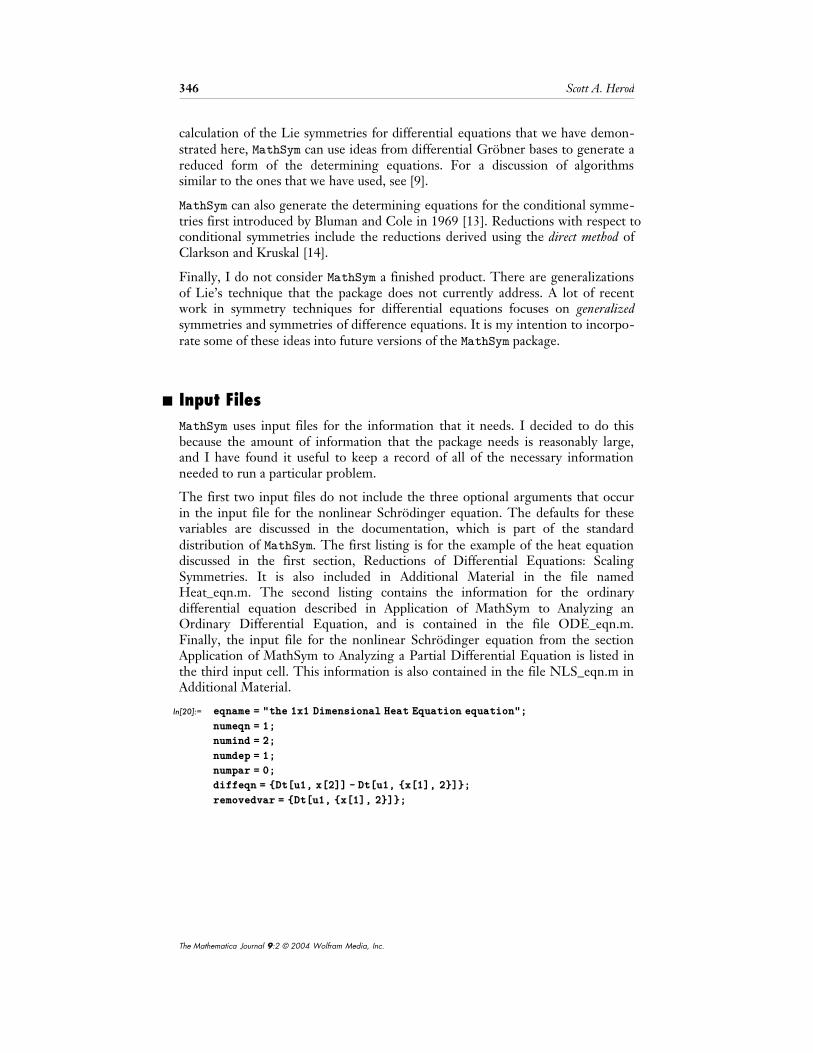
‡ Input FilesMathSym uses input files for the information that it needs. I decided to do thisbecause the amount of information that the package needs is reasonably large,and I have found it useful to keep a record of all of the necessary informationneeded to run a particular problem.

The first two input files do not include the three optional arguments that occurin the input file for the nonlinear Schrödinger equation. The defaults for thesevariables are discussed in the documentation, which is part of the standarddistribution of MathSym. The first listing is for the example of the heat equationdiscussed in the first section, Reductions of Differential Equations: ScalingSymmetries. It is also included in Additional Material in the file namedHeat_eqn.m. The second listing contains the information for the ordinarydifferential equation described in Application of MathSym to Analyzing anOrdinary Differential Equation, and is contained in the file ODE_eqn.m.Finally, the input file for the nonlinear Schrödinger equation from the sectionApplication of MathSym to Analyzing a Partial Differential Equation is listed inthe third input cell. This information is also contained in the file NLS_eqn.m inAdditional Material.

In[20]:= eqname = "the 1x1 Dimensional Heat Equation equation";numeqn = 1;numind = 2;numdep = 1;numpar = 0;diffeqn = 8Dt@u1, x@2DD - Dt@u1, 8x@1D, 2<D<;removedvar = 8Dt@u1, 8x@1D, 2<D<;

346 Scott A. Herod


In[27]:= eqname = "a nonlinear ODE ";numeqn = 1;numind = 1;numdep = 1;numpar = 0;diffeqn = 8Dt@u1, x@1D, x@1DD + s@1D u1 Dt@u1, x@1DD + s@2D u1^3<;removedvar = 8Dt@u1, x@1D, x@1DD<;

In[34]:= eqname = "the Nonlinear Schroedinger equation";tech = "Classical";splitlist = True;sortstyle = "Lexicographical";numeqn = 2;numind = 2;numdep = 2;numpar = 0;diffeqn = 8Dt@u1, 8x@1D, 2<D - Dt@u2, x@2DD + 2 Hu1 * u1 + u2 * u2L * u1,

Dt@u2, 8x@1D, 2<D + Dt@u1, x@2DD + 2 Hu1 * u1 + u2 * u2L * u2<;removedvar = 8Dt@u1, 8x@1D, 2<D, Dt@u2, 8x@1D, 2<D<;

‡ AcknowledgmentsI wish to thank Willy Hereman and Elizabeth Mansfield for discussions ofcomputer techniques used when computing symmetries and Mark J. Ablowitzand Peter Clarkson for comments on the use of symmetries of differentialequations. Thanks to James H. Curry for reading and commenting on numerousversions of this manuscript. Finally, I wish to thank the staff at Wolfram Re-search, especially Alexei Bocharov, for help with the intricacies of Mathematica.

Supported in part by the Department of Energy under grant DOE DE-FG03-94ER25194.

‡ References[1] S. Lie, “Über die Integration durch bestimmte Integrale von einer Klasser linearer

partieller Differentualgleichungen,” Arch, for Math., VI, Heft 3, 1881 S. 328–368.

[2] F. Schwartz, “Symmetries of Differential Equations: From Sophus Lie to ComputerAlgebra,” Siam Review, 30, 1988 pp. 450–481.

[3] A. V. Bocharov, “Symbolic Solvers for Nonlinear Differential Equations,” The Mathemat-ica Journal, 3(2), 1993 pp. 63–69.

[4] G. W. Bluman and S. Kumei, Symmetries and Differential Equations, New York:Springer-Verlag, 1989.

[5] P. J. Olver, Applications of Lie Groups to Differential Equations, New York: Springer-Ver-lag, 1986.

[6] L. V. Ovsiannikov, Group Analysis of Differential Equations (W. F. Ames, ed.), NewYork: Academic Press, 1982.



[7] N. H. Ibragimov, Lie Group Analysis of Differential Equations, Boca Raton: CRC Press,1994.

[8] G. Helzer, "Grobner Bases,” The Mathematica Journal, 5(1), 1995 pp. 61–73.

[9] F. Schwartz, “An Algorithm for Determining the Size of Symmetry Groups,” Computing,49, 1992 pp. 95–115.

[10] S. A. Herod, “Families of Exact Solutions for the Barotropic Vorticity Equation,” PAMTechnical Report, 1995.

[11] M. J. Ablowitz and P. A. Clarkson, Solitons, Nonlinear Evolution Equations, and InverseScattering, Cambridge: Cambridge University Press, 1991.

[12] A. L. Rabenstein, Elementary Differential Equations with Linear Algebra, New York:Academic Press, 1975.

[13] G. W. Bluman and J. D. Cole, “The General Solution of the Heat Equation,” Journal ofMathematical Mechanics, 18(11), 1969 pp. 1025–1042.

[14] P. A. Clarkson and M. D. Kruskal, “New Similarity Solutions of the Boussinesq Equa-tion,” Journal of Mathematical Physics, 30, 1989 pp. 2201–2213.

‡ Additional MaterialMathSym11.m Heat_eqn.m ODE_eqn.m NLS_eqn.m Heat_run.nb NLS_run.nb READMEDocumentation.nb

Available at www.mathematica-journal.com.

About the AuthorScott A. Herod did postdoctoral research at the University of Colorado in Boulderwhere his interests included differential equations, dynamical systems, and computa-tional mathematics. He now works as a software consultant specializing in the videoindustry.

Scott A. HerodDepartment of Applied Mathematics University of Colorado, Boulder Campus Box 526 Boulder, Colorado 80309-0526 [email protected]

348 Scott A. Herod


Documents

Learning about Differential Equations from Their … Mathematica® Journal Learning about Differential Equations from Their Symmetries Scott A. Herod Symmetries form the basis of …