FINAL PROJECT REPORT - oead.at

FINAL PROJECT REPORT

KEF Project P196 MaMa-Hydro: Exploring Water Resources Planning and

Management options in the Nyangores Headwater Catchment of the Vulnerable Maasai Mara River Basin in Kenya

Volume I: Technical report

Authors:

Prof. DI Dr. Josef FürstA, Dr. Luke O. OlangB, Dr. Mathew HerrneggerA, Doris WimmerA, Paul OmongeB, Edgar KipkoechB

Institutions:

(A). Institut für Wasserwirtschaft, Hydrologie und Konstruktiven Wasserbau im Department für Wasser - Atmosphäre – Umwelt. Universität für Bodenkultur Wien – AUSTRIA

(B). Department of Water and Environmental Engineering, School of Engineering and Technology, Kenyatta University, Nairobi – KENYA

Funding:

Kommission für Entwicklungsforschung (KEF) im OeAD

Dezember 2015

Universität für Bodenkultur Wien University of Natural Resources and Life Sciences, Vienna

Department of Water, Atmosphere and Environment Institute of Water Management, Hydrology and Hydraulic Engineering

2

TABLE OF CONTENT 1 Introduction and objectives .......................................................................................... 3

1.1 Background and motivation......................................................................................... 3

1.2 Objectives .................................................................................................................... 4

1.3 A short narrative of the main project activities ........................................................... 4

1.4 Structure of the report ................................................................................................ 6

2 Assessment of the current status of water resources .................................................. 7

2.1 Development of a consistent geodatabase ................................................................. 7

2.1.1 Organisation of the datasets ................................................................................ 7

2.1.2 Common geographic reference ............................................................................ 8

2.1.3 Map template ....................................................................................................... 9

2.1.4 Datasets in the Geodatabase and Metadata catalogue ....................................... 9

2.2 Relevant information from previous work and open sources ................................... 13

2.2.1 Basin characteristics ........................................................................................... 13

2.2.2 Characterization of important datasets ............................................................. 24

2.3 Original data collected within the project ................................................................. 38

2.3.1 Field mapping of water sources and sinks ......................................................... 38

2.3.2 Consistent land cover maps to assess land cover change .................................. 46

3 Simulation of the water demand – supply relationship using WEAP .................... 57

3.1 Introduction and aims ................................................................................................ 57

3.2 WEAP Model .............................................................................................................. 58

3.3 Results ........................................................................................................................ 59

3.3.1 Study area ........................................................................................................... 59

3.3.2 WEAP Application ............................................................................................... 60

4 Capacity building ......................................................................................................... 69

4.1 GIS Training Workshop at Kenyatta University ......................................................... 69

4.2 Support of post graduate students within the project .............................................. 70

4.3 Stakeholder workshop in Bomet ............................................................................... 70

4.4 Equipment Purchase and Software Acquisition ........................................................ 71

4.5 Memorandum of understanding between BOKU and KU ......................................... 71

5 Summary and conclusions .......................................................................................... 73

6 References..................................................................................................................... 79

Introduction and objectives 3

1 Introduction and objectives

1.1 Background and motivation Many developing countries are today facing formidable freshwater planning and management challenges. Allocation of limited water resources, degradation of environmental quality and lack of appropriate policies for sustainable water management are key issues of increasing concern. In Kenya, only less than 65% of the population has access to safe drinking water. The country is largely considered as water scarce and still lagging behind in the realization of the Millennium Development Goals (MDG) related to provision of equitable and reliable water resources. It is for this reason that the Government of Kenya has more recently begun institutional reforms in the water and sanitation sector to provoke relevant research geared towards achievement of the MDG and Vision 2030 (FAO 2007; AMCOW 2010; MPND 2005; UNDP 2012).

Presently, the majority of water resources used for domestic purposes, agriculture and irrigation, and hydropower generation in Kenya comes from surface water systems. However, the water systems are facing significant environmental degradation consequent of inapt human practices and climate change and variability effects. Generally, studies that explore water resource planning options, by integrating the existing society needs, for purposes of sustainable planning and management are very few in Kenya. This is largely because many regions are faced with widespread water scarcity, and hence emphasis is still being placed on exploring alternative sources to improve the per-capita water supply. Consequently, very little attention has been paid to pertinent scientific procedures of protecting the vulnerable headwater catchments important for replenishing the existing surface water systems (Onyando et al 2005).

An important area that is today severely threatened by the impacts of environmental changes is the Transboundary Mara River Basin (MRB) shared between Kenya and Tanzania. The basin has an area of about 13500 km2 and is drained by the Mara River with a total length of about 395 km. The catchment transverses regions of diverse land-use practices, including the Napuiyapi swamp within the Mau Escarpment; open savannah grasslands for livestock pasture; small to large-scale agriculture; and the world famous Maasai Mara National Reserve amongst others. Recent evidence of the MRB however, already indicates significant deforestation of the Mau forests in the headwater regions, declining river discharges in the mid to downstream regions, human and animal conflicts related to competing water uses, and significant loss of biodiversity and potential agricultural lands due to soil degradation.

It is for such reasons that several organizations have, in the recent past, joined hands in attempts to restore the affected ecological and ecosystem services. Consequently, several initiatives including the Global Water for Sustainability (GLOWS) Program and WWF - Eastern and Southern Africa Regional Programme Office (WWF-ESARPO) with financial support from the United States Agency for International Development-East Africa (USAID-EA) (http://globalwaters.net) were started. The project, which ended in May 2012, largely assessed the reserve flows of the Mara River basin for purposes of capacity building and extended conservation management. Generally, the MRB in entirety is a very important ecological ecosystem that supports various socio-economic activities in the region.


Degradation of its river flows, for instance, poses a big threat to tourism through the Great Annual Wildebeest Migration considered today as a world heritage. The MRB therefore, requires comprehensive research that continually allows the application of new technologies important for ecosystems management and restoration.

In this study, we focus on the Nyangores headwaters sub-catchment, because ongoing land cover changes are very dynamic in this part and the effect of these changes extends on the whole downstream part of the MRB.

1.2 Objectives The main objective is to assess the hydrology and water demand-supply relationships in the upstream Nyangores headwater catchment of the MRB (N-MRB). To achieve this, the study pursued three specific objectives:

1 Assessment of the current status of water resources

Managing the water resources requires an understanding of the existing related practices in the region, based on comprehensive information on the physical and hydro-meteorological properties of the catchment. This objective therefore, involves the compilation of relevant information on topography, geology, soils, hydrology, land cover and land use, as well as capturing the present water use practices related to withdrawals, preferences for supply.

2 Simulate the Water Demand-Supply relationship using a water resource model

For future planning purposes, it is important to project the future status of the water resource situation. To achieve this, the WEAP model is used. Because the model is data intensive and provides many modelling capabilities, this study focuses on applications for planning and future management only based on the information from objective 1

3 Capacity Building for improved water resource management and enhancement of policy mainstreaming

From the study results, adaptation measures are derived and training needs identified for the concerned stakeholders in the region, especially on the possible management strategies. Because the department of WEEN at Kenyatta University still lacks sufficient human resource capacity, we supported and trained postgraduate students, while fortifying the need for future exchange of students between the two Universities.

1.3 A short narrative of the main project activities The MaMa-Hydro Project commenced officially in January 2014 with the transfer of funds to Kenyatta University by BOKU University. A brief description of the project details was consequently presented to the Vice Chancellor/Rector of Kenyatta University (KU) for validation of the project to allow use of the funds by the School of Engineering and Technology, according to the KU regulations.

To allow for the project commencement in the Nyangores sub catchment, a start-up expert visit to the catchment in Bomet County was organized between the 13th and 15th of February 2014. The aims of the visit were to meet the local administrative policy makers involved in water management in the area and allow for community participation in identifying the local water needs related to the project objectives. The experts involved BOKU and Kenyatta University experts of the project. The local stakeholders met during the visit included the local Water Resource User Association (WRUA) representatives of the


Nyangores River, the Bomet County authorities in the Ministry of Water, Environment and Natural Resources for policy support and meeting local women water users for understanding their water challenges in the basin. In outline, the visit was important in understanding the requirement for an inventory of the water sources, sinks, data status and related water issues that can be addressed by the study.

One of the activities of the MaMa-Hydro project was to carry out an expert training workshop on GIS based water resource modeling and management. Consequently, a training workshop on “Application of GIS in Water Resources Management” was arranged at Kenyatta University from the 17th – 21st of February 2014. The workshop was attended by regional stakeholders from East Africa concerned with applying novel geo-spatial technologies in understanding and protecting the vulnerable river basins in the region. Proficient presentations on exploring new spatial and hydrological tools towards catchment management and pertinent decision support were made by regional experts on the first day. The remaining part of the time was spent on lectures and hands-on work carried out largely by BOKU University staff with the support of data provided by Kenyatta University and ESRI – Kenya. The topics in the GIS training section particularly emphasized techniques and skills required by students and young staff who then contributed to the MaMa-Hydro project). Two of the participants successfully applied to be supported in their master thesis.

The data required to achieve the objectives of the project include existing data to be collected from various sources as well as original information to be collected and/or measured in the field. A major deficit in the existing information base so far relates to data on water sources, their capacities, type and usage.

A first field work campaign was undertaken for a period of 20 days in June 2014 by two master students, under advisory of Dr. Olang. The first week was not very successful due to the heavy rains in the region rendering some parts inaccessible. Consequently, the week was largely spent on gathering literature within the WRUA and regional water resources county offices. During this time, the available hydro-meteorological datasets were acquired by Mr Ngeno. Despite the bad weather, this visit managed to acquire a good number of the datasets for the study.

A total of 52 locations where water is accessed for various uses were approached to record information considered to be relevant for water management. Besides of the co-ordinates and elevation, physical properties were measured – electrical conductivity, temperature and discharge (at springs). Electrical conductivity is thereby loosely related to water quality. Discharge is primary information for the availability of water, although a single snapshot measurement cannot inform about the temporal variability. It is not affordable in the framework of this project to establish permanent discharge gauges at the springs but at least a few additional measurements at selected springs are envisaged. Additionally, a short characterization of the site, whether it is a protected or unprotected spring, and a verbal semi-quantitative description of the use and users have been recorded.

In May, 2014, the MaMa-Hydro project team was invited to present the work in Austrian TV under the banner “Mother Earth”. This effort provided the opportunity to consolidate and disseminate our efforts in a bid to save the vulnerable Mara River basin presently being threatened by environmental degradation. Details of this presentation can be found in the KEF website titled: KEF-Projekt 196 MaMa-Hydro im ORF-TV (Wien Heute).

Activities since autumn 2014 included further field work to extend information on water


supply and demand. Involved MSc students were trained in the use of the WEAP model, enabling them to apply WEAP to the Nyangores.

On September 9th, 2015 the preliminary results of the projected were presented to and discussed with the local stakeholders in a workshop in Bomet, the administrative center of the county. The workshop was attended by high ranked representatives of the county government and water management organisations WARMA and WRUA, including the Minister for Public Health and Environment.

1.4 Structure of the report The complete project report has been compiled in 3 volumes: Volume I (this volume) is the technical report which follows closely the outline of the proposal, organized by the specific objectives as listed above. Volume II is compiled as a book of maps in DIN A3 format. Volume III is the detailed financial report.

Chapter 2 documents the current status of water resources in the Nyangores watershed. The first major sub-chapter is a summary and compilation of relevant information from previous work and open sources. In the second part, original data collected in the context of MaMa-Hydro are presented and summarized.

Chapter 3 presents the WEAP based simulation studies of the water demand – supply relationship, including scenario simulations of possible future developments.

Chapter 4 reports the achievements in capacity building and policy mainstreaming for water resource management.

Assessment of the current status of water resources 7

2 Assessment of the current status of water resources Both, the Mara River basin as a whole, as well as the Nyangores sub-basin, have been subject to various research projects related to water resources and their management in the past. To avoid unnecessary redundancies, we did a comprehensive research on these sources and extracted the relevant information. Emphasis was laid especially on the collection of spatial datasets which were transformed into a common spatial reference, documented in a standard format and added to a conveniently usable geodatabase (2.1). From the most important spatial datasets, maps were created in a common layout and provided in a book of maps (see Volume II of this report). A summary of this information is provided in sections 2.2 (previous work and open sources) and 2.3 (new datasets created within the project).

2.1 Development of a consistent geodatabase

2.1.1 Organisation of the datasets

The amount of information in the database is dominated by publicly accessible information from various sources, but also the spatial datasets created within the project are included.

Datasets in a geodatabase can be organised by different criteria: by topic, methodical-technical properties, resolution of the model or spatial reference amongst others (Hake et al. 2002).

Figure 1: Organisation of the datasets arranged by type and data format *analogue maps, which have been added to the database as images in raster format

The schematic in Figure 1 shows a classification of the data regarding methodical-technical criteria. One criterion was the data format (vector or raster), the other one was the structure of the data. The format of the data can be easily assigned, but often vector data has


originated from raster data: for example stream networks and catchments have been derived from a Digital Elevation Model by calculating the flow direction and flow accumulation for every pixel. Cells with a high flow accumulation to their cell can be used to identify stream networks, which are converted into vector format; furthermore every dataset derived from a satellite image is derived from a raster dataset. For example the Globcover dataset is a vector dataset directly converted from a raster.

Spatial resolution and spatial extent do often go along: For a dataset with a wide spatial extent, a high spatial resolution is usually not required and thus too expensive. For example, it will never be reasonable to create a geological map of the whole African continent with the same level of detail required for a map of the small Nyangores River basin. Especially for vector data the spatial resolution is not easy to reproduce. On the other hand the pixel size of a raster dataset makes it easy to find out the spatial resolution of the model. Concerning the spatial aspect, the data in the geodatabase can be subdivided into classes of different spatial scales: the dataset contains data (1) of the whole African continent, (2) of the republic of Kenya or (3) just of the Mara- or Nyangores basin. In our case, a classification using this aspect is not reasonable, because the focus of the project lies in the Nyangores River basin.

To keep navigation easy within the database and for direct comparison, the data was arranged by thematic issues. The same arrangement has also been used for the subsequent discourse of used datasets.

2.1.2 Common geographic reference

The spatial datasets were originally available in different geographic reference systems. Although GIS can handle data sources with different coordinate systems, it is more efficient to set up a common geographic reference and coordinate system for all data.

For Kenya, the most suitable system is UTM Zone 36S, based on the WGS 1984 datum (Table 1).

Table 1: Used spatial reference system

WGS 1984 UTM Zone 36S Projection Transverse Mercator Datum WGS 1984 False Easting 500 000.00 False Northing 10 000 000.00 Central Meridian 33.00 Scale Factor 0.9996 Latitude Of Origin 0.00 Units Meter


2.1.3 Map template

To support convenient and consistent reading of the maps and to facilitate also comparison between them, a standardized layout was created (Figure 2), including

• Title centered above main map frame • Overview map • Legend • Description, explaining map information, coordinate system and project context • Main map frame.

Figure 2: Standard layout used for the maps

2.1.4 Datasets in the Geodatabase and Metadata catalogue

Table 2 gives an overview of the dataset collected within the MaMa-Hydro Project and which are included the Geodatabase. This datasets cover different thematic areas, namely

• Hydrology

• Towns

• Borders

• Others

• Topography

• Soils


• Landcover

• Satellite images (Landsat)

• Geology and

• Geomorphology.

Table 2: List of the datasets contained in the Geodatabase Thematic area / Dataset Name Description Extent Type Format Year

publish. Resolution Scale

Author/ Publisher

HYDROLOGY

Mara_MonitoringStations Mara River Basin Monitoring Stations

Upper Mara

point Vector Florida International University

Kenya_RainfallStations Rainfall Stations Kenya point Vector Kenya Meteorological Service

Africa_Waterbodies Inland water bodies in Africa

Africa area Vector 2000 1:1000000 FAO - AQUASTAT

Mara_Wetland Mara River Basin Waterbodies Digitized from Landsat ETM imagery

Mara area Vector Florida International University

Mara_Stream STREAM Mara line Vector 2014 90x90 Mara_StreamDetail100 Mara line Vector 90x90 Mara_Watershed WATERSHED Mara area Vector 2014 90x90 Nyangores_Watershed Nyangores area Vector 2014 90x90 Nyangores_PointsFieldTrip FIELDTRIP_SPRING

S Nyangores point Vector 2014

TOWNS Tanzania_MajorTowns Towns of Tanzania

- AFRICOVER Tanzania point Vector 2002 1:100000 FAO -

Africover Tanzania_OtherTowns Tanzania point Vector 2002 1:100000 Kenya_MajorTowns Towns of Kenya -

AFRICOVER Kenya point Vector 2002 1:100000 FAO -

Africover Kenya_OtherTowns Kenya point Vector 2002 1:100000 Mara_Towns Location of Towns

and Villages in the Mara River Basin, Africa

Upper Mara

point Vector Florida International University

BORDERS

Africa_Boundaries African Boundaries Kenya area Vector USGS Kenya_Provinces Provinces Kenya area Vector David

Muthami on ArcGIS.com

Kenya_Counties The 47 Counties of Kenya

Kenya area Vector David Muthami on ArcGIS.com

Kenya_Districts The 71 Districts of Kenya


Kenya_Constituencies Constituencies of Kenya (2002)


Kenya_Divisions Divisions of Kenya Kenya area Vector David Muthami on ArcGIS.com

OTHERS

Kenya_Roads Road_All Kenya line Vector David Muthami auf ArcGIS.com

TOPOGRAPHY DEM_3arcseconds SRTM 3 Arc- Mara area Raster 2014 90x90 SRTM


Thematic area / Dataset Name Description Extent Type Format Year publish.

Resolution Scale

Author/ Publisher

Seconds DEM_1arcsecond SRTM 1 Arc-Second

Global Mara area Raster 2014 30x30 SRTM

SLOPE Derived from SRTM 1 Arc-Second Global

Mara area Raster 2014 30x30 SRTM

SOILS

Soil_1_KenyaAtlas_1969 National Atlas of Kenya - Soil

Kenya area Analog 1969 1:3000000 Gethin-Jones, G.H., Scott, R.M., E.A.A.F.R.O.; Survey of Kenya 1969

Soil_2_AfricaSoilMap_2006 Major Soils for Africa

Africa area Vector 2006 1:5000000 FAO

Soil_3_KenyaSOTER_2007 Soil and Terrain database for Kenya (SOTER)

Kenya area Vector 2007 1:1000000 ISRIC, Kenya Soil Survey

Soil_4_AfricaSoilAtlas_2014 Soil Atlas of Africa Africa area Vector 2014 1:3000000 ISRIC LANDCOVER

Landcover_1_vegetation_1969 Climate and Vegetation. Sheet 1. D.O.S.(L.R.) 3059.

Nyangores area Analog 1969 1:250000 Trapnell, C.G./British Government, Directorate of Overseas Surveys and Kenya Government

Landcover_2_AfricoverKenya_2002 Multipurpose landcover database for Kenya - Africover

Kenya area Vector 2002 1:200000 FAO

Landcover_3_AfricaRaster_2004 GLC-2000 Based 1 km Global Land Cover - Africa

Africa area Raster 2004 1000x1000 FAO

Landcover_4_AfricoverKenya_2007 Aggregated land cover database for Kenya (Africover) for tsetse habitat mapping

Kenya area Vector 2007 1:200000 FAO

Landcover_5_Globcover_2009 Land cover of Kenya - Globcover Regional

Kenya area Vector 2009 300x300 FAO/ISRIC

Landcover_6_MaraReferencePoints

Reference Points for land cover classification

Mara point Vector ? GIS FIU EDU

Landcover_7_MaMaHydro_1995 Land cover of Nyangores 1995

Nyangores area Vector 2015 30x30 E. Ngeno, KU

Landcover_8_ MaMaHydro_2010 Land cover of Nyangores 2010

Nyangores area Vector 2015 30x30 E. Ngeno, KU

Landsat

Landsat_1973 Landsat 1-5 MSS 1973

Mara area Raster 1973 60x60

Landsat_1986 Landsat 4-5 TM 1986

Nyangores area Raster 1986 30x30

Landsat_1995 Landsat 4-5 TM 1995


Landsat_2000 Landsat 7 ETM+ 2000


Landsat_2010 Landsat 7 TM 2010 Nyangores area Raster 2010 30x30 Landsat_2014 Landsat 8 OLI/TIRS

2014 Nyangores area Raster 2014 30x30


Thematic area / Dataset Name Description Extent Type Format Year publish.

Resolution Scale

Author/ Publisher

GEOLOGY

Africa_Geology National Atlas of Kenya: Geological Map

Africa area Analog 1962 1:3000000

GEOMORPHOLOGY

Kenya_Geomorphology Geomorphology - Landform and Lithology for Kenya - Africover

Kenya area Vector 2003 1:350000 Survey of Kenya

Geodatabases – like all data collections – need a certain amount of metadata to enable proper use by users apart from the creators of the datasets. Therefore, a metadata catalogue was compiled with a reasonable amount of attributes for the basic understanding of the dataset. The catalogue is similar to the ArcGIS metadata style. The metadata catalogue only takes into account information about geographical datasets in GIS. Exemplarily, the metadata catalogue for the “Mara_Stream” file is shown Table 3.

Table 3: Example of metadata record for the Geodatabase Feature Class "Mara_Stream"

title Mara_Stream

distribution format Personal GeoDatabase Feature Class

item description

abstract/summary Synthetic stream network of the Mara River

description Data derived from a Digital Elevation modell with a resolution of 90x90 metres using ArcHydroTools

usage

keywords Mara River, Hydrology, Stream Network, ArcHydroTools

extent

geographic extent

West longitude 33.934699

East longitude 35.782959

North latitude -0.470051

South latitude -1.867392

extent in the item's coordinate system

West longitude 604009.728400

East longitude 809633.018131

South latitude 9793568.721886

North latitude 9947983.502186

resolution (optional for raster data)

Data derived from a Raster with a resolution of 90x90 metres

spatial reference

geographic coordinate system GCS_WGS_1984

projected coordinate system WGS_1984_UTM_Zone_36S

projected coordinate reference details

For detailed information look in ArcGIS

geometry type Polyline

time reference


time reference of basis data Digital Elevation Model from 2008

date of publication 2015

processing status complete

maintenance/update frequency no updates intended

name/contact of originator/editor Wimmer Doris, University of Natural Resources and Life Sciences, Vienna

data source DEM from http://dwtkns.com/srtm/

use limitation no limitations

attributes

alias OBJECTID

data type OID

description Sequential unique integer numbers that are automatically generated.

alias Shape

data type Geometry

description Coordinates defining the features.

Some metadata about purely technical properties that are generated automatically by running a tool in ArcGIS are not listed in the metadata catalogue above.

2.2 Relevant information from previous work and open sources

2.2.1 Basin characteristics

2.2.1.1 Location

The river Nyangores originates in the Southwest of Kenya in the Keringet area (Kiragu 2009) situated in the Mau forest, the largest remaining forest in Kenya (Minaya et al. 2013) and one of the largest indigenous moist forests in East Africa (Okeyo-Owuor 2007). The area around Kiptunga forest with Enapuiyapui swamp (Mango 2010) in Southern Rift Valley Province (Terer 2005) in Nakuru County (MRWUA 2011) is drained by several tributaries that form the Nyangores River – those are namely: Ainopngetunyek, Chepkositonik, Kagawet, Kapsabet and Kiprurugit River (Terer 2005). The Nyangores runs over a distance of 94 km in southwest direction through the Counties Nakuru, Narok and Bomet before joining Amala River at Kaboson to form the main Mara River (MRWUA 2011). Nyangores and Amala River are the two main perennial tributaries of the Mara River, which is lifeline for the people, for livestock, wildlife and for the whole ecosystem of the Maasai Mara on the Kenyan and the Serengeti national park on the Tanzanian side. On its way through the Maasai Mara the Mara River is joined by Talek, Engare Engito and Sand River. The main tributary on Tanzanian side is the Bologonja River. After leaving the protected areas, the 395 km long Mara River flows through the Mosirori Swamp (Mango 2010), where it provides water and nutrients for the vast wetlands. At Musoma the river finally drains into Lake Victoria, where it serves as one of the headwaters of the Nile Basin (Kiragu 2009).

Richard et al. (2014) quotes the geographic extent of the Mara River Basin as follows: Latitudes from 0° 19‘ S to 1° 58‘ S and longitudes between 33° 53‘ E and 35° 54‘ E. The Nyangores River Basin is located between latitudes 0° 22’ and 1° 02’ south of the equator and longitudes 35° 12’ and 35° 47’ E.

The catchment area delineated in GIS covers an area of 933 km². Throughout the literature


the given size of the catchment area refers to the catchment area at the river gauge LA03 at Bomet. This might be useful for hydrological models, because runoff data is available for this point. At this gauge the catchment area is 693 km².

Figure 3: Location of the Nyangores River Basin (red)

The highest points of the Mara River Basin are situated in the Mau-Escarpments at an altitude of 3063 m a.s.l. in the Mara and 2970 m a.s.l. in the Nyangores River Basin. The confluence of Nyangores and Amala River is at an altitude of 1695 m a.s.l. from where the river falls gradually, ending at an altitude of 1128 m a.s.l. at the basin outlet of Mara River into Lake Victoria.


Table 4: Overview of characteristic information about the Nyangores River Basin

Coordinates Longitude 35° 12' E - 35° 47' E

Latitude 00° 22' S - 01° 02' S

Catchment area Drainage area at Bomet LA03 693 km²

Drainage area at Kaboson 933 km²

Elevation Highest Point 2970 m a.s.l.

River gauge LA03 at Bomet 1900 m a.s.l.

Basin outlet at Kaboson 1695 m a.s.l.

2.2.1.2 Topography

The Mau forest is located 200 km southwest of Nairobi in the montane rain forest region. It covers an area of about 900 km² and is one of the largest remaining moist forests in East Africa. Mau forest poses an important area for water accumulation not only for the Mara River, but also for Sondu and Ewaso Ngiro rivers (Okeyo-Owuor 2007). The tributaries, that feed the Nyangores and subsequently the Mara River originate in the Transmara forest, which is an extension of the Mau-Complex to the east (Terer 2005).

The hills of the Rift Valley with their highest points in the Mau-escarpments, where the Nyangores River Basin is situated, are a result of the uplifting activities in the area. The highest regions – like Tiroto, Masare Kyogong and the Motigo hills – show a steep, deeply dissected relief, that has been eroded by water. To the south the steep escarpments turn into gentle hills, gradually flattening between Sigor and Kaboson (Mbuvi and Njeru 1977; Terer 2005). The hilly catchment has got 50% of its total area above an altitude of 2200 m a.s.l and a high precipitation (MRWUA 2011). After the confluence of the Nyangores and the Amala River the combined Mara River flows at a gentler gradient through wooded grasslands, the Maasai Mara Rerservat, the Serengeti and along the vast plain of the Mosirori Swamps into Lake Victoria (Kiragu 2009).

2.2.1.3 Geology

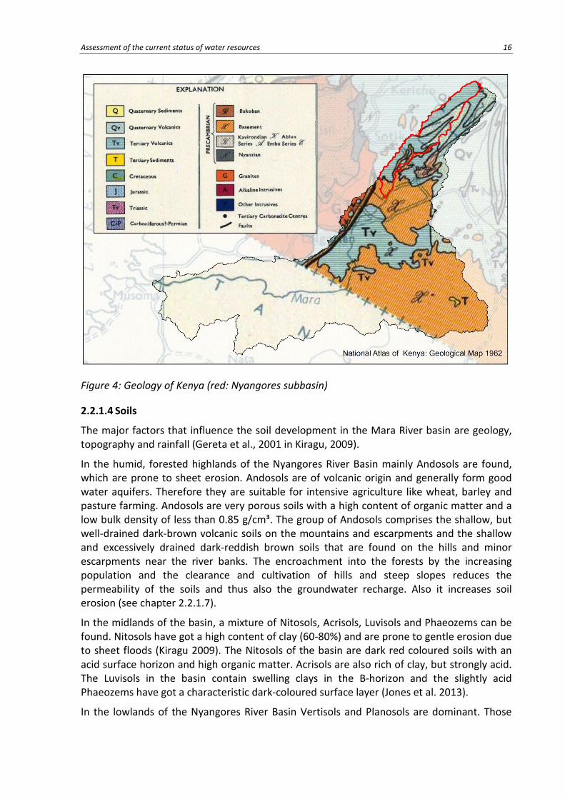
The majority of the area consists of poorly consolidated, pyroclastic material like volcanic tuffs and ashes, that alter into clay and frequently are overlain by volcanic ashes (Mbuvi and Njeru 1977). In large parts of the river basin those quarternary and tertiary Volcanics of the Rift valley are dominant, while around Kaboson the Precambrian bedrock consisting of Kavirondian sediments, emerges (Figure 4). Petrographical analyses of the Kavirondian sediments occurring in western Kenya showed that the sediment was derived from old granite rocks, volcanic rocks and recycled sedimentary rocks (Ngecu 1991).


Figure 4: Geology of Kenya (red: Nyangores subbasin)

2.2.1.4 Soils

The major factors that influence the soil development in the Mara River basin are geology, topography and rainfall (Gereta et al., 2001 in Kiragu, 2009).

In the humid, forested highlands of the Nyangores River Basin mainly Andosols are found, which are prone to sheet erosion. Andosols are of volcanic origin and generally form good water aquifers. Therefore they are suitable for intensive agriculture like wheat, barley and pasture farming. Andosols are very porous soils with a high content of organic matter and a low bulk density of less than 0.85 g/cm³. The group of Andosols comprises the shallow, but well-drained dark-brown volcanic soils on the mountains and escarpments and the shallow and excessively drained dark-reddish brown soils that are found on the hills and minor escarpments near the river banks. The encroachment into the forests by the increasing population and the clearance and cultivation of hills and steep slopes reduces the permeability of the soils and thus also the groundwater recharge. Also it increases soil erosion (see chapter 2.2.1.7).

In the midlands of the basin, a mixture of Nitosols, Acrisols, Luvisols and Phaeozems can be found. Nitosols have got a high content of clay (60-80%) and are prone to gentle erosion due to sheet floods (Kiragu 2009). The Nitosols of the basin are dark red coloured soils with an acid surface horizon and high organic matter. Acrisols are also rich of clay, but strongly acid. The Luvisols in the basin contain swelling clays in the B-horizon and the slightly acid Phaeozems have got a characteristic dark-coloured surface layer (Jones et al. 2013).

In the lowlands of the Nyangores River Basin Vertisols and Planosols are dominant. Those


soils are quite common in the rest of the Mara Basin too. Vertisols are imperfectly drained, dark grey/brown soils, developed on granites, also containing swelling clay. The dark grey/brown Planosols consist of very firm clay and have got an influence of volcanic ash (Terer 2005).

The previous list of soils found in the basin refers to the classification of soils of the FAO. For example the soil map from 1969 uses a different classification and nomenclature for soils. Still, both of them show: The red and brown soils are well drained and mostly of volcanic origin, while the soils in the south are often alluvial deposits, which are less porous and imperfectly drained.

2.2.1.5 Hydrology

General Information

The most important hydrological processes are precipitation, evapotranspiration, water infiltration and surface runoff. Infiltration is mainly influenced by soil characteristics, surface, vegetation and variables like rainfall amount and intensity (Terer 2005). An intact water cycle should provide good water quality for communities, agricultural activities, tourist facilities and mining activities. In addition to that, it has to provide habitats for fish, plants, people and wildlife in the basin. Those diverse demands are sometimes hard to combine, what makes the Mara basin vulnerable to erosion (Kiragu, 2009 after Mati et al., 2008).

Climate and Rainfall

Characteristic for the basin is the tropical dry/wet dry climate that changes greatly with the change in altitude. The location within the Inter-Tropical Convergence Zone (ITCZ) is responsible for the seasonal variation in rainfall. Seasons are bimodal, with the long rains between March and June, caused by the Southeast Trade winds and calming down after the storms brought by the Southwest Trade winds. The short rains are experienced in November and December. The north-easterly winds coming from the Sahara Desert bring the dry seasons (Kiragu 2009; Krhoda 2005; Terer 2005).

Rainfall data is recorded by the Kenya Meteorological Department, WRMA and private operators (MRWUA 2011).

According to information provided by the Kenya Meteorological Department, there are eight operating rainfall stations spread over the Nyangores basin (Table 5).


Table 5: Rainfall Stations in the Nyangores sub-catchment

STATION NAME STATION NUMBER YEAR OPENED OPERATING TIME

SOTIK,KABOSON GOSPEL MISSION 9135008 1958 57 years

BOMET DISTRICT OFFICE 9035227 1958 57 years

BOMET WATER SUPPLY 9035265 1966 49 years

MERIGI CHIEF'S CENTRE 9035312 1981 34 years

SOTIK, TENWIK MISSION 9035079 1939 76 years

NYANGORES FOREST STATION 9035302 1979 36 years

KARINGET FOREST STATION 9035324 1984 31 years

ELBURGON,BARAGET FOREST STATION 9035241 1961 54 years

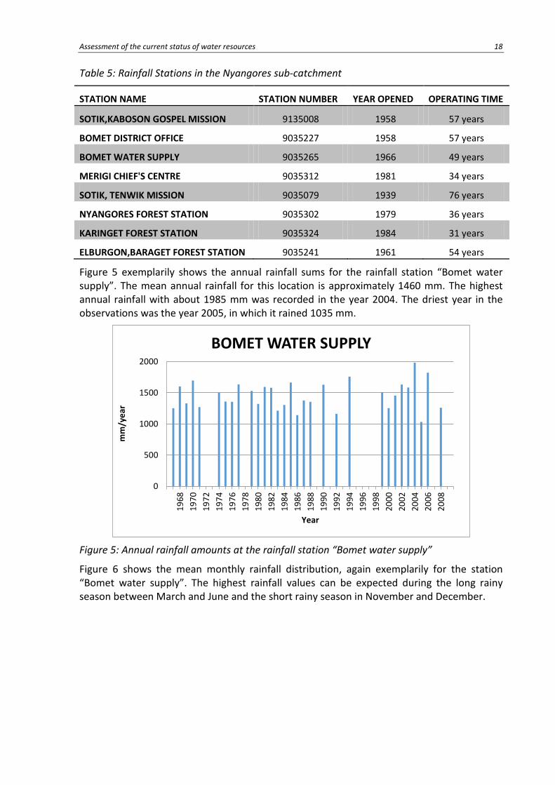
Figure 5 exemplarily shows the annual rainfall sums for the rainfall station “Bomet water supply”. The mean annual rainfall for this location is approximately 1460 mm. The highest annual rainfall with about 1985 mm was recorded in the year 2004. The driest year in the observations was the year 2005, in which it rained 1035 mm.

0

500

1000

1500

2000

1968

1970

1972

1974

1976

1978

1980

1982

1984

1986

1988

1990

1992

1994

1996

1998

2000

2002

2004

2006

2008

mm

/yea

r

Year

BOMET WATER SUPPLY

Figure 5: Annual rainfall amounts at the rainfall station “Bomet water supply”

Figure 6 shows the mean monthly rainfall distribution, again exemplarily for the station “Bomet water supply”. The highest rainfall values can be expected during the long rainy season between March and June and the short rainy season in November and December.


0

50

100

150

200

250

300

1 2 3 4 5 6 7 8 9 10 11 12

mm

/mon

th

Month

BOMET WATER SUPPLY

Figure 6: Long-term mean monthly rainfall at the rainfall station “Bomet water supply”

The Mau Escarpment receives mean annual rainfall between 1000 and 1750 mm (Mati et al. 2005; Melesse et al. 2012). Mean annual rainfall decreases with falling altitude to 900 mm at Kaboson (Terer 2005) and 600 mm at Musoma (Kiragu 2009). Despite of an increasing trend in rainfall since 1959 (until 2003), inhabitants of the area reported a slightly decreasing rainfall trend in the catchment. An analysis of the rainfall data of the ten year period 1994-2003 confirmed that rainfall has started to increase, but also the frequency of extreme weather events like droughts and floods has increased (Terer 2005).

Temperature

Temperature depends, like rainfall, on the altitude and is 25°C in average for the Mara basin (Kiragu 2009). In Kaboson the mean annual temperature decreases to 19.8°C and around the edge of the forest it only is 17.6°C (Terer 2005). Water temperature varies from 12°C to 21°C (data collected from February to May) on forested, farmland and rangeland sites. The mean temperature in the forested area was 17.9°C and the farm- and rangelands hat a temperature of slightly above 19°C (Mbao et al. 2013).

Evapotranspiration

The long-term average potential Evapotranspiration (PET) was estimated with the Priestly-Taylor method and a temperature series from Kericho to be 1490 mm/year. Thus, rainfall and PET are in approximate balance in the Nyangores basin (Juston et al. 2014).

River discharge

The only river gauging station RGS 1LA03 is located 20 m upstream of the Bomet bridge, where the river drains an area of 693 km². The station has got three staff gauges and an artificial, rectangular weir, that impounds the river for the purpose of water abstraction for water supply of Bomet town (MRWUA 2011).

In general, quite high mean monthly discharges occur in the months from May to September as can be seen from the time series in Table 6 by (Krhoda 2005).


Table 6: Average monthly discharge from 1964 until 1992

RGS J F M A M J J A S O N D

1LA3 3,06 3,01 2,83 7,16 11,9 10,6 10,9 11,9 13,2 9,34 5,83 4,83

0

2

4

6

8

10

12

14

J F M A M J J A S O N D

Disc

harg

e [m

³/s]

Average monthly discharge 1964-1992

Figure 7: Hydrograph of the average monthly discharge from 1964 until 1992

The flow regime seems to be fairly balanced with a dry season in spring. Floods occur from April to September and during November and December as a result of the rainy seasons. The last devastating drought was 1999/2000 as a result of El Nino (Krhoda 2005). As a result of human activities – especially destruction of the forest, there has been a decrease in normal streamflow and a depletion of springs on the one hand, but an increased flood flow on the other hand (Terer 2005).

2.2.1.6 Water use and collection

There are several boreholes in the basin located and four dams used for water abstraction in Tenwek, Chengaina, Cheboin and Kaboson. From the about 1500 springs existing in the basin, 23 have been protected by WWF and a few more by Bomet municipality. Large parts of water for domestic use and farming comes from unprotected springs (MRWUA 2011) or the river itself (Terer 2005). In addition to domestic use and sanitation, the water resources are also important for agricultural purposes, like watering of livestock or large scale irrigation of agricultural land (Mango 2010; Minaya 2010). The demand of water for domestic use and agriculture increases due to population growth in the area (Mango 2010). Additionally water resources are important for the Nyangores and subsequently also for the Mara River for sustaining the plants and wildlife of the natural reserves of the Maasai Mara and the Serengeti.

2.2.1.7 Sediment budget

Erosion and Sedimentation are the main processes determining the sediment budget.


Erosion is influenced by rainfall intensity, land cover, slope and several soil characteristics including content of organic matter and microstructure. Especially in developing countries erosion is often caused by mismanagement in agriculture and forest clearance (Maniak 2005). The loss of vegetation and the agricultural cultivation lead to soil compaction, which decreases infiltration and thus leads to increased flood peaks caused by increased direct runoff of the rainfall. Also it leads to a reduction in groundwater regeneration that should replenish water bodies (especially during the dry season). Linked to the increasing flood peaks and the loss of land cover, sedimentation is increasing in the Nyangores basin (Terer 2005). In the northern parts of the basin, the occurrence of the easily eroded Andosols combined with the clearing of the forest, the intensive agriculture and the steep slope, cause a high loss of soil of the already thin layer. These developments lead to a soil deterioration in the headwaters of the catchment and diminishes the river’s ability to continue providing year-round flow. The upper wetlands are shrinking, while the lower wetlands in the Mosirori swamps have expanded by 387 % from 1973 to 2000 (Kiragu, 2009 after Mati et al. 2008). Further impacts of the increasing sediment load in the river are pollution of the Lake Victoria and the reduction in light penetration in the water column, that might reduce photosynthetic activity (Kiragu 2009). Soil resources could be preserved by terracing the steep, cultivated area. This has already been done during the colonial era, but has been slowly destroyed after independence (Terer 2005).

2.2.1.8 Water quality

The „Nyangores River Subcatchment Management Plan“ differentiates between point and non-point sources of pollution (MRWUA 2011; Kilonzo et al. 2014):

Point sources are:

• Municipal Wastewater of the fast growing urban centres

• Domestic Wastewater

• Cattle watering tanks near the river banks

• Slaughter houses

• Car washing

• Solid Waste disposal along streets and markets

Non-point sources are mainly caused by inappropriate land use and are:

• Small scale farming, caused by misuse of agro-chemicals, farming and irrigating on steep slopes

• Overgrazing (in the lower Nyangores basin)

• Deforestation of Mau-forest and erosion of the exposed area

• Urban storm runoff

• Washing and Bathing in the river

The water quality near the river’s source at Kiptagich is good but deteriorates on its way downstream due to human activities. To improve water quality, actions including construction of sanitation facilities or information of the population concerning proper agricultural practices, would be necessary. Additionally it would be good to carry out


continuous pollution monitoring (Richard et al. 2014), what is currently conducted on a quarterly basis at the RGS LA03. Physical, chemical and biological parameters are being measured (MRWUA 2011).

2.2.1.9 Climate change

The climate system affects all aspects of the hydrological cycle. Therefore the impacts of climate change have to be taken into account and have to enter the hydrological model in form of different scenarios. Future global warming and resulting higher temperatures would increase evaporation and thus alter soil moisture and infiltration (Mango 2010).

2.2.1.10 Flora

The area between 2300 and 2500 m above sea level is rich in indigenous flora and fauna (Okeyo-Owuor 2007). In other parts of the catchment land use changes caused by intensified human activities have severe impacts on the ecology of the basin (MRWUA 2011).

On the highlands, deciduous trees can be found, becoming up to 26 m high, while on the lowlands the vegetation is a mixture of wood-, bush- and grasslands. The dominant types of grass are the red oat grass (Themeda triandra) and the wiregrass (Pennisetum schimperi); the latter is common in overgrazed areas. The woodlands are dominated by acacia and Spiny camiphora species, while the fast growing, exotic eucalyptus trees can be found along the river bank. The high water demand of eucalyptus trees poses a problem especially in the dry seasons, where they exacerbate water scarcity (Kiragu 2009).

2.2.1.11 Fauna

The clear waters in the upper, forested part of the basin offer perfect conditions for primary production. A wide range of macroinvertebrates can be found her in some sites. For them the Mara Forest plays an important role in the supply of organic matter (MRWUA 2011). Increased sediment load in the lower parts might reduce primary production and therefor affect macroinvertebrates and fish. With an increase in nitrogen and phosphorus levels, dissolved oxygen might be reduced, what would have negative impacts on aquatic organisms too. The waterfall and the dam in Tenwek acts as a natural barrier for fish movement, what has a high impact on the biodiversity: Downstream the waterfall there can be found fish of the fish species Barbus, Labeo, Clarias and Mormyrus, while upstream only the fish species Clarias liocephalus has been recorded (MRWUA 2011). This species is abundant in the upper parts of the river, but is largely absent in the waters downstream, because it requires the water to have temperatures less than 18 °C and prefers a good water quality with a high content of dissolved oxygen (MRWUA 2011; Tamatamah 2009). The intensive cultivation of the basin does not only have an impact on flora and fauna on land, but also influences the ecology of the river and should therefore be planned with caution (Minaya 2010).

2.2.1.12 Population

The whole Mara basin is home to 1.1 million people, 775 000 of them living in Kenya. According to the 2009 Census, the population of the Nyangores basin is about 300 000 people (MRWUA 2011). With an annual population growth of 3 to 6% (Kiragu 2009) by the year of 2015 350 000 people are estimated to live in the basin (+3%). The largest city along Nyangores River is Bomet, with 95 000 inhabitants (Kilonzo et al. 2014) and the Bomet Central division has got the highest population density of the area with 388 persons per km²


(Terer 2005). In the last few years urban centers including Mulot, Olenguruone, Silibwet and Sigor have experienced rapid population growth. While the high-rainfall regions in the north have experienced population growth too, people are out-migrating of the lower, less productive areas of the basin (Kilonzo et al. 2014; Terer 2005). The Ogiek, living in the forests, and the Maasai, who are pastoral nomads, are indigenous tribes living in the basin. Their communities are being jeopardized by the agricultural activity in the basin (Okeyo-Owuor 2007).

2.2.1.13 Economy

The prevailing economic activity in the basin is crop farming: About 62% of the households are small scale farmers (MRWUA 2011), who grow mainly tea, maize and coffee. The second dominant activity is livestock keeping, what is practiced especially in the lower parts of the basin (Kiragu 2009). The basin can be roughly divided into three parts: In the southern parts, herding and subsistence farming is common, in the middle reaches forest and plantation growing is done and in the northern part of the region small scale mixed farming is the dominant activity (Kilonzo et al. 2014). The indigenous Ogiek live their life close to nature. Their source of income and food depends on honey, wild game meat, wild-fruits and nuts and thus on the continuance of the forest (Okeyo-Owuor 2007). Aside of agricultural activities, tourism has to be mentioned as well (MRWUA 2011), even though it doesn’t assume proportion as in the Maasai Mara or the Serengeti.

2.2.1.14 Land use and its impacts

The economic activities do already explain the land use in some way. This chapter only deals with the change in land use over time and its impacts. Because of the considerable impacts of a change in land use and land cover, there exist a range of publications and studies about this topic. Below is a brief summary of the content of those publications:

In a 2010 land cover map, the area is partitioned into several areas: 64% crop land, 26% forest, 9% bushland and 1% tea (MRWUA 2011). The first Landsat scenes date back to 1972 and show half of the area being forest (Juston et al. 2014), even though it has to be noted, that even at this time the area had already been modified. Around the year 1930 forests have been cleared and forest plantations with exotic species including pines and eucalypts have been planted. Those species do now occupy 10% of the forest. They pose a challenge to the slow growing indigenous trees and reduce ground water recharge, thus lowering the dry flow and drying up of springs (Kiragu 2009; MRWUA 2011). With the land division, relocation and settlement plan in 1970 the Mau Forest was cleared for human settlement (Minaya 2010). Since then an estimated percentage between 15 (2009) (Juston et al. 2014) and 25% (2010) (Ayuyo and Sweta 2014) of the forested area has been cleared. The impacts of this change of land cover and land use can be summarized as follows:

• The deforestation and the subsequent soil compaction caused by overgrazing and agricultural activities leads to increased surface runoff and higher peak flows (Mango 2010; Terer 2005).

• A high surface runoff reduces groundwater recharge and therefore leads to a decrease of normal and dry flows and to a (seasonal) drying-up of springs (Ayuyo and Sweta 2014; MRWUA 2011; Terer 2005).

• Higher surface runoff and lack of protection of the surface by vegetation leads to


increased erosion and high sediment load in the river (Mango 2010). This diminishes water quality, silts up of dams and reservoirs and deteriorates soil fertility (Terer 2005).

Even though the area under forest still declined, the period between 2000-2010 brought some improvement: The area under other vegetation increased by 20% and this brought a decrease of non-vegetated area for the first time (Ayuyo and Sweta 2014).

2.2.2 Characterization of important datasets

2.2.2.1 Landsat imagery

In collaboration with the NASA the USGS runs the Landsat program for four decades by now. Thus the Landsat program has the world’s longest continuously acquired collection of space-based moderate-resolution land remote sensing data. The freely available imagery is an important resource for research areas like climate change, agriculture, forestry and geology amongst others (USGS 2013b).

Due to their suitability to show vegetation, four Landsat-scenes acquired in different years have been included in the geodatabase to show land cover and its variation over time. To use comparable data with vegetation in similar condition, the scenes were picked from the period between end of January and mid of February of the respective year. The definitive choice of the scenes fell on images from this time period with as little cloud cover as possible.

The scenes in the geodatabase have been merged from the scenes listed in the table below and have been illustrated in natural colour and infrared for better detection of vegetation. The 1973 scene can’t be shown as a natural colour image, because the Multispectral Scanner (MSS) did not record the blue band.

Table 7: Landsat scenes in the database and chosen band combinations for visualisation

Landsat type scene Acquisition date band combination Path/Row

natural IR

L 1-5 MSS 181/60 31.01.1973 - 3-2-1 181/61 31.01.1973 - 3-2-1 182/61 01.02.1973 - 3-2-1

L 4-5 TM 169/60 28.01.1986 3-2-1 4-3-2 169/61 28.01.1986 3-2-1 4-3-2

L 7 ETM+ 169/60 12.02.2000 3-2-1 4-3-2 169/61 12.02.2000 3-2-1 4-3-2

L 8 OLI/TIRS 169/60 25.01.2014 4-3-2 5-4-3 169/61 25.01.2014 4-3-2 5-4-3

The spatial resolution of the raster data is 60x60 m for the dataset from 1973 and 30x30 m for the other three scenes, with an exception of the bands for thermal infrared with a lower and the panchromatic band with a higher spatial resolution.

Spectral bands and band designations of the Landsat satellites

The spectral range of the single bands of the different Landsat satellites do not completely


correspond (Table 8), what might lead to slight differences in the colouring of the scenes. This can make a direct comparison of the scenes difficult. Further differences might, for example, arise from a different zenith angle of the sun.

Table 8: Spectral bands, band designations and spectral range of the Landsat satellites (USGS 2013a, 2013c)

Landsat version Acquisition period

spectral range (µm)

L 1-5 MSS Band 1 Green 0.5 – 0.6 1972-2013 Band 2 Red 0.6 – 0.7 Band 3 Near-IR 0.7 – 0.8 Band 4 Near-IR 0.8 – 1.1 L 4-5 TM Band 1 Blue-green 0.45 – 0.52 1982-2012 Band 2 Green 0.52 – 0.60 (Band 1-7) Band 3 Red 0.63 – 0.69 Band 4 Near-IR 0.76 – 0.90 L 7 ETM+ Band 5 Mid-IR1 1.55 – 1.75 1999-present Band 6 Thermal-IR 10.4 – 12.5 (Band 1-8) Band 7 Mid-IR2 2.08 – 2.35 Band 8* Panchromatic 0.52 - 0.90 L 8 OLI/TIRS Band 1 Coastal areosol 0.43 - 0.45 2013-present Band 2 Blue 0.45 - 0.51 Band 3 Green 0.53 - 0.59 Band 4 Red 0.64 - 0.67 Band 5 Near-IR 0.85 - 0.88 Band 6 SWIR1 1.57 - 1.65 Band 7 SWIR2 2.11 - 2.29 Band 8* Panchromatic 0.50 - 0.68 Band 9* Cirrus 1.36 - 1.38 Band 10* Thermal Infrared 1 10.60 - 11.19 Band 11* Thermal Infrared 2 11.50 - 12.51

*bands not imported in the geodatabase

The single spectral bands contain limited information, but through the combination of selected channels the information content increases. To give an example: In the near infrared the reflexion of soil and vegetation are in many cases quite similar, in contrast to the bands in the visible range, where the absorption of vegetation increases (reflexion decreases). A combination of bands of the visible range and the near infrared is thus useful, since a clearer differentiation between vegetation and soil is made possible.

The knowledge, in which spectral range the bands are recorded, combined with the spectral signatures of materials on the surface (Figure 8), form the basis for the interpretation of the Landsat images. To make vegetation more clearly visible, the false colour composite “Near infrared (NIR) – Red – Green” was chosen for the database.


Figure 8: Spectral signatures of soil, vegetation and water, and spectral bands of Landsat 7 (Reuter 2015)

Because of the different reflectance of the materials, channels record them different. Thus there exist particular channels, which display particular materials especially well, facilitating image interpretation (Table 9).

Table 9: Application of the bands of the Thematic Mapper (TU DRESDEN 2009) translated and slightly edited

Channel L 7 Spectral range usage

1 Blue 0.45 - 0.52

Used for differentiation between soil, vegetation and deciduous and coniferous woodland, because of the strong absorption of chlorophyll in this spectral range; also used for examination of waterbodies, because of its high penetration depth in water (plankton)

2 Green 0.53 - 0.61 Measures the comparatively high reflectance of (healthy) vegetation at land and in the water

3 Red 0.63 - 0.69 Measures the different absorption of chlorophyll of different types of vegetation (Minimal reflectance of green colour); division of different types of soil; mineral content

4 Near Infrared 0.78 - 0.90

Measures the high reflection of healthy vegetation -> used for biomass estimation; detection of coastlines, because of low penetration depth in water

5 Shortwave Infrared 1.57 - 1.78

Measures water content of vegetation and soils; different reflection of snow and clouds; penetrates thin clouds; very low penetration depth in water; high reflectance of rocks; for geological mapping


7 Shortwave Infrared 2.10 - 2.35 Measures water content of vegetation and soils; geological

and pedological applications

6 Thermal Infrared 10.42 - 11.66

Measures thermal radiation from the earth -> thermal mapping; harmed or stressed vegetation; penetrates the upper soil layer -> pedology and geology

Landsat image interpretation

A distinction is made between visual and automated image interpretation. The visual interpretation is primarily done for small areas. Since it was not a goal of this project, the different Landsat images were only visually interpreted to recognize changes. The visual interpretation is done using patterns and textures as well as different shades of grey or colours (Löffler 1985). Also size, form and shadow of the analysed objects can give information about the condition of the surface (Koukal and Schneider 2009).

Figure 9 shows the acquired Landsat scenes from 1973, 1986, 2000 and 2014 with band designations NIR - R – G. In these false-colour images, red tones represent vegetation, green to blue-green colours symbolise regions without vegetation and very dark coloured spots are mostly waterbodies. The different shades of red can be caused by different, prevailing species of plants. Their spectral signature only differs gradually (Zillmann 1999). The intense dark red in the north of the catchment might arise from one of several reasons: The forest might be harmed or stressed, or consist of coniferous trees, which do generally absorb a higher radiance. Another possibility would be, that the dark colours are caused by the soils gleaming through the crowns of the trees. Two probable reasons for soils appearing dark in the image would be a high moisture content or high humus content (Zillmann 1999). Finally also texture and forest canopy can be reasons for dark colours: Sparse woodlands and coarse texture can make the forest appear darker, caused by shadows.


Figure 9: Landsat scenes from 1973, 1986, 2000 and 2014 with band designations NIR - R - G

Based on the vegetation map of the year 1969 (see Figure 13 on page 33), it can be assumed that the reasons for the dark colour in the northern part of the catchment can be attributed to coniferous forest with cedars growing in that area. If no similar maps are available, the land cover can only be assumed or has to be figured out in the field through ground truth points. The from the year 2000 onwards occurring intensive red/pink spots in the south-eastern part of the image show a completely different or very young vegetation – in both cases the reflectance in the infrared band would be very high. The organized pattern of the spots point out, that the vegetation doesn’t have a natural origin, which was confirmed through research. This showed that these areas are tea plantations of the Kiptagich Tea Factory. The tea plantations are however not the only example for changes in land use over time: while between 1973 and 1986 the change seems to be negligible, a significant deforestation in the middle of the basin (except of the cedars in the middle part) is visible between 1986 and 2000. This deforestation further increase and escalated in the time until


2014. Large parts of the area which were not covered by vegetation (blue-green) were converted into vegetated (agricultural) area (rose). Due to the insufficient spatial resolution, structures could not be interpreted. Therefore also high-resolution images from Google Earth (Figure 1029) were used, to confirm, that the mixture of rose and blue-green pixel shows cleared small scale farm land.

Figure 10: Screenshot from Google-Earth showing tea plantations (eastern part of the image) beside fields of small scale farmers (west)

2.2.2.2 Digital Elevation Modell (DEM)

The slope has a high impact on the runoff process and is therefore an important input for hydrologic models. The terrain defines the path of the river channels, while – in geologic time scales – the terrain relief was considerably shaped by the erosive forces of rivers (Fürst 2004). From DEMs various hydrologic information layers can be derived in GIS. These include the synthetic stream network, the catchment areas or the slope map. These layers are included in the database and were derived from a DEM. DEMs can also be useful for illustrative purposes. For example, additionally visualising the terrain with a hillshade layer enhances the readability of a map by highlighting shades of relief.

The geodatabase contains version 4.1 of the Shuttle Radar Topography Mission (SRTM) dataset with a spatial resolution of 90x90 m (3 arcseconds). This dataset was merged from several single images. From this, the most important topographic characteristics of the basin were derived using ArcHydroTools.

Since September 23, 2014 SRTM-datasets with a spatial resolution of one arc second (30 m) are available. These datasets were added to the geodatabase subsequently but were not used for delineation of the catchment area.

2.2.2.3 Soil maps

A soil map is less influenced by temporary change compared to land use maps. Still, the


comparability of several maps, which are included in the database, is difficult. The main reason is the usage of different soil nomenclatures and classification systems, which are not standardised.

National Atlas of Kenya – Soil

The 1969 soil map of the “National Atlas of Kenya” (Survey of Kenya 1970) was produced on the basis of a map of G. H. Gethin-Jones and R. M. Scott and was published at a scale of 1:3 million (Figure 11). This analogue map was scanned, imported and georeferenced in ArcMap with the help of the grid in the map. The map can be displayed, but no information about properties of the soil classes are available and have to be interpreted visually using the legend. The legend of the map contains information about texture, drainage characteristics, humus content and bedrock of the soil, as well as climatic conditions that have led to soil genesis. In the northern area well-drained loams of volcanic origin dominate, while the dark loams in the southern parts of the Nyangores basin are poorly drained.

Figure 11: Soil map of the Mara River Basin from 1969 (Survey of Kenya 1970)


Major Soils for Africa – FAO

This map was produced in 2006 by the FAO covering the whole African continent. The nomenclature was following the conventions of the FAO. The level of detail is sufficient for a map at a scale of 1:5 million, but may be too low for the small Nyangores basin.

Soil and Terrain database for Kenya (KENSOTER)

In 1996, the Kenya Soil Survey and ISRIC produced the „Soil and Terrain database 1.0“ at a scale of 1:1 million using the „Exploratory Soil Map and Agro-Climatic Zone Map of Kenya“ from 1982 and numerous soil profile datasets as a basis. Version 2.0, which is contained in the geodatabase, has been modified in 2004 and 2007 (FAO 2006). The soils were assigned to a class using the „World Reference Base for Soil Resources“ (WRB) and listed with a code/abbreviation in the attribute class FIRSTOFCLA.

Soil Atlas of Africa

The „Soil Atlas of Africa“ was created in 2013 in collaboration of several institutions of the European and African Union with the FAO (UNO). Every polygon represents with its colour the prevailing type of soil corresponding to a soil group in the „World Reference Base for Soil Resources“ (WRB). In addition to the data available as a shape-file, also an atlas with numerous descriptions, images, maps and detailed explanations for the soil groups exists.

International Classification: World Reference Base for Soil Resources

In 1998 the World Reference Base for Soil Resources was developed in an effort to establish an international classification for soils. SOTER and the Soil Atlas of Africa was used for the revised version of 2006. Even though the same classification was used for the two datasets, differences can be noticed in the soils on the map shown in Figure 12. Table 10 includes explanations of the different soil types. While the SOTER database shows Acrisols and Cambisols in the middle part of the basin, the Soil Atlas displays Umbrisols and Phaeozems in these areas. This shows, that there are no sharp boundaries between the soil groups. The major parts of the area are however similar: In the North Andosols are found– soils of volcanic origin, which are ideal for agriculture. In the remaining parts of the basin there is a mixture of slightly to strongly acid, mostly loamy soils.


Figure 12: Comparison of soil maps using the same soil classification

Table 10: Brief explanation for the legend of the maps above (Jones et al., 2013)

Soil short description

Andosols Young soil developed in volcanic deposits

Acrisols Strongly acid soils with a clay-enriched subsoil and low nutrient-holding capacity

Cambisols Soil that is only moderately developed on account of limited age

Luvisols Slightly acid soils with a clay-enriched subsoil and high nutrient-holding capacity

Nitisols Deep red soils with a well-developed, nut-shaped structure, from basalt

Planosols Poorly structured surface layer abruptly overlying a slowly permeable layer

Phaeozems Slightly acid soils with a thick, dark-coloured surface layer

Umbrisols Acidic soil with a dark surface horizon rich in organic matter

Vertisols Clay-rich soils that develop deep, wide cracks upon drying

For more detailed descriptions and illustrations of the different soil groups, the “Soil Atlas of Africa” (Jones et al. 2013) and the “WRB 2006” (IUSS Working Group WRB 2006) can be recommended.

2.2.2.4 Land use and land cover

As already described above significant changes in land use/land cover over a relatively short time period has been observed in the study area. Therefore the date of publication of the map as well as the time reference of the underlying data has to be specified.

Considering the large time span (1969, 1995, 2000 and 2005) that is covered by these maps,


again the extensive transformation from woodland to cropland can be noticed. So the single maps are not just interesting on their own, but also compared to each other, even though the comparability is not straightforward, since different classifications are used.

Climate and Vegetation

Figure 13 shows the types of vegetation of Kenya grouped by climatic aspects. The British Government’s Ministry of Overseas Development prepared the 1969 map by interpretation of aerial photography and ground observations. The map was scanned and made available by the Joint Research Centre of the European Union and added to the database and georeferenced in ArcGIS.

Figure 13: Vegetation of the Nyangores River Basin from the year 1969

The legend from the map was simplified for the map above and can be looked up to its full extent on the original map sheet. The detailed legend combined with the relative high detail level of the map is ideal for comparison with the Landsat images (see Figure 9 on Page 28). The restriction of the content to vegetation makes the map a land cover map with no direct information about land use. Even though the temporal reference of the map is limiting for current purposes, the map can support the Landsat interpretation.

Multipurpose landcover database for Kenya – Africover

The Africover project for Eastern Africa was operational between 1995 and 2002. Landsat images from 1995 were visually interpreted. The land cover classes were developed using the FAO/UNEP international standard LCCS classification system. The project does not only consist of the land use and land cover maps, but also of georeferenced, reliable data of roads, towns and hydrography. The dataset is designed to be analysed in the GLCN software „Advanced Database Gateway“ (ADG). The attribute table in ArcGIS didn’t perfectly match the LCCS-classification, since more classes were mixed up in one table field. This is why the attribute table was simplified and linked to the symbology of the 2002 modified database, which uses CODE1 in the attribute table for a simplified nomenclature and contains less


details about land cover (FAO 2002).

GLC-2000 Based 1 km Global Land Cover – Africa

The SPOT-satellite has an orbit at an altitude of about 830 km (CNES 2007a) and records in four spectral bands with a spatial resolution of 20x20 m:

• Blue

• Red und Near Infrared for photosynthesis activity of the vegetation

• SW infrared for ground humidity (CNES 2007b)

The map was created in 2004 and shows the land cover with 26 classes processed from images of SPOT Vegetation sensor from 2000. The spatial resolution of one kilometre is rather poor, with respect to the narrow spatial extent of the Nyangores watershed (FAO 2004).

Aggregated landcover database for Kenya (Africover) for Tsetse habitat mapping

The 2007 land cover map was adopted on the basis of the 2002 Africover database, with a simplified classification consisting of 26 classes (FAO 2007).

„Land cover of Kenya - Globcover Regional”

Figure 14: Land cover map "Globcover Regional" with data from 2005

The original Globcover images from the „European Space Agency“ from the year 2005 are in raster format with a spatial resolution of 300 m (10 arc seconds) for the whole earth (EDENEXT 2011) (Figure 14). For the regional map the raster data was converted into vector data. The 46 land cover classes were produced using the LCCS-classification system, comparable to the Africover dataset (FAO 2009).


Comparison of the Vegetation map and Globcover Regional

The detailed vegetation map (Figure 13 on page 33) and the Globcover Regional dataset (Figure 14, page 34) have the most similar classification categories. Although the Globcover Regional does not include different plant species, it differentiates between deciduous and evergreen forest. It can be noticed, that the northern parts of the basin, which have been identified as coniferous forest in the 1969 vegetation map, are deciduous woodlands in the Globcover map. This can be explained by either a mistake in classification in one of the two maps or a land cover change over time. The Landsat images indicate that the second assumption might be possible: In the 1973 Landsat image many cleared and partially afforested areas in the northern parts of the basin can be detected. On the other hand the increasingly dark colour of the afforested areas suggests the existence of a coniferous land cover in this area again. This would indicate a classification error in one of the two maps.

Comparison of Global Land Cover and Africover

The forest type is not explicitly specified in the “Africover” and “Global Land Cover” datasets. The datasets differentiate between predominantly natural land cover and areas of human cultivation, which are illustrated in different tones of purple in Figure 15. Vegetation is rather classified by the vegetation height: Trees, shrubs, herbaceous plants and grassland.

Compared with the Landsat images, the data of the Africover database seems plausible. The Global Land Cover map shows a lower spatial resolution. Additionally areas covered by deciduous woodlands are shown for the study area, which does not agree with any other land use maps.

Figure 15: Comparison of different land cover maps of the Nyangores River Basin (Global Land Cover 2004 (left) and Africover 2002 (right))

Reference Points for landcover classification

The Florida International University provides a dataset of reference points for land cover classification, which can be downloaded from their GIS-centre. The dataset does not cover the entire area. The dataset has to be regarded with caution, since metadata information


about the origin of the datasets is missing. Additionally no temporal reference is given, which is especially important for land cover data.

2.2.2.5 Topography

Towns and villages

In the Africover database a collection of towns is contained. Although this dataset is not very detailed for the Nyangores area, it can be used as a first orientation. In contrary, the compilation of towns and villages in the Nyangores basin provided by the “Florida International University“ are more useful for purposes of orientation within the basin.

Borders and Roads

Until 2013 Kenya was divided into 8 provinces of which the Rift Valley province contained the Nyangores basin. Before 2013 it was also subdivided into Districts and Divisions and into more than 200 electoral constituencies. Six of the constituencies are partly contained by the Nyangores basin. The division according to the old constitution is important, because publications until 2013 refer to it. After the new constitution of Kenya came into force in 2013, Kenya is divided into 47 Counties (WIKIPEDIA CONTRIBUTORS 2015). The borders of the divisions and subdivisions as well as the road network of Kenya have been made accessible by an author in the ArcGIS forum. These datasets lack background information about their origin. In contrast to land cover data, detailed metadata isn’t absolutely necessary, because there is not much space for interpretation. Also the administrative boundaries are not used for hydrological modelling but are more important for cartographic reasons.

2.2.2.6 Hydrology

Water bodies

The stream network as well as the catchment areas were created from a DEM using ArcHydroTools. The area of the Lake Victoria and the Mosirori swamps were taken from the FAO and the Florida International University. Information and location of springs in the Nyangores basin was collected by students of the Kenyatta University during a field trip.

Rain- and river gauge stations

The only river gauge in the basin is located in Bomet. The location of the river gauge is taken from a dataset of monitoring points from a project done by the FIU about the Mara basin. The location of the 8 rainfall stations in the Nyangores basin is available as an excel-sheet on the page of the Kenya Meteorological Service and was imported and mapped in ArcGIS.

2.2.2.7 Geology and Geomorphology

Geology and Geomorphology influence soil characteristics as well as runoff characteristics. The geological map of Kenya from 1962 (Survey of Kenya 1970) was scanned, georeferenced and imported to ArcGIS as a raster. The geomorphological map is part of the Africover dataset and therefore is based on Landsat images from 1995.


Figure 16: Geology of the Mara River Basin and the Nyangores River Basin (red)


2.3 Original data collected within the project

2.3.1 Field mapping of water sources and sinks

From the field studies starting in June 2014 a total of 52 major water sources in the Nyangores catchment were identified and mapped (Figure 17; Table 11). Two GPS devices, Garmin Etrex 20 and Garmin Etrex 30, were used to obtain the spatial locations. The identification of water sources was performed in close collaboration with WRUA Nyangores. 28 springs, 6 boreholes, 14 water intake points from rivers and finally 3 intake points from minor streams were thereby identified.

Figure 17: Location of major water sources in Nyangores catchment

The very upper catchment has fewer and scattered natural springs. On the other hand about 50% of the springs are located at the centre of the catchment which can be attributed to the close proximity of the area to the forest as well as the hilly nature of the landscape. There is also a high population density in the mid-stream area compared to the upstream and downstream areas. This high population density midstream can be attributed to the productive nature of the land in this part of the sub-catchment and the existence and concentration of major agricultural urban centers in the area such as Bomet town, Silibwet Township, Tenwek centre and Merigi Township.


Table 11: Identified water sources during the field campaign

Name Lat Lon Type Chebaraa Borehole -0.47150 35.68299 Borehole Itembe Borehole -0.78617 35.30301 Borehole Kapkesosio Borehole -0.84811 35.31724 Borehole Ndaraweta Borehole -0.68690 35.37962 Borehole Sigor School Borehole -0.91333 35.26865 Borehole Tegat Borehole -0.78712 35.45237 Borehole Enoosini Stream -0.55469 35.62260 Minor Stream Nusut Seasonal Stream -0.87048 35.28311 Minor Stream Sisimto Stream -0.52124 35.58642 Minor Stream Bararget -0.40948 35.74104 Spring Birirbei -0.82560 35.35074 Spring Bukacha -0.75200 35.40173 Spring Bukacha 2 -0.75219 35.40122 Spring Chemaiywa -0.79008 35.40429 Spring Chemeres -0.75987 35.44904 Spring Chepchirik -0.76640 35.37757 Spring Chepkitach -0.73906 35.36714 Spring Kapkurkerwet -0.70017 35.41284 Spring Kapsebet -0.76497 35.37317 Spring Kapsimet -0.74229 35.43719 Spring Kenon -0.70789 35.41975 Spring Kenon -0.70764 35.41854 Spring Kibangas -0.92260 35.29487 Spring Kibochet -0.70344 35.39953 Spring Kibwaot -0.48001 35.65529 Spring Kilios -0.79715 35.39131 Spring Kimororoch -0.52379 35.61118 Spring Kimororoch 2 -0.52089 35.60577 Spring Kinyogi -0.91326 35.28489 Spring Kipsegon -0.84321 35.31918 Spring Kiromwok -0.74229 35.43129 Spring Lelechonik -0.87373 35.30146 Spring Ngererit -0.87802 35.30217 Spring Ng'omwet -0.71783 35.35031 Spring Njerian -0.75908 35.36824 Spring Sigor School Spring -0.91743 35.29322 Spring Soti -0.70315 35.40939 Spring Bomet Water Supply -0.78988 35.34664 Water intake Chepalungu Water Supply -0.98235 35.25379 Water intake Kaboson Gospel Mission -1.00357 35.25147 Water intake Kaboson Irrigation Scheme -0.98264 35.25533 Water intake Kapcheluch Community Water Supply

-0.70176 35.38726 Water intake

Kapkoros Factory -0.73637 35.37506 Water intake


Name Lat Lon Type Kiptagich Factory -0.55584 35.62497 Water intake Mogombet Community Water Supply -0.73299 35.36020 Water intake Olbutyo Water Supply -0.85782 35.27924 Water intake Stegro Factory -0.78364 35.40294 Water intake Stegro Water Supply -0.76367 35.42300 Water intake Tenwek Hospital Water Supply -0.74445 35.36370 Water intake Tirgaga Factory -0.70465 35.36041 Water intake Tumoi Community Water Supply -0.89265 35.26980 Water intake

2.3.1.1 Water quantity – springs

During the field campaign the discharge rates from the springs were measured using a bucket with a defined volume and a stop watch (Table 12; Figure 18). The discharge rates thereby varied between 0.09 l/s to 0.45 l/s, with a mean value of 0.2 l/s.

Figure 18: Observed discharge rates of springs during the field campaign

The scatter plot in Figure 19 shows that the lowest discharge rates can be expected at lower altitudes within the catchment. This is also the general trend which can be observed from


the spatial distribution of the spring discharges shown in Figure 18. The lower precipitation rates combined with the warmer climate leading to higher evapotranspiration rates in these areas explain this trend.

1500

1750

2000

2250

2500

2750

3000

0 0.1 0.2 0.3 0.4 0.5

Altit

ude

(m.a

.s.l.

)

Discharge (l/s)

Spring discharge vs. altitude

Figure 19: Scatter plot showing the relationship between spring discharge and elevation

Table 12: Observed spring discharge rates (June 2014), including protection level

Name Altitude Discharge (l/s) Remarks Bararget 2831 0.29 Unprotected Birirbei 1952 0.09 Protected Bukacha 2058 0.16 Permanent/unprotected Bukacha 2 N/A 0.17 N/A Chemaiywa 2136 0.30 N/A Chemeres 2237 0.18 Protected Chepchirik 1945 0.17 Protected Chepkitach 2021 0.13 Protected Kapkurkerwet 2118 0.45 N/A Kapsebet 1933 0.15 Unprotected Kapsimet 2153 0.12 Poorly protected Kenon 2056 0.27 N/A Kenon 2056 0.27 N/A Kibangas 1872 0.12 Protected Kibochet 2051 0.25 Protected Kibwaot 2565 0.17 Unprotected Kilios 2112 N/A Dried up after protection Kimororoch 2475 0.28 Unprotected Kimororoch 2 N/A N/A N/A Kinyogi 1849 0.15 Protected Kipsegon 1906 0.11 Unprotected Kiromwok 2193 0.14 Kiromwok school Lelechonik 1899 0.16 Constructed by isaac ruto 2002


Name Altitude Discharge (l/s) Remarks Ngererit 1904 0.15 Unprotected Ng'omwet 2032 0.30 Protected Njerian 1952 0.14 Protected Sigor School Spring 1867 N/A Not functional Soti 2118 0.17 N/A

2.3.1.2 Water quality of springs

Apart from water quantity measurements, basic water quality parameters were measured during the field campaign (Table 13). pH, Total Dissolved Solids (TDS) and Electrical Conductivity (EC) were selected as water quality indicators, since they can be rapidly measured. Comprehensive water quality tests would be useful, but require more sophisticated and expensive equipment, a laboratory and extended time periods. It was therefore decided to use these basic measurements as a first rough estimate of the suitability and quality of the water resources for domestic use. A mean pH-value of 7 can be calculated from the measured values. With the exception of one measurement the pH range of 6.5 to 8.2 is typical for drinking water. Based on the electrical conductivity measurements, Total Dissolved Solids (TDS) were derived. The show a range of 40 to 200 mg/l, with a mean value of 115 mg/l.

Table 13: Measured water quality indicators of springs (pH, electrical conductivity (µS/cm), Total dissolved solids (mg/l))

Name Altitude pH EC (µS/cm) TDS (mg/l)

Remarks

Bararget 2831 7.9 200 100 Unprotected Birirbei 1952 7.4 N/A 120 Protected Bukacha 2058 7.8 N/A 90 Permanent/unprotected Bukacha 2 N/A N/A 87.6 56 N/A Chemaiywa 2136 6.8 260 170 N/A Chemeres 2237 6.9 N/A 106 Protected Chepchirik 1945 7.5 N/A 115 Protected Chepkitach 2021 7.3 N/A 115 Protected Kapkurkerwet 2118 6.9 180 90 N/A Kapsebet 1933 8 N/A 130 Unprotected Kapsimet 2153 6.6 N/A 120 Poorly protected Kenon 2056 7 230 110 N/A Kenon 2056 7 230 110 N/A Kibangas 1872 6.8 300 150 Protected Kibochet 2051 7 210 100 Protected Kibwaot 2565 7 100 50 Unprotected Kilios 2112 N/A N/A N/A Dried up after protection Kimororoch 2475 6.5 80 40 Unprotected Kimororoch 2 N/A 4 100 40 N/A Kinyogi 1849 6.8 N/A 125 Protected Kipsegon 1906 7.3 N/A 176 Unprotected Kiromwok 2193 7.1 N/A 180 Kiromwok school


Name Altitude pH EC (µS/cm) TDS (mg/l)

Remarks

Lelechonik 1899 8.2 N/A 200 Constructed by isaac Ruto 2002 Ngererit 1904 6.5 N/A 160 Unprotected Ng'omwet 2032 7.5 280 140 Protected Njerian 1952 6.5 N/A 110 Protected Sigor School Spring 1867 N/A N/A N/A Not functional Soti 2118 6.7 180 90 N/A

The spatial distribution of the measured pH-values are shown in Figure 20. The lowest pH-value of 4 was measured at the site Kimororoch 2 in the northern part of the catchment. The neighboring water sampling points however did not show similar low values. Additional measurements should be made at the Kimororoch 2 site to confirm the measured values. From the map no general spatial trends are evident. From Figure 21 showing the derived Total Dissolved Solids (TDS) a tendency is visible that higher values can be expected in the lower parts of the study area.

Figure 20: Spatial distribution of measured pH-values during the field campaign


Figure 21: Spatial distribution of measured TDS-values during the field campaign

Figure 22 shows the relationship between pH and TDS and elevation. Note, that for two sampling points no elevation information is available. These two samples are therefore not shown. With the exception of the measurement at Bararget spring, the pH-measurements show a slight increasing trend with lower elevation. Similar results are found for the Total dissolved solids. TDS values increase with lower elevation. This may be attributed to the accumulation of dissolved solids due to erosion, domestic and animal waste and other pollutants.


1500

1750

2000

2250

2500

2750

3000

6 6.5 7 7.5 8 8.5

Altit

ude

(m.a

.s.l.

)

pH

pH vs. Altitude

1500

1750

2000

2250

2500

2750

3000

0 50 100 150 200 250

Altit

ude

(m.a

.s.l.

)

TDS (mg/l)

TDS (mg/l) vs. Altitude

Figure 22: Relationship between pH (left) and TDS (right) and elevation for observed springs

2.3.1.3 Boreholes

Among the 6 boreholes in the catchment (Table 14), Chebaraa is operating below capacity because of dilapidated equipment and Kapkesosio Borehole is yet to commence full operations. In total, the operational boreholes serve a mere 9,500 individuals which is only about 4% of the catchment population. All the boreholes are situated at institutions of learning or churches. This is due to the extended distances from the river network making abstraction a very expensive exercise. Sinking and maintenance of boreholes is also a relatively affordable exercise to most institutions.

Table 14: Boreholes in the catchment area

Borehole Depth (m)

Capacity (m³/hr)

Hours in operation

Year established

Target population

Itembe Borehole 130 1.5 8 2011 600 Tegat Borehole 150 1.5 8 2014 5000 Ndaraweta Borehole 200 2 6 1972 800

Chebaraa Borehole 142 3 <2 1945 1200 Kapkesosio Borehole 180 3 <2 2014 1000

Sigor School Borehole 150 1.5 8 1990’s 900

2.3.1.4 Permitted water abstraction

The permitted water abstraction points and amounts in the study area are listed in Table 15 (WRMA Kericho; MSc-thesis Paul Omonge, KU). The highest single water abstraction amount is permitted for the Kabosan irrigation scheme. The other water permits, with exception of the Kiptagich tea factory, are for public and domestic use.

Table 15: Permitted water abstraction points and amounts (WRMA Kericho)

Abstraction point Amount (m³/day) Use Bomet water supply 360 Public Chepalungu water supply 981 Public Kaboson gospel mission 445.5 Domestic Kaboson irrigation scheme 3300 Irrigation Kapcheluch community water supply 70.5 Domestic


Abstraction point Amount (m³/day) Use Kiptagich tea factory 200 Industrial/Domestic Mogombet community water supply 1300 Public Sigor sec. School 45.91 Domestic Tenwek hosp. water supply 118.18 Domestic Tirgaga tea factory 88 Industrial Tumoi community water supply 2228 Domestic Nyagores forest station 40.09 Domestic/Irrigation Ndaraweta sec. School 23.04 Domestic Joseph Ngetich 45 Domestic Stanley Sang 6.8 Domestic Kaboson sec. School 19.35 Domestic Siongiroi water project 76.5 Domestic Aoonet community shg 283.5 Domestic Leonard Kem 2.7 Domestic

2.3.2 Consistent land cover maps to assess land cover change

In sections 2.2.2.1 and 2.2.2.4, we already described a considerable number of datasets of Landsat imagery and land cover from different sources, and related to different times. Especially the land cover datasets are an important input for the WEAP model to study effects of changes in land use and land cover over time. To identify the impact of a land cover change, it is important that the involved land cover maps have been derived from consistent raw data, with consistent methodology and using a compatible classification scheme. Unfortunately, there is no pair of land cover datasets in section 2.2.2.4 that satisfies these criteria, so that the change from a previous year to a current situation could be consistently estimated.

Therefore, we had to acquire appropriate Landsat images and perform a consistent land cover classification on both of them.

2.3.2.1 Satellite Images

To discriminate land cover changes in the sub catchment over the study period, Landsat satellite data was used (Table 16). The use of Landsat imagery was mainly because of its longest history of service with good resolution of the spatial data sufficient for the study. The Nyangores sub-catchment is covered by two Landsat images (scenes) of paths 169 row 060 and path 169 row 061 for Landsat Thematic Mapper (TM) and Multispectral Scanner (MSS). Selected orthorectified images for the years 1995 and 2010 were acquired from the global Landsat web portal available at: (www.earthexplorer.usgs.gov)


Table 16: Characteristics of selected TM and ETM+

Date Landsat /Sensor

path/row spatial resolution cloud cover climatic condition

21/01/1995 TM 169/060 30 0 dry

21/01/1995 TM 169/061 30 0 dry

06/02/1995 TM 169/061 30 0 dry

30/01/2010 TM 169/060 30 0 dry

30/01/2010 TM 169/061 30 2 dry

2.3.2.2 Processing of the land cover data

The land cover data acquired for this study used the FAO-LCCS, which is a prior classification scheme that describes land cover types with a set of pre-selected independent diagnostic attributes called classifiers. The dataset for Kenya was downloaded and subset to an area encompassing the study area. Such a procedure was important in order to reduce the rigorous work of classifying the whole datasets. In order to reclassify the land cover types into local classes for subsequent modelling using WEAP, the classes were accessed by querying and selecting specific land characteristics based on a methodology defined in the table below.

Table 17: Criteria for land cover classes

WEAP Land cover classes

Defined Characteristics

Natural forest Medium to tall tree with thick underground cover

Herbaceous crops Herbaceous plants like bean, maize, vegetables etc.

Shrub cropland Shrubs with grass, herbs and herbaceous plants

Tree plantation Broadleaved trees planted in rows, including tea plantations

Bare grounds Areas without any vegetation cover and areas with highly scatter vegetation

2.3.2.3 Methodology for Land Cover Change Detection

In this study, scenes were selected for the period 1995 and 2010. The images were identified and downloaded from (http://earthexplorer.usgs.gov/). The selection was based on the general visual quality of the single scenes, whereas cloud cover or climatic conditions during the times of image acquisition were used as selection criteria. Cloud coverage of less than 4% was preferred and the time duration for evaluating the changes (10 – 15) years were preferred because the period is sufficient for land cover changes to impact the hydrology of


the sub catchment.

Image pre-analysis

Image assessment and pre-analysis is an important step in remote sensing analysis. It aims at enhancing the quality of the image data by reducing and/or eliminating various radiometric and geometric errors caused by internal and external conditions.

The 1995 and 2010 images were previously geometrically and radiometrically corrected by USGS Earth Resource Observation Systems Data Center (EROS) to a quality level of 1G. The images were also already orthorectified to a UTM (Universal Transverse Mercator) projection using WGS (World Geodetic System) 84 datum

The image pre-analysis is especially important when different temporal datasets are used, since it allows an equalization of conditions in all the scenes and therefore direct radiometric and geometric comparison of the different images.

Image classification

A supervised classification procedure classifies an image based on predefined land cover types. This involves identifying and delineating regions in the satellite image to be used as training sites. The sites should have the same spectral information of the land cover types to be used to calculate the classification algorithm. This uses multivariate statistics of the training areas to assign a specific code to every pixel in the image. Some of the techniques used in supervised classification include: selection of training areas, selection of feature space and classification algorithm and parallelepiped classifier.

Supervised classification was used to classify the selected Landsat images of 1995 and 2010 based on the predefined land cover classes of the sub-catchment. The images were processed using ArcGIS image classification analysis tool. The process also involves stacking different bands and mosaicing in the spatial analyst tool.

Accuracy Assessment

Classification error matrix was created to assess the accuracy of classification. The ground truth data obtained from the field work was compared with the classified results. The image classifier tool in the ArcGis menu was selected and the ground coordinates were imported. The spectral image classification always results in accuracies which range between 50% and 75%, depending on the number of available image registrations, the quality of the ground truth and the number of considered change classes (Coppin and Bauer 1996).

The Error matrices were used to assess the accuracy of the classifications with the help of reference datasets acquired and further processed with the help of ground truthing and fieldwork information.

The total number of sampling points required for the assessment was established using the binomial distribution equation. Ideally, this equation required a total of 112 sampling points to be used for assessing the accuracies. but, based on visual analysis of the distribution and location of these sampling points in the study area and heterogeneous nature of the sub-catchment, it was necessary to add more points where there was not clear distinction between different land cover classes. This procedure resulted into a total of a total of 113 and 140 auxiliary points for Landsat TM (1995) and ETM+ (2010) respectively.


By comparing the classified images with the reference data sets an error matrix (

Table 18) can be established.

Table 18: Error matrix used for accuracy assessment

Reference Data

Imag

e Da

ta

Class 1 2 … Q Total (row)

1 x1,1 x1,2 … x1,q x1+

2 x2,1 x2,2 … x2,q x2+

… … … … … ..

Q xq,1 xq,2 … xq,q xq+

Total (column) x+1 x+1 … x+q N

The diagonal values (x1,1, x2,2, …, xq,q) in the table above defines the image pixels assigned to the right classes when the classified image and the reference data are compared.

On the basis of this error matrix several objective quality criteria can be calculated. The ratio of the sum of the correctly classified pixels to the total reference samples, N, is the overall classification accuracy (OA):

,1

( )q

i ii

OA x N=

= ∑ (1)

The off-diagonal values represent the errors of omission (errors of exclusion) and the errors of commission (errors of inclusion), which can be computed from the column and row marginals. The outer row or columns are used to calculate the corresponding accuracies. The producer’s accuracy PA shows the percentage of a particular ground class that was correctly classified:

,( )i i i iPA x x+= (2)

PAi is the producer’s accuracy for the ith class under consideration, xi,i are the diagonal values of ith classes and x+i is the column total for the class under consideration.

The UA (user’s accuracy) is a measure of the reliability of an output map generated from a classification scheme. It outlines the percentage of each class that corresponds to the reference class. It is calculated as the ratio between correctly classified pixels for a class to the total pixels assigned to that class:

,( )i i i iUA x x += (3)


Where user’s accuracy of the ith class is represented by UA and x+i is the total row value of the ith class.

2.3.2.4 Land Use / Land Cover Change (LULCC) for the study area

Land cover classification

Land cover classification used for this study was based on the four land cover classes (Table 17, page 47) which were selected based on the quality of the available datasets and the hydrological relevance to the study. Processing of the image was largely done using ArcGIS image analysis tool. The process involves the use of an unsupervised classification to identify clusters of the selected land cover classes that can be used to create signatures in the subsequent supervised classification exercise. The images bands 1, 2, 3, 4, 5 and 7 were stacked. The stacked multi-layer composites were later subset to the study area.

Accuracy assessment

As a reference dataset the FAO Africover land cover dataset was acquired for validating the image classification scheme (Figure 23).

From the map, it can be seen that a majority of the study basin is dominated by forested land cover. The major forest is located in the middle area in an area known as Kenon in Bomet county and extend upwards to Kiptagich in Nakuru county. This forest is part of the larger Mau forest which covers at least four counties, namely Kericho, Nakuru, Bomet and Narok. From field truthing, the natural forest in Nyangores sub-catchment can be classified as a mixed forest.

The forest is mainly dominated by the Taberna montana – Allophylus – Drypetes forest formations. The main herbaceous crops in the sub-catchment are bean, maize, peas, onions, vegetables potatoes among others. Farming is done throughout the year mainly through household labour, mainly for food production and as an alternative source of income.

The high population growth rate in the area has led to land fragmentation which is under intensive cultivation in order to meet the high demand of food. Land fragmentation starts from the household level where land is subdivided among the children. From the field study it is evident that majority of residents in Nyangores sub-catchment owns between 2.5 to 5ha and few own above 5 ha. It is also evident that farming is done mainly on small scale since Kiptagich tea farm is the only single farm plantation in the area.

Tree plantation is mainly practiced as agro forestry whereby farmers plant tree along the edges of their farms to act as the windbreakers. This plantation is also carried out on areas that are perceived to be less or non-productive. However with high economic value of eucalyptus species, farmers have started planted these trees on productive land and along the river banks.

Reafforestation of the deforested land has also contributes to tree plantation, this is mainly done through government programmes, non-governmental organizations, community based organization such as WRUA in order to sustain and conserve the water towers.

Shrub crops are mainly located on areas that were once forested or covered by herbaceous crops but have since been degraded through poor farming methods that leads to erosion of top fertile soils or deforested lands that exposed the top soils to erosion through run-off.


The bare grounds were classified as area with less or no vegetation cover at all. These areas include the rocky grounds and mainly where the sand harvesting is taking place.

Figure 23: GIS Processed land cover map

Using the supervised classifiers, land cover maps for the basin were derived. However, in order to trust the classified maps for extended analysis and use in hydrological impact studies, the accuracy of the classifications was estimated applying the procedures provided in the previous section. In a first step the error matrices for two Landsat images were thereby derived and are shown in Table 19 and Table 20. On the basis of the error matrices different quality criteria were calculated (Table 21).


Table 19: Error Matrix for Landsat TM (1995) classification

FAO Africover data Im

age

Data

(199

5)

Class Farm lands Forest Tree

plantations

Shrub lands Total

Farm lands 31 2 2 1 36

Forest 14 33 1 0 48

Tree plantations 9 1 8 0 18

Shrub lands 5 0 0 6 11

Total 59 36 11 7 113

Table 20: Error Matrix for Landsat ETM+ (2010) classification

FAO Africover data

Imag

e Da

ta (2

010)

Class Farm lands Forest Tree

plantations

Shrub lands Total

Farm lands 41 2 2 2 47

Forest 10 38 1 5 54

Tree plantations

7 5 17 0 29

Shrub lands 2 2 0 6 10

Total 60 47 20 13 140

Table 21: Accuracy assessment (PA - producer’s accuracy; UA - user’s accuracy)

Land cover classes TM 1995 ETM+ 2010 PA% UA% PA% UA% Tree plantations 82 67 84 71 Farm lands 54 83 68 73 Forest 74 59 76 78 Shrub lands 68 51 70 75 Overall accuracy (OA) (%) 67% 74%


The comparison between the classified Landsat TM from 1995 and the FAO Africover land cover data is relatively good (Table 21). The producers’ and user´s accuracy lie in the range of 54 to 82% and 51 to 83%. An overall accuracy of 67% was calculated for the 1995 Landsat data set. Similar results are found for 2010 Landsat image. The classified Landsat ETM+ image produced overall acceptable accuracies of 74% when compared with the digitized datasets. This shows that there was a good correlation between the images and the reference data in all the land cover classes. It is noted that the farm land produced the lowest producers’ accuracies in the two study periods. This was attributed to close spectral boundary between farm land and shrub land cover classes.

LULC of 1995 and 2010

Figure 24 shows the classified Landsat images of the year 1995 and 2010 for the study area. The classified Landsat images of 1995 and 2010 indicate that the sub-catchment has undergone numerous land-use and land cover changes. This was also confirmed through fieldwork. The assessment of the Landsat images shows a significant reduction of natural forest cover in the sub-catchment between the period 1995 and 2010. Farmland has experienced a drastic expansion over the same period. From Figure 24 it is evident that farm land is encroaching into the forest lands and more so from the upper part of the sub-catchment. These area are inhabited by the Ogiek communities who historically were hunters and gathers but due to changes over time have adapted to cultivation of food crops to surplus their growing demand for food.

Generally, the factors for land-use land cover change comprises of anthropogenic activities. These include increase in human population in the area and the increasing demand for more land for farming. This results in encroachment of the natural vegetated land, leads to clearing of bushes in their fields to pave way for farming. The increase of land under tea plantation has contributed to increase farm land class and decrease natural vegetated land. Illegal logging and harvesting for wood fuel has also contributed to reducing in forest cover and farm land expansion to meet the food demand of many home states. Land degradation as a result of bush fire for land preparation for farming is also a dominant practice in the sub-catchment. This has leads to reduced vegetation cover exposing the top soil to water erosion. Other human activities such as human settlement and urbanization have also been witnessed in the sub-catchment.

The rapid urbanization of formerly small trading centres into larger towns has contributed to urban-rural migration. This has resulted in changes in the ecological zonation of the sub-catchment, where areas that were formerly farmland have been converted to urban areas. The high population growth rate has increase the demand for land, translating in an increase in human settlements and increase farmlands. The human settlement has led to encroachment of forested areas hence reduced forest cover.


Figure 24: Classified Landsat images of the year 1995 (top) and 2010 (bottom) for the study area


Table 22: Land cover change between 1995 and 2010

Land cover 1995 (km²)

1995 (%)

2010 (km²)

2010 (%)

Absolute change between 1995 and 2010

(km²)

Relative change between 2010 and 1995 (%)

Tree plantations

199.2 21.3 110.8 11.9 -88.4 -9.4

Farm lands 280.4 30.1 362.2 38.8 81.8 8.7

Shrub lands

191.9 20.6 210.2 22.5 18.3 1.9

Forest 261.5 28 249.8 26.8 -11.7 -1.2

Total 933 100 933 100

From Table 22 noticeable changes are observed in farm land since this category increased by 8.7%. The area covered by tree plantations decreased by -9.4% in the period of 1995 to 2010. This translates to an area of about -88.4 km². Between 1995 and 2010, shrub lands increased by about 1.9 % or 18.3 km². The area covered by forest decreased by -1.2%. The planting of trees along the edges of tea plantations may have also contributed to the small percentage changes. Increase in eucalyptus tree plantations along the river banks also contributed to the small changes in the tree plantation cover. This is evident in areas around Tenwek, Silibwet Ndarawet and Kenon where the local community has included agro-forestry in their farms.

The increase in farmland by +8.7% is due to an increase in population in the area, resulting in a higher demand for land under farming to produce food. Other factors that could have led to an increase in farmland are the increase in tea plantations in the area, specifically around Tegat, Tenwek, Kapkoros and Tirgaga. This area receives significantly high rainfall that favors tea plantation. During the same period, shrub land cover class on the other side increased by 1.9%. This increase was more so in the regions formerly occupied by natural vegetation cover, highlighting the degeneration of the forests into shrubs through logging and re-growths.

Transition matrix

Post classification method was used to get the land cover change difference in temporal and spatial scale over the study. The importance of using the post classification method is because it has the ability to show the direction of change from one land cover class to another one. The land cover matrix for 1995-2010 shown in Table 23 gives an account for variables at different times. The conversion matrix is therefore used to estimate and understand the trend in which the land cover classes are changing from one class to the other for example from closed tree plantation to farmland and vise versus.

The conversion matrix (Table 23) shows that the majority of land cover was converted to farmland. A total of 87.3 km² of tree plantation was converted to farm land during the period of 1995 and 2010. During the same time, 14.5 km² of farmland and 7.8 km² of shrub


crop land cover were converted to tree plantation.

Table 23: Transition matrix between 1995 and 2010

All values in km² From Land cover 1995

To Land cover 2010

Tree plantations

Farm lands

Shrub lands Forest Total 2010

Tree plantations 55.4 14.5 7.8 3.1 110.8

Farm lands 87.3 141.3 70.7 62.9 362.2

Shrub lands 12.7 31.4 94.9 71.2 210.2

Forest 43.8 93.2 18.5 94.3 249.8

Total 1995 199.2 280.4 191.9 261.5 933

In this classification, Bomet town and human settlement were not classified because the study aims to investigate the relationships between land cover and 3 hydrological components namely the evapotranspiration, infiltration and runoff. In this context therefore, classification of towns and human settlement were left out because there is no direct relationship with evapotranspiration which was one of the hydrological component investigated.

Simulation of the water demand – supply relationship using WEAP 57

3 Simulation of the water demand – supply relationship using WEAP

3.1 Introduction and aims WEAP ("Water Evaluation And Planning" system) is a software tool for integrated water resources planning. It operates as a water balance database (a system for maintaining water demand and supply information), a scenario generation tool (simulate water demand, supply, runoff, streamflow, storage, pollution generation, treatment and discharge and instream water quality) and as a policy analysis tool (evaluate water development and management options, taking account of multiple and competing uses of water systems).

For the MaMa-Hydro project a WEAP model was set up for the Nyangores catchment. This was done in the framework of two MSc-thesis by Paul Omonge and Edgar Ngeno, who were also financed by the project funds. The thesis were thereby mainly supervised by staff from KU, with some technical advice given by the IWHW.

The aim of the WEAP modelling was the assessment of the water resources in the project area. Based on the assessment of current status of the water supply-demand relationship several scenarios were developed to assess possible trends for the future. These included a reference scenario based on current population growth trends or scenarios which covered the effects of higher population growth, increased irrigation areas or the implementation of improved water efficiency technologies on the water supply-demand relationships. It is observed that water shortages can occur during very dry years or during the dry season. Therefore a “dry years” scenario was also developed, which was based on the historical lowest precipitation and stream flow data. Within the Nyangores catchment substantial changes in land use have been observed in the last decades. Therefore, additional analysis were performed with WEAP to quantify the effects of these changes on the availability of water resources.

Water demand for (1) domestic and (2) agricultural purposes, (3) livestock and (4) industrial purposes (mainly tea industry) within the catchment was quantified based on the analysis of literature, statistical and field survey data. A total of 52 major water sources, which included springs, boreholes, dams, water pans and other water intake points along the streams were assessed and mapped in close collaboration with the Water Resources User Association (WRUA) of the Nyangores area. Permitted water abstraction amounts were provided by the Water Resources Management Authority (WRMA) Kericho. Land use and land cover data was derived from different Landsat satellite images through supervised classification.

The water supply or availability is modelled within WEAP, with rainfall and potential evapotranspiration used as input. Actual evapotranspiration is calculated applying crop coefficients, depending on land cover characteristics. For simulation of runoff the simplified coefficient method is applied due to limited data availability.

WEAP applications generally include several steps, which were applied within MaMa-Hydro:

• study definition,

• current accounts,

• scenarios and


• evaluation.

3.2 WEAP Model WEAP is used for simulation of water resources systems and trade-off analysis. The tool operates on the premise that water supply is defined by the amount of precipitation that falls on a watershed or a series of watersheds, with the supply progressively becoming depleted through natural watershed processes, human demands and interventions, or enhanced through watershed accretions. These processes are governed by a water balance model concept that defines watershed scale evaporative demands, rainfall–runoff processes, groundwater recharge, and irrigation demands.

Operating on the basic principle of water balance accounting, WEAP is applicable to municipal and agricultural systems, single subbasins or complex river systems. Moreover, WEAP can address a wide range of issues, e.g., sectoral demand analyses, water conservation, water rights and allocation priorities, groundwater and streamflow simulations, reservoir operations, hydropower generation and energy demands, pollution tracking, ecosystem requirements, and project benefit-cost analyses.

The analyst represents the system in terms of its various supply sources (e.g., rivers, creeks, groundwater, reservoirs); withdrawal, transmission and wastewater treatment facilities; ecosystem requirements, water demands and pollution generation. The data structure and level of detail may be easily customized to meet the requirements of a particular analysis, and to reflect the limits imposed by restricted data.

WEAP applications generally include several steps. The study definition sets up the time frame, spatial boundary, system components and configuration of the problem. The approach comprises of (i) building water supply and demand network schematics, and populating the model objects with data gathered from field visits and observations, experiments, key informant interviews and utility reporting, (ii) calibrating the model against existing system and (iii) developing and running projections for future scenarios that are of key interest to each utility. The Current Accounts provide a snapshot of actual water demand, pollution loads, resources and supplies for the system. Alternative sets of future assumptions are based on policies, costs, technological development and other factors that affect demand, pollution, supply and hydrology. Scenarios are constructed consisting of alternative sets of assumptions or policies. Finally, the scenarios are evaluated with regard to water sufficiency, costs and benefits, compatibility with environmental targets, and sensitivity to uncertainty in key variables (Sieber and Purkey 2015).


3.3 Results

3.3.1 Study area

The Nyangores sub-catchment of Upper Mara basin is located 250 Kilometers South West of Nairobi, covers an area of approximately 933 square kilometers, and lies between 34°59′E and 35°52′E and 0°22′S and 1°13′S (Figure 25). The study area falls within the two counties of Bomet and Nakuru in the former Rift Valley province. There are four major administrative units in the catchment area, namely, Nyangores, Tenwek, Sigor and Kaboson divisions. For details concerning the catchment the reader is referred to chapter 2.2.1 of this report. The only runoff observation available is from the gauge located at Bomet.

Figure 25: Study area (Omonge 2015)


3.3.2 WEAP Application

In a first step and based on catchment information derived in a GIS a model for the Nyangores area was set up in WEAP (Figure 26). The study area thereby covers a total of 933 km² and was divided into three sub-areas, namely Upstream, Mid-stream and Downstream.

Figure 26: Schematic representation of the study area in WEAP

3.3.2.1 Water demand

For the WEAP analysis water demand data was calculated for the catchment area. This included (1) rural and urban water demand based on census data, (2) irrigation water demand based on the irrigated agricultural areas, (3) livestock water demand based on the livestock population in the study area and (4) finally industrial water demand of the tea factories, since no other relevant industries exist. The values were quantified based on the analysis of literature, statistical and field survey data. Wildlife and tourism are unimportant in the Nyangores catchment and were therefore not included.

3.3.2.2 Calibration and validation

Calibration is the process of adjusting the parameters of the model to correctly simulate historical observations. The model was calibrated using a recent base year account for which water availability and demand were determined. To calibrate the model, precipitation and stream-flow data from 2000-2005 were used to estimate model parameters. The stability of these parameters was tested in the validation period of 2005 to 2010.

Figure 27 shows the simulated and observed hydrographs for the Bomet gauging station for a three years window within the calibration period. The general dynamics of runoff are well captured by WEAP. However a systematic overestimation of the observed values is evident in all months. This is also evident from Table 24 showing the model performance. The regression coefficient R² of 0.78 during calibration highlights that the timing is well captured


by the model. The mean bias of 3 m³/s or 41.3% in relation to the observed mean runoff however shows a larger quantitative bias. For the validation period the model performance does not deteriorate, but increases. The mean bias for the period 2006 to 2010 is now only 4.05 % of the observed runoff and the regression coefficient R² between observed and simulated runoff increases slightly to 0.81.

Figure 27: Observed and simulated stream flow for the Nyangores River in the calibration period (unit of the y-axis is m³/s)

Table 24: Model performance for calibration and validation at gauging station 1LA03 in Bomet.

Calibration Mean flow m3/s Mean bias (m³/s) Mean bias (%) Regression Coefficient (R2)

Observed Simulated

2000-2005 7.31 10.33 3.02 41.3% 0.78

Validation Mean flow m3/s Mean bias (m³/s) Mean bias (%) Regression Coefficient (R2)

Observed Simulated

2006-2010 11.10 11.55 0.45 4.05 % 0.81

3.3.2.3 Scenarios

Based on the model parameters and data from the period 2000 to 2010, different scenarios were simulated with WEAP. Thereby the simulations were performed for the period 2015 to 2030. Within this period input data to the model was adapted to reflect the assumptions made in the single scenarios. This include changes in irrigated agricultural areas, assumptions of improved water conservation or higher population growth. The WEAP model was thereby run with monthly time steps. Generally, for all scenarios, it was assumed, that the number of livestock (cattle, goats, sheep, donkeys and camels) in the catchment area will increase by the factor 2.5 until the year 2030. This assumption is based on the percentage


increases calculated from livestock population trends derived from the year 2007 to 2011. This in consequence also leads to an increase in livestock water demand in the future. Tea factories were included as industrial water demand in this study. Water demand data from different tea factories was therefore assessed during the field campaigns. It can be however noted, that, in comparison, tea factories play a minor role and are not relevant for the management of water resources in the Nyangores catchment.

Reference (Ref)

Also known as the business as usual scenario, this was the base scenario that utilized actual data to help understanding the best estimates about the studied period. The objective of the reference scenario was to help us discern the likely occurrences if the current trend continues and to understand the real situation as it is. A population growth rate of 2.8% was assumed, based on the latest trends in the census data. It sought to identify knowledge gaps in analyzing likely trends and where more information is required. Base scenario was useful for designing contingency plans where there was a lot of risk and uncertainty. The basic model built reflects the reference scenario, which replicates the real situation.

Figure 28 shows the annual water demand for the reference scenario. Under the business as usual scenario, the annual water demand was projected based on the prevailing demand and supply conditions. Based on the assumptions made concerning the different water demand sectors, the total water demand for year 2030 is expected to be approximately 45 million cubic meters per annum (Mm³/a). The largest share of this demand is expected to be consumed by domestic households (23 Mm³/a), followed by irrigation at 15.5 Mm³/a. Specifically, domestic water consumption at Bomet town and environs, with the current population growth (2.8 %) is expected to be 12 Mm³/a, for Chepalungu and environs 5 Mm³/a, Kiptagich and environs 6 Mm³/a, while Livestock consumption is modelled at 6 Mm³/a. A neglectable water demand of 0.1 Mm³/a is calculated for the tea industry. In total the water demand is projected to increase by about 66 % in comparison to the year 2015 (Figure 29). The main driving factors for this increase is higher domestic water demand, but also a higher irrigation water demand is calculated.

0

10

20

30

40

50

2015 2016 2017 2018 2019 2020 2021 2022 2023 2024 2025 2026 2027 2028 2029 2030

Mm

³/a

Scenario - Reference

Bomet Chepalungu Kiptagich Irrigation Livestock Tea Industry Figure 28: Reference scenario: Annual water demand


0%

50%

100%

150%

200%

2015 2016 2017 2018 2019 2020 2021 2022 2023 2024 2025 2026 2027 2028 2029 2030

% c

hang

e in

rela

tion

to 2

015

Scenario - Reference

Bomet Chepalungu Kiptagich Irrigation Livestock Tea Industry Figure 29: Reference scenario: Percent change in annual water demand in relation to the year 2015

Increased Irrigation Area (IIA)

This scenario was chosen for the study because the county government of Bomet plans as stated in the Bomet County Investment Development Plan to increase the irrigated land area by 100 ha each year for six years, starting 2013 to 2018. This means adding 600 ha to the current 600 ha under irrigation, hence doubling the irrigated area. Irrigation expansion scenario was assumed because irrigation water demand increases with the increase in irrigated area.

Results for this scenario are shown in Figure 30. If the county government goes ahead with its plan to increase the irrigated agricultural areas, then the irrigation water demand by 2030 is projected to be 61 Mm³/a. This is a significant nearly 300% increase from the 15.5 Mm³/a projected under the business as usual scenario. Based on the data of the year 2015 in the IIA scenario, an increase of 119% is calculated for the annual water demand for the year 2030 (Figure 31). The main driver for the higher total water demand can be attributed to increased irrigation.

0

20

40

60

80

100

2015 2016 2017 2018 2019 2020 2021 2022 2023 2024 2025 2026 2027 2028 2029 2030

Mm

³/a

Scenario - IIA

Bomet Chepalungu Kiptagich Irrigation Livestock Tea Industry Figure 30: Increased irrigation area scenario: Annual water demand


0%

50%

100%

150%

200%

250%

2015 2016 2017 2018 2019 2020 2021 2022 2023 2024 2025 2026 2027 2028 2029 2030

% c

hang

e in

rela

tion

to 2

015

Scenario - IIA

Bomet Chepalungu Kiptagich Irrigation Livestock Tea Industry Figure 31 Increased irrigation area scenario: Percent change in annual water demand in relation to the year 2015

Improved Water Conservation (IWC)

The county government has plans to invest heavily in water harvesting infrastructure for institutions such as schools, colleges and health centers. There are plans to also rehabilitate existing water infrastructure to minimize water loss. This is expected to impact water demand by reducing river and ground-water abstraction. An improve of 40% efficiency increase in water provision and water use was assumed, based on the strategic development plan for the sub-county.

The introduction of improved water conservation measures, IWC, would greatly reduce the overall water demand per year compared to the reference scenario. For instance, by the year 2030, the annual domestic water demand for Bomet town would only be 10 Mm³/a compared to 12 Mm³/a simulated in the business as usual scenario. In total, a water demand of 34 Mm³/a is calculated in the IWC scenario, compared to 45 Mm³/a in the reference scenario, leading to a reduction of nearly -25%. Compared to the year 2015, the IWC scenario nevertheless results in an increase of annual water demand by 48% (Figure 33). Lower domestic and irrigation water demand values in this scenario, compared to the reference scenario, explain the differences.

0

10

20

30

40

2015 2016 2017 2018 2019 2020 2021 2022 2023 2024 2025 2026 2027 2028 2029 2030

Mm

³/a

Scenario - IWC

Bomet Chepalungu Kiptagich Irrigation Livestock Tea Industry Figure 32: Improved water conservation scenario: Annual water demand


0%

50%

100%

150%

200%

2015 2016 2017 2018 2019 2020 2021 2022 2023 2024 2025 2026 2027 2028 2029 2030% c

hang

e in

rela

tion

to 2

015

Scenario - IWC

Bomet Chepalungu Kiptagich Irrigation Livestock Tea Industry Figure 33: Improved water conservation scenario: Percent change in annual water demand in relation to the year 2015

Higher Population Growth (HPG)

This scenario was developed to look at the possibility of a Higher Population Growth Rate. According to the national census 2009, the population growth rate for the county is pegged at 2.8% per annum. However, envisioning a higher percentage growth rate of 5%, this scenario tried to cater for an unexpected rise in population which may well be due to among other factors, inter-county migrations leading to higher populations. It was hereby assumed that an increased population leads to increased domestic water use.

Under the Higher Population Growth Scenario (HPG) of 5% p.a., the model projects a total domestic water demand in 2030 of 65 Mm³/a. The total water demand in this scenario by 2030 is projected to be 87 Mm³/a. This is a significant 94% increase compared to the reference scenario, in which a total water demand of 45 Mm³/a was estimated for 2030. Compared to the year 2015, the increase in annual water demand in the HPG scenario would be even more significant, whereas an increase of nearly 190 % is calculated (Figure 35). Here, the domestic water demand is the main driver for the increase.

0

20

40

60

80

100

2015 2016 2017 2018 2019 2020 2021 2022 2023 2024 2025 2026 2027 2028 2029 2030

Mm

³/a

Scenario - HPG

Bomet Chepalungu Kiptagich Irrigation Livestock Tea Industry Figure 34: Higher population growth scenario: Annual water demand


0%

50%

100%

150%

200%

250%

300%

350%

2015 2016 2017 2018 2019 2020 2021 2022 2023 2024 2025 2026 2027 2028 2029 2030

% c

hang

e in

rela

tion

to 2

015

Scenario - HPG

Bomet Chepalungu Kiptagich Irrigation Livestock Tea Industry Figure 35: Higher population growth scenario: Percent change in annual water demand in relation to the year 2015

Historic river flow and water demand estimates from the WEAP scenarios

Figure 36 shows a comparison of historic river flow at Bomet for the period 1964-1992 and water demand estimates from the WEAP scenarios for the year 2030 (“Higher Population Growth (HPG)”, “Improved Water Conservation (IWC)” and “Increased Irrigation Area (IIA)”). For comparison, the reference scenario for the year 2015 is also included.

This diagram enables a first rough estimate concerning the water demand and supply relationship in the study area. However, it must be noted, that Figure 36 must be interpreted with caution: (1) The plot compares the variability of historic runoff data with projections of water demand in the year 2030. No information is available concerning the possible runoff dynamics in the year 2030. (2) The WEAP model was set up for an area of 933 km². Therefore aggregated water demand data for this area is shown. However, the river gauging station of Bomet only covers an area of 693 km², a difference of around 35%. (3) River flow is used as a proxy for the water availability. Other potential water sources, e.g. boreholes or springs, may show a different seasonality. (4) Due to the limited data availability, limited time-span of the MaMa-Hydro project for in-depth analysis and in consequence possible wrong assumptions made concerning the single water demand values of the single sectors, the modelling results in absolute numbers (e.g. water demand in million cubic meters per month (Mm³/month)) must generally be interpreted with caution. It can however be expected that the general dynamics and seasonality of the runoff and modelled water demand reflect the actual conditions in the study area and that a qualitative interpretation of the results is reasonable.


0

25

50

75

1 2 3 4 5 6 7 8 9 10 11 12

Mm

³/mon

th

MonthMin-Max monthly runoff (1964-1992) Mean monthly runoff (1964-1992)Reference (2015) Reference (2030)HPG (2030) IWC (2030)IIA (2030)

Figure 36: Comparison of historic river flow at Bomet (1964-1992) and water demand estimates from the WEAP scenarios for the year 2030, also including the reference scenario for the year 2015

The comparison shows, that mostly in the dry season in the months December to March the water demand calculated in the single scenarios is higher, compared to the minimum runoff values observed in the period 1964-1992. This is an indication that in these month’s water shortages can occur, since the demand is higher compared to water availability. It is evident, that this is also the case for the reference scenario calculations of the year 2015, although the deficit is lower, compared to the future scenarios. The largest deficits are found for the future scenario “Higher Population Growth (HPG)” and “Increased Irrigation Area (IIA)”, basically due to the higher water demand values calculated on the basis of the assumptions made in these scenarios. These scenarios are critical, since the water demand is higher than single mean monthly runoff values, indicating, that shortages may occur more frequently. It can be concluded that for all scenarios, at least on an annual basis, sufficient water is available to cover the demand, but that shortages may occur in (dry) single months or seasons.

3.3.2.4 Simulation of Land Use / Land Cover change with WEAP

Simulations with WEAP were performed with differing Land Use / Land Cover (LULC) data to analyse the effects on runoff. Thereby the LULC-data sets derived from Landsat images from 1995 and 2010 were used for the comparison. Details concerning the classification of these images is given in chapter 2.3.2 starting on page 46.

The simulation results from WEAP (Figure 37) show that the Land Use / Land Cover change (LULCC) has a noteworthy influence on the runoff of the Nyangores River. The simulation shows higher runoff values for the 2010 LULC datasets compared to the 1995 data. The mean annual simulated runoff for the 1995 and 2010 data sets is 7.0 and 7.4 m³/s respectively. The 2010 data sets therefore shows an increase of runoff by 0.4 m³/s or 6.2% on an annual basis. Also in the single months the 2010 runoff simulation mostly show higher values, with the largest difference of 0.9 m³/s or 12.3% being observed in July. The simulations suggest that the lowest runoff values (e.g. in February) decrease in the 2010 scenario. The simulation results are consistent with the observed changes in LULC. The


higher flows in the 2010 dataset indicate that a higher proportion of rainfall is instantaneously transformed into runoff due to a reduction in interception storage and/or that evapotranspiration has decreased in the 2010 LULCC data. The significant decrease in forest (-11.7 km²) and tree plantations (-88.4 km²) and the increase in farmlands (+81.8km²), therefore reducing rain water interceptions and evapotranspiration, explain the modelled changes.

-0.5

0

0.5

1

1.5

2

0

3

6

9

12

15

1 2 3 4 5 6 7 8 9 10 11 12

Devi

atio

n (2

010-

1995

) (m

³/s)

Sim

ulat

ed ru

noff

(m³/s

)

Month

Deviation (2010-1995) (m³/s) 1995 data 2010 data

Figure 37: WEAP runoff simulation with 1995 and 2010 LULC - data sets

The differences between the two study periods give a first estimate of the potential effects of LULCC on the streamflow of the Nyangores River. It must however be stressed, that hydrological processes leading to runoff are represented in a rather simplistic way in WEAP, since the focus or main application of the model lies in a different thematic field.

Capacity building 69

4 Capacity building

4.1 GIS Training Workshop at Kenyatta University One of the activities of the MaMa-Hydro project was to carry out an expert training workshop on GIS based water resource modeling and management. Consequently, a training workshop on “Application of GIS in Water Resources Management” was arranged at Kenyatta University from the 17th – 21st of February 2014. The workshop was attended by regional stakeholders from East Africa concerned with applying novel geo-spatial technologies in understanding and protecting the vulnerable river basins in the region. Proficient presentations on exploring new spatial and hydrological tools towards catchment management and pertinent decision support were made by regional experts on the first day. The remaining part of the time was spent on lectures and hands-on work carried out largely by BOKU University staff with the support of data provided by Kenyatta University and ESRI – Environmental Research Institute – Kenya. A list of the workshop participants is available in Annex I. The topics in the GIS training section particularly emphasized techniques and skills required by students and young staff expected to contribute to the MaMa-Hydro project (Table 25). Two of the participants successfully applied to be supported in their master thesis (see also 4.2).

The format of the training workshop – being in fact a combination of workshop and short intensive training course – proved to be a quite efficient means of early dissemination of the project outcomes to a wider community. Active involvement of local stakeholders and their interaction with MaMa-Hydro contributors created a stimulating environment to support the project.

Table 25: Program of the GIS training workshop

Keynote lectures

Prof. Simon Onywere – Kenyatta University: The Impacts of Raised Levels of the Rift Valley Lakes, Kenya

Willy Simons – ESRI East Africa ArcHydro – Capabilities of ArcGIS extension for Hydrological Modelling

Mr Peter Manyara - UNESCO – IHP Groundwater Resources Investigation for Drought. Mitigation in Africa Programme (GRIDMAP)

Dr. Luke Olang – Kenyatta University Initiatives Towards Hydrological Drought Monitoring in the GHA

GIS training

Prof. J. Fürst, IWHW-BOKU Introduction to GIS in Hydrology GIS in hydrology and water management – Lecture and exercises

Hydrological models and GIS - Lecture

Interpolation of hydrological variables – Lecture and exercises

Digital elevation models and their application – Lecture and exercises

GIS support for modeling of surface runoff - Lecture


Dr. M. Herrnegger, IWHW-BOKU GIS based water balance modeling – Lecture and exercises

Calculation and analysis of different precipitation and temperature data sets for a domain covering Kenya; discussion of uncertainties, if possible on the basis of observations – Lecture and exercises

Calculation of precipitation, temperature and potential evapotranspiration based on the Thornthwaite method for a domain covering Kenya – Exercises

Introduction to the Budyko framework for estimating actual evapotranspiration – Lectures

Derivation of actual evapotranspiration; mapping, analysis and discussion of the water balance components actual evapotranspiration and runoff for the Mara River Basin – Exercises

4.2 Support of post graduate students within the project Within the MaMaHydro objective of capacity building, support of post graduate students had a high priority. To achieve this, a competitive qualification process was instituted by the school of engineering for application by concerned Master (MSc) students. The applications were evaluated and two potential students selected for support within the project framework. The students are Mr Paul Omonge and Edgar Ngeno, both from the department of Environmental Science of Kenyatta University. Besides participating in the workshop on GIS Applications in Hydrology, the students have further been supported for fieldwork studies and monthly allowance during their periods of study so far. The monthly support rates for student allowances are based on the Kenyatta University rates and are subject to review according to the performance of the students. So far, the students have gone through the rigorous procedure of presenting their work at the Departmental and School levels with the technical support of the MaMa-Hydro team (Omonge 2015; Ngeno 2015). Both students successfully submitted their thesis to KU in September 2015. The results in sections 2.3 and 3 in this report are extracted mainly from the two MSc thesis.

4.3 Stakeholder workshop in Bomet A workshop with the objective to disseminate the preliminary results of the project to the local stakeholders, represented by Bomet county administration, Kenya's Water Resources Management Authority (WRMA), and the local Water Resources Users Association (WRUA) of Bomet was organised on September 9th, 2015 in Bomet. Apparently, MaMa-Hydro was well accepted by the Bomet county government as indicated by the continuous attendance of the workshop by the Minister for Public Health and Environment, Mrs. Elizabeth Langat. The program of the workshop is given in Table 26.

Table 26: Program of the MaMa-Hydro stakeholder workshop in Bomet, Sep 9th, 2015

Opening Session

Welcome Remarks

Honorable Mrs. Elizabeth Langat, Minister for Public Health and Environment, County Government of Bomet

Prof Josef Fürst, BOKU University Dr Luke OLANG, Dr. Elias Ako, Kenyatta University


Presentation Session 1: Introduction to the Water Resources Challenges of the Upper Mara Region

Challenges of Integrated Water Resources Management of the Mara Region.

Mr. Tomkin Odoo, WRMA

Water and Environmental Challenges of the Nyangores Sub-catchment

John Koech, Jennifer Kilel and Joseph Too, WRUA

An Overview - Initiatives of the Nyangores Water Resource Users Association (WRUA)

Mr. Rono, WRUA

Hydrology and Water Quality Status of the Nyangores Sub-catchment

Dr. Fidelis Kilonzo, Kenyatta University

Presentation Session 2: Hydrology and Water Resource Management in the Nyangores Sub-catchment

An Introduction to the MaMa-Hydro Project: Exploring Water Resources Planning and Management options in the Headwater Catchments of the Mara River Basin in Kenya

Dr Luke Olang, Kenyatta University

Land Use/Land Cover Change effects on the hydrology of the Nyangores SB

Mr Edgar Ngeno, Kenyatta University

Exploring water use and planning options in the Nyangores

Mr Paul Omonge, Kenyatta University

Presentation Session 3: Potential Tools for Water Resource Management in the Nyangores Sub-catchment

Application of GIS in Hydrology and Water Resources Management

Prof Josef Fürst, BOKU

Water Balance Modelling using RS and GIS

Dr. Mathew Herrnegger, BOKU; Dr. Luke Olang, KU

4.4 Equipment Purchase and Software Acquisition To enable successful data collection and analysis, two GPS (Etrex Model) devices were purchased from Zetech enterprises for use within the project for data collection. GIS software (ArcGIS) with extensions for spatial and hydrological data analyses was freely obtained from ESRI East Africa. The software was installed in the students and local University computer room for use in GIS workshop and future training of the students interested in GIS generally. Also obtained freely from the WEAP website was the WEAP software for use in water modelling studies. The activities are generally of great significance in capacity building and continued training of students interested in GIS and Hydrology in future. A printer was purchased to support more efficient work during documentation and reporting.

4.5 Memorandum of understanding between BOKU and KU To sustain the established cooperation between BOKU and KU beyond the time period of the MaMaHydro project and also to extend it beyond the involved departments, a memorandum of understanding was drafted in 2014 and came into effect with the year 2015.

In a 5-year agreement, the MoU provides a framework for

• Exchange of faculty members;


• Exchange of students – Doctoral and Masters;

• Joint research activities;

• Participation in international seminars and academic meetings;

• Exchange of academic materials and other information;

• Special short-term academic programmes.

• Exchange of scholarly publications and information of mutual interest to both institutions

Subject areas in which the following activities could take place:

• Water Management, Hydrology and Hydraulic Engineering

• Land Surveying and Remote Sensing

• Environmental Sciences and Engineering

Other subject areas can be added according to declarations of interest of both universities.

Summary and conclusions 73

5 Summary and conclusions Many developing countries are today facing formidable freshwater planning and management challenges. Allocation of limited water resources, degradation of environmental quality and lack of appropriate policies for sustainable water management are key issues of increasing concern. Climate change effects and continued population growth present further challenges in this context.

An important area that is threatened by the impacts of environmental changes is the Transboundary Mara River Basin (MRB) shared between Kenya (65%) and Tanzania (35%). The basin is located in the south-western / north-western part of Kenya / Tanzania and covers an area of about 13 500 km2. The Mara River flows for about 395 km and drains into Lake Victoria. The catchment transverses regions of diverse land-use practices, including the Napuiyapi swamp within the Mau Escarpment; open savannah grasslands used for livestock pasture; small to large-scale (irrigated) agriculture; and the world famous Maasai Mara National Reserve and the Serengeti region on the Tanzanian side. The Nyangores and Amala Rivers are thereby two important perennial tributaries of the Mara River. Evidence indicates significant changes in land use in the headwater regions, including deforestation of the Mau forest, which is the largest remaining forest in Kenya and one of the largest indigenous moist forests in East Africa. Declining river discharges in the mid to downstream regions, human and animal conflicts related to competing water uses, and significant loss of biodiversity and potential agricultural lands due to soil degradation are observed.

The main objective of the MaMa-Hydro project is therefore to assess the hydrology and water demand-supply relationships, whereas the focus lies on the Nyangores headwaters sub-catchment with a drainage area of approximately 933 km². The ongoing land cover changes are very dynamic in the study area and the effect of these changes influences the whole downstream part of the MRB.

To achieve the main objective, the study pursued three specific objectives:

1 Assessment of the current status of water resources

Managing the water resources requires an understanding of the existing related practices in the region, based on comprehensive information on the physical and hydro-meteorological properties of the catchment. Relevant information on different thematic areas, including hydrology, topography, geology, soils, land cover or land use, were compiled within a consistent geodatabase for the study area. A comprehensive documentation of the datasets in a metadata catalogue is thereby included to guarantee a sustainable use of the data sets in the future. All data sets are included in Volume II of this report, compiled as a book of maps in DIN A3 format. This has already (during the stakeholder workshop) and will facilitate the dissemination of the project results to relevant stakeholder.

Besides existing information from previous work and open sources, original data was collected within the project, with the aim in capturing (i) major water sources in quantity and quality and (ii) land cover change in the study area. From field studies starting in June 2014, a total of 52 major water sources in the Nyangores catchment were identified and mapped. This task was performed in close collaboration with Nyangores Water Resources Users´ Association (WRUA). 28 springs, 6 boreholes, 14 water intake points from rivers and finally 3 intake points from minor streams were thereby identified. During the field


campaign, the observed discharge rates from the water sources varied between 0.09 l/s and 0.45 l/s, with a mean value of 0.2 l/s. Additionally, basic water quality parameters were measured during the field campaign. With the exception of one water source, the measured pH range of 6.5 to 8.2 is typical for drinking water. The Total Dissolved Solids (TDS) measurements showed a range of 40 to 200 mg/l, with a mean value of 115 mg/l. The results show a tendency that higher TDS values can be expected in the lower parts of the study area, which may be attributed to the accumulation of dissolved solids due to erosion, domestic and animal waste and other pollutants in the lower parts of the study area. Additionally qualitative information concerning the single water sources, e.g. if they are protected or unprotected, were recorded.

To our knowledge, the measurements undertaken in the framework of the MaMa-Hydro project are unique. The measurements were however limited to the period of the field campaigns. More frequent and systematic measurements are therefore important in the future, in order to capture the seasonal dynamics of the quantitative and qualitative parameters. Due to the project time frame, the measurements were limited to the larger springs. The feasibility of a more comprehensive mapping of the water sources should be reviewed. pH, Total Dissolved Solids (TDS) and Electrical Conductivity (EC) were selected as water quality indicators, since they can be rapidly measured. More in-depth water quality tests would be useful in the future, but require more sophisticated and expensive equipment, a laboratory and extended time periods.

Apart from the assessment of major water sources, consistent land cover maps to assess land cover changes between 1995 and 2010 were derived in a GIS using Landsat imagery. Analysis of the land cover maps showed that the most significant changes were found for the categories “tree plantation” and “farm land”, which decreased by -9.4% and increased by 8.7% between 1995 and 2010. The increase in farmland is attributed to an increase in population in the area, resulting in a higher demand for land under farming to produce food. The land cover maps of 1995 and 2010 were also used as a basis for a preliminary assessment of the influence of land cover changes on runoff in the study area.

2 Simulate the water demand-supply relationship using a water resource model

The assessment and understanding of the water demand-supply relationship within a catchment builds the basis for the development of management options. Additionally, for future planning, it is important to project the future status of the water resource situation. To achieve this, the WEAP ("Water Evaluation And Planning") model was applied to the Nyangores catchment in the framework of two MSc-thesis by Paul Omonge and Edgar Ngeno, who were also supported by the project funds. WEAP is a widely applied software tool for integrated water resources planning. It includes the simulation of hydrological processes based on simplified assumptions, a scenario generation tool and a policy analysis tool. Because the model is data intensive and provides many modelling capabilities, this study focuses on applications for planning and future management mainly based on the information from objective 1.

Based on the assessment of the current status of the water supply-demand relationship and a calibrated WEAP model, several scenarios were developed to assess possible trends for the future until the year 2030. These included a reference scenario based on current population growth trends and scenarios which covered the effects of higher population growth, increased irrigation areas or the implementation of improved water efficiency technologies.


Within the Nyangores catchment substantial changes in land use have been observed in the last decades. Therefore, additional analysis were performed with WEAP to quantify the effects of these changes on the availability of water resources. Water demand for the sectors (1) domestic and (2) irrigation, (3) livestock and (4) industrial within the catchment was quantified based on the analysis of literature, statistical and field survey data. Wildlife and tourism are unimportant in the Nyangores catchment and were therefore not included.

To calibrate the model, precipitation and stream-flow data from 2000-2005 were used to estimate model parameters. The stability of these parameters was tested in the validation period of 2005 to 2010. The general dynamics of runoff are quite well captured by WEAP, which is underlined by the correlation coefficient R² of 0.78 during calibration. The mean bias of 3 m³/s or 41 % in relation to the observed mean runoff however shows a larger quantitative bias in the calibration period. Generally, the model performance increases in the validation period, with a mean bias of 4.05 % and a R² between observed and simulated runoff of 0.81.

Generally, for all scenarios, it was assumed, that the number of livestock (cattle, goats, sheep, donkeys and camels) in the catchment area will increase by the factor 2.5 until the year 2030. This in consequence also leads to an increase in livestock water demand in the future. Tea factories were included as industrial water demand in this study. The water demand of different tea factories was therefore assessed during the field campaigns. It can however be noted, that tea factories play a minor role, since the water demand is not high in comparison.

For the reference scenario in which the current population growth (2.8%) trends were extrapolated, an increase of the annual water demand by 66% compared to 2015 is projected for the year 2030. The main driving factors for this increase is higher domestic water demand, but also a higher irrigation water demand is calculated. For the increased irrigation area scenario, which includes the Bomet County Investment Development Plan to double the areas under irrigation from 600 ha to 1200 ha by the year 2018, an increase in annual water demand by 119% is calculated until the year 2030. The domestic and livestock water demand in this scenario are identical to the reference scenario and the main driver for the higher total water demand can be attributed to increased irrigation. When assuming a higher population growth rate of 5% per year to cater for an unexpected rise in population possibly due to among other factors, inter-county migration, an increase in annual water demand until the year 2030 of 188% compared to the reference year is estimated. Here, the domestic water demand is the main driver for the increase. Finally, the optimistic improved water conservation scenario, in which the plans of the county government to invest in water harvesting infrastructure and to rehabilitate existing water infrastructure to minimize water loss is taken into account, leads to an increase of annual water demand by 48% by the year 2030, again compared to the reference year 2015. Lower domestic and irrigation water demand values in this scenario, compared to the reference scenario, explain the differences.

From the simulation of the water-demand-supply relationship it can be concluded, that an increase in annual water demand is very probable in the future, independent of the evaluated scenario. The simulations highlight, that the highest increases in water demand are to be expected, if (i) population increases significantly in the area or (ii) if larger agricultural areas are to be irrigated in future. On the other hand the simulations also show, that there are potentials to significantly reduce water demand by implementing water conservation measures. Although it can be expected that these measures will not be very


relevant for the rural domestic water demand, at least with the current, limited water distribution infrastructure, the water saving potentials in irrigation are tremendous. These saving potentials will however only become effective, if state of the art irrigation methods are implemented. Minimizing water losses in urban areas is and will in the future be an important task.

A comparison of historic river flows at Bomet for the period 1964-1992 and water demand estimates from the WEAP scenarios for the year 2030 shows that mostly in the dry season in the months December to March the water demand calculated in the single scenarios is higher, compared to the minimum runoff values observed in the period 1964-1992. This is an indication that water shortages can occur in the dry season. The largest seasonal deficits are found for the future scenario “Higher Population Growth” and “Increased Irrigation Area”, since a large water demand is calculated when river flows are low. These two scenarios are critical, since the water demand is higher than single mean monthly runoff values, indicating, that shortages may occur more frequently. It can be concluded that for all scenarios, at least on an annual basis, sufficient water is available to cover the demand, but that shortages may occur in (dry) single months or seasons.

Principally, technical measures, e.g. dams, exist to face these possible challenges in the future, but are connected with substantial financial efforts and possible environmental impacts. The increase in irrigated areas and in consequence higher irrigation water demands may, especially in the dry season, lead to potential water use conflicts. This may be considered, e.g. through discharge dependent water use permits, or the implementation of water allocation plans. To mitigate potential water shortages in the future, especially for domestic purposes, the possibility to use currently unused water sources should be reviewed. Currently boreholes supply only about 4% of the catchment population and the information concerning groundwater reserves in the sub-catchment is limited. Investigations in this context and to assess the potentials of groundwater to serve a broader public should be undertaken.

The simulations of Land Use / Land Cover change (LULCC) with WEAP, when comparing the data of the year 1995 and 2010, show a noteworthy influence on runoff. The mean annual runoff for the year 2010 is 6% higher. Also in the single months, the 2010 runoff simulation mostly show higher values, with the largest difference of 12% being observed in July. The differences between the two study periods give a rough estimate of the potential effects of LULCC on the streamflow of the Nyangores River. The simulation results are consistent with the observed changes in LULC. The higher flows in the 2010 dataset indicate that a higher proportion of rainfall is instantaneously transformed into runoff due to a reduction in interception storage and/or that evapotranspiration has decreased. The decrease in forest (-11.7 km²) and tree plantations (-88.4 km²) and the increase in farmlands (+81.8km²), therefore reducing rain water interceptions and evapotranspiration, explain the modelled changes.

Due to the limited data availability, limited time-span of the MaMa-Hydro project for in-depth analysis and in consequence possible wrong assumptions made concerning the single water demand values of the single sectors, the absolute numbers of the modelling results must be interpreted with caution. It must also be considered, that the modelling work was performed in the framework of MSc thesis, this fact however making a relevant contribution to capacity building. However, even if a bias in the absolute values can be expected, the uncertainties concerning the relative changes in water demand in the scenarios are lower


and therefore more trustworthy. Additionally the qualitative analysis of the seasonal demand-availability relationships already show possible shortcomings and challenges for the future.

3 Capacity Building for improved water resource management and enhancement of policy mainstreaming

One of the first activities of the MaMa-Hydro project was to carry out an expert training workshop on GIS based water resource modelling and management. Consequently, a training workshop on “Application of GIS in Water Resources Management” was arranged at Kenyatta University from the 17th – 21st of February 2014. The workshop was attended by regional stakeholders from East Africa concerned with applying novel geo-spatial technologies in understanding and protecting the vulnerable river basins in the region. Proficient presentations on exploring new spatial and hydrological tools towards catchment management and pertinent decision support were made by regional experts on the first day. The remaining part of the time was spent on lectures and hands-on exercises carried out largely by BOKU University staff with the support of data provided by Kenyatta University and ESRI – Kenya. The topics in the GIS training section particularly emphasized techniques and skills required for improved water resource management.

Within the objective of capacity building, support of post graduate students had a high priority. Two students, who participated in GIS workshop, successfully applied to be supported in their master thesis in the framework of MaMa-Hydro. The field campaigns for data collection were closely coordinated with the Nyangores Water Resources Users Association (WRUA). This provided useful information for the project. On the other hand the collaboration also enabled a valuable information transfer from the university experts performing the field work and modelling exercises to the stakeholders in the project area.

GPS devices were purchased for use within the project for data collection. GIS software (ArcGIS) with extensions for spatial and hydrological data analyses was obtained from ESRI East Africa and installed in the University computer room for use in the GIS workshop and future training of students. Also obtained was the WEAP software for use in water modelling studies. These activities were performed in the framework of MaMa-Hydro and are generally of great significance in capacity building and continued training of students interested in GIS and Hydrology in future.

In May, 2014, the MaMa-Hydro project team was invited to present the work in Austrian TV under the banner “Mother Earth”. This effort provided the opportunity to consolidate and disseminate our efforts in a bid to save the vulnerable Mara River basin presently being threatened by environmental degradation.

A workshop with the objective to disseminate the preliminary results of the project to the local stakeholders, represented by Bomet county administration, Kenya's Water Resources Management Authority (WRMA), and the local Water Resources Users Association (WRUA) was organised on September 9th, 2015 in Bomet. The project raised noteworthy interest and was well accepted by the Bomet county government as indicated by the continuous attendance of the workshop by the Minister for Public Health and Environment, Mrs. Elizabeth Langat.

In the framework of the 6th International Conference on Appropriate Technology held between the 25. and 29. November 2014 at Kenyatta University Conference Center first


project results were published in a paper titled “Assessment of Water Sources in the Nyangores sub-catchment of the Mara River Basin of Kenya” authored by the project partners from KU and BOKU. In order to disseminate the final results of MaMa-Hydro to a broader (scientific) public at least one further joint publication is planned.

In the end of July 2015 the partners of MaMa-Hydro applied for preparatory funding for a joint project with additional partners from Austria (TU Wien) and Uganda (Makerere University) on the topic “Developing partnerships and strengthening capacities for Modelling agricultural and hydrological Aspects of the water – energy – food security Nexus in Kenyan-Ugandan border regions (MANeKU)”. This effort was unfortunately not successful, but it is planned to resubmit an application for project funding in the year 2016.

To sustain the established cooperation between BOKU and KU beyond the time period of the MaMa-Hydro project and also to extend it beyond the involved departments, a memorandum of understanding was drafted in 2014 and came into effect with the year 2015.

References 79

6 References Ayuyo, I.O.a., and L. Sweta. 2014. Land cover and land use mapping and change detection of Mau

complex in Kenya using geospatial technology. International Journal of Science and Research (IJSR) 3 no. 3: 767-778.

CNES. 2007a. Launch and final orbit acquisition, Centre Nationale d’Études Spatiales, http://spot4.cnes.fr/spot4_gb/orbite.htm. Accessed: 09.07.2015.

———. 2007b. Vegetation. Project Main Steps, Centre Nationale d’Études Spatiales, http://missions-scientifiques.cnes.fr/VEGETATION/ Accessed: 20.06.2015.

Coppin, P.R., and M.E. Bauer. 1996. Change Detection in Forest Ecosystems with Remote Sensing Digital Imagery. Remote Sensing Reviews 13: 207-234.

EDENEXT. 2011. ESA GlobCover Version 2.3 2009 300m resolution Land Cover Map, http://www.edenextdata.com/?q=content/esa-globcover-version-23-2009-300m-resolution-land-cover-map-0. Accessed: 24.03.2015.

FAO. 2002. Multipurpose landcover database for Kenya – AFRICOVER, http://www.fao.org/geonetwork/srv/en/metadata.show?id=38098&currTab=simple Accessed: 24.03.2015.

———. 2004. GLC-2000 Based 1 km Global Land Cover – Africa, http://www.fao.org/geonetwork/srv/en/main.home?uuid=10422d80-ece5-11db-bc46-000d939bc5d8. Accessed: 24.03.2015.

———. 2006. Major soils for Africa - FAO 1:5 million scale soils derived, http://www.fao.org/geonetwork/srv/en/metadata.show?id=29031&currTab=simple# Accessed: 24.03.2015.

———. 2007. Aggregated landcover database for Kenya (Africover) for tsetse habitat mapping, http://www.fao.org/geonetwork/srv/en/main.home?uuid=f25dad60-182e-11dc-abdf-000d939bc5d8. Accessed: 24.03.2015.

———. 2009. Land cover of Kenya - Globcover Regional, http://www.fao.org/geonetwork/srv/en/main.home?uuid=3ae80594-df76-4aa6-8eda-ed238098c349 Accessed: 24.03.2015.

Fürst, J. 2004. GIS in Hydrologie und Wasserwirtschaft. Heidelberg: Wichmann.

Hake, G., D. Grünreich, and L. Meng. 2002. Kartographie. Visualisierung raum-zeitlicher Informationen. 8 ed. Berlin-New York: Walter de Gruyter.

IUSS Working Group WRB. 2006. World reference base for soil resources 2006. Rome: FAO Food and Agriculture Organization of the United Nations.

Jones, A., H. Breuning-Madsen, M. Brossard, A. Dampha, J. Deckers, O. Dewitte, T. Gallali, S. Hallett, R. Jones, M. Kilasara, P. Le Roux, E. Micheli, L. Montanarella, O. Spaargaren, L. Thiombiano, E. Van Ranst, M. Yemefack, and Z. Robert. 2013. Soil Atlas of Africa. Luxembourg: Publications Office of the European Union.

Juston, J., P.-E. Jansson, and D. Gustafsson. 2014. Rating curve uncertainty and change detection in discharge time series: case study with 44-year historic data from the Nyangores River, Kenya. Hydrological Processes 28 no. 4: 2509–2523.

Kilonzo, F., F.O. Masese, A. Van Griensven, W. Bauwens, J. Obando, and P.N.L. Lens. 2014. Spatial-temporal variability in water quality and macro-invertebrate assemblages in the Upper Mara

References 80

River basin, Kenya. Physics and Chemistry of the Earth Parts A/B/C 67-69: 93-104.

Kiragu, G.M. 2009. Assessment of suspended sediment loadings and their impact on the environmental flows of upper transboundary Mara River, Kenya, Soil and Water Engineering, Jomo Kenyatta University of Agriculture and Technology.

Koukal, T., and W. Schneider. 2009. Einführung in die Fernerkundung, 94. University of Natural Resources and Life Sciences, Vienna.

Krhoda, G.O. 2005. Preliminary Phase: Project Development and Stakeholders Analysis. The Hydrology of Mara River, 37. WWF – Eastern Africa Regional Programme Office (EARPO) Mara River Catchment Basin Initiative.

Löffler, E. 1985. Geographie und Fernerkundung. Wiesbaden: Vieweg+Teubner Verlag.

Mango, L.M. 2010. Modeling the Effect of Land Use and Climate Change Scenarios on the Water Flux of the Upper Mara River Flow, Kenya, Environmental Studies, Florida International University, Miami, Florida.

Maniak, U. 2005. Hydrologie und Wasserwirtschaft. Eine Einführung für Ingenieure. 5 ed. Berlin-Heidelberg: Springer-Verlag.

Mati, B.M., S. Mutie, H. Gadain, P. Home, and F. Mtalo. 2005. Land Use Changes in the Transboundary Mara Basin: A Threat to Pristine Wildlife Sanctuaries in East Africa. In 8th International River Symposium. Brisbane, Australia.

Mbao, E.O., N. Kitaka, S.O. Oduor, and J. Kipkemboi. 2013. Periphyton as Inorganic Pollution Indicators in Nyangores Tributary of the Mara River in Kenya. International Journal of Fisheries and Aquatic Sciences 2 no. 4: 81-93.

Mbuvi, J.P., and E.B. Njeru. 1977. Soil Resources of the Mau Narok area- Narok district. A preliminary investigation: Republic of Kenya. Ministry of Agriculture-National Agricultural Laboratories.

Melesse, A.M., M.E. McClain, X. Wang, M. Abira, and W. Mutayoba. 2012. Modeling the Impact of Land-Cover and Rainfall Regime Change Scenarios on the Flow of Mara River, Kenya. Global Water for Sustainability Program: Florida International University.

Minaya, V.G. 2010. Land use influence on the benthic macroinvertebrate communities of streams in Nyangores and Amala tributaries of Mara River, Kenya, UNESCO – IHE Institute of Water Education, Delft, The Netherlands, Delft.

Minaya, V.G., M.E. McClain, O. Moog, F. Omengo, and G.A. Singer. 2013. Scale-dependent effects of rural activities on benthic macroinvertebrates and physico-chemical characteristics in headwater streams of the Mara River, Kenya. Ecological Indicators 32: 116-122.

MRWUA. 2011. Nyangores River sub-catchment management plan (SCMP), 61. Mara River Water Users Association.

Ngecu, W.M. 1991. The Geology of the Kavirondian Group of Sediments. Ph.D. Thesis, College of Biological and Physical Sciences (CBPS), University of Nairobi, Kenya.

Ngeno, E. 2015. Assessing the impact of land use and land cover change on hydrological components in Nyangores sub-catchment, Bomet County. M.Sc. Thesis, School of Environmental Studies, Kenyatta University, Nairobi.

Okeyo-Owuor, J.B. 2007. Survey of Biodiversity Values of Enapuiyapui Swamp, Kiptunga Forest, Upper Mara River Basin, Nakuru/Molo District, Kenya, 42. WWF-Eastern Africa Programme Office (EARPO).

Omonge, P. 2015. Simulation of water resource use and allocation in Nyangores sub-catchment of

References 81

the upper Mara basin, Bomet County, Kenya. M.Sc. Thesis, School of Environmental Studies Kenyatta University, Nairobi.

Reuter, R. 2015. Introduction to remote sensing, http://www.seos-project.eu/modules/remotesensing/remotesensing-c01-p05.html Accessed: 16.06.2015.

Richard, R.K., M.A. Wairimu, M. Stanley, and D.O. Omondi. 2014. Changes in the densities of faecal and organic matter contaminants from upstream to downstream along Nyangores River of Mara catchment, Kenya. Journal of Environmental Science and Water Resources 3 no. 1: 15-25.

Sieber, J., and D. Purkey. 2015. WEAP - Water Evaluation And Planning System. User Guide for WEAP 2015: Stockholm Environment Institute.

Survey of Kenya. 1970. National Atlas of Kenya. Kenya: Survey of Kenya.

Tamatamah, R.A. 2009. Refining environmental flows for the Mara River, Kenya and Tanzania. Report on fish ecology for the third environmental assessment of the Mara River. WWF-Eastern Africa Regional Programme Office

Terer, J.K. 2005. The Study of Hydrologic Characteristics and Management Practices in Agricultural River Catchments: The case of Nyongores River Catchment, Mara River Basin, Environmental Planning and Management, Moi University, Eldoret, Kenya.

TU DRESDEN. 2009. Modul 9 - Satellitenemissionen - Erderkundungssatelliten - Landsat-Missionen - LANDSAT 4, 5 & 6, http://tu-dresden.de/die_tu_dresden/fakultaeten/fakultaet_forst_geo_und_hydrowissenschaften/fachrichtung_geowissenschaften/ipf/fern/studium/tutorial/tutorial-911b Accessed: 24.03.2015.

USGS. 2013a. Landsat 1-5 Multi-Spectral Scanner (MSS), https://landsat.usgs.gov/science_L12345MSS_cpf.php Accessed: 24.03.2015.

———. 2013b. Landsat Project Description, http://landsat.usgs.gov/about_project_descriptions.php Accessed: 24.03.2015.

———. 2013c. What are the band designations for the Landsat satellites?, http://landsat.usgs.gov/band_designations_landsat_satellites.php Accessed: 24.03.2015.

WIKIPEDIA CONTRIBUTORS. 2015. Provinces of Kenya, https://en.wikipedia.org/w/index.php?title=Provinces_of_Kenya&oldid=659828524. Accessed: 22.06.2015.

Zillmann, E. 1999. Versuch der Lokalisierung und Interpretation von Feldheterogenitäten anhand von optischen Satellitenaufnahmen. Ein Vergleich von Landsat Thematic Mapper und IRS-1C. Diplomarbeit, Fachbereich 7 - Umwelt und Gesellschaft, Institut für Landschaftsentwicklung, Technische Universität Berlin.

Documents

FINAL PROJECT REPORT - oead.at