Final Degree Thesis - UPCommons Degree... · Final Degree Thesis A Feasibility Study of the Suitability of an AD5933-based Spectrometer for EBI Applications By Antonio Ansede Pena

Final Degree Thesis

A Feasibility Study of the Suitability of

an AD5933-based Spectrometer for

EBI Applications

By

Antonio Ansede Pena

FINAL DEGREE THESIS 30 ECTS, ERASMUS 2009-10 SWEDEN

ELECTRICAL ENGINEERING SPECIALIZATION IN COMMUNICATIONS & SIGNAL PROCESSING

THESIS Nº9/2009

ii

A Feasibility Study of the Suitability of an AD5933-based Spectrometer for

EBI Applications

Antonio Ansede Pena

Final Degree Thesis

Subject Category: Medical Technology, Electronic Instrumentation

University of Borås

School of Engineering

SE- 501 90 BORAS

Telephone +46 33 435 4640

Examiner: Fernando Seoane Martínez

Supervisor: Fernando Seoane Martínez

Date: 2009 Sept 28th

Keyword: Electrical Bioimpedance, Electrical Bioimpedance Spectroscopy, AD5933, SFB7,

Analog Frond End, Statistical Analysis, Wearable Medical Devices.

iii

ABSTRACT

Electrical Bioimpedance (EBI) measurements have proven their validity in several medical

applications like body composition analysis and detection of melanoma among others. The

successful application of EBI technology on the field of medicine has lead the way for

applications in the field of personal healthcare and body performance in the field of sports.

Due to the widespread use of the EBI technology and rising of new EBI applications

requiring system portability or even suitable to wear, the manufacturer Analog devices has

introduced in the market the first integrated system dedicated to measure EBI, the impedance

network analyzer AD5933. The availability of this EBI spectrometer device opens up new

horizons for the integration of the measurement systems to meet the demands of new EBI

applications and allowing the development of portable and even wearable measurement systems.

This project is focused on the AD5933 impedance network analyzer, and it aims to identify

the EBI applications in which, the use of an AD5933 device is suitable. To adapt the AD5933

device for biomedical measurements an Analog Front-End (AFE) has been used to enable the

system for 4-electrodes measurements. In order to evaluate the performance of AD5933 with the

AFE, experimental measurements on electrical equivalent models have been taken with the

AD5933+4E-AFE system and the EBI spectrometer Impedimed SFB7. The obtained impedance

spectral data have been used to estimate the values of the equivalent circuit under measurement

and the estimated values have been mutually compared in terms of estimation accuracy.

iv

ACKNOWLEDGEMENTS

First I would like to thank specially my thesis supervisor, Dr. Fernando Seoane, for his

encouragement and patience throughout the duration of this final degree thesis and I would like to

specifically appreciate all the dedication that he has provided me. Fernando, I am deeply thankful

for all the knowledge that you have shared with me and for all the good moments.

I am also grateful to my colleagues and friends, David A., Ivan Pau, Javier F., Juan Carlos

M., Lola R., Rubén B., Ruth G., Ruth P. for his helpful comments and ideas and for made more

enjoyable to work at the BRC (Bioimpedance Research Center) and for the great moments

together.

I would like to thank to the Polytechnic University of Catalonia for giving me the

opportunity to come to Borås and especially to Prof. Pere Joan Riu Costa, Dr. Ramon Bragós

Bardia and Dr. Lluís Prat Viñas.

And above all I want to thanks to my friends and family, my mother Maria del Carmen, my

girlfriend Diana, my uncles Suso and Modesto, my aunts Elvira and Blanca, my grandparents

Antonio and Efigenia and my cousins Elvi and Maria Jesus, for giving me always support and to

encourage me whenever I needed it. I dedicate this work to all of you.

Antonio Ansede

v

TABLE OF CONTENTS

Abstract ................................................................................................................................... iii

Acknowledgements .................................................................................................................. iv

Table of Contents ..................................................................................................................... v

List of Acronyms ................................................................................................................... viii

CHAPTER 1 Introduction ................................................................................................... 9

1.1 Introduction........................................................................................................................ 9

1.2. Motivation ......................................................................................................................... 9

1.3. Goal ................................................................................................................................. 10

1.4. Work done ....................................................................................................................... 10

1.5. Structure of the Thesis Report ........................................................................................ 10

1.6. Out of Scope .................................................................................................................... 11

CHAPTER 2 Background .................................................................................................. 12

2.1. Introduction to Electrical Bioimpedance ....................................................................... 12

2.1.1. Historical Introduction .................................................................................................... 12

2.1.2. Electricals Properties of Biological Tissue ..................................................................... 12

2.1.3. The Dispersion Windows ................................................................................................. 14

2.2. Measurements of Electrical Bioimpedance ................................................................... 14

2.2.1. The Cell Membrane ............................................................................................................. 14

2.2.2. Cole Model and Cole Plot .................................................................................................... 16

2.2.3. Electrode configuration ....................................................................................................... 17

2.3. Applications of Bioimpedance ........................................................................................ 18

2.3.1. Body Composition ................................................................................................................ 18 2.3.1.1. BIA Analysis ................................................................................................................................ 19 2.3.1.2. Single Frequency BIA .................................................................................................................. 21 2.3.1.3. Multi frequency BIA ..................................................................................................................... 21 2.3.1.4. Spectroscopy BIA ......................................................................................................................... 22 2.3.1.5. Segmental BIA ............................................................................................................................. 22 2.3.1.6. BIVA Analysis ............................................................................................................................. 23

2.3.2. Respiration Rate (Impedance Pneumography) ................................................................. 24

2.3.3. Lungs Composition (Impedance Plethysmography) ......................................................... 25

CHAPTER 3 Instrumentation and Method ...................................................................... 27

3.1. Instrumentation .............................................................................................................. 27

3.1.1. SFB7 Body Composition Analyzer ..................................................................................... 27

vi

3.1.2. The BioImp Software ........................................................................................................... 28

3.1.3. Evaluation Board for the Impedance Converter Network Analyzer AD5933 ............... 29

3.1.4. Four Electrodes Analog Front End .................................................................................... 31

3.2. Method ............................................................................................................................. 32

3.2.1. Application Equivalent Modeling ................................................................................... 33

3.2.2 EBI Application Equivalent Load ....................................................................................... 34

3.2.3 EBI Application Equivalent Spectroscopy Measurements ............................................... 37 3.2.3.1. SFB7 measurements. .............................................................................................................. 37 3.2.3.2 AD5933+4-AFE measurements. ............................................................................................ 38

3.2.4 Performance Comparison .................................................................................................... 39 3.2.4.1 Model Parameter Estimation. ................................................................................................. 40 3.2.4.2 Statistics of the Model Parameter Estimation. ....................................................................... 41 3.2.4.3 Estimation Error Visualization. .............................................................................................. 41

CHAPTER 4 Results .......................................................................................................... 42

4.1 Overview ........................................................................................................................... 42

4.2 SFB7 Measurements ........................................................................................................ 42

4.2.1 Total Body Composition (TBC): ..................................................................................... 42

4.2.2 Respiration Rate (RR): .................................................................................................... 43

4.2.3 Lungs Composition (LC): ................................................................................................ 43

4.2.4 Segmental Body Composition (SBC): ............................................................................. 44 4.2.4.1 Arm-Arm (AA) ...................................................................................................................... 44 4.2.4.2 Trunk-Trunk (TT): ................................................................................................................. 44 4.2.4.3 Leg-Leg (LL): ........................................................................................................................ 45

4.2.1. Measurements Summary ..................................................................................................... 46

4.3 Modeling 2R1C ................................................................................................................ 46

4.4. Spectroscopy Measurements in 2R1C Models ............................................................... 48

4.4.1 TBC: .................................................................................................................................. 48

4.4.2 RR: ..................................................................................................................................... 49

4.4.3 LC: ..................................................................................................................................... 49

4.4.4 AA: ..................................................................................................................................... 50

4.4.5 LL: ..................................................................................................................................... 51

4.4.6 TT: ..................................................................................................................................... 51

4.4.7 Comparison among the Theoretical Model Values and the Estimated Model Values ... 52

4.5. SFB7 Vs. AD5933+4-AFE ............................................................................................. 53

CHAPTER 5 Discussion .................................................................................................... 61

5.1. Performance of 2R1C Components Estimation ............................................................ 61

5.2. Study of Errors: Relative Error and Standard Deviation ............................................. 61

vii

5.3. Spectral Results ............................................................................................................... 62

CHAPTER 6 Conclusions & Future Work ....................................................................... 64

6.1. Conclusions ..................................................................................................................... 64

6.2. Future work ..................................................................................................................... 64

REFERENCES ...................................................................................................................... 65

viii

LIST OF ACRONYMS

AA - Arm-Arm

ADC - Analog Digital Converter

AFE - Analog Front End

BCM - Body Cell Mass

BIA - Bioimpedance Analysis

BIS - Bioimpedance Spectroscopy

BIVA - Bioimpedance Vector Analysis

DSP - Digital Signal Processor

EBI - Electrical Bioimpedance

ECW - Extra Cellular Water

FC - Characteristic Frequency

FFM - Fat Free Mass

LC - Lungs Composition

LL - Leg-Leg

MF-BIA - Multi Frequency Bioimpedance Analysis

RR - Respiration Rate

SBC - Segmental Body Composition

SF-BIA - Single Frequency Bioimpedance Analysis

TBW - Total Body Water

TT - Trunk- Trunk

ICG - Impedance CardioGraphy

ICF - IntraCellular Fluid

9

CHAPTER 1

INTRODUCTION

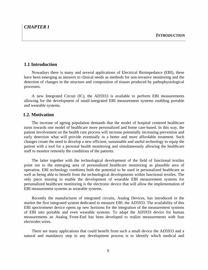
1.1 Introduction

Nowadays there is many and several applications of Electrical Bioimpedance (EBI), these

have been emerging as answers to clinical needs as methods for non-invasive monitoring and the

detection of changes in the structure and composition of tissues produced by pathophysiological

processes.

A new Integrated Circuit (IC), the AD5933 is available to perform EBI measurements

allowing for the development of small-integrated EBI measurement systems enabling portable

and wearable systems.

1.2. Motivation

The increase of ageing population demands that the model of hospital centered healthcare

turns towards one model of healthcare more personalized and home care-based. In this way, the

patient involvement on the health care process will increase potentially increasing prevention and

early detection what will provide eventually in a better and more affordable treatment. Such

changes create the need to develop a new efficient, sustainable and useful technology to equip the

patient with a tool for a personal health monitoring and simultaneously allowing the healthcare

staff to monitor remotely the conditions of the patients.

The latter together with the technological development of the field of functional textiles

point out to the emerging area of personalized healthcare monitoring as plausible area of

operation. EBI technology combines both the potential to be used in personalized healthcare as

well as being able to benefit from the technological developments within functional textiles. The

only piece missing to enable the development of wearable EBI measurement systems for

personalized healthcare monitoring is the electronic device that will allow the implementation of

EBI measurement systems as wearable systems.

Recently the manufacturer of integrated circuits, Analog Devices, has introduced in the

market the first integrated system dedicated to measure EBI: the AD5933. The availability of this

EBI spectrometer device opens up new horizons for the integration of the measurement systems

of EBI into portable and even wearable systems. To adapt the AD5933 device for human

measurements an Analog Front-End has been developed to realize measurements with four

electrodes wires.

There are many applications that could benefit from such a small device the AD5933 and a

natural and mandatory step in any development process is to identify which medical and

10

healthcare applications of EBI are potential candidates to benefit from the use AD5933-based

systems.

1.3. Goal

The main goal of this thesis is to identify the EBI applications suitable to be implemented

with an AD5933 enabled system.

1.4. Work done

As previously mentioned, this project is focused on the identification of applications of EBI

suitable to be implemented with the set AD5933 + 4E-AFE. In order to reach the mentioned goal,

the following work has been done:

Experimental EBI Measurements have been taken with the device SFB7 in a healthy

subject for the following EBI applications:

o Total Body Composition (TBC)

o Respiration Rate (RR)

o Lungs Composition (LC)

o Segmental Body Composition (SBC)

Arm-Arm (AA)

Leg-Leg (LL)

Trunk-Trunk (TT)

Experimentally based electrical 2R1C models equivalent to each EBI application have

been built.

The AD5933+4E-AFE has been customized by adjusting the values of internal

components to each of the applications.

For comparison purposes Impedance measurements on each of the built 2R1C model

have been performed with both the AD5933+4E-AFE device and the SFB7 Spectrometer.

All the obtained measurements, from both spectrometers, have been processed and a

performance comparison has been done based on the bias error obtained on the estimation

of the value of the original model parameters.

1.5. Structure of the Thesis Report

This thesis report is organized in 6 chapters and a final section for the references. Chapter 1

contains the introduction part of this thesis report. Chapter 2 provides a brief background EBI, the

measurement methods and the applications. Chapter 3 describes the instrumentation and the

methods used in this thesis while Chapter 4 shows the obtained results. Finally, Chapter 5

11

discusses the results and the work done and Chapter 6 ends the report with the conclusion and

proposal for future work.

1.6. Out of Scope

The following issues have not covered during this thesis work because they have been

considerate outside the scope of the project:

- To implement a new embedded system and software with the purpose to implement an

automatic customization of the AD5933 +4F-AFE.

- To test for the plausibility of EBI applications those require short time-continuous

measurements like impedance cardiography (ICG).

12

CHAPTER 2

BACKGROUND

2.1. Introduction to Electrical Bioimpedance

2.1.1. Historical Introduction

The first reported contact with the electrical properties of biological tissue was done by Luigi

Galvani [1], who on 1780 observed that while an assistant was touching the sciatic nerve of a frog

with a metal scalpel, the frog‟s muscle moved when he drew electric arcs on a nearby

electrostatic machine.

After several developments in electronic instrumentation like the Volta electrochemical

battery as the Continuous DC current source developed by Volta in 1800, the galvanometer from

1820, high AC voltage/current pulse generators from 1831 and the continuous AC current sources

from 1867, the detection of small bioelectrical currents became possible.

It was not until 1921 that Phillippson [4] made the first tissue impedance measurement as a

function of frequency, and found that the capacitance varied approximately as the inverse square

root of the frequency. After that, Fricke in 1924 [5] proposed an electrical equivalent model of

Bioimpedance for tissue and blood, here he assumed that cell are electrically represented by a

resistance Ri, intracellular fluid and capacitance C, cell membrane, in series and a resistance Re

representing the extracellular fluid in parallel. In 1928, 4 years before the publication of Fricke,

Kenneth S. Cole [6] found the expressions for the impedance at DC and infinite frequency and

paved the way for an analytical and mathematical treatment of tissue immittivity and permittivity.

Therefore, the first application of bioimpedance techniques for monitoring applications

appeared as early as 1940, impedance cardiography [7]. Since then, bioimpedance measurements

have been used in several medical applications; examples from a long list are lung function

monitoring [8], body composition [9] and skin cancer detection [10].

2.1.2. Electricals Properties of Biological Tissue

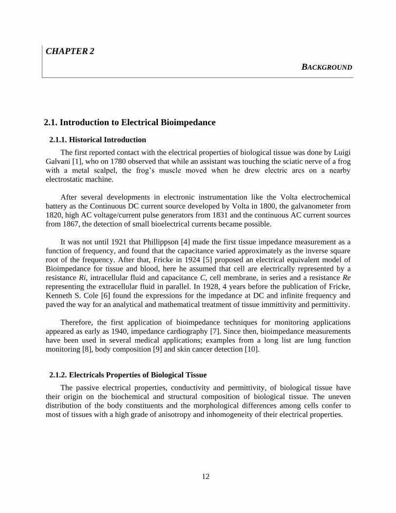
The passive electrical properties, conductivity and permittivity, of biological tissue have

their origin on the biochemical and structural composition of biological tissue. The uneven

distribution of the body constituents and the morphological differences among cells confer to

most of tissues with a high grade of anisotropy and inhomogeneity of their electrical properties.

13

Most often biological tissues are composed by group of cells, which are surrounded by a cell

membrane containing the intracellular fluid inside the cell membrane, that are suspended on

extracellular fluid. Both intracellular and extracellular fluids are rich in proteins and electrolytes,

see Table 2.1 Such composition provides them with ionic conductivity and are often modeled,

from an electrical point of view, as a conductance.

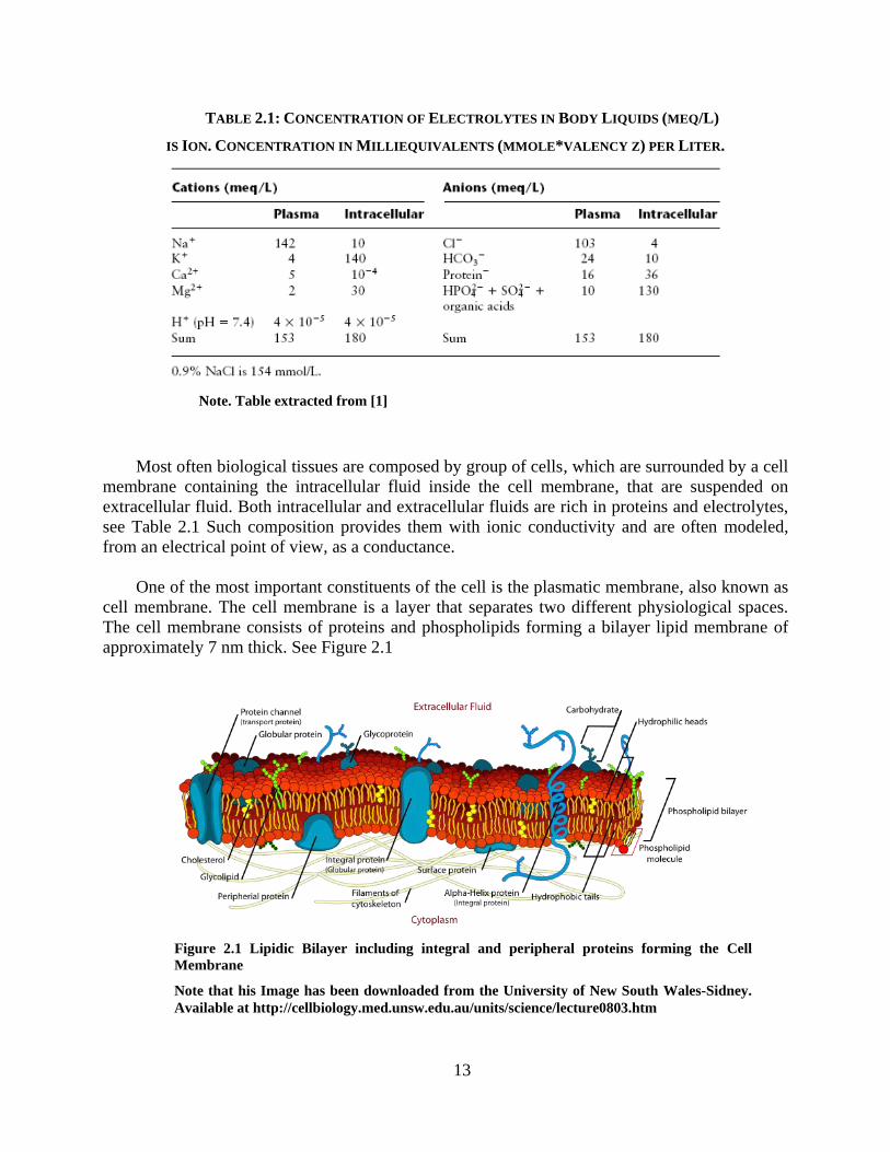
One of the most important constituents of the cell is the plasmatic membrane, also known as

cell membrane. The cell membrane is a layer that separates two different physiological spaces.

The cell membrane consists of proteins and phospholipids forming a bilayer lipid membrane of

approximately 7 nm thick. See Figure 2.1

TABLE 2.1: CONCENTRATION OF ELECTROLYTES IN BODY LIQUIDS (MEQ/L)

IS ION. CONCENTRATION IN MILLIEQUIVALENTS (MMOLE*VALENCY Z) PER LITER.

Note. Table extracted from [1]

Figure 2.1 Lipidic Bilayer including integral and peripheral proteins forming the Cell

Membrane

Note that his Image has been downloaded from the University of New South Wales-Sidney.

Available at http://cellbiology.med.unsw.edu.au/units/science/lecture0803.htm

14

Each monolayer has its hydrophobic surface oriented inward and its hydrophilic surface

outward towards either the intra- or extracellular fluids. The intrinsic electrical conductance of

this structure is very poor, of the order or 10-6

S/m and it is considered as a dielectric material. An

important property of a dielectric is its ability to support an electrostatic field and therefore

storage energy. The total structure formed by the intracellular fluid, plasma membrane and

extracellular fluid forms a conductor-dielectric-conductor alike structure behaving as a capacitor,

with an approximate capacitance of 1 µF/cm2.

2.1.3. The Dispersion Windows

The passive electric properties of biological tissue present certain dependency on the

frequency. Therefore the frequency spectrum of the electrical conductivity and permittivity is not

constant presenting four transition regions, which are known as dispersion windows, can be

observed. The classification of the dispersion windows is based on the electrical examination of

biomaterials as a function of frequency that is known as dielectric spectroscopy. H.P. Schwan

divided the relaxation mechanisms initially in 3 groups, [11] and later in 4 groups, providing the

four identified dispersion windows. Known as α, β, and γ-dispersions.; see Figure 2.2.

2.2. Measurements of Electrical Bioimpedance

2.2.1. The Cell Membrane

The electrical properties of the tissular constituents confer a frequency dependency to the

electrical bioimpedance and therefore any proper equivalent electrical models should represent

such dependency. H. Fricke in 1924 [5] proposed a simple electrical equivalent model made by

resistors and capacitors, see Figure 2.3.

In Figure 2.3 a) and b) the capacitor Cm represents the membrane, Rm represents the

resistance of the ionic channels (high value due to their low conductivity) and Re and Ri represent

the extra cellular and intracellular fluids respectively. Fricke‟s model is depicted in Figure 2.3 c)

Figure 2.2 Frequency dependence of the conductivity and permittivity of brain grey matter. Plots from [3]

15

and notice that the resistance of the membrane has been neglected due to its extremely large

value.

The impedance spectrum of a cell according to Fricke‟s model is given by the following

equation:

(2.1)

According to this simplified model, the electrical behavior at high and low frequencies can

be explained as follows:

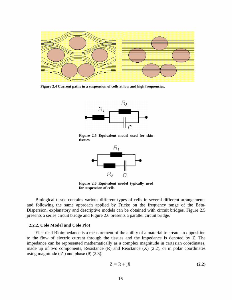
At low frequency, the membrane impedance is very high and only a small portion of the

current flows through the cells and most of the current flows through the extracellular

fluid as shown in the left side of Figure 2.4. Therefore the impedance is represented by

only Re.

At high frequency, the capacitive effect of the plasma membrane decreases and the

current flows through the intra and the extracellular fluid as shown in the right side of

Figure 2.4. Thus, the value of the equivalent impedance becomes the parallel between

resistances of the intra and the extracellular fluid, Ri||Re.

Figure 2.3 Equivalent circuit of a cell where Re is the extracellular fluid Resistance, Ri the intracellular fluid

Resistance, Rm the trans-membrane ionic channel Resistance and Cm represents the cell membrane

Capacitance.

16

Biological tissue contains various different types of cells in several different arrangements

and following the same approach applied by Fricke on the frequency range of the Beta-

Dispersion, explanatory and descriptive models can be obtained with circuit bridges. Figure 2.5

presents a series circuit bridge and Figure 2.6 presents a parallel circuit bridge.

2.2.2. Cole Model and Cole Plot

Electrical Bioimpedance is a measurement of the ability of a material to create an opposition

to the flow of electric current through the tissues and the impedance is denoted by Z. The

impedance can be represented mathematically as a complex magnitude in cartesian coordinates,

made up of two components, Resistance (R) and Reactance (X) (2.2), or in polar coordinates

using magnitude (|Z|) and phase (θ) (2.3).

(2.2)

Figure 2.4 Current paths in a suspension of cells at low and high frequencies.

Figure 2.5 Equivalent model used for skin

tissues

Figure 2.6 Equivalent model typically used

for suspension of cells

17

(2.3)

The electrical impedance of linear systems is ruled by Ohm‟s law, which relates voltage in

volts and current in Amperes through an impedance in Ohms, as denoted in (2.4).

(2.4)

Based in Ohm‟s law, a deflection method to measure electrical bioimpedance consist on

applying electrical current or voltage on the tissue and measure the response of the tissue to the

electrical stimulus. Like the input value over the impedance load is know and the complementary

value is measured, it is possible to obtain the value of the impedance load with Ohm‟s law. Most

often the electrical stimulus is applied into the tissue through electrodes and the electrical

response is also measured with electrodes. Therefore in order to do EBI measurements there are

several electrode configurations available and some of them they will be explained in the

following section.

2.2.3. Electrode configuration

There are several electrode configurations, but in this section only two will be explained:

The 2-Electrode and 4-Electrode configuration, which are the configuration relevant to this work.

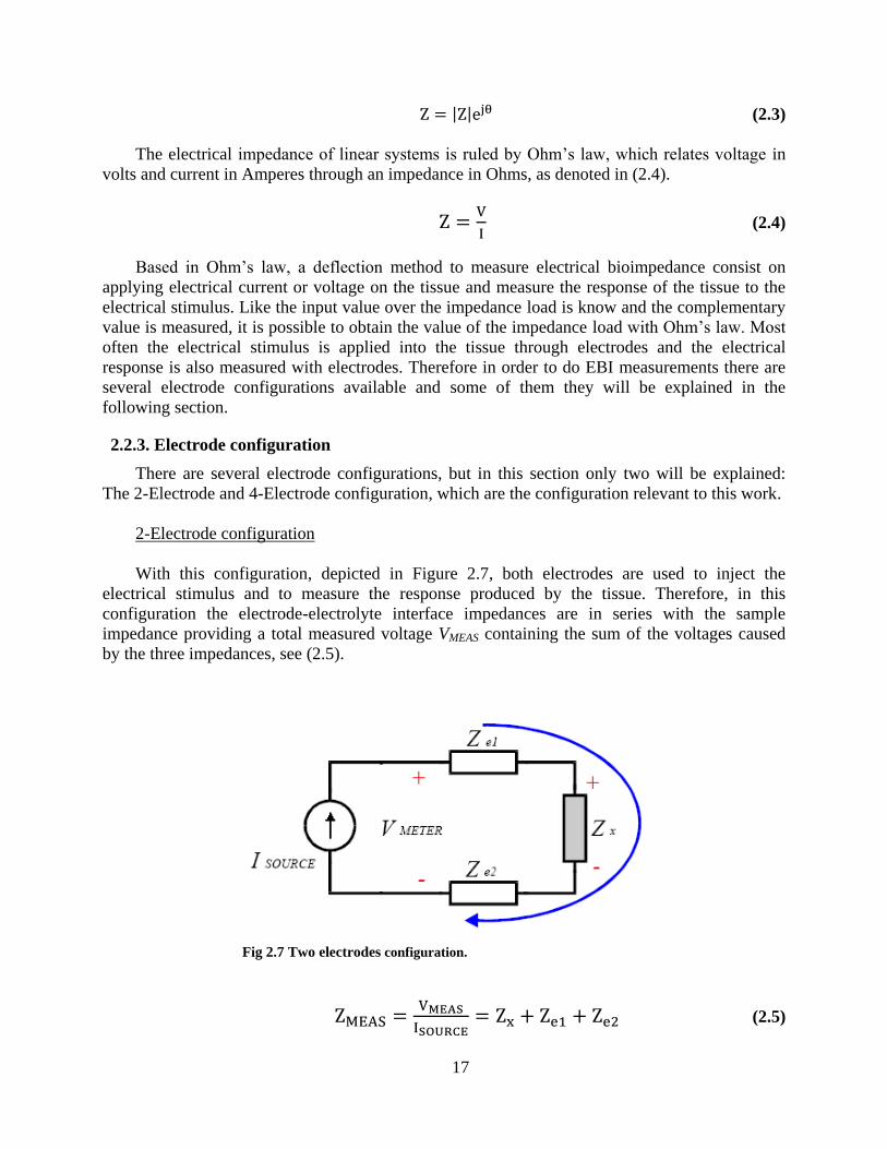
2-Electrode configuration

With this configuration, depicted in Figure 2.7, both electrodes are used to inject the

electrical stimulus and to measure the response produced by the tissue. Therefore, in this

configuration the electrode-electrolyte interface impedances are in series with the sample

impedance providing a total measured voltage VMEAS containing the sum of the voltages caused

by the three impedances, see (2.5).

(2.5)

Fig 2.7 Two electrodes configuration.

18

Therefore the impedance obtained by applying Ohm‟s law is the combination of the tissue

impedance together with the electrode impedance. Unfortunately, these impedances can be

difficult or almost impossible to separate and alternative measurement method must be used: The

4-Electrode configuration.

4-Electrode configuration

In this method the electrical stimulus is applied with a pair of electrodes and the resulting

response is measured with a different pair of electrodes, see Figure 2.8. Focusing on a current

driven system, the voltage on the current injecting electrodes is not contained in the voltage

response sensed by the system, therefore the influence of the electrodes impedance can be

reduced (2.6).

(2.6)

2.3. Applications of Bioimpedance

To analyze EBI data for each of the applications that have been studied in this work, several

approaches are available. In this section several methods used to obtain Body Composition

parameters as well as the applications of Respiration Rate and Lungs Composition will be

introduced.

2.3.1. Body Composition

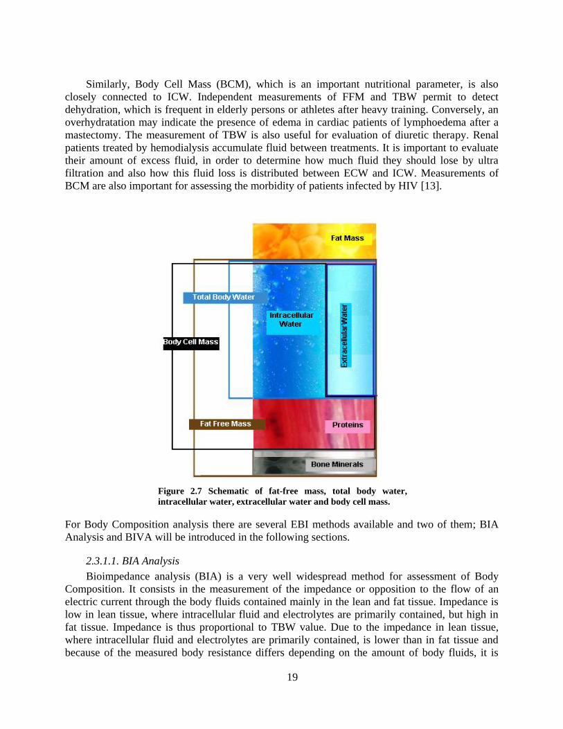
The measurement of body fluid volumes, see Figure 2.7, Extra Cellular Water (ECW), Intra

Cellular Water (ICW) and their sum, total body water (TBW) is important in many pathologies.

TBW is strongly related to Fat-Free-Mass (FFM) which contains, in healthy individuals, an

average of 73.2% of water [12].

Figure 2.8 Four electrodes configuration for a current driven system

19

Similarly, Body Cell Mass (BCM), which is an important nutritional parameter, is also

closely connected to ICW. Independent measurements of FFM and TBW permit to detect

dehydration, which is frequent in elderly persons or athletes after heavy training. Conversely, an

overhydratation may indicate the presence of edema in cardiac patients of lymphoedema after a

mastectomy. The measurement of TBW is also useful for evaluation of diuretic therapy. Renal

patients treated by hemodialysis accumulate fluid between treatments. It is important to evaluate

their amount of excess fluid, in order to determine how much fluid they should lose by ultra

filtration and also how this fluid loss is distributed between ECW and ICW. Measurements of

BCM are also important for assessing the morbidity of patients infected by HIV [13].

For Body Composition analysis there are several EBI methods available and two of them; BIA

Analysis and BIVA will be introduced in the following sections.

2.3.1.1. BIA Analysis

Bioimpedance analysis (BIA) is a very well widespread method for assessment of Body

Composition. It consists in the measurement of the impedance or opposition to the flow of an

electric current through the body fluids contained mainly in the lean and fat tissue. Impedance is

low in lean tissue, where intracellular fluid and electrolytes are primarily contained, but high in

fat tissue. Impedance is thus proportional to TBW value. Due to the impedance in lean tissue,

where intracellular fluid and electrolytes are primarily contained, is lower than in fat tissue and

because of the measured body resistance differs depending on the amount of body fluids, it is

Figure 2.7 Schematic of fat-free mass, total body water,

intracellular water, extracellular water and body cell mass.

20

possible to estimate the body composition. The basic model of this method is depicted in Figure

2.8 and it is based on the assumption that the body is a cylindrical-shape ionic conductor. In such

volume conductor, the impedance between faces of a cylinder of finite length L and a cross

sectional area A, when a uniform current density is applied parallel to its axis, is given by (2.7)

(2.7)

The measured impedance is a function of both the tissue complex resistivity ρ and also the

shape of the conductor. Although the body is not a uniform cylinder and its

conductivity/resistivity is not constant, a relationship between the volume of body water (V) and

the ratio length (L) to impedance can be established as in equations (2.8) and (2.9) [14].

(2.8)

(2.9)

It is easier to measure height than the conductive length, which is usually from wrist to

ankle. Therefore, the empirical relationship denoted as in the equation 2.10.

(2.10)

Due to the inherent inhomogeneity of the human body, and that (2.9) holds true for a

homogeneous cylinder, the coefficient K in (2.10) describes an equivalent cylinder, which must

be adjusted to match the real geometry. The value of the coefficient depends on various factors.

More information can be obtained reading [15].

Figure 2.8 Principles of BIA from physical characteristics to body composition. Cylinder model for the

relationship between impedance and geometry.

21

With the aim to obtain the body composition parameters the follow BIA methods are

currently used:

Single Frequency-BIA

Multi Frequency-BIA

Spectroscopy-BIA

Segmental-BIA

2.3.1.2. Single Frequency BIA

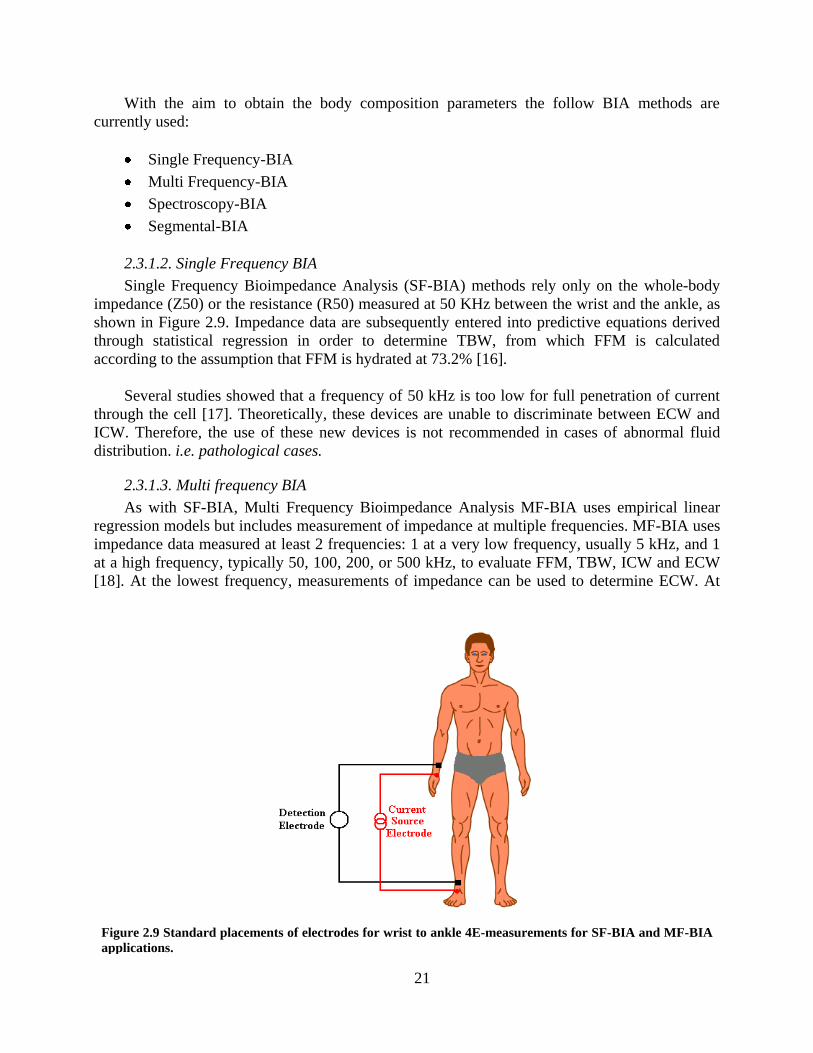
Single Frequency Bioimpedance Analysis (SF-BIA) methods rely only on the whole-body

impedance (Z50) or the resistance (R50) measured at 50 KHz between the wrist and the ankle, as

shown in Figure 2.9. Impedance data are subsequently entered into predictive equations derived

through statistical regression in order to determine TBW, from which FFM is calculated

according to the assumption that FFM is hydrated at 73.2% [16].

Several studies showed that a frequency of 50 kHz is too low for full penetration of current

through the cell [17]. Theoretically, these devices are unable to discriminate between ECW and

ICW. Therefore, the use of these new devices is not recommended in cases of abnormal fluid

distribution. i.e. pathological cases.

2.3.1.3. Multi frequency BIA

As with SF-BIA, Multi Frequency Bioimpedance Analysis MF-BIA uses empirical linear

regression models but includes measurement of impedance at multiple frequencies. MF-BIA uses

impedance data measured at least 2 frequencies: 1 at a very low frequency, usually 5 kHz, and 1

at a high frequency, typically 50, 100, 200, or 500 kHz, to evaluate FFM, TBW, ICW and ECW

[18]. At the lowest frequency, measurements of impedance can be used to determine ECW. At

Figure 2.9 Standard placements of electrodes for wrist to ankle 4E-measurements for SF-BIA and MF-BIA

applications.

22

higher frequencies, the current can pass through the cell membrane, and thus, the impedance

measurements can be used to determine TBW. The impedance data are applied to regression-

derived equations in order to predict TBW, ECW, and ICW. According to [19] MFBIA is more

accurate and less biased than SF-BIA for the prediction of ECW, whereas SF-BIA, compared to

MF-BIA, is more accurate and less biased for TBW in critically ill subjects. [20].

2.3.1.4. Spectroscopy BIA

Spectroscopy Bioimpedance Analysis operates on impedance data measured over a wide

spectrum of frequencies, usually from 5 to 1000 kHz. To analyze the BIS-derived impedance

data, the most practical approach for clinical applications is to perform biophysical modeling on

the impedance data; the modeling procedure involves fitting the spectral data to the Cole model

using nonlinear curve fitting [21] [13]. This procedure generates the Cole model parameters, as

well as R0, R , and exponent α. Cole model terms are then applied to equations derived from

the Hanai mixture theory [22], which is essentially based on the notion that the body is a

conducting medium of water, electrolytes, and lean tissue, in addition to non-conducting material

within it. ECW and ICW are thus calculated individually; TBW is calculated as the sum of ECW

and ICW.

Bioimpedance Spectroscopy Analysis provides a more direct, individualized measurement of

ECW and ICW than other bioimpedance approaches. This is due, in large part, to the fact that it

measures impedance over a broad spectrum of frequencies, rather than being limited to only 1 or

2 frequencies, like in the case of SF-BIA and MF-BIA, respectively. Of particular importance,

BIS differs from SF-BIA and MF-BIA in that it does not rely on statistically derived regression

equations to predict body water volumes. Furthermore, it relies far less on assumptions that may

be violated in disease states. For example, 2 assumptions underlying the SF-BIA method that may

not hold true in many clinical populations are that FFM is 73% hydrated and that ICW and ECW

are normally distributed.

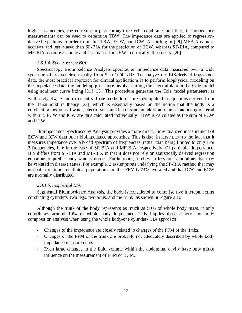
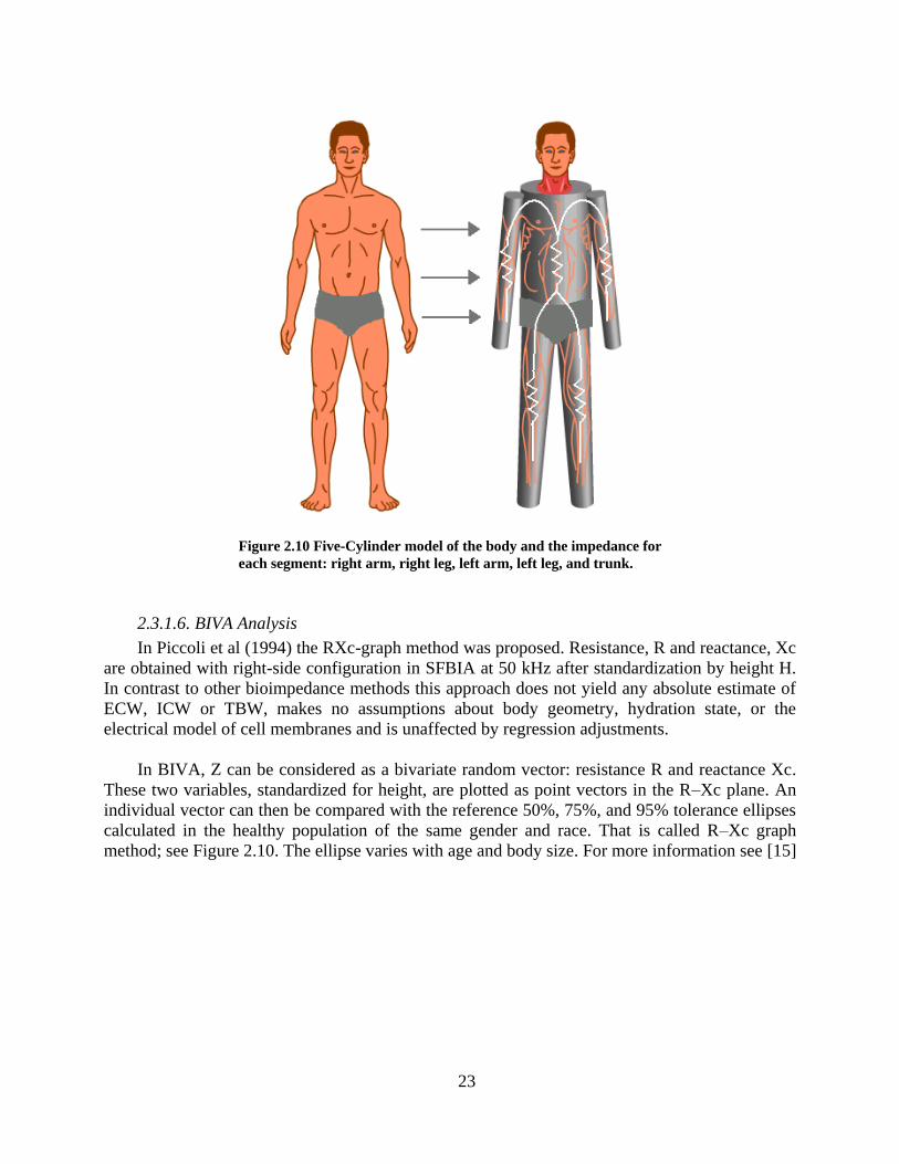
2.3.1.5. Segmental BIA

Segmental Bioimpedance Analysis, the body is considered to comprise five interconnecting

conducting cylinders, two legs, two arms, and the trunk, as shown in Figure 2.10.

Although the trunk of the body represents as much as 50% of whole body mass, it only

contributes around 10% to whole body impedance. This implies three aspects for body

composition analysis when using the whole body-one cylinder- BIA approach:

- Changes of the impedance are closely related to changes of the FFM of the limbs.

- Changes of the FFM of the trunk are probably not adequately described by whole body

impedance measurements

- Even large changes in the fluid volume within the abdominal cavity have only minor

influence on the measurement of FFM or BCM.

23

2.3.1.6. BIVA Analysis

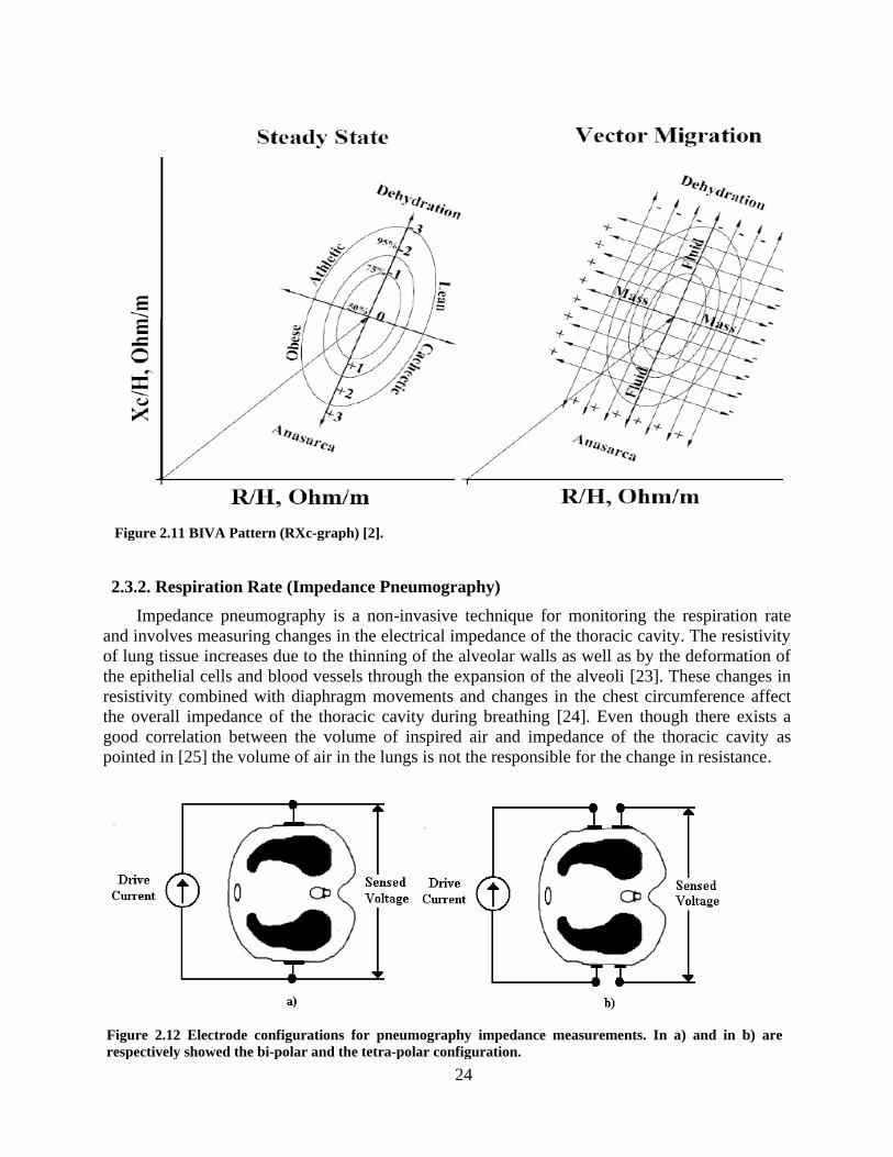
In Piccoli et al (1994) the RXc-graph method was proposed. Resistance, R and reactance, Xc

are obtained with right-side configuration in SFBIA at 50 kHz after standardization by height H.

In contrast to other bioimpedance methods this approach does not yield any absolute estimate of

ECW, ICW or TBW, makes no assumptions about body geometry, hydration state, or the

electrical model of cell membranes and is unaffected by regression adjustments.

In BIVA, Z can be considered as a bivariate random vector: resistance R and reactance Xc.

These two variables, standardized for height, are plotted as point vectors in the R–Xc plane. An

individual vector can then be compared with the reference 50%, 75%, and 95% tolerance ellipses

calculated in the healthy population of the same gender and race. That is called R–Xc graph

method; see Figure 2.10. The ellipse varies with age and body size. For more information see [15]

Figure 2.10 Five-Cylinder model of the body and the impedance for

each segment: right arm, right leg, left arm, left leg, and trunk.

24

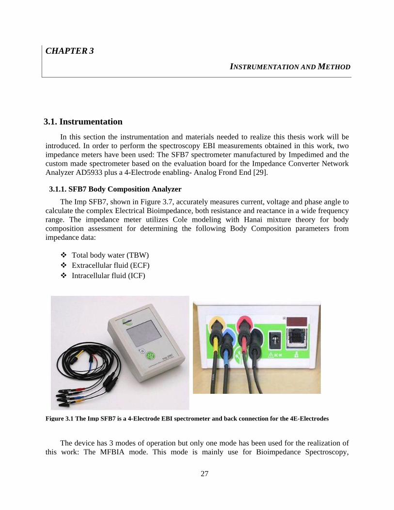
2.3.2. Respiration Rate (Impedance Pneumography)

Impedance pneumography is a non-invasive technique for monitoring the respiration rate

and involves measuring changes in the electrical impedance of the thoracic cavity. The resistivity

of lung tissue increases due to the thinning of the alveolar walls as well as by the deformation of

the epithelial cells and blood vessels through the expansion of the alveoli [23]. These changes in

resistivity combined with diaphragm movements and changes in the chest circumference affect

the overall impedance of the thoracic cavity during breathing [24]. Even though there exists a

good correlation between the volume of inspired air and impedance of the thoracic cavity as

pointed in [25] the volume of air in the lungs is not the responsible for the change in resistance.

Figure 2.11 BIVA Pattern (RXc-graph) [2].

Figure 2.12 Electrode configurations for pneumography impedance measurements. In a) and in b) are

respectively showed the bi-polar and the tetra-polar configuration.

25

These impedance changes are measured by injecting a low-amplitude, single high-frequency,

constant current using a pair of „drive‟ electrodes and recording the resultant voltage changes

either from the same pair of electrodes as in a 2-Electrode (bi-polar) configuration in the Figure

2.12.a or from a different pair of „receive‟ electrodes placed at an appropriate location as in a 4-

Electrode (tetra-polar) configuration in the Figure 2.12.b [26].

Impedance pneumography is well tolerated by patients because it does not involve placing

any device within the airway that may cause discomfort to the patient. Therefore, it is the most

widely used technique for the purpose of long-term monitoring and home monitoring.

2.3.3. Lungs Composition (Impedance Plethysmography)

The impedance plethysmography is a non-invasive technique used to detect the changes of

the thoracic impedance. It is known that changes of the thoracic impedance correlate with

changes of the clinical syndromes of a lung edema due to the accumulation of fluid in the lungs

[27] [28], see Figure 2.13. Furthermore, the thoracic impedance decreases considerably before the

first clinical syndromes appear. So lung edema can be well detected using impedance

plethysmography during their appearance and disappearance.

The electrode placement for measurements of lung edema is under investigation, but there

are two methods commonly used. The first method is the tetra polar configuration, as the Figure

2.14.a shows and the other method uses 6 electrodes in the specific placement as shows the

Figure 2.14.b.

Figure 2.13 The figure illustrates in the left hand normal lungs and in the right hand lungs with Pulmonary

Edema. The light blue color on the right side drawing represents water.

26

Figure 2.14 Thoracic bioimpedance measured in the tetra polar configuration in a) and the with six

electrodes configuration in b).

27

CHAPTER 3

INSTRUMENTATION AND METHOD

3.1. Instrumentation

In this section the instrumentation and materials needed to realize this thesis work will be

introduced. In order to perform the spectroscopy EBI measurements obtained in this work, two

impedance meters have been used: The SFB7 spectrometer manufactured by Impedimed and the

custom made spectrometer based on the evaluation board for the Impedance Converter Network

Analyzer AD5933 plus a 4-Electrode enabling- Analog Frond End [29].

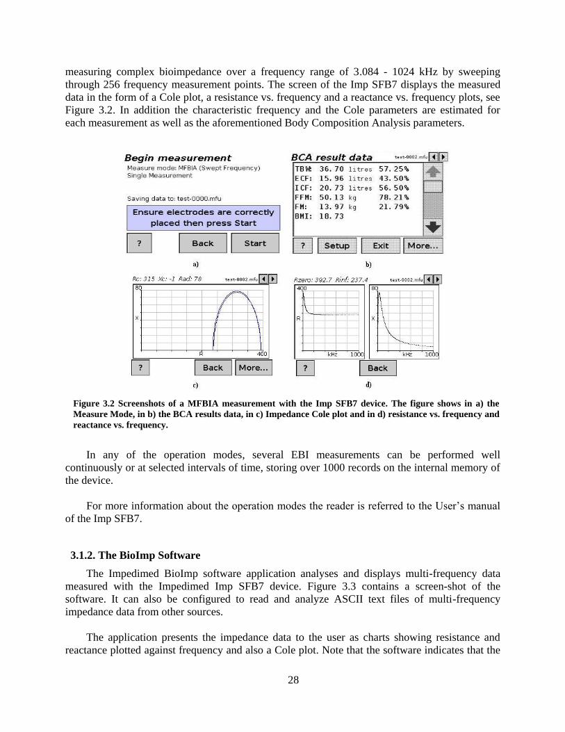
3.1.1. SFB7 Body Composition Analyzer

The Imp SFB7, shown in Figure 3.7, accurately measures current, voltage and phase angle to

calculate the complex Electrical Bioimpedance, both resistance and reactance in a wide frequency

range. The impedance meter utilizes Cole modeling with Hanai mixture theory for body

composition assessment for determining the following Body Composition parameters from

impedance data:

Total body water (TBW)

Extracellular fluid (ECF)

Intracellular fluid (ICF)

The device has 3 modes of operation but only one mode has been used for the realization of

this work: The MFBIA mode. This mode is mainly use for Bioimpedance Spectroscopy,

Figure 3.1 The Imp SFB7 is a 4-Electrode EBI spectrometer and back connection for the 4E-Electrodes

28

measuring complex bioimpedance over a frequency range of 3.084 - 1024 kHz by sweeping

through 256 frequency measurement points. The screen of the Imp SFB7 displays the measured

data in the form of a Cole plot, a resistance vs. frequency and a reactance vs. frequency plots, see

Figure 3.2. In addition the characteristic frequency and the Cole parameters are estimated for

each measurement as well as the aforementioned Body Composition Analysis parameters.

In any of the operation modes, several EBI measurements can be performed well

continuously or at selected intervals of time, storing over 1000 records on the internal memory of

the device.

For more information about the operation modes the reader is referred to the User‟s manual

of the Imp SFB7.

3.1.2. The BioImp Software

The Impedimed BioImp software application analyses and displays multi-frequency data

measured with the Impedimed Imp SFB7 device. Figure 3.3 contains a screen-shot of the

software. It can also be configured to read and analyze ASCII text files of multi-frequency

impedance data from other sources.

The application presents the impedance data to the user as charts showing resistance and

reactance plotted against frequency and also a Cole plot. Note that the software indicates that the

Figure 3.2 Screenshots of a MFBIA measurement with the Imp SFB7 device. The figure shows in a) the

Measure Mode, in b) the BCA results data, in c) Impedance Cole plot and in d) resistance vs. frequency and

reactance vs. frequency.

29

impedance plot is a Cole-Cole Plot but that is wrong, since the plot is in the impedance plot and

the Cole-Cole plot do not represents impedance data. The data analysis fits a Cole model curve to

the measured data, and derives body composition estimates from the Cole model. There are

adjustable input parameters for the fitting algorithm. The source data and analysis results can be

viewed in text form and in graphical form.

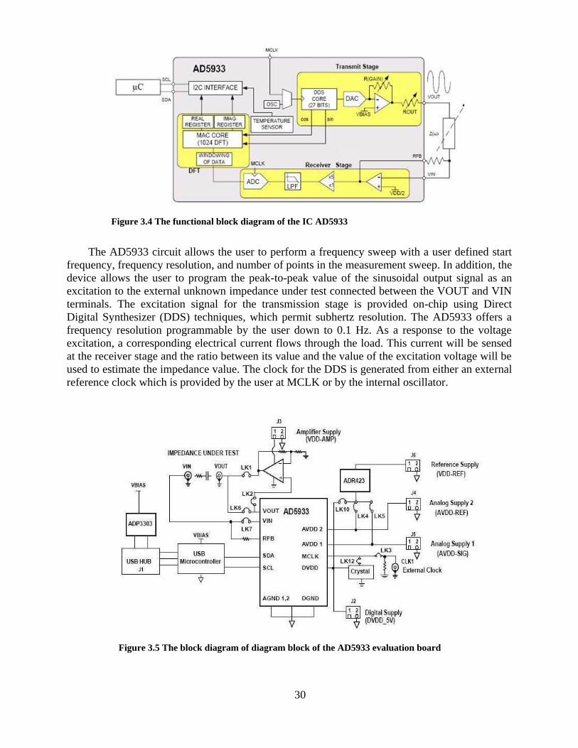
3.1.3. Evaluation Board for the Impedance Converter Network Analyzer AD5933

The main component of the evaluation board in Figure 3.6 is the IC manufactured by Analog

Devices: the AD5933, see functional block on Figure 3.4. The AD5933 is a 12-bit precision

impedance converter which combines an onboard frequency generator with a 1 MSPS Analog-to-

Digital Converter (ADC) and a Digital Signal Processor (DSP) engine which performs the

impedance estimation. The AD5933 operates from a 2.7 V to 5.5 V power supply. The evaluation

Board has the option to power up the entire circuitry from the USB port of the computer and it

has an accurately trimmed 16 MHz crystal to act as a system clock to the AD5933 as well, if it is

required.

The AD5933 includes a serial I2C port as communication interface that allows the adjusting

of several operational parameters as well as the transmission with an external Host of the

impedance data results. In order to make the interface between the I2C signals from the AD5933

with USB the board has a USB microcontroller that produces de I2C-USB conversion, see Figure

3.5.

Figure 3.3 The Impedimed BioImp applications displaying whole body bioimpedance data

from the Impedimed Imp SFB7 device.

30

The AD5933 circuit allows the user to perform a frequency sweep with a user defined start

frequency, frequency resolution, and number of points in the measurement sweep. In addition, the

device allows the user to program the peak-to-peak value of the sinusoidal output signal as an

excitation to the external unknown impedance under test connected between the VOUT and VIN

terminals. The excitation signal for the transmission stage is provided on-chip using Direct

Digital Synthesizer (DDS) techniques, which permit subhertz resolution. The AD5933 offers a

frequency resolution programmable by the user down to 0.1 Hz. As a response to the voltage

excitation, a corresponding electrical current flows through the load. This current will be sensed

at the receiver stage and the ratio between its value and the value of the excitation voltage will be

used to estimate the impedance value. The clock for the DDS is generated from either an external

reference clock which is provided by the user at MCLK or by the internal oscillator.

Figure 3.5 The block diagram of diagram block of the AD5933 evaluation board

Figure 3.4 The functional block diagram of the IC AD5933

31

For detailed information about the evaluation board for AD5933, please read the datasheets

of the AD5933 and the AD5933 evaluation board.

3.1.4. Four Electrodes Analog Front End

Since the AD5933 is a 2-Electrode measurements system and its electrical stimulation does

not comply with the safety regulations, the evaluation board is connected to an Analog Front-End

(AFE) circuit [29]. The functionality of this AFE is twofold:

- To ensure that the safety conditions regarding current injection for performing EBI

measurements in human patients are fulfilled. Basically this means that the electrical

signals are below any safety threshold and no DC current is introduced in the body.

- To adapt the AD5933 operation from a 2-Electrode measurement system to a 4-Electrode

measurement system. This way the polarization impedance of the electrodes is removed

from the EBI measurement and the system can be used in applications of spectral

characterization. The AFE is connected to the evaluation board through two cables and to

the patient through 4 electrodes.

In short, we could consider the AFE, see Figure 3.7, as a combination of two Voltage-to-

Current converters (V2CC), one in the direction from the AD5933 and another from the TUS to

the AD5933.

Figure 3.6 The evaluation board manufactured by Analog Devices.

32

Since the AD5933 applies voltage and expects a current at its input RFB, the AFE

interfacing with the AD5933 has a voltage input and a current output. Source output expressly

generates a current resulting from the ratio from Vout and the impedance of the Tissue Under

Study (TUS), which is the exactly the current expected by the AD5933 at the input RFB as

indicated in Figure 3.7. At the TUS side, the AFE has a current source as output, exciting the

TUS with 350 μA-rms, while the input is a differential voltage measurement channel.

In essence the AFE operation can be describe as follows: after the removal of the DC bias

component from the voltage output of the AD5933 with a low pass filter at the input of the first

V2CC, the AC voltage from Vout drives the Voltage Controlled Current Source (VCCS)

injecting an AC current Iout in the TUS directly proportional to Vout.

The second V2CC senses at its differential input the voltage drop caused at the TUS by the

AC current generated by the first V2CC flowing through the TUS. Finally an AC current

proportional to the voltage drop in the TUS is generated at the output of the second V2CC with

an added DC component equivalent to the DCbias removed originally from the Vout. The total

gain introduced by the cascade combination of both V2CC in the AFE is selectable by the

choosing of several resistors.

3.2. Method

In order to evaluate the performance of the Impedance Spectrometer On-chip AD5933 +4-

Electrode Analog Frond End (4E-AFE), Impedance spectroscopy measurements for several EBI

applications have been taken. Experimental measurements on electrical equivalent models have

been taken with the AD5933+4E-AFE system and the EBI spectrometer Impedimed SFB7. The

obtained impedance spectral data have been used to estimate the values of the equivalent circuit

under measurement and the estimated values have been mutually compared in terms of estimation

accuracy.

Figure 3.7 Functional block diagram of the Analog Front-End.

33

The measurements have been taken on 2R1C equivalent models [30], each of them

representing an specific EBI application. The electrical equivalence has been established both in

terms of frequency as well as Ohmic load dynamic range. The values of the passive electrical

components models were obtained experimentally from experimental EBI measurements. Since

the value of the working load depends on the EBI applications, the functioning of the

AD5933+4E-AFE was adjusted specifically to the impedance values range of each model. Figure

3.8 shows the work flow that has been applied in this work.

3.2.1. Application Equivalent Modeling

The equivalent circuit topology chosen to model the EBI applications has been the 2R1C

[30]. To obtain the values of the passive components for each specific equivalent model, the

following steps have taken:

1. Experimental Measurements. In this step EBI measurements have been taken in a

healthy subject for the following EBI applications:

- Total Body Water contents

- Lungs Composition

- Respiration Rate

- Segmental measurements for Body Composition:

Arm-Arm, Leg-Leg, Trunk-Trunk.

The specific morphological data of the subject is shown in Table 3.1.

The 4-Electrode EBI measurements were taken with the SFB7 spectrometer within

the frequency range 3 kHz to 1 MHz.

Figure 3.9 Modeling process overview

Experimental Measurements with SFB7

•Lungs

•RR

•TBC

•SBC

BIOIMP Circuit Modelling

•Averaging of 100 spectroscopy measurements for each application.

TABLE 3.1

Sex Age (years) Length(cm) Weight(Kg)

Male 24 173 79

34

2. BioImp 2R1C-paralell bridge Circuit Modeling. The obtained spectral impedance

data from each of the EBI application specific measurements were processed with

the BioImp software to obtain the values for the passive components of the

equivalent circuit model.

The obtained values and parameters obtained from each EBI applications are the

following:

- 2R1C model components:

o Intracellular Resistance (Ri)

o Extracellular Resistance (Re)

o Membrane Capacitor (Cm)

- Resistance at 0 Hz ( )

- Resistance at Hz( )

- Characteristic Frequency (Fc)

The final value for each of the parameters was obtained from the averaging of 100

spectroscopy measurements using the batch processing tool available at BioImp.

3.2.2 EBI Application Equivalent Load

Once typical values for the components of the 2R1C have been calculated by averaging the

experimentally performed EBI measurements, a typical dynamic range for the resistance was

obtained. The maximum value of the model is set by Re and the minimum is set by the parallel

connection of Re//Ri.

Since the circuit parameters have been obtained from a single subject and both Re and Ri

have an strong dependency on the size and the form of the tissue under study i.e. the whole body.

The values of the resistors of the 2R1C bridge have been adjusted considering for the variance in

morphological parameters of the population i.e. size, complexion, high etc. The applied process is

explained as follows in the next diagram, see Figure 3.10.

1. Increasing the Load Dynamic Range. The range of values of the load was

increased not directly over the 2R1C model but on the Cole parameters. Since the

EBI spectrometer measures bioimpedance down to 0 Ohms, the upper limit of the

range was adjusted modifying the value of R0. The new R0‟ value was obtained by

Figure 3.10 EBI Application Equivalent Load and Customization Process Overview

Increasing Load Dynamic Range

•RE=R0'=R0(1+α)

AD5933+4E-AFE application customization

•RG1, R4 and RRFB

35

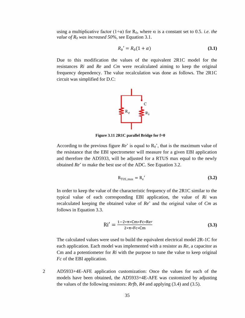
using a multiplicative factor (1+α) for R0, where is a constant set to 0.5. i.e. the

value of R0 was increased 50%, see Equation 3.1.

(3.1)

Due to this modification the values of the equivalent 2R1C model for the

resistances Ri and Re and Cm were recalculated aiming to keep the original

frequency dependency. The value recalculation was done as follows. The 2R1C

circuit was simplified for D.C:

According to the previous figure Re‟ is equal to R0‟, that is the maximum value of

the resistance that the EBI spectrometer will measure for a given EBI application

and therefore the AD5933, will be adjusted for a RTUS max equal to the newly

obtained Re‟ to make the best use of the ADC. See Equation 3.2.

(3.2)

In order to keep the value of the characteristic frequency of the 2R1C similar to the

typical value of each corresponding EBI application, the value of Ri was

recalculated keeping the obtained value of Re‟ and the original value of Cm as

follows in Equation 3.3.

(3.3)

The calculated values were used to build the equivalent electrical model 2R-1C for

each application. Each model was implemented with a resistor as Re, a capacitor as

Cm and a potentiometer for Ri with the purpose to tune the value to keep original

Fc of the EBI application.

2 AD5933+4E-AFE application customization: Once the values for each of the

models have been obtained, the AD5933+4E-AFE was customized by adjusting

the values of the following resistors: Rrfb, R4 and applying (3.4) and (3.5).

Figure 3.11 2R1C parallel Bridge for f=0

36

From the AC Analysis:

(3.4)

From the DC Analysis:

(3.5)

In order to make the most of the dynamic range of the ADC of the sensing stage of

the AD5933, a DC bias voltage was introduced at the input with the value. Solving

(3.6) for it was found that the values for Rrfb and R4 and must be equal.

(3.6)

(3.7)

(3.8)

(3.9)

By means of the AC analysis, an amplitude voltage at the input of the sensing stage

of 1.5 Volts was applied and the resistance RG1, the gain resistance of INA111 on

the 4E-AFE, was calculated with the Equation 3.10:

(3.10)

From the analysis, it was obtained that several parameters have common values for

all the EBI applications. The Table 3.2 lists the parameters with the corresponding

values common for the EBI applications:

TABLE 3.2

Rcc1 Resistor of the voltage-current converter amplifier 7.5KΩ

R4 Resistor current-voltage 10 KΩ

Rrfb Feedback resistor 10 KΩ

Vi Vac injection 1.98V

Vdd Vdc supply 3V

37

This way RG1 is the only parameter left that must be adjusted specifically to each

application. Table 3.3 lists each of the obtained values for RG1 for each EBI

application.

3.2.3 EBI Application Equivalent Spectroscopy Measurements

Hence, with the optimization of the system AD5933+4E-AFE already done, the impedance

measurements for each model were made with both devices: the SFB7 and the AD5933+4E-AFE.

3.2.3.1. SFB7 measurements.

100 spectroscopy measurements have been taken in the frequency range from

3kHz to 1MHz for each of the equivalent circuits. Each obtained spectrum was

saved in a text file, which contains the measurement frequency and both the

measured resistance and reactance. The SFB7 distributes the measurement

frequencies, exponentially distributing 256 measurement points between 3 kHz to

1 MHz. See Figure 3.12. This frequency distribution dedicates more measurement

points to lower frequencies than for higher frequencies.

TABLE 3.3

APPLICATION RG1(Ω)

TBC 6619

Arm-Arm 2851

Leg-Leg 3858

Trunk-Trunk 801

LC 654

RR 481

38

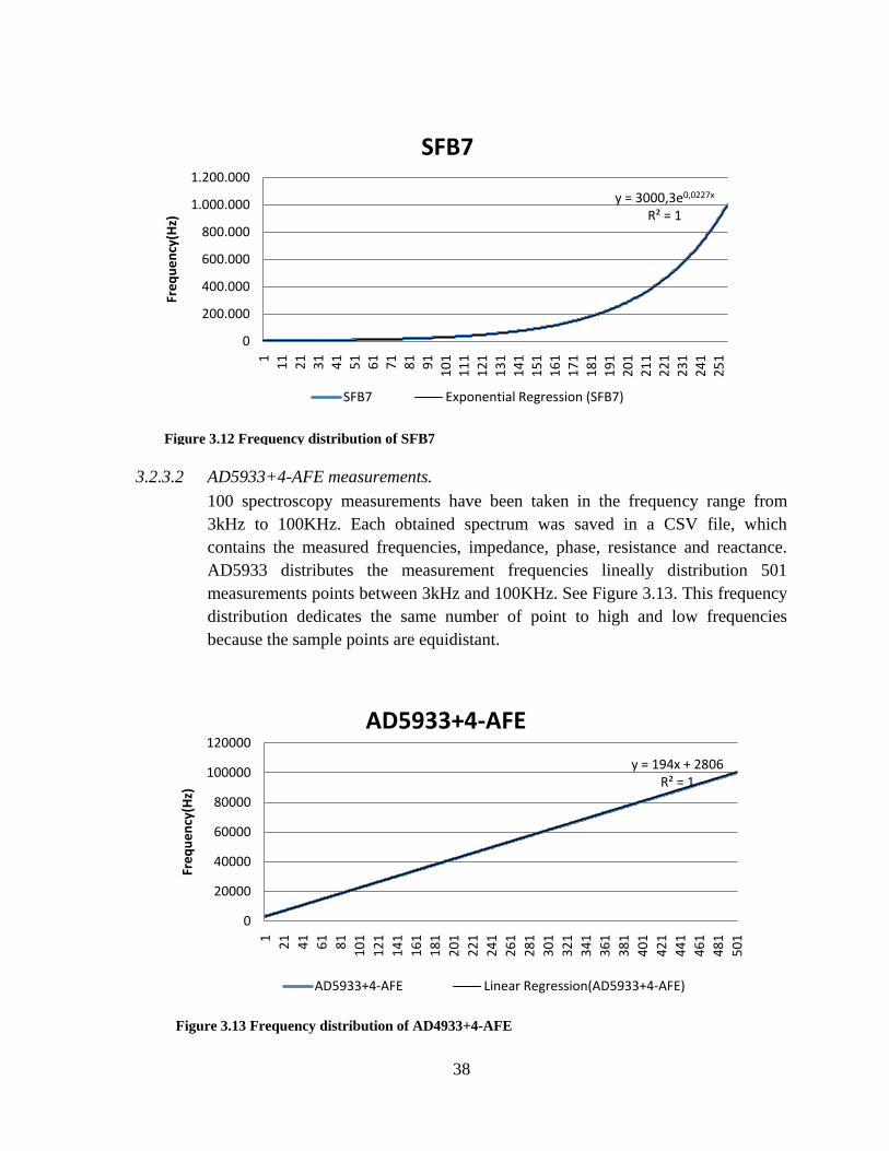
3.2.3.2 AD5933+4-AFE measurements.

100 spectroscopy measurements have been taken in the frequency range from

3kHz to 100KHz. Each obtained spectrum was saved in a CSV file, which

contains the measured frequencies, impedance, phase, resistance and reactance.

AD5933 distributes the measurement frequencies lineally distribution 501

measurements points between 3kHz and 100KHz. See Figure 3.13. This frequency

distribution dedicates the same number of point to high and low frequencies

because the sample points are equidistant.

Figure 3.12 Frequency distribution of SFB7

y = 3000,3e0,0227x

R² = 1

0

200.000

400.000

600.000

800.000

1.000.000

1.200.000

11

12

13

14

15

16

17

18

19

11

01

11

11

21

13

11

41

15

11

61

17

11

81

19

12

01

21

12

21

23

12

41

25

1

Fre

qu

en

cy(H

z)

SFB7

SFB7 Exponential Regression (SFB7)

Figure 3.13 Frequency distribution of AD4933+4-AFE

y = 194x + 2806R² = 1

0

20000

40000

60000

80000

100000

120000

1

21

41

61

81

10

1

12

1

14

1

16

1

18

1

20

1

22

1

24

1

26

1

28

1

30

1

32

1

34

1

36

1

38

1

40

1

42

1

44

1

46

1

48

1

50

1

Fre

qu

en

cy(H

z)

AD5933+4-AFE

AD5933+4-AFE Linear Regression(AD5933+4-AFE)

39

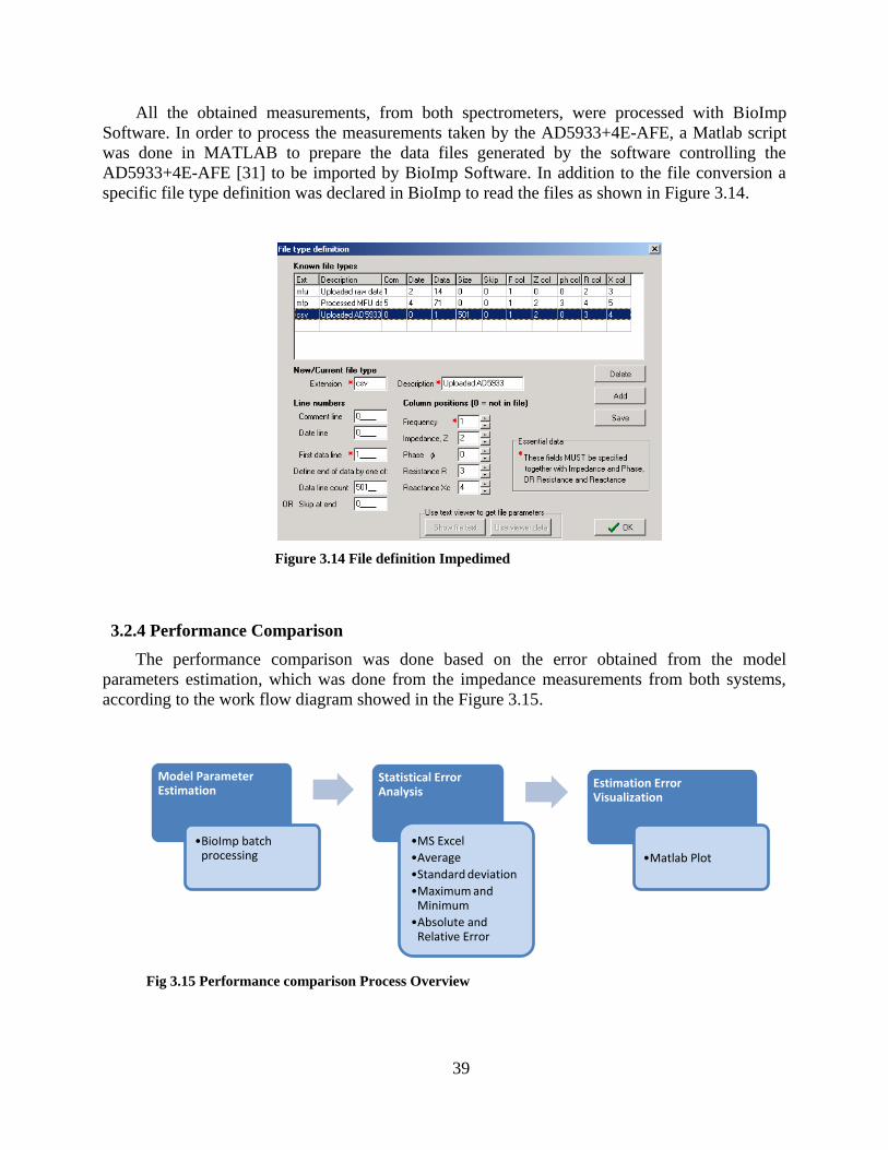
All the obtained measurements, from both spectrometers, were processed with BioImp

Software. In order to process the measurements taken by the AD5933+4E-AFE, a Matlab script

was done in MATLAB to prepare the data files generated by the software controlling the

AD5933+4E-AFE [31] to be imported by BioImp Software. In addition to the file conversion a

specific file type definition was declared in BioImp to read the files as shown in Figure 3.14.

3.2.4 Performance Comparison

The performance comparison was done based on the error obtained from the model

parameters estimation, which was done from the impedance measurements from both systems,

according to the work flow diagram showed in the Figure 3.15.

Figure 3.14 File definition Impedimed

Fig 3.15 Performance comparison Process Overview

Model Parameter Estimation

•BioImp batch processing

Statistical Error Analysis

•MS Excel

•Average

•Standard deviation

•Maximum and Minimum

•Absolute and Relative Error

Estimation Error Visualization

•Matlab Plot

40

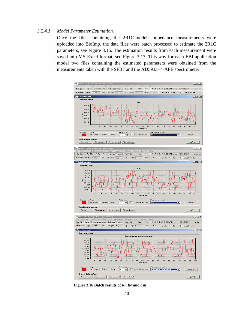
3.2.4.1 Model Parameter Estimation.

Once the files containing the 2R1C-models impedance measurements were

uploaded into BioImp, the data files were batch processed to estimate the 2R1C

parameters, see Figure 3.16. The estimation results from each measurement were

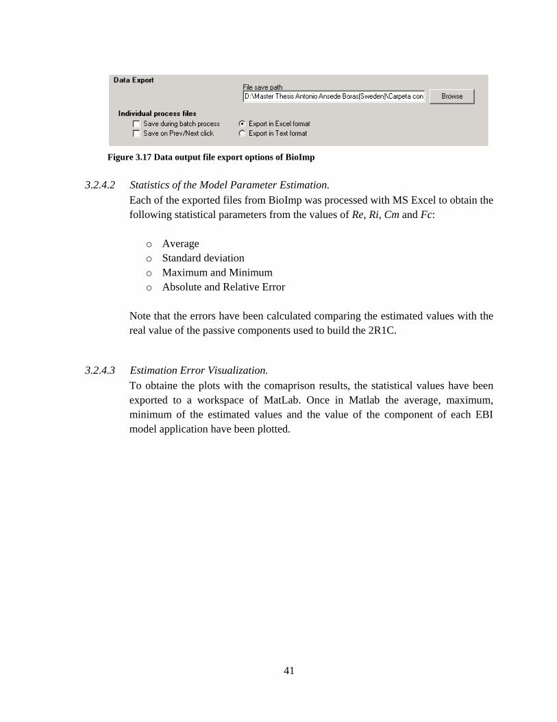
saved into MS Excel format, see Figure 3.17. This way for each EBI application

model two files containing the estimated parameters were obtained from the

measurements taken with the SFB7 and the AD5933+4-AFE spectrometer.

Figure 3.16 Batch results of Ri, Re and Cm

41

3.2.4.2 Statistics of the Model Parameter Estimation.

Each of the exported files from BioImp was processed with MS Excel to obtain the

following statistical parameters from the values of Re, Ri, Cm and Fc:

o Average

o Standard deviation

o Maximum and Minimum

o Absolute and Relative Error

Note that the errors have been calculated comparing the estimated values with the

real value of the passive components used to build the 2R1C.

3.2.4.3 Estimation Error Visualization.

To obtaine the plots with the comaprison results, the statistical values have been

exported to a workspace of MatLab. Once in Matlab the average, maximum,

minimum of the estimated values and the value of the component of each EBI

model application have been plotted.

Figure 3.17 Data output file export options of BioImp

42

CHAPTER 4

RESULTS

4.1 Overview

This chapter presents the results obtained from the measurements and the data analysis

performed as described in the previous chapter. Firstly, the EBI spectroscopy measurements for

each EBI application obtained with the SFB7 spectrometer will be shown by means of resistance

and reactance spectra. Secondly, the values of the equivalent 2R1C models estimated from the

initial obtained EBI spectroscopy measurements and the values of the implemented model will be

listed in terms of Re, Ri and Cm. Thirdly, the Impedance spectroscopy measurements taken from

the implemented 2R1C-equivalent models with, both the SFB7 and AD5933+4-AFE, will be

displayed represented as in the first point and finally, the comparison of both bioimpedance

spectroscopy (BIS) devices will be shown with different statistical graphs.

4.2 SFB7 Measurements

In order to obtain an electrical circuit equivalent to the EBI measurement scenarios under

study in this thesis work, experimental EBI Spectroscopy measurements have been taken and

they are shown in the following graphs. The spectrum of the resistance and the reactance for each

EBI scenario are plotted between in the frequency range 3 kHz to 1 MHz.

4.2.1 Total Body Composition (TBC):

In Figure 4.1 a) it is possible to observe that the maximum and minimum values of the resistance

are approximately 600 Ω and 418 Ω respectively providing us with a dynamic range of

approximately 182 Ω.

Figure 4.1 The spectra of the resistance and reactance are plotted respectively in a) and b). In b) it is

possible to observe that there is only one dominant dispersion with a Fc value approximately of 28 kHz

43

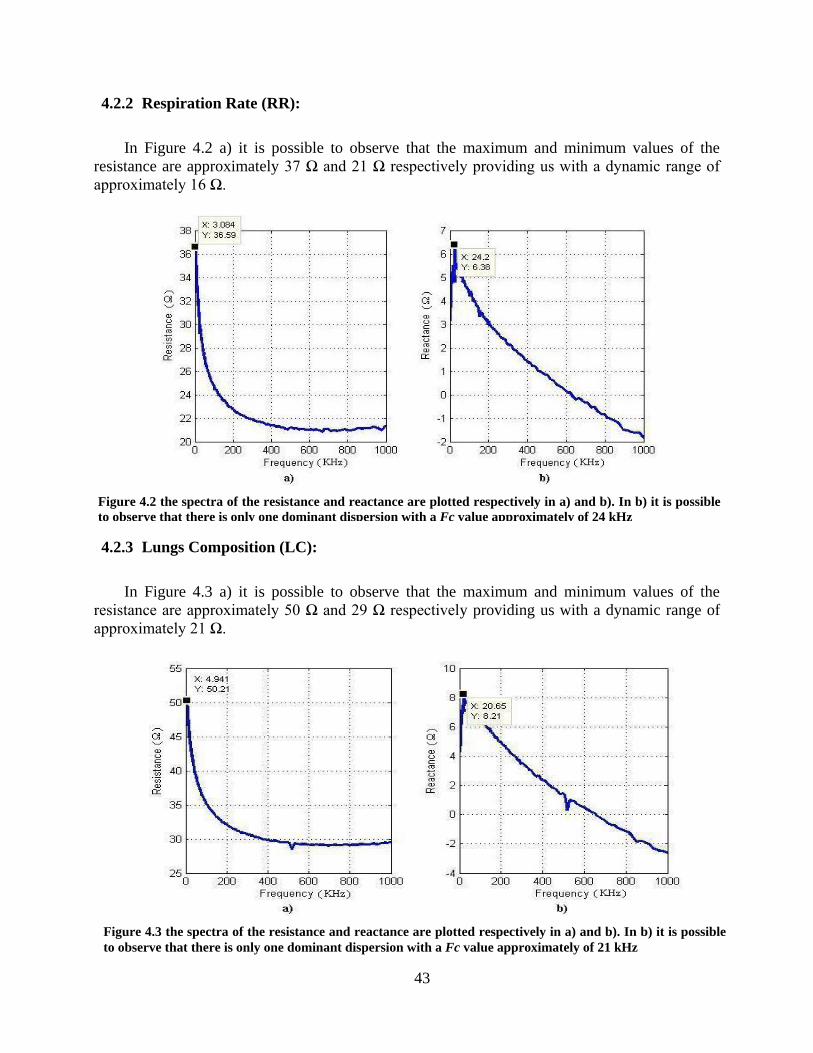
4.2.2 Respiration Rate (RR):

In Figure 4.2 a) it is possible to observe that the maximum and minimum values of the

resistance are approximately 37 Ω and 21 Ω respectively providing us with a dynamic range of


4.2.3 Lungs Composition (LC):




Figure 4.2 the spectra of the resistance and reactance are plotted respectively in a) and b). In b) it is possible

to observe that there is only one dominant dispersion with a Fc value approximately of 24 kHz



44

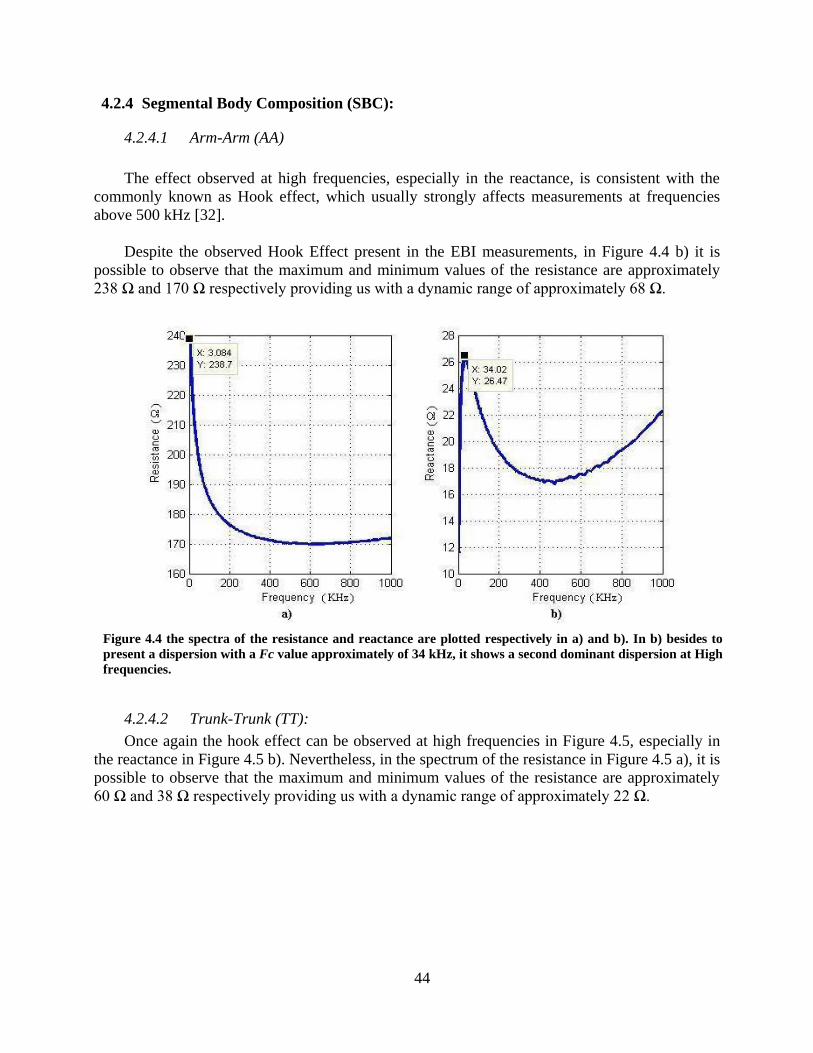
4.2.4 Segmental Body Composition (SBC):

4.2.4.1 Arm-Arm (AA)

The effect observed at high frequencies, especially in the reactance, is consistent with the

commonly known as Hook effect, which usually strongly affects measurements at frequencies

above 500 kHz [32].

Despite the observed Hook Effect present in the EBI measurements, in Figure 4.4 b) it is

possible to observe that the maximum and minimum values of the resistance are approximately

238 Ω and 170 Ω respectively providing us with a dynamic range of approximately 68 Ω.

4.2.4.2 Trunk-Trunk (TT):

Once again the hook effect can be observed at high frequencies in Figure 4.5, especially in

the reactance in Figure 4.5 b). Nevertheless, in the spectrum of the resistance in Figure 4.5 a), it is

possible to observe that the maximum and minimum values of the resistance are approximately

60 Ω and 38 Ω respectively providing us with a dynamic range of approximately 22 Ω.

Figure 4.4 the spectra of the resistance and reactance are plotted respectively in a) and b). In b) besides to

present a dispersion with a Fc value approximately of 34 kHz, it shows a second dominant dispersion at High

frequencies.

45

4.2.4.3 Leg-Leg (LL):






Figure 4.5 the spectra of the resistance and reactance are plotted respectively in a) and b). In b) besides

to present a dispersion with a Fc value approximately of 21 kHz, it shows a second dominant dispersion

at high frequencies.

46

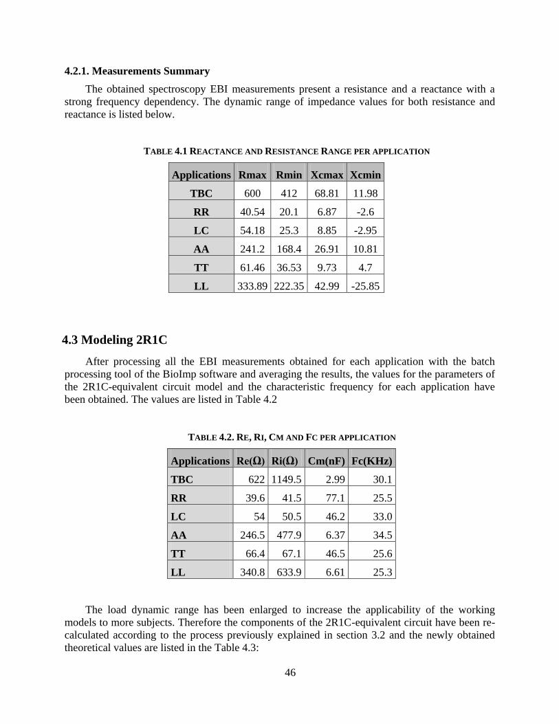
4.2.1. Measurements Summary

The obtained spectroscopy EBI measurements present a resistance and a reactance with a

strong frequency dependency. The dynamic range of impedance values for both resistance and

reactance is listed below.

4.3 Modeling 2R1C

After processing all the EBI measurements obtained for each application with the batch

processing tool of the BioImp software and averaging the results, the values for the parameters of

the 2R1C-equivalent circuit model and the characteristic frequency for each application have

been obtained. The values are listed in Table 4.2

The load dynamic range has been enlarged to increase the applicability of the working

models to more subjects. Therefore the components of the 2R1C-equivalent circuit have been re-

calculated according to the process previously explained in section 3.2 and the newly obtained

theoretical values are listed in the Table 4.3:

TABLE 4.1 REACTANCE AND RESISTANCE RANGE PER APPLICATION

Applications Rmax Rmin Xcmax Xcmin

TBC 600 412 68.81 11.98

RR 40.54 20.1 6.87 -2.6

LC 54.18 25.3 8.85 -2.95

AA 241.2 168.4 26.91 10.81

TT 61.46 36.53 9.73 4.7

LL 333.89 222.35 42.99 -25.85

TABLE 4.2. RE, RI, CM AND FC PER APPLICATION

Applications Re(Ω) Ri(Ω) Cm(nF) Fc(KHz)

TBC 622 1149.5 2.99 30.1

RR 39.6 41.5 77.1 25.5

LC 54 50.5 46.2 33.0

AA 246.5 477.9 6.37 34.5

TT 66.4 67.1 46.5 25.6

LL 340.8 633.9 6.61 25.3

47

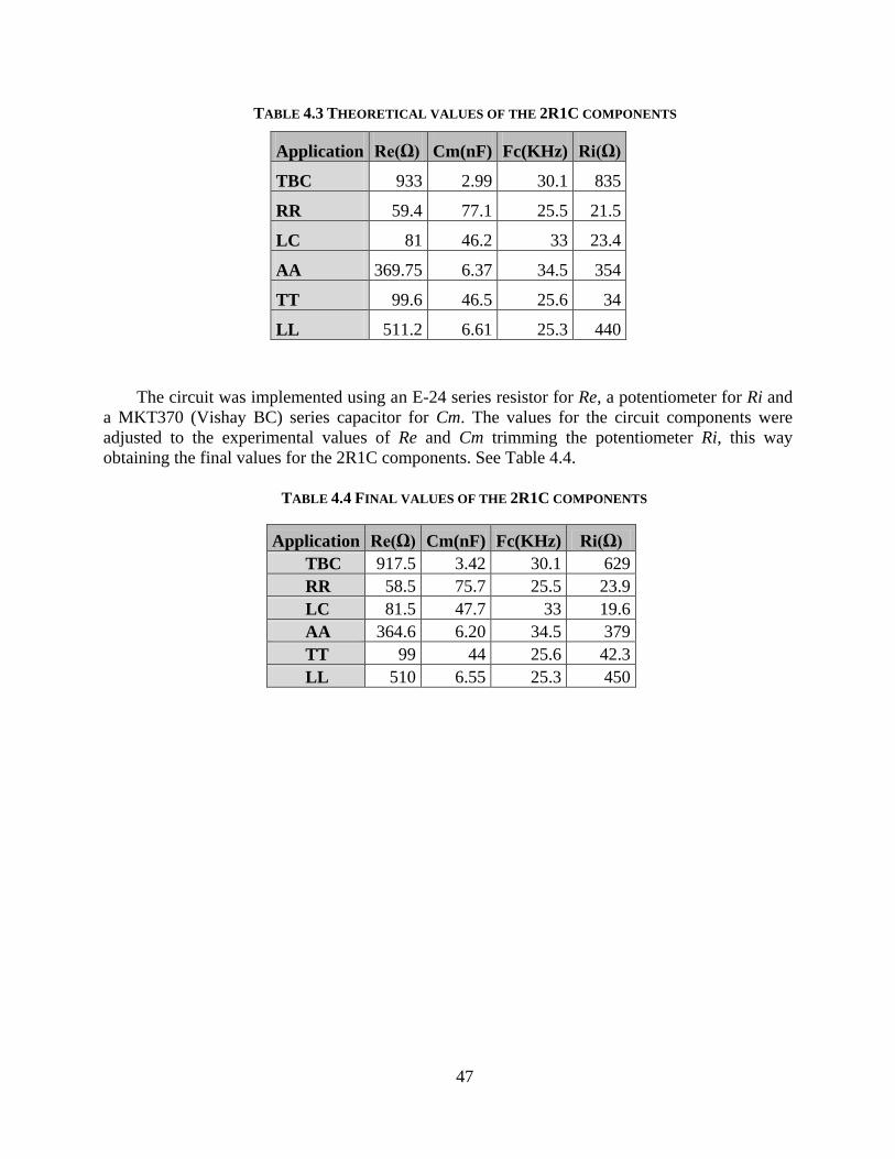
The circuit was implemented using an E-24 series resistor for Re, a potentiometer for Ri and

a MKT370 (Vishay BC) series capacitor for Cm. The values for the circuit components were

adjusted to the experimental values of Re and Cm trimming the potentiometer Ri, this way

obtaining the final values for the 2R1C components. See Table 4.4.

TABLE 4.3 THEORETICAL VALUES OF THE 2R1C COMPONENTS

Application Re(Ω) Cm(nF) Fc(KHz) Ri(Ω)

TBC 933 2.99 30.1 835

RR 59.4 77.1 25.5 21.5

LC 81 46.2 33 23.4

AA 369.75 6.37 34.5 354

TT 99.6 46.5 25.6 34

LL 511.2 6.61 25.3 440

TABLE 4.4 FINAL VALUES OF THE 2R1C COMPONENTS

Application Re(Ω) Cm(nF) Fc(KHz) Ri(Ω)

TBC 917.5 3.42 30.1 629

RR 58.5 75.7 25.5 23.9

LC 81.5 47.7 33 19.6

AA 364.6 6.20 34.5 379

TT 99 44 25.6 42.3

LL 510 6.55 25.3 450

48

4.4. Spectroscopy Measurements in 2R1C Models

Once the equivalents electrical circuits and the optimization of AD5933+4E-AFE have been

already done, the impedance measurements for each model were made by both, the device SFB7

and the AD5933+4E-AFE. The obtained measurements with each of the spectrometers for each

application are shown in the follow figures.

4.4.1 TBC:

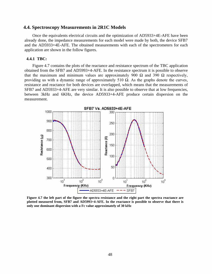
Figure 4.7 contains the plots of the reactance and resistance spectrum of the TBC application

obtained from the SFB7 and AD5993+4-AFE. In the resistance spectrum it is possible to observe

that the maximum and minimum values are approximately 900 Ω and 390 Ω respectively,

providing us with a dynamic range of approximately 510 Ω. As the graphs denote the curves,

resistance and reactance for both devices are overlapped, which means that the measurements of

SFB7 and AD5933+4-AFE are very similar. It is also possible to observe that at low frequencies,

between 3kHz and 6KHz, the device AD5933+4-AFE produce certain dispersion on the

measurement.

Figure 4.7 the left part of the figure the spectra resistance and the right part the spectra reactance are

plotted measured from, SFB7 and AD5993+4-AFE. In the reactance is possible to observe that there is

only one dominant dispersion with a Fc value approximately of 30 kHz

49

4.4.2 RR:

In Figure 4.8 the reactance and resistance spectra of the TBC application for SFB7 and

AD5993+4-AFE are plotted. In the resistance curve is possible to observe that the maximum and

minimum values are approximately 57 Ω and 16 Ω respectively, providing us with a dynamic

range of approximately 41 Ω. As the graphs denote the curves, resistance and reactance for the

both devices are overlapped, therefore it means that the measurements of SFB7 and AD5933+4-

AFE are very similar. It is also possible to observe that at low frequencies, between 3kHz and

6KHz, the measurements performed with the device AD5933+4-AFE present a dispersion.

4.4.3 LC:

In Figure 4.9 the reactance and resistance spectra of the TBC application for SFB7 and

AD5993+4-AFE are plotted. In the resistance curve is possible to observe that the maximum and



both devices are overlapped, therefore it means that the measurements of SFB7 and AD5933+4-

AFE are very similar. It is also possible to observe that at low frequencies, between 3KHz and



plotted measured from both, SFB7 and AD5993+4-AFE. In the reactance is possible to observe that there

is only one dominant dispersion with a Fc value approximately of 27 kHz

50

4.4.4 AA:

In the Figure 4.10 is plotted the reactance and resistance of the TBC application for SFB7

and AD5993+4-AFE.


plotted measured from both, SFB7 and AD5993+4-AFE. In the reactance is possible to observe that

there is only one dominant dispersion with a Fc value approximately of 35 kHz


plotted measured from both, SFB7 and AD5993+4-AFE. In the reactance is possible to observe that

there is only one dominant dispersion with a Fc value approximately of 35 kHz

51

In the resistance curve is possible to observe that the maximum and minimum values are

approximately 365 Ω and 185 Ω respectively, providing us with a dynamic range of

approximately 180 Ω. As the graphs denote the curves, resistance and reactance for the both

devices are overlapped; therefore it means that the measurements of SFB7 and AD5933+4-AFE

are very similar. It is also possible to observe that at low frequencies, between 3kHz and 6KHz,

the measurements performed with the device AD5933+4-AFE present a dispersion.

4.4.5 LL:


and AD5993+4-AFE. In the resistance curve is possible to observe that the maximum and



both devices are overlapped; therefore it means that the measurements of SFB7 and AD5933+4-

AFE are very similar. It is also possible to observe that at low frequencies, between 3KHz and


4.4.6 TT:


and AD5993+4-AFE.


plotted measured from both, SFB7 and AD5993+4-AFE. In the reactance is possible to observe that there

is only one dominant dispersion with a Fc value approximately of 25 kHz

52

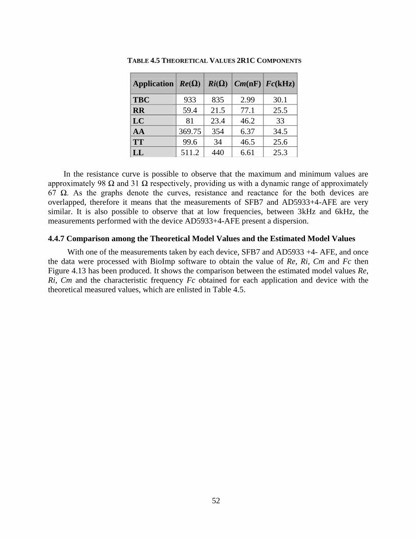
In the resistance curve is possible to observe that the maximum and minimum values are

approximately 98 Ω and 31 Ω respectively, providing us with a dynamic range of approximately

67 Ω. As the graphs denote the curves, resistance and reactance for the both devices are

overlapped, therefore it means that the measurements of SFB7 and AD5933+4-AFE are very

similar. It is also possible to observe that at low frequencies, between 3kHz and 6kHz, the

measurements performed with the device AD5933+4-AFE present a dispersion.

4.4.7 Comparison among the Theoretical Model Values and the Estimated Model Values

With one of the measurements taken by each device, SFB7 and AD5933 +4- AFE, and once

the data were processed with BioImp software to obtain the value of Re, Ri, Cm and Fc then

Figure 4.13 has been produced. It shows the comparison between the estimated model values Re,

Ri, Cm and the characteristic frequency Fc obtained for each application and device with the

theoretical measured values, which are enlisted in Table 4.5.

TABLE 4.5 THEORETICAL VALUES 2R1C COMPONENTS

Application Re(Ω) Ri(Ω) Cm(nF) Fc(kHz)

TBC 933 835 2.99 30.1

RR 59.4 21.5 77.1 25.5

LC 81 23.4 46.2 33

AA 369.75 354 6.37 34.5

TT 99.6 34 46.5 25.6

LL 511.2 440 6.61 25.3

53

In Figure 4.13 it is possible to observe the calculated value and the obtained value from the

measurements of both devices are quite similar, the maximum difference is in the value of Ri,

between the calculated value and obtained value from the devices in the TBC application.

4.5. SFB7 Vs. AD5933+4-AFE

In order to show the performance comparison between the SFB7 and the AD5933+4-AFE

the following statistical parameters were chosen:

- Absolute and Relative Error

- Average

- Standard deviation

- Maximum and Minimum

Figure 4.13 This graph shows in a) the membrane capacitance, in b) the intracellular resistance, in c) the

extracellular Resistance and in d) the characteristic frequency per each application and measured with,

both devices the SFB7 and AD5933+4-AFE, and also the theoretical value calculated.

54

Therefore, with all the measurements already processed with BioImp software, all the

estimation results were exported to a MS Excel file. Once all the data were exported to MS Excel,

the statistical values were calculated with the statistical tools available within MS Excel. Firstly,

the absolute and relative error comparisons between SFB7 and AD5933+4-AFE were done.

Figure 4.14 and 4.15 show both errors.

Figure 4.14 Relative error of Ri, Re, Cm and Fc for each application and device: SFB7 and AD5933+4-AFE.

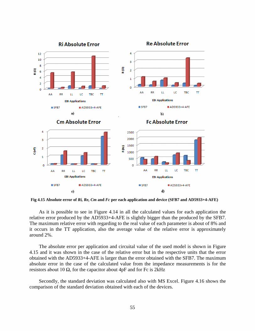
55

As it is possible to see in Figure 4.14 in all the calculated values for each application the

relative error produced by the AD5933+4-AFE is slightly bigger than the produced by the SFB7.

The maximum relative error with regarding to the real value of each parameter is about of 8% and

it occurs in the TT application, also the average value of the relative error is approximately

around 2%.

The absolute error per application and circuital value of the used model is shown in Figure

4.15 and it was shown in the case of the relative error but in the respective units that the error

obtained with the AD5933+4-AFE is larger than the error obtained with the SFB7. The maximum

absolute error in the case of the calculated value from the impedance measurements is for the

resistors about 10 Ω, for the capacitor about 4pF and for Fc is 2kHz

Secondly, the standard deviation was calculated also with MS Excel. Figure 4.16 shows the

comparison of the standard deviation obtained with each of the devices.

Fig 4.15 Absolute error of Ri, Re, Cm and Fc per each application and device (SFB7 and AD5933+4-AFE)

56

Although the relative error obtained with the AD5933+4-AFE is most of the time larger

than the error obtained with the SFB7, as shown in Figure 4.15, the standard deviation of the

SFB7 is larger than the standard deviation produced by the AD5933+4-AFE in all the circuital

values calculated in each of the applications.

Finally in Matlab, the average, maximum, minimum of the estimated values and the real

value of the component of each EBI model application have been plotted on Figures 4.17, 4.18,

4.19, 4.20, 4.21 and 4.22.

Figure 4.16 Standard deviation of Ri, Re, Cm for each application and impedance spectrometer device:

SFB7 and AD5933+4-AFE.

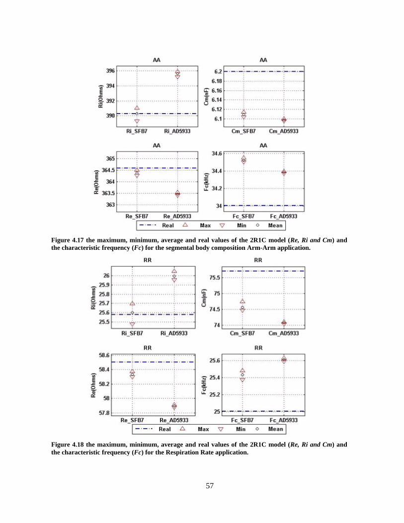
57

Figure 4.17 the maximum, minimum, average and real values of the 2R1C model (Re, Ri and Cm) and

the characteristic frequency (Fc) for the segmental body composition Arm-Arm application.

Figure 4.18 the maximum, minimum, average and real values of the 2R1C model (Re, Ri and Cm) and

the characteristic frequency (Fc) for the Respiration Rate application.

58

Figure 4.19 the maximum, minimum, average and real values of the 2R1C model (Re, Ri and Cm) and the

characteristic frequency (Fc) for the segmental body composition Leg-Leg Application.


characteristic frequency (Fc) for the Lungs Composition application.

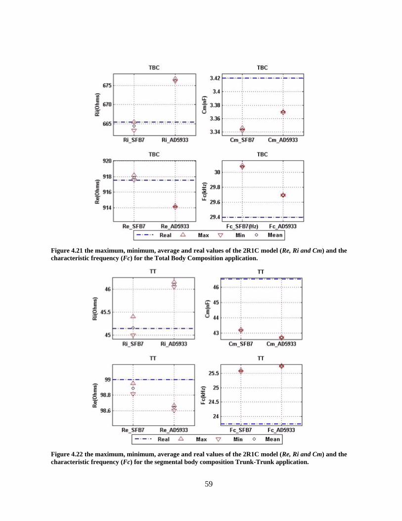
59


characteristic frequency (Fc) for the Total Body Composition application.


characteristic frequency (Fc) for the segmental body composition Trunk-Trunk application.

60

The previous figures show the maximum, minimum, average and real values for the 2R1C

model and it is possible to see that in almost in all the EBI applications, the SFB7 produces a

closer value to the real values of the of the 2R1C models than the values estimated with the

AD5933+4-AFE measurements, as shown in Figure 4.14 and Figure 4.15, the relative error and

the absolute error respectively. In addition the Figures show with the indicators of the maximums

and minimums that the dispersion of estimations produced by the SFB7 measurements is larger

than the estimations produced with the AD5933+4-AFE measurements as shown in Figure 4.16.

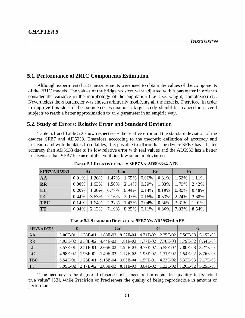
61

CHAPTER 5

DISCUSSION

5.1. Performance of 2R1C Components Estimation

Although experimental EBI measurements were used to obtain the values of the components

of the 2R1C models. The values of the bridge resistors were adjusted with α parameter in order to

consider the variance in the morphology of the population like size, weight, complexion etc.

Nevertheless the α parameter was chosen arbitrarily modifying all the models. Therefore, in order

to improve this step of the parameters estimation a target study should be realized in several

subjects to reach a better approximation to an α parameter in an empiric way.

5.2. Study of Errors: Relative Error and Standard Deviation

Table 5.1 and Table 5.2 show respectively the relative error and the standard deviation of the

devices SFB7 and AD5933. Therefore according to the theoretic definition of accuracy and

precision and with the dates from tables, it is possible to affirm that the device SFB7 has a better

accuracy than AD5933 due to its low relative error with real values and the AD5933 has a better

preciseness than SFB7 because of the exhibited low standard deviation.

“The accuracy is the degree of closeness of a measured or calculated quantity to its actual

true value” [33], while Precision or Preciseness the quality of being reproducible in amount or

performance.

TABLE 5.2 STANDARD DEVIATION: SFB7 VS. AD5933+4-AFE

SFB7/AD5933 Ri Cm Re Fc

AA 3.06E-01 1.33E-01 1.88E-03 9.57E-04 4.71E-02 2.35E-02 7.56E-03 5.15E-03

RR 4.93E-02 2.38E-02 4.44E-02 1.81E-02 1.77E-02 7.70E-03 1.79E-02 8.54E-03

LL 3.57E-01 2.21E-01 2.66E-03 1.92E-03 9.77E-02 5.55E-02 7.80E-03 3.27E-03

LC 4.98E-02 1.93E-02 1.49E-02 1.17E-02 1.93E-02 1.31E-02 1.54E-02 8.76E-03

TBC 5.54E-01 1.28E-01 9.15E-04 3.05E-04 1.59E-01 4.23E-02 5.32E-03 2.17E-03

TT 7.99E-02 2.17E-02 2.03E-02 8.11E-03 3.04E-02 1.22E-02 1.26E-02 5.25E-03

TABLE 5.1 RELATIVE ERROR: SFB7 VS. AD5933+4-AFE

SFB7/AD5933 Ri Cm Re Fc

AA 0.01% 1.36% 1.47% 1.65% 0.06% 0.31% 1.52% 1.11%

RR 0.08% 1.63% 1.50% 2.14% 0.29% 1.03% 1.70% 2.42%

LL 0.20% 1.20% 0.78% 0.94% 0.14% 0.19% 0.80% 0.48%

LC 0.44% 3.63% 2.16% 2.97% 0.16% 0.53% 2.24% 2.68%

TBC 0.14% 1.64% 2.22% 1.47% 0.04% 0.36% 2.31% 1.01%

TT 0.04% 2.13% 7.19% 8.25% 0.11% 0.36% 7.82% 8.54%

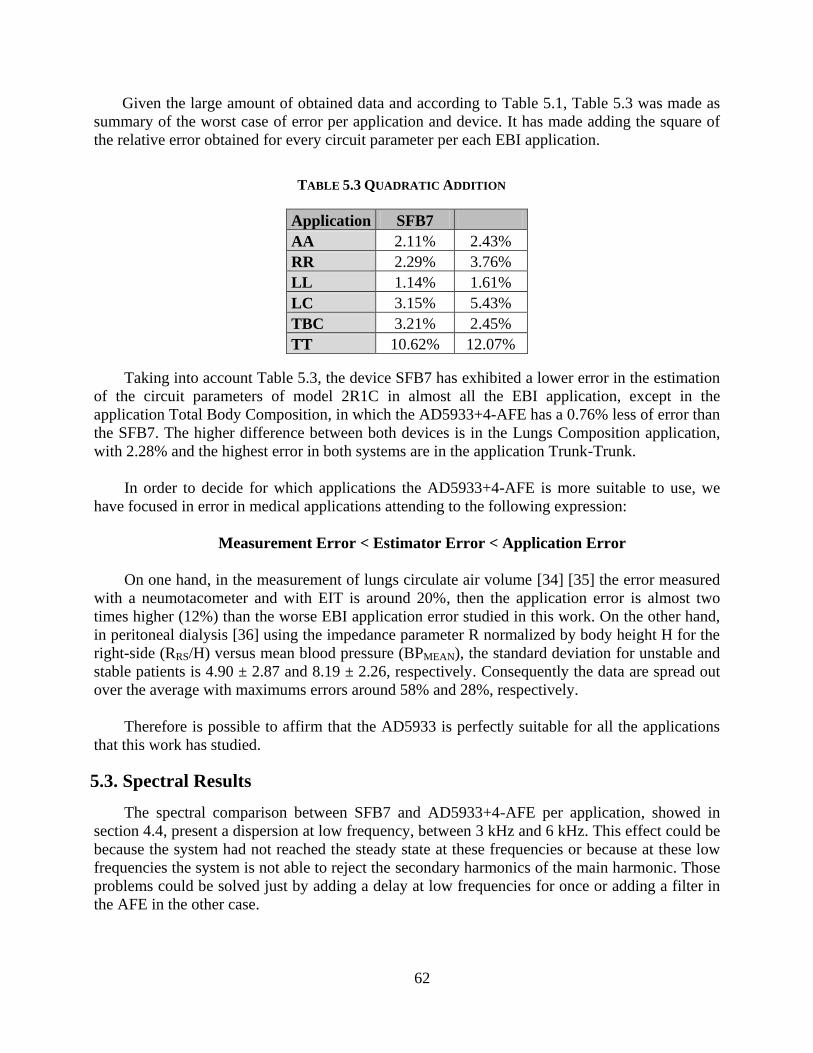
62

Given the large amount of obtained data and according to Table 5.1, Table 5.3 was made as

summary of the worst case of error per application and device. It has made adding the square of

the relative error obtained for every circuit parameter per each EBI application.

Taking into account Table 5.3, the device SFB7 has exhibited a lower error in the estimation

of the circuit parameters of model 2R1C in almost all the EBI application, except in the

application Total Body Composition, in which the AD5933+4-AFE has a 0.76% less of error than

the SFB7. The higher difference between both devices is in the Lungs Composition application,

with 2.28% and the highest error in both systems are in the application Trunk-Trunk.

In order to decide for which applications the AD5933+4-AFE is more suitable to use, we

have focused in error in medical applications attending to the following expression:

Measurement Error < Estimator Error < Application Error

On one hand, in the measurement of lungs circulate air volume [34] [35] the error measured

with a neumotacometer and with EIT is around 20%, then the application error is almost two

times higher (12%) than the worse EBI application error studied in this work. On the other hand,

in peritoneal dialysis [36] using the impedance parameter R normalized by body height H for the

right-side (RRS/H) versus mean blood pressure (BPMEAN), the standard deviation for unstable and

stable patients is 4.90 ± 2.87 and 8.19 ± 2.26, respectively. Consequently the data are spread out

over the average with maximums errors around 58% and 28%, respectively.

Therefore is possible to affirm that the AD5933 is perfectly suitable for all the applications

that this work has studied.

5.3. Spectral Results

The spectral comparison between SFB7 and AD5933+4-AFE per application, showed in

section 4.4, present a dispersion at low frequency, between 3 kHz and 6 kHz. This effect could be

because the system had not reached the steady state at these frequencies or because at these low

frequencies the system is not able to reject the secondary harmonics of the main harmonic. Those

problems could be solved just by adding a delay at low frequencies for once or adding a filter in

the AFE in the other case.

TABLE 5.3 QUADRATIC ADDITION

Application SFB7

AA 2.11% 2.43%

RR 2.29% 3.76%

LL 1.14% 1.61%

LC 3.15% 5.43%

TBC 3.21% 2.45%

TT 10.62% 12.07%

63

As it was possible to see on the spectral plots for each application the continuous blue line

representing the measurements obtained with the AD5933+4-AFE follow accurately the

discontinuous red line representing the measurements taken with the SFB7, in both resistance and

reactance. Whereupon the spectroscopy measurements performance exhibited by the AD5933+4-

AFE it is possible to conclude that the device will be suitable for the applications under study.

64

CHAPTER 6

CONCLUSIONS & FUTURE WORK

6.1. Conclusions

After all the results shown in the chapter 4 and discussion in chapter 5, it can be concluded

that the combination AD5933+4-AFE is suitable to realize spectroscopy measurements of the

EBI applications studied in this master thesis. This result has significant repercussions as in

economic terms due to the high integration of AD5933 (I2C interface, DDS, Amplifiers, PGA,

Low pass Filter, ADC, DSP and Temperature sensor) as in the electronic instrumentation because

it opens up new horizons for the integration of the measurement systems of EBI into portable and

even wearable systems.

6.2. Future work

Once the main target of this work has been done, with the aim to solve some problems or to

improve the applied method and the system AD5933+4-AFE the next points has brought up:

The α parameter was chosen arbitrarily and due to it all the models have been

affected. Therefore, in order to improve this step in the estimation a study in several

subjects should be realized to reach better approximation to α parameter by empiric

way.

The frequency distribution of measurements performed by the SFB7 and AD5933+4-

AFE is exponential and linear, respectively. With the goal of improving the

comparison between both devices, it will be better to change by software the

frequency distribution of the AD5933.

To use resistors and capacitors with a low tolerance, in order to obtain a lower

variability between the models measurements

To add a larger delay at low frequencies or adding a filter in the AFE to reduce de

dispersion at low frequencies.

Due to the spectral variability of the impedance under study in each application and

to make suitable the combination AD5933+4-AFE for many applications, it will be a

good improvement to add a differential PGA (Programmable Gain Amplifier) or

scalable resistors array.

65

REFERENCES

[1] S. Grimnes and Ø. G. Martinsen, Bioimpedance & Bioelectricity Basics: Academic Press,

2000.

[2] A. Piccoli, B. Rossi, L. Pillon, and G. Bucciante, "A new method for monitoring body

fluid variation by bioimpedance analysis: the RXc graph," 1994.

[3] F. Seoane, "Electrical Bioimpedance Cerebral Monitoring: Fundamental Steps towards

Clinical Application," in Signal & Systems. vol. PhD Göteborg: Chalmers University of

Technology, 2007, p. 154.

[4] M. Phillippson, "Les Lois De La Resistance Electrique Des Tissus Vivants," Bull. Acad. roy.

Belgique, 1921.

[5] H. Fricke, "A Mathematical Treatment of the Electrical conductivity of Colloids and Cell

Suspensions," Journal of General Physiology, pp. 375-383, Jan 4 1924.

[6] K. S. Cole, "Electric impedance of suspensions of spheres," Journal of General

Physiology, vol. 12, pp. 29-36, 1928.

[7] J. Nyboer, S. Bango, A. Barnett, and R. H. Halsey, "Radiocardiograms: Electrical

impedance changes of the heart in relation to electrocardiograms and heart sounds," J.

Clin. Invest., vol. 19, p. 773, 1940.

[8] T. Olsson and L. Victorin, "Transthoracic impedance, with special reference to newborn

infants and the ratio air-to-fluid in the lungs," Acta Paediatr Scand Suppl, vol. 207, p.

Suppl 207:1ff, 1970.

[9] R. F. Kushner and D. A. Schoeller, "Estimation of total body water by bioelectrical

impedance analysis," Am J Clin Nutr, vol. 44, pp. 417-24, Sep 1986.

[10] P. Aberg, I. Nicander, J. Hansson, P. Geladi, U. Holmgren, and S. Ollmar, "Skin cancer

identification using multifrequency electrical impedance – A potential screening tool,"

IEEE Trans. Bio. Med. Eng., vol. 51, pp. 2097-2102, 2004.

[11] H. P. Schwan, "Electrical properties of tissue and cell suspensions," Adv Biol Med Phys,

vol. 5, pp. 147-209, 1957.

[12] H. Morel and M. Y. Jaffrin, "Total body water measurement: using the multifrequency

BIS-Hanai approach with 50 kHz single frequency," in 13th International Conference on

Electrical Bioimpedance and the 8th Conference on Electrical Impedance Tomography,

2007, pp. 799-802.

[13] A. De Lorenzo, A. Andreoli, J. Matthie, and P. Withers, "Predicting body cell mass with

bioimpedance by using theoretical methods: a technological review," J Appl Physiol, vol.

82, pp. 1542-58, May 1997.

[14] U. Kyle, I. Bosaeus, A. D. De Lorenzo, P. Deurenberg, M. Elia, J. M. Gomez, B. L.

Heitmann, L. Kent-Smith, J. Melchior, M. Pirlich, H. Scharfetter, A. M. W. J. Schols, and

C. Pichard, "Bioelectrical impedance analysis--part I: review of principles and methods,"

2004.

[15] M. Y. Jaffrin and H. Morel, "Body fluid volumes measurements by impedance: A review

of bioimpedance spectroscopy (BIS) and bioimpedance analysis (BIA) methods," Medical

Engineering & Physics, vol. 30, pp. 1257-1269, 2008.

[16] G. B. Forbes, Human body composition : growth, aging, nutrition, and activity / Gilbert

B. Forbes: Springer-Verlag, 1987.

66

[17] F. J. Deurenberg P Fau - Schouten and F. J. Schouten, "Loss of total body water and

extracellular water assessed by multifrequency impedance."

[18] U. G. Kyle, I. Bosaeus, A. D. De Lorenzo, P. Deurenberg, M. Elia, J. M. Gomez, B. L.

Heitmann, L. Kent-Smith, J. C. Melchior, M. Pirlich, H. Scharfetter, A. M. W. J. Schols,

and C. Pichard, "Bioelectrical impedance analysis--part I: review of principles and

methods," Clin Nutr, vol. 23, pp. 1226-43, Oct 2004.

[19] R. Patel, E. L. Peterson, N. Silverman, and B. J. Zarowitz, "Estimation of total body and

extracellular water in post-coronary artery bypass graft surgical patients using single and

multiple frequency bioimpedance," 1996.

[20] W. Hannan, S. J. Cowen, C. E. Plester, K. C. Fearon, and A. Beau, "Comparison of bio-

impedance spectroscopy and multi-frequency bio-impedance analysis for the assessment

of extracellular and total body water in surgical patients," 1995.

[21] K. S. Cole, "Permeability and impermeability of cell membranes for ions.," Quant. Biol.,

vol. 8, pp. 110–122, 1940.

[22] T. Hanai, N. Koizumi, and R. Gotoh, "Dielectric properties of emulsions," Colloid &

Polymer Science, vol. 184, pp. 143-148, 1962.

[23] P. Nopp, N. Harris, T. Zhao, and B. Brown, "Model for the dielectric properties of human

lung tissue against frequency and air content," Medical and Biological Engineering and

Computing, vol. 35, pp. 695-702, 1997.

[24] L. A. Baker Le Fau - Geddes, H. E. Geddes La Fau - Hoff, C. J. Hoff He Fau - Chaput,

and C. J. Chaput, "Physiological factors underlying transthoracic impedance variations in

respiration."

[25] L. E. Baker, L. A. Geddes, and H. E. Hoff, "quantitative evaluation of impedance

spirometry in man," The American journal of medical electronics, 1965.

[26] A. F. Pacela, "Impedance pneumography--a survey of instrumentation techniques."

[27] A. Fein, R. F. Grossman, J. G. Jones, P. C. Goodman, and J. F. Murray, "Evaluation of

transthoracic electrical impedance in the diagnosis of pulmonary edema," Circulation,

1979.

[28] F. Larsen, L. Mogensen, and B. Tedner, "Transthoracic electrical impedance at 1 and 100

kHz--a means for separating thoracic fluid compartments?," Clinical Physiology, 1987.

[29] F. Seoane, J. Ferreira, J. J. Sanchéz, and R. Bragós, "Analog Front-End Enables Electrical

Impedance Spectroscopy System On-Chip for Biomedical Applications," Physiol. Meas. ,

vol. 29 pp. S267-S278, 2008.

[30] H. Fricke and S. Morse, "The Electric Resistance and Capacity of Blood for Frequencies

Between 800 and 4.5 Million Cycles," Journal of General Physiology, vol. 9, pp. 153-67,

1925.

[31] J. Ferreira and J. J. Sanchez, "Electrical Bioimpedance Measurement System for Limb

Edema Monitoring," in School of Engineering. vol. MSc Borås: University College of

Borås, 2007, p. 104.

[32] H. Scharfetter, P. Hartinger, H. Hinghofer-Szalkay, and H. Hutten, "A model of artefacts

produced by stray capacitance during whole body or segmental bioimpedance

spectroscopy," Physiological Measurement, vol. 19, pp. 247-261, 1998.

[33] J. Taylor, An Introduction to Error Analysis: University Science Books, 1997.

[34] M. Balleza, N. Calaf, T. Feixas, M. González, D. Antón, P. J. Riu, and P. Casan,

"Medición del patrón ventilatorio mediante tomografía por impedancia eléctrica en

pacientes con EPOC " Archivos de bronconeumología, vol. 45 núm. 07, pp. 320-324,

2009.

67

[35] M. Balleza, J. Fornos, N. Calaf, T. Feixas, M. González, D. Antón, P. J. Riu, and P.

Casan, "Seguimiento del patrón ventilatorio en reposo mediante tomografía por

impedancia eléctrica " Archivos de Bronconeumología, vol. 43, núm 6, pp. 300-303, 2007.

[36] L. Nescolarde, J. Rosell, and T. Doñate, "Relationship between segmental and whole-

body phase angle in peritoneal dialysis patients," Physiological Measurement, vol. 29, p.

N49, 2008.

Documents

Final Degree Thesis - UPCommons Degree... · Final Degree Thesis A Feasibility Study of the Suitability of an AD5933-based Spectrometer for EBI Applications By Antonio Ansede Pena