Embed Size (px)
Citation preview

FIELD THEORY ANALYSIS OF RECTANG ULAR A N D CIRCULAR W AVEGUIDE DISCO NTINUITIES FOR FILTERS, M ULTIPLEXERS A N D M ATCH ING
NETW O RK Sby
Benoît Varailhon de la Filolie
Maître es science, 1984 (Université de Bordeaux, France)Diplômé Ingénieur INSA, 1987 (INSA Rennes, France)
A DISSERTATION SUBMITTED IN PARTIAL FULFILLMENT OF THE REQUIREMENTS FOR THE DEGREE OF
A C C E P T E D DOCTOR OF PHILOSOPHYA C U L T w T y A B W A ^ T U D I E S
We accept this dissertation as conforming Wthc/reqaired standard
— jDr. R. Vahldieclu Supervisor & Graduate Advisor, Dept, of Elect. Sz Comp. Eng.
Dr. ,1. Borncmann, Department Member, Dept, of Elect. &: Comp. Eng.
Dr. P. F. Friessen, Department Member, Dept, of Elect. & Comp. Eng.
___________________
Dr. R. N. Horspool, Outside Member, Dept, of Computer Science
Dr. B. Tabarrok, Outsidc^Ji^gmber, Dept, of Mechanical Engineering
r. V . K. IH n a tn i , E x WDr. V. R Trjpafrii, P.vfprnal Fviinînor Oregon State University
©Benoît Varailhon de la FILOLIE, 1992UNIVERSITY OF VICTORIA
AU rights reserved. This dissertation may not be reproduced in whole or in part, by photocopy or other means,
without the permission of the author.

SupcrvÎKor: Dr. R. Vîihldicck
ABSTRACT
Progress in întegraUng microwave circnlls depends largely on the development
of computationally effective and accurate numerical m ethods. These methods allow a
miniaturization of microwave components and their utilization at higher frequency.
In this thesis, the a])plicatlon of the mode matching method Is described as well as
their modification to different kinds of structure in rectangular and circular waveguides.
The task is to design and optimize filters, multiplexers and impedance matching net
works. In its most general form, the mode matching method a t waveguide discontinuities
requires the matching of four field components. However, to Improve computational ef
ficiency, the effect of matching only two field components (versus four field components)
is Investigated and successfully exploited for selected discontinuities.
To satisfy space requirements, low loss, compact, and lightweight dlplcxer, triplexer
and qiiadriplexcr structures in rectangular waveguide technology are designed and op
timized. The analysis Is made possible by decomposing the structu re Into simple dis
continuity sections such as discontinuity in width, height or bl- and tri-furcatlons.
Three different types of discontinuities In coaxial waveguide are investigated: the
outer stop, the Inner step and the gap discontinuities. By cascading such discontinuities,
filters or matching networks can be obtained.
Finally, a new typo of circular waveguide bandpass filter using printed metal Inserts
is developed and designed in Ka-band. A comparison between theoretical results and
measurements shows excellent agreement.

Examiners:
Dr. R. Vahldicclw^Supervisor & G raduate Advisor, Dept, of Elect. & Comp. Eng.
Dr. J . Boriiemann, Departm ent Member, Dept, of Elect. & Comp. Eng.
Dr. P. F . Friessen, D epartm ent Member, Dept, of Elect. & Comp. Eng.
________
Dr. R. N. Horspool, Outside Member, Dept, of Com puter Science
Dr. B. Tabarrok, Outside M ember, Dept, of Mechanical Engineering
Dr. V. K. Tripathi, External Examiner, Oregon S tale University
111

IV
Table o f C ontents
A bstract ii
Table o f C ontents îv
List o f Tables viil
List o f Figures ixr
Acknowledgem ent xiii
1 Introduction 1
1.1 Numerical m ethods - an overv iew ........................................................................ 6
1.2 The Mode M atching M ethod .............................................................................. 9
1.2.1 Theoretical foundation of the M M M ................................................... 9
2 Parallel-connected diplexer 13
2.1 Vector p o te n tia l............................................................................................................ 16
2.2 Matching c o n d itio n ...................................................................................... . . . 18
2.2.1 M atching the electric f ie ld ........................................................................ 18
2.2.2 M atching the magnetic f ie ld ..................................................................... 19

TAULE OF CONTENTS V
2.2.3 E-platic b ifu rcation .................................................................................... 2(1
2.3 Coiivorgc.ncc an a ly s is .............................................................................................. 22
2.'I Power d iv id e r ......................................................................................................... 23
2.5 Diple.xer-lVi plexor ................................................................................................. 2(i
2.5.1 D ip lexer......................................................................................................... 2(1
2.5.2 Double band-pass filter ................. ■....................................................... 30
2.5.3 Triplexer ..................................................................................................... 30
3 D o u b le -s te p d isc o n tin u itie s 30
3.1 TE'^ approach ............... 37
3.2 Full wave analysis ................................................................................................. dO
3.2.1 Matching equation ......................................................................... <12
3.2.2 Comparison of both a])proaches..................................................... dd
3.3 Alternative a p p ro ach ................... d(i
3.d Application to power divider and (;uadrlplexor ........................................... dS
4 C o a x ia l c irc u la r w avegu ide 51
4.1 Vector p o ten tia l...................... 52
4.2 Inner s t e p ................................................................................................................. 57
4.3 R esu lts ............................................. 58
4.3.1 Convergence an a ly s is ......................................................... 58
4.3.2 Stop discontinuities.................................................................................... 58
4.3.3 Very low-roturn-loss adapter ................................................................ GI
4.3.4 Coaxial f ille rs .............................................................................................. 03

TAULE o r CO NTENTS vl
A A Fillers witii gap .............................................................................................. 67
'1.4.1 Analysis of liie coaxial gap (liscoiitim iily ............................................... 67
4.4.2 RestilLs ............................................................................ 70
5 M e ta l- in s e r t c irc u la r w av eg u id e f il te r 75
5.1 Potential c ()nations.................................................. 77
5 .1.1 tf-ccpiation ............................................................................................. 78
5.1.2 />-e<piatioii . . 1 . . . . . . ................................................................. 80
5.2 Field expressions ................ 80
5.8 Matching equations ....................................................................................... 82
5.3.1 First coupling equation .................................. 82
5.3.2 Remaining coupling eq u a tio n s .................................................................. 85
5.4 Scattering M atrix of the discontinuity ................................................. 86
5.5 Convergence a n a ly s is ................................ 89
5.6 Bandpjiss f ilte rs ........................................................................................................ 89
5.7 Coaxial bow-tie shaped d isco n tin u ity .................. 95
5.8 Bandpass filter .............................................................................................. 102
6 C o nc lu sion 105
6.1 R esu lts .............................................................. 105
6.2 l^irthcr work . ..................................................................................................... 106
A F ro m th e coup ling m a tr ic e s to th e s c a t te r in g m a tr ix 110
B F ie ld c o m p o n e n ts in coax ia l w av eg u id es 112

TA B L E OF C O N TE N TS vii
C Field expressions in circular waveguides 11 :i
C .l Emply circular w avcgitido ...................................................................................... li;}
C.2 Upper half circular wa.n i id e ..................................................................................... IM
C.3 Ortho-uorinalizaUoii "euI s ........................................................................... 11-1
C.4 Magnetic fie ld ............................................................................................................. llTi
C.5 Normalization cocfncient...................................................................................... 115
D Coupling integrals 117
D.I Second coupling ecpiation ................................................................................... 117
D.2 Third coupling e q u a tio n ...................................................................................... II!)
D.3 Fourth coupling ocpiation ................................................................................... 122
E Full wave expressions in coaxial waveguides 125
E .l Coaxial circular waveguide................................................................................... 125
E.2 Upper sectorial coaxial waveguide...................................................................... !2ti
E.3 Normalization coeffic ien ts ................................................................................... 120
F M athem atical formulae 127
F .l Bessel’s e q u a t io n .......................................................... , ....................................... 127
F.2 Sine integrals................................................................................................. 128
Bibliography 130

VI l i
List o f Tables
1.1 Comparison of durèrent miinorica! n ic t l io d s ............... 8
2.1 Mcclianicui dimensions of the X-band power divider, VV-Band power di
vider, Ka-l)and and VV-band filters.............................................. 34
2.2 Mechanical dimensions of the Ka- and W-band metal insert filters. . . . 35
3.1 Mechanical dimensions of the W-band 4-way power divider and qiiadriplc.xcr. 49
4.1 D ata for an optimized low-return-Ioss adapter................................................ G2
4.2 D ata of the Ka-band bandpass coax filter.................................... G7
4.3 Vailles for the discontinuity capacitance of a 50 0-coaxial guide term i
nated in a circular waveguide................................................................................ 70
4.4 D ata for the optimized gapped 3-soction coaxial filter................................... 73
5.1 Mechanical dimensions of the Ka-band three- and five-resonator circular
waveguide filter......................................................................................................... 98
5.2 Mechanical dimensions of the five-resonator coaxial waveguide filter. . . 103

IX
List o f F igures
1.1 Com|):irisoii hetwcen a) a typical m u l t i p l e . \ o r / ( l o - i i m l l h ) i Ikî pro
posed new .structure and c) its extension to a (pindriplrxer.......................... I
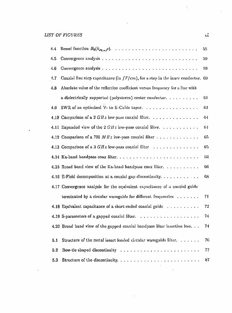
1.2 Example of an arbitrary sliaped d isc o n tin u ity ................................. II
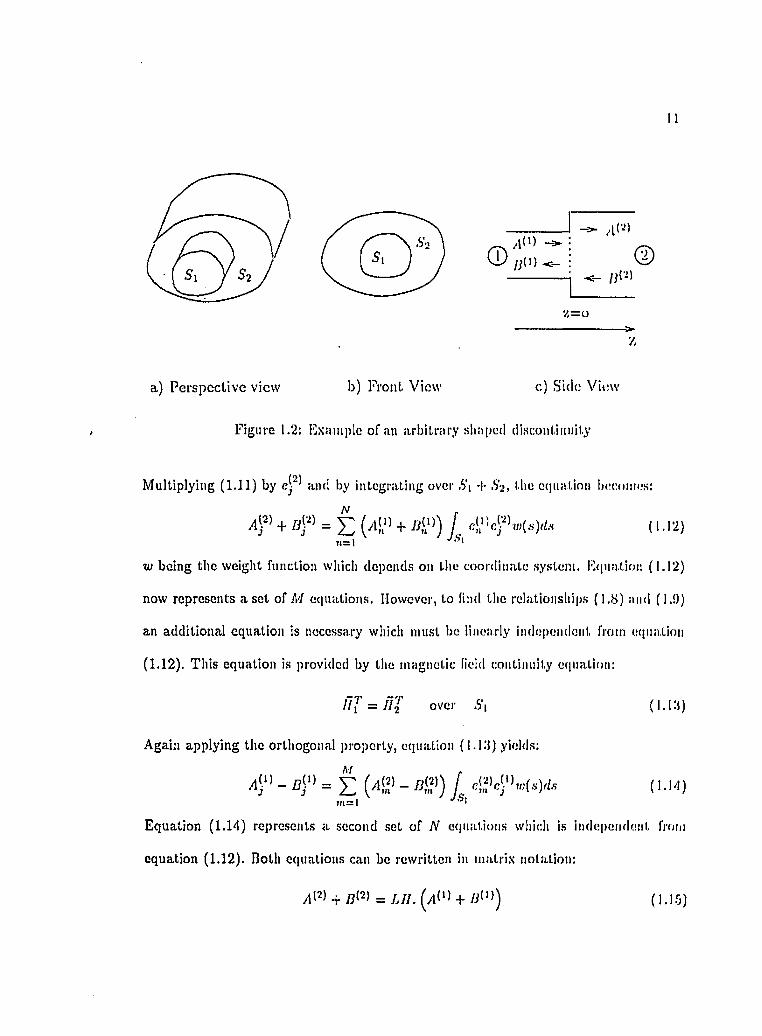
2.1 Mectianical composition of the diplexer................................................ I I
2.2 Decomposition of the diplexer into simple discontinuity eleiinnits.............. I."")
2.3 Side view of an E-plane step discontinuity. . ............................................... ID
2.d Side view of an E-plane bifurcation....................................................... 21
2.5 Convergence analysis of an E-plane step discontinuity and its equivalent
capacitance............................................................................ ... ................................. 23
2.6 Convergence analysis of an E-plane step discontinuity..................... 2-1
2.7 Convergence analysis of an E-plane step discontinuity..................... 21
2.8 Convergence analysis of an E-plane step discontinuity with the freipiency
as param eter..................................................................................................... 2.5
2.9 Convergence analysis for a W -band power divider fed by a ,5-step taper
transition, .................................................................................................... 26
2.10 Frequency response of an optimized tapered X-band power divider. . . . 27
2.11 Frequency response of an optimized tapered W-band power divider. . . 27

LIST OF FKUJIŒS x
2 . 1‘2 Hcliirii loss versus fiü(|U(Uicy for an optimized VV-band 3-clianncl power
divider............................................................................................................... 28
2.13 Insertion loss versus frequency of the different channels of an optimized
VV-IJand 3-channel power divider.............................................................. 28
2.1'I Perspective view of the diplexer arrangem ent with ladder-shaped metal
insert 15-plane filters..................................................................................... 29
2.15 Kreqiiency response of the optimized Ka-band diplexer.................................. 31
2.10 frequency response of the optimized W-band diplexer................................... 31
2.17 Frequency response of an optimized double-band filler.................................. 32
2.18 Fre(|uency response of the optimized VV-band triplexer.................................. 33
3.1 Mechanical composition of the quadriplexer......................................... 37
3.2 Detail of the double step discontinuity.................................................... 38
3.3 M agnitude of the reflection coefficient of a linear Ku-to-X-band trans
former (approximated by 2-1 steps) 45
3.4 Insertion loss of a three-resonator iris-coupled Ku-band waveguide filter 45
3.5 Insertion loss of a. single resonant iris in a Ka-band waveguide....... 47
3.(1 Ueturn loss of a resonant iris in a Ka-band waveguide...................... 47
3.7 Frecjuency response of an optimized 4-channcl power divider........................ 49
3.8 Frequency response of an optimized quadriplexer............................................. 50
4.1 Types of coaxial discontinuities................................................................ 51
4.2 15-field decomposition of an inner step discontinuity........................... 53
4.3 Side view of a coax cable............................................................................ 54
LIST OF FIGURES xi
4.4 Kessel fimcUon J3o(^>o.m/0‘ ............................................................................... 55
4.5 Convergence a n a ly s is ................................................................................... 51)
4.6 Convergence a n a ly s is ................................... 51)
4.7 Coaxial line stop capacitance (lu / / ‘’/cn i) , for a step in tlie inner conductor. 60
4.8 Absolute vaine of the reflection coefficient versus freipiency for a line with
a dielectrically supported (polysteren) center conductor..................... 61
4.1) SW ll of an optimized V- to K-Cable tap e r ...................................................... 6'2
4.10 Comparison of a 2 G I l z low-pass coaxial filler.............................................. 61
4.11 Expanded view of the 2 G H z low-pass coaxial filler....................................... 61
4.12 Comparison of a 700 M I I z low-pass coaxial f i l te r ........................................ 65
4.13 Comparison of a 3 G H z low-pass coaxial filler .............................................. 65
4.14 Ka-band bandpass coax filter............................................................................... 66
4.15 Broad band view of tlie Ka-band bandpass coax filter................................... 66
4.16 E-Field decomposition at a coaxial gap discontinuity . . 68
4.17 Convergence analysis for the equivalent capacitance of a coaxial guide
term inated by a circular waveguide for different fre q u e n c ie s .................... 71
4.18 Equivalent capacitance of a short-ended coaxial guide .............................. 72
4.19 S-paraineters of a gapped coaxial filter............................................................... 74
4.20 Broad band view of the gapped coaxial bandpass filler insertion loss. . . 74
5.1 Structure of the metal insert loaded circular waveguide filter...................... 76
5.2 Bow-tie shaped discontinuity ............................................................................. 77
5.3 S tructure of the discontinuity.................................... 87

LIST OF FICHJIŒS xiî
TiA Klcclric field distiibnllon witii :i T E \ \ incident wave parallel to the seji-
tiiiii, 7 = d degrees................................................................................................... 90
5.rj l-liectric field dislrihtition with a T E \ \ incident wave parallel to the sep-
tiini, 7 = 19 degrees........................................................................................... 91
.'i.ti Convergence analysis for a metal septum loaded circular waveguide. . . 92
.3.7 Convergence analysis for a metal septum loaded circular waveguide with
different mode ratio ;us param eter........................................................................ 92
.3.8 “Sine” polarized wave insertion loss versus the angle of a septum loaded
circular waveguide........................................ 93
5.9 “Cosine” polarized wave insertion loss versus the angle of a septum loaded
circular waveguide............................................................................. 93
5.10 Equivalent inductances of a simple metal insert............................................... 94
5.11 Performance versus frocpiency of a 3-resonator circular waveguide filter. 96
5.12 Performance versus frccpicncy of a 5-resonator circular waveguide filter. 97
5.13 Metal insert discontinuity in a coax waveguide and its approximation by
a how-tie shaped discontinuity ........................................ 99
5.14 Performance versus fre(|U oncy of a 5-resonalor coaxial metal-insert waveg
uide filter..................................................................................................................... 104
5.15 Expanded view of the 5-resonator coaxial m etal-insert waveguide filter. . 104
(1.1 Circular waveguide iris used in multi-mode cavity filter..................................... 107
6.2 Metal-insert coaxial rectangular waveguide filter...................................................108
0.3 Dual-polarization metal-insert filter a) in rectangular waveguide b) in
circular waveguide..................................................................................................... 109

XIU
Acknowledgement
I wish to record niy graUtudc lo my supervisor, Hr. IL Valildieck of lUe Department,
of Electrical and Computer Engineering, for his perpetual eiiconragemeut, guidance,
and advice during the course of this research, ills undivided motivation, endeavor, ami
ability to create a congenial and informal atmos])here for discussion have been the major
driving factors in the success of this project.
I thank Dr. .1. Bornemann for his valimble comments and for aiding me with text
books and technical papers during liie progress of this research.
I would like to thank Dr. P. D:lessen for his kind assistance and enthusiasm.
Financial assistance received from Dr. 11. Valildieck (through NSEH.C) is gratefully
acknowledged.
A special thank, of course, to the members of the LI/iMic group, in particular Dr.
K. Wu, for their quotidian charm, and for their endless discussions th a t made this thesis
better.
And finally, a word of gratitude to all my friends, in particular Isabelle, Florence
and Emmanuel for their moral support, motivation, and encouragement without which
my studies a t UVic would not have crystallized.
Un special remerciement pour mes parents, pour leur patience infinie, et qui, malgré
la distance, m 'ont toujours supporté et encouragé. En définitive, cette thèse leur est
dédiée.

X I V
A mes parents
Ad Majorem Dei Gloriam

C hapter 1
In troduction
Wireless comnniineatioii is lakitig phico at, ever-increasing fre(|iiencies. '['lie (leiiiaii(i
for large bandwidth has led lo commercial utilizalioii of millimeter-wave freciueiicies up
to 60 G H z . The term millimeler wave generally refers to the frecpiency range where
the wavelength is loss than a centimeter, starting at ~ 30 GJIz.
Beside the very large bandwidth tha t can be accommodated at millimeter-wave
frequencies, there are other advantages such as:
1. The smaller wavelength allows the reduction in component size, resulting in com
pact systems with narrow beam-width antennas, which in Inrn provide greater
resolution and precision in target tracking and discrimination.
2. High immunity to jam ming and interference.
3. Atmospheric attenuation which is relatively low in the transmission windows (3.6,
94, 140 and 220 G H z ) compared to I.R. and optical frequencies.
As the same time some of the advantages can also be viewed as disadvantages. For
example, the smaller component size requires greater precision in m anufacturing which
makes millimeter-wave components more expensive. Smaller wavelengths introduce high

losses for long distance atniospliGrlc attenuation which can reach 0.06 dB/lcm a t 10
G I ! 0.15 ( IB jkm at 35 G H z and 0.82 d B / k m at G H z ( sec [6]).
In microwave and millimeter wave communication systems, devices like filters or
multiplexers are im portant for channel selection and signal separation. In particular for
satellite systems, rigorous space requirements ( tem perature, pressure, radiation, . . . )
rc(|uire very low loss, compact and lightweight components.
Besides planar transmission lines, waveguide components are still in use, in particular
for high power systems, and will still be in use for many years to come. In a waveguide,
the electric and magnetic fields arc confined to the space within the guide. Thus, no
power is lost through radiation. Therefore, closed waveguides are frequently used as
transmission lines; in particular when specialized applications require a large range of
tem perature stability, de-pressurizcd environment, high power and low losses. Under
these system requirements, it becomes crucial for the overall system performance to
design and build integrated waveguide components. These components not only utilize
the waveguide as a guiding and non-radiating transmission line, but also as a metallic
enclosure surrounding a planar junction or circuit th a t determines the performance of
the device. These planar structures may co \ i in active components to form amplifiers
or mixers, or the structure may be entirely passive. In this case, cascading planar
junctions forms filters, matching networks, couplers, etc.
In the context of this thesis, only passive structures and of these only filters, diplex-
ers/m ultiplexers and matching networks are treated. The m ajor part of the following
work is concentrated on numerical modelling of waveguide discontinuities to form these
filters and matching networks.

The typical layout for a multiplexcr/cle-iiiultiploxcr is shown in figure l.l .a . It
consists of a mimhor of waveguide circulators followed hy the channel filters in the
individual arms. The response of each channel is simply the algeliraic sum of the
reflections from the preceding channels pins the loss due to the multiple circulator
passes [7]t[11]. Anotlicr technique consists of using T-junction manifolds instead of
circulators [r2]-[ld]. Since this arrangement is relatively hulky and does not allow a
compact design, the structure in figure 1.1.h is proposed in chapter 2 as an alternative
solution. This structure has been extended to a miilti]ilexer configuration by increasing
the number of parallel channels.
In the diplexer structure (figure 1.1.b), when the number of channels increases, the
height of the last steps of the taper can become quite large allowing the propagation
of a certain num ber of higher order modes (depending on the size). Furthermore, the
power division into the different channels is not jierfectly equal and the optimization
of the multiplexer becomes very difficult since the waveguide channels are not isolated
from each other.
A possible solution to this problem is shown in figure l.l.c . It is an extension of the
diplexer concept. Not only are the filters placed on top of each other but also side by
side. Thus, a larger number of channels can be fed from one incoming waveguide by
opening the waveguide in both direction (z and y). In chapter :1, this solution is utilized
to design a quadriplexer.
After characterizing selected discontinuities in rectangular waveguides, this thesis
focusses on coaxial transmission lines and transitions in view of designing filters and
m atching networks. Circular and, in particular, coaxial waveguides are pushed in fre-

a) Typical rnu ltip lcxcr/dein iilU plcxcr
O utpu ll O utpu l‘2 Output.:}
InputFiltcM
b) I’roposcd DiplexerO utpu tl
Filter
O utput2
Input
O u tp u tlc) Proposed Quadriplexer
Filtcrl Fiitcr2
O utputd
Input
Figure 1.1: Comparison between a) a typical m ultiplexer/de-multiplexer, b) the proposed new structure and c) its extension to a quadriplexer.

queiicy lo as high as GO Cl I! z or cvoa 100 G II z. Tins leads lo an exlromo miiiialurizaliou
of comicclors, fillers, adaplors, deleclor, elc, Oplitnizing Ihclr perforinances a l lliese
high frequencies requires sophislicaled numerical leclmi(|nes lo lake inlo accouiil Die
cffecl of liighcr order mode excitalion and inlcr-ac.lioii helween closely spaced cascaded
disconlinuities. In chapler <1, ihe analysis of selected coax Iransilions is piesenleil as
well as a detailed convergence analysis. Finally, fillers arc designed from these cascaded
disconlinuities and their performance analysis is given.
Only a few papers have dealt with devices in circular waveguides. In [.31], cylindrical
mode converters are investigated and, in [53], mode filters. In addition, papers with a
more theoretical approach have been published {[54] and [55]). All of them focus on
axially symmetric discontinuities. They require expensive machining techniques and are
not very useful for ma.ss fabrication. The filters to be introduced in this thesis (Fig. 5.1)
are based on the metal-insert filter idea in rectangular waveguides [22]. 'I’lie only dif
ferences are th a t the rectangular waveguide is replaced by a circular guide and that the
ladder-shaped metal insert is approximated by a bow-tie shaped metal sheet instead
of a rectangular sheet (Fig. 5.2). As will be shown in C hapter 5, this approximation
does not introduce a noticeable error in the measured frequency response but allows a
much faster field theory design of the filter. W ith respect to fabrication, the structure
is simply assembled by embedding the ladder-shaped metal septum between the two
halves of a circular split block housing (Fig. 5.1). C hapter 5 presents the analysis of
such a filter and the comparison between theoretical results and measurements.

1.1 Num erical m ethods - an overview
I’rogrosH in integrating microwave circuits depends largely on tlie development
of computationally effective and accurate design tools wldcli are more and more depen
dent on sophisticated numerical methods. The electromagnetic fields calculated by any
numerical method are derived from Maxwell’s equations [2]:
V .D = 0 (1.1)
v.n = 0 (1.2)d l l
V x E = (1.3)
V x / 7 = ^ (1.11
in the absence of conduction current and free charges, where /Ï is the magnetic induc
tion and Ü the electric induction. Solutions to Maxwell’s equations can conveniently
be derived from a vector potential i? which must satisfy the Helmholtz equation (in
Isotropic and homogeneous media):
= 0 (1.5)
where ~ k'^Cr. The relationship between the potential and the field is given by [20]:
E = grad d i v ^ -h (1.0)
/7 = jW V X $ (1.7)
Except Ibr simple cases, a direct analytical solution of these equations is not possible.
Numerical technicpies must be used instead.
Numerical m ethods can be categorized in to jn e th o d s which discretize the electro
magnetic field and those th a t discretize the wave equation.

For example, liie McUioil of Lino (MOL) belongs to the .second category. FHoctively,
the MOL discretlxes two of the three dimensions (in a Cartesian coordinate system) of
the wave eqnalion and then an analytical solution is sought for the remaining dimension
[5].
The Finite Difference Method (FI)M ) belongs also to the secoml category since
the region of interest is divided into a regular rectangular mesh and the V opera toi
ls approximated at each node by evaluating the variation of the function with the
neighbouring nodes.
The Finite Element Method (FEM ) is similar to the FDM and conse(|uently is also
a spatial domain m ethod. A different mesh, generally using triangles, is used. This
basic element shape allows modelling of any transmission line contour. The potential is
approximated by a polynomial within each triangle. The function is evaluated a t each
triangle vertex and compared to the neighbourhood triangle vertex values.
The Transmission Line M atrix (TLM) m ethod is a tim e domain method. Here the
electromagnetic field problem is converted to a three-dimensional equivalent network
problem based on Huygens’s principle of wave propagation [d].
The Moments M ethod is a good example of the first category. ICIfeclively, the
m ethod transforms Maxwell’s equations into an integral form by using retarded potential
integrals, thus obtaining Green’s function. Expressing the vector and scalar potentials
as a sum of stop functions (the basis functions) and using delta functions as testing
functions allows solution of the integral equation [.'}].
O ther methods exist such as the Transverse llesonance M ethod (T llM ) (similar
to the Mode Matching M ethod introduced in the next section), the Integral Equation

Method Typical Application Pro])rocessing CPU time Memory StorageFrequency Domain
SDA Quasi-Planar Guide Large Short SmallMMM Waveguide Moderate M oderate ModerateTH.M Quasi-Planar Guide Moderate M oderate M oderate
Spatial DomainMOL Quasi-Planar Guide Large M oderate LargeTLM No Limitation Small Long LargeFEM No Limitation Small Long LargeFDM No Limitation Small Long LargeI EM Quasi-Planar Guide Moderate M oderate M oderate
'I'ahlc 1.1: Comparison of (lifTerent numerical m ethods
Melliod (I1ÎM) and its equivalent method in the frequency domain, the Spectral Domain
Approach (SDA).
Table 1.1 provides a general comparison of these methods. It is interesting to note
th a t methods requiring only a little preprocessing typically require a large am ount of
memory and considerable CPU time.
A universal method does not exist. However, for each type of problem, the most ap
propriate method may be found. Since all waveguides analyzed in th is thesis have eigen
functions expressed in chussical (standard) mathematical functions, and since this thesis
deals with structures involving only abrupt transitions, the Mode M atching Method
has been fourni to be the most appropriate method, with respect to memory usage and
CPU-liinc.

1.2 The M ode Matching M ethod
In tho Mode Matching Method ( MMM), llic electioningnelic field is n|>proxiniat.ed
by a sum of modal functions. TIte method was liist intioduced in li)(i7 by A. We.xier (!)].
Later, the MMM wjus used by other authors for a large variety of dillereiit [inddems.
In 1972, Wolff, Kompa and Mchran ap]>!ied the method to analyz<? so m e niicmst ri]>
discontinuities [24] by n]>[>roximatiug the eigenfunctions using an e([nivalent waveguide
model. In 1979, Arndt and Paul developed a hybrid-mode based expansion for the S-
param cter analysis of shielded microstrip discontinuities [d-lj. The same year, M eh ran
presented a CAD software bjused on the MMM to de.sigii microstrip filters [2.b].
From 1982, Valildieck and IJornemann adojited the method in the analysis of (piasl-
planar filters [22], [28] and [.’10]. The method was extended to fin-line structu re in 19S4
by Valildieck [27] and later by Omar and Schuneinaiiii [2;i] and by Valildieck and iloefer
[26].
The MMM in conjunction with the Generalized Scattering M atrix Techniipie (GSM T),
introduced by M ittra and Pace [32], allows cascading of discontinuities. This i.eclinifpie
is an extension of the conventional scattering matrix techniipie. In addition to keeping
track of the first mode of a signal flowing from a junction, it includes the effect of higher
order modes. This effect is very im portant in niulti-moifal Iransniission lines or when
discontinuities are closely spaced in terms of electric length.
1.2 .1 T heoretica l foundation o f the M M M
To illustrate the principal steps of this method, the general discontinuity
problem shown in figure 1.2 is assumed. The waveguides are assumed to have perfectly

10
f.niuliicliiig w:ills juul Uiuy iirc filled will) a. lossless, isotrojdc and hoinogcncous medium,
'i'lie aim is to cliaraelcrize the discontinuity in terms of S-paramctors:
+ ( 1.8 )
= .S’21/1'’’ + ,5’22/J‘- (1.9)
where A and H are the vectors containing the amplitudes, (yl„ and /?„), o f the differ
ent modes for the incoming and reflected waves in each subsection (Fig. 1.2.c). This
relationshi]) is derived from the definition of the vector potential and the matching of
the transverse electromagnetic field a t z = 0 (Fig. 1.2.c) in subregion (1) and (2) is
composed of an infinite sum of orthogonal functions (^,i):
= E ( / i „ + /?„)'?„ (1.10)
These functions ( '?„) must satisfy the Helmholtz ccpiation (1.5) and the boundary con
dition in each subregion. For computer calculations, the infinite sum in (1.10) is ap
proximated by truncating the series a t N . Then, for the transverse (with respect to the
z-direction) electric fields the continuity equation at s = 0 yields:
ÊJ = E( over 5i= 0 over 52
Since the electrical field is directly derived from the potential, these equations become:
'V , AtZ + a,Y ') 4 " = E ( / e ' + n S ' ) 4V d - n )11=1 m=l
where (c„) is a set of functions directly related, in each guide, to ($ n ) , equations (1.6)
and (1.7). (1.11) represents an equation system with 2{N + M ) unknowns. It can be
solved by taking advantage of the orthogonality property of the base which is:
Constant if n = m 0 if n m
Il
( D :w j j { i } :
%=o
a) Perspective view b) F ront View c) Side View
Figure 1.2: Example of an arbitrary shaped discontinuity
Multiplying (1.11) by and by integrating over S\ + .S'2 , tlic etpiation becomes:
. 1 2 )„=i
V) being the weight function which depends on the coordinate system. E<[iia.tion (1.12)
now represents a set of M equations. However, to find the relationship.s (1.8) and (I.!))
an additional equation is necessary which must be linearly independent from mpiation
(1.12). This equation is provided by the magnetic field continuity etpiation:
i l l = f i '2 over .S'I (1.1%)
Again applying the orthogonal properly, equation (1.1%) yields:
M .
/ l( ‘) _ _ /^(2)^ f c|)^b;5‘ (/;(.s)d.s- ( l . ld )m = l ■'■1
Equation (1.14) represents a second set of N equations which is independent from
equation (1.12). Both equations can be rewritten in matrix notation:
yl(2) + yj(2) = j j j ^^(1) q. /y(l)^ (1.15)

12
/!(') - y^c) = L E . (1.16)
In llii.s scil of (filiations, A and J3 arc vectors representing the fundamental mode as well
as iiiglicr order inodes. Their interactions are represented by LJ! and LE. Rearrang
ing (1.15) and (1.16) results in the scattering equations (l.S ) and (1.9) for the single
discontinuity. Details of this procedure are given in Appendix A.
In principle, the procedure as outlined above will repeat itself for different disconti
nuities and with different details of the boundary conditions.
The MMM re])resents a good trade-off between CPU-time requirements and memory
space (sec Table 1.1). In particular when only two field components are necessary to
satisfy the matching conditions, the MMM is significantly faster and more accurate
than other techniques that could be applied to the same problem. Therefore one focus
of this thesis is to investigate the effect of matching only two field components, versus
matching four field components.

C hapter 2
P arallel-connected d ip lexer
This chapter dcscrihes l.lie analysis and design of an integrated tnillinieter-wave
diplexer. The diplexer can be considered as a variation of the duplexer. 'I'lie duplexer
is a device th a t allows for example, a single antenna to serve both the transm itter and
the receiver a t the same rrecpieucy (i.e. [15], [Ki], [IT]).
A typical problem in di)>!exer design is the separation of two différent but close
frequencies (i.e. separation of up and down links' [1]).
A new idea for a very compact design is proposed here ( Fig. 2.1). It consists of
two parallel-connected E-plane metal insert niters fed by an E-plaue bifurcation which
in turn is connected to a standard waveguide by a tapered section, which opens ui)
the height of the feeding waveguide to matcli the bifurcation iieighl. Ilecaiise of its
simplicity, this structure can be easily extended to triplexers or multiplexers.
The diplexer is composed of three types of discontinuities (Fig. 2.2): the E-plane
step, the E-plane bifurcation and the 11-plane bifurcation. The la tte r one, which is the
basic element of the filter section, has been extensively analyzed [22], [20].
'fo r exam ple, 5,93-6.42 C I I z and 3.705-4.195 G H z for, respectively, llie iip link aiid down link «igital, aboard th e IN T E L SA T satellite
M
Fillers
Waveguide Power
Divider
E-Piano Step Taper
ngurc 2.1: Mechanical composition of the diplexer.
The E-plane step and the E-plane bifurcation have been analyzed only recently by
Dittloff et al. ([18] and [19]). Their analysis was based on a full-wave approach, using
the linear superposition of two vector potentials ( T E and T M ) . This approach leads to
six field components from which four of them (transverse to the propagation direction)
need to be included in the continuity condition.
However, if a T E \ q incident mode is assumed, the transverse field is formed by
only three field components, because there is no Ex component a t any points in the
discontinuity.
In general, the use of only one vector potential leads to five field components. If
two of them are pointing in the propagation direction (which is the case when the field
is calculated from the vector potential), the remaining three are transverse compo
nents from which only two are required for the m atching condition a t the discontinuity.
This allows a simple and fast procedure w ithout any loss of accuracy. Results will be

If)
Filler 1
O iiip iii
Input
Oiiiput 2
Filter 2
H-Plane n ifurcalio iiN E -P ia n e S te p s
E-Planc Bifurcation
Figure 2.2: Decomposition of the diplexer into simple discoiiliritiity elements: a) E-plane step, b) E-plane bifurcation and c) M-plane bifurcation.

IG
compared witli [18).
Both lypcH of disconlimiilic,s are bjused on the same procedure, tlierefore, tliis cliapter
presents details of the ID-plane step analysis only, from which the principal stops for the
ID-plane bifurcation analysis are deducted.
2.1 Vector potential
The discontinuity under’investigation is shown in Fig. 2 .3 . If a TE\q incident
wave is assumed, there is no Ex component excited a t any point of the discontinuity.
The x-coinponcnt of the vector potential (known as the Fitzgerald vector) is then
sufficient to describe the fields a t this discontinuity. Therefore, for a T E ^ wave the'
field is calculated from [20]:
É = - j w / r o V X Wi'') (2 .1 )
l l = V X V X (2 .2 )
The vector potential must satisfy the Helmholtz equation and the boundary condi
tions. Then, in terms of normal modes :
^ x m ,n = '^m ,ns in{kx ,„ x )cos{ky jj) - - ) (2 .3 )
with kx,„ = m r / n and ky„ = mr/b. The propagation constant is evaluated from:
P i n = k l S r - k l , ~ k l = k l s r - C - ^ f - i ^ Ÿ
with the properties:
J ^ s in [ k x „ ,x ) s in { k x , ,x )d x - DxS,n,p (2 .4 )
J^cos{ky„,y)cos{ky^,y)dy = D,j6,„,p (2.5)
*uotcd som etim es in tlie literati:re : L S A f wave ( Longilinliiial Section M agnetic )

1 7
where S is Uio waveguide cross-section, Dr and Dy are constants defending on the
waveguide dimensions, and denotes the Kroneker symbol.
Thus, by inserting equation 2.',l in ( 2 . 1 ) and ( 2 . 2 ) , tlie six field components of the
mode can be expressed as (m = 1 — , oo, n = Ü — - oo):
E r = 0
( 2 .(1)
Hr = {ko£r - kl^jT„i^,^sin{hr,,,x)cos{ky,^y) ' )
l ly = -T„,,,i/;x,„^'ÿ,,co.s(/cj.,,,.r).sni(/;y,,y) .... .. - ’)
H. = -jT„i,nkr„,Pm,nCOs{kr„,x)cOs(kyJj)
Tm,n denotes the normalization factor of tiie amplitude coefficients, which is ^ 1 IV.
2m,n is calculated from:
f m . , , = j J { E X n ) . d S = I . O I V ( 2 . 7 )
which yields
T„.,„ = , (2.8)y^/ioAn.Ti (Ah.ti + ( t ) )

18
2.2 M atching condition
2.2.1 M atching the electric field
Ttic cIccUoiiiagtietic field has been expressed <us an infinile sum of modal vectors.
Ap!)lying the continuity conditions a t the junction (z = 0) (see Fig. 2.3):
= 4 » y ^ K d y ] Vxe[o,a]= 0 otherwise,
and using the property of mode orthogonality, results in the following coupling equation:
m = l ,1=0 " "
+ 4 ? J i) s i n { ' ~ x ) c o s { ^ y ) d x d y =
m = l n=o " "
7. 4 1 ,1 ) sin{ '-^x)cos{^-^y)dxdy (2.9)
On the LUS of the equation, both integrals lead to Dx and Dy (defined in 2.d and 2.5).
On the IIHS, only the x-integral leads to a constant. Hence, 2.9 yields:
r g > 2 f + 4 ? ) = t (41' + 4,'n’) (2.10)n=o
with
J k , n = ^ c o s C - ^ { y - C y ) ) c o ÿ { ^ - ^ y ] d y
Isolating the amplitude coefficient in equation (2.10) leads to:
4 % + 41? = E i $ # 4 . , , ( 4 . . ' , ! + 4 1 ' ) (2.11)"=" ■ i,k Pi,k

y A
19
b 0
X © -
%=0
© B
Figure 2.3: Skie view of ;ui B-plane step discoiitiniiily.
Or in m atrix form:
/l(2) + b W = u i (2.12)
i, k and i, 7i denote the different modes in each subregions ( and /i;'J with v = 0 oo
in guide ( i ) and and with A: = 0 -> oo in guide (2)). For computer simulation,
the vector expansion is limited to N in guide (1) and to K lu guide (2).
2.2.2 M atching the m agnetic field
M atching only the E-field is not sufficient to characterize the discontinuity. A
second equation is needed which is independent from (2.12). This equation is provided
by the //i-ficld (Va: e [0, a]) :
d ')

20
Following the saine procediiie as for the i^y-lielcl leads to:
(2.13)«=0 K^Sr - f —; J;,fc
/!(*) _ /j(l) = i E (2.M)
It can been shown that AE =
Using the vector ])otentlal, one'problem remains : there arc three continuity
conditions {Ey, Ilj- and lly) and only two unknown vector quantities: and
(the outgoing wave coeflicients). The independence of the three continuity conditions
{Ey, IIX and II,j) can be verified by writing the third one:
/ / f ’ = ye[c,j,(ly] Vz€lO,fl ]
Applying the previously described procedure, this equation leads to:
= E ( ^ S - C ) (2.15)«=û 1
Therefore, equations (2.13) and (2.15) are linearly independent if and only if
If A T E f o mode excitation is assumed, the matrices L E and LI I are the coupling
matrices connecting the TE\\„ modes in guide (1) to the T E f ,, modes the guide (2).
Rearranging equations (2 .Id) and (2.12) loads to the S-matrix of the E-plane stop dis
continuity.
( s ) ■ {s a ) ( s )Details of this procedure are given in appendix A.
2.2.3 E-plane bifurcation
The procedure to obtain the S-matrix of an E-pIane bifurcation is very similar to
that of an E-plane step. Therefore, this section will present only the im portant steps.
21
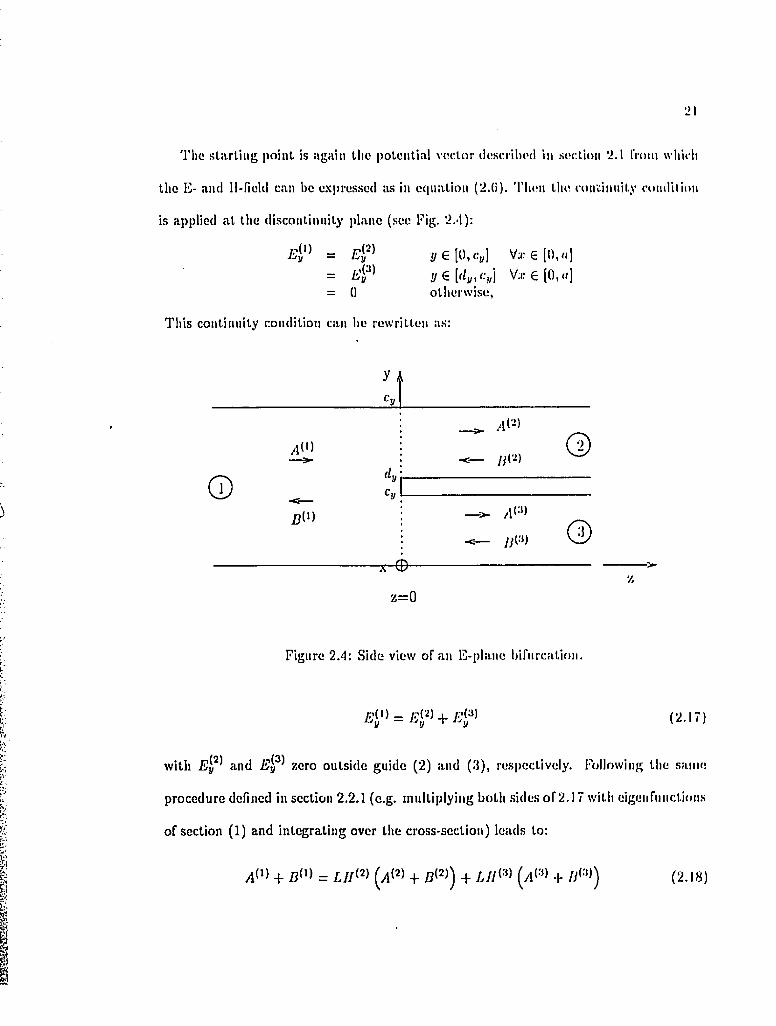
Tlio starling point is again the potential vector described in section 2.1 I’roni which
the E- and H-field can he e.xpresscd as in equation (2.(i). 'I'lnni the continuity condilion
is applied a t the discontinuity plane (see Fig. 2.-1):
I /G[0 , c,;] Va:e[(),n]V:re(0,</]
otherwise,
This continuity condition can he rewritten as:
,1(1)
/j(i)
y A
T - e -
%=0
l id)
/!(:')
■c—
©
©
Figure 2.4: Side view of an E-plane hifnrcation.
/?}') = + 4 ^ ) (•2.17)
with 4 ^ ^ and zero outside guide (2) and (:j), respectively. Following the same
procedure defined in section 2.2.1 (e.g. multiplying both sides o f2 .l7 with eigenfunctions
of section (1) and integrating over the cross-section) leads to:
(2.18)

22
A S(!Con«l and third equation can he found by applying the //jj-fiold matching condition:
//J;’’ = Ilx y € [ 0 , c j V.x-6[0,«]= / / l ^ ^ ! / € ( d j , , C y ] V z € [0 , a j
which yields:
~ _ y jd lJ (2.19)
_ g(3) = ^^(1) _ ( 2 . 2 0 )
Rearranging all three ecpiations leads to the three-port scattering m atrix of the E-plane
discontinuity:
/ üC ) \ / S u S i2 5'i3 \ f \(2 .21 )
/ IJW \ Su S i 2 ^ / A C )
= 5 2 1 5 2 2 5 2 3 / J ( 2 )
1 \ 5 3 1 5 s 2 5 s 3 y Z)(3 )
2.3 Convergence analysis
The convergence behavior depends on the ratio r//p of the num ber of modes taken
into account in each guide. Tlic best convergence behavior is obtained when this ratio is
equal to tlie ratio of the waveguide heights. This is shown in Figure 2.5 and the results
confirm those from [30]. Since tiie step ratio is 2:1, the optim um beiiavior is obtained
for q = 2p. Although the choice of qfp can be different, other ratios will load to slower
convergence.
A similar convergence analysis can be performed with the height as a param eter in
Ka-band (Fig. 2.0) and in VV-band (Fig. 2.7) or with the frequency (Fig. 2.8). These
curves, computed with the same number of modes in both guides, show the convergence
speed decreases with the size of the step and with frequency. Figure 2.9 presents the
convergence analysis for a power divider (the dimension are given in Table 2.1).

•j;5
0.5]) = 'hi
0.48
= 2 1 )
O.'l'l1050 U515 20 10
Niiiiil)t:r o f Moili.’s
Figure 2.5: Convergence aiuilysts of an E-plane step disn)iit.iimil..v iiiid its e(|iiivaleiil. capacitance.
The convergence speed can ho improved by taking advantage of the .structural .sym
m etry of the step, which means considering only even modes with respect to the y-
direclion^.
Only the first 6 or 8 modes are necessary, which is small in comparison with the
calculations done For the same kind of s tructu re by Dittlolf [10]. The m ethod in [H)|
uses two potential vectors, and and reaches convergence oidy with a large
num ber, about fifteen, of T E and T M modes.
^considerhiG odd modes with respect to the x-directioii is not necessary, liecait.se tiie S -m atrix linksc o n s id e n iiR iT E (;)toT E (g .

24
l-Vl-il
lî = 3.848 nim
0.9 2C GHz (Ka-Omid) n = 7.112 iiim, I) = 3.556 mm
0.85
B = 9.288 mm
0,80 15 205 10
Number of Modes
Figure 2.0: Convergence analysis of an E-plane step discontinuity.
B = 1.316 mm
0.9B = 2.540 mm
90 GHz (W-Baiul) a = 2.54 mm, b = 1.27 mm
0.8
0.7 B = 3.356 mm
0.60 5 10 15 20
Number of Modes
Figure 2.7: Convergence analysis of an E-plane step discontinuity.
•Jri
:i = 2 .5 'l m il l
1) = 1 .2 7 m i l l , n = 2 .2 1 m il l
0.9G 5 10 15 20
N m ill ie r o f M o d u s
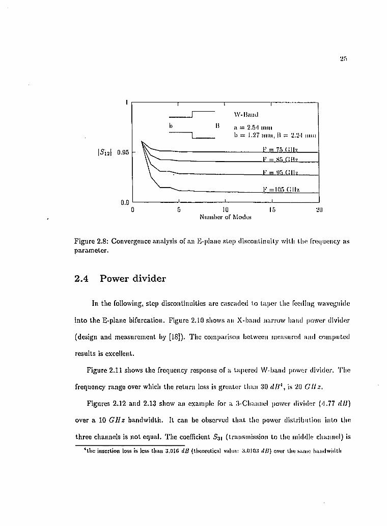
Figure 2.8: Convergence aiuilysis of an F-plane .sl.e[i dlscoiiMmiily wil.li 1.1m freiiimimy :is param eter.
2.4 Power divider
In the following, step discontinuities arc cascaded to taper the feeding waveguide
into the E-plane bifurcation. Figure 2.10 shows an X-liand narrow band power divider
(design and measurement by [18]). Tlie comparison between measured and computed
results is excellent.
Figure 2.11 shows the frequency response of a tapered W-baiid power divider. Tlie
frequency range over which the return loss is greater than 30 (IH‘\ is 20 C I I z .
Figures 2.12 and 2.13 show an example for a 3-Cliannel power divider (d.77 dlJ)
over a 10 G H z bandwidth. It can bo observed th a t the power distribution into the
three channels is not equal. The coefficient .?3 i (transmission to the middle channel) is
^tlic insertion loss is less than 3,DIG dJ3 (theoretical value: .'i.OlO.’S d/J) over ihe sam e liaiidw idth

2G
U.8
0.(5
lO.S
200 5 10 15Number of Mocle.s
Figure 2.9: Convergence analysis for a VV-band power divider (a t 90 G H z ) , fed by a 5-step taper transition (data in Table 2.1)
slightly different from the coefficients S^i and 5'.u (transmission to the upper and lower
channel) which is due to the different power distribution in i/-directioii in the last step
of the taper. The power distribution reaches a peak in the middle, right in front of
channel 2.
2.5 Diplexer-Triplexer
2.5.1 Diplexer
The power divider structure can be combined with filters. Using E-plane metal
insert filters leads to a very compact and easy to fabricate diplexer or triplexer device.
Both filters can be photolithographically etched from a single metallic sheet and then
embedded into the split block housing as shown in Figure 2.14.
The scattering m atrix of the filters contains only modes. However, the power

s [(113]
locl -----
40
30
20
10
10 12 13 M If)Frciliiciic.y [G ll/J
Figure 2.10: Frequency response of nii optimized tnpeied X-l):in<l ]>ower divider.
S [cl 13]
40
30
20
10•S'il = .S’rji < 3.010
80 1000085iTCcpieiicy (G Hz]
Figure 2.11: Frequency response of an optimized tapered W-baiid power divider.

28
: s ü
20Channel 1 Channel 2 Channel 3
828076 78Frequency [GHz]
Figure 2.12: Retiini loss versus frequency for an optimized W -band 3-channel power divider.
S [dll]
d . < )
' 1.8
'1.7Channel I Channel 2 Channel 3
80 82 8476 78Frequency [GHz]
Figure 2.13: Insertion loss versus frequency of the different channels of an optimized VV-Band 3-channel power divider.

2‘)
Figure 2,14: Perspective view of the diple.xer arraiigeineiit with hulder-sliaped metal insert E-plane (iltors.
divider S-matrix connects modes with i constant. If d, and d^, the respective
length in front of each channel (see Table 2.1), are “long enough” , the 7 modes
with Î > 1 and > 0 vanish rapidly and their effects on the filters become alm ost non
existent. Therefore, to interconnect the tapered bifurcation with the filters, only the
part of the S-matrices th a t contains T modes is considered. T hat re<|«ires calculation
of the S-matrix of the tapered bifurcation with dilferent 'I'Effj excitation several times
and to store only the T E f ^ - l o - ' r elements.
The first example is a Ka-band diplexer designed at 28.2 G H z and 82,7 G H z (see
Fig. 2.15). The second example is a VV-band diplexer designed a t 08.5 G H z and 00.0
G I I z (sec Fig. 2.16). The corresponding d a ta is given in Tables 2.1 and 2.2. In the
W -band example, a theoretical return loss better than 20 dH < 0.05 dli ) has been
achieved in both channels. Such good performance could not be obtained with the Ka-

30
band dijdexer because both channels arc closer to the cut-off frequency®. This moans
the dispersion effect is more pronounced and, therefore, the taper is not as good over
the wide frequency range it was designed for.
2.5.2 Double band-pass filter
Combining the output of the diplexer by the same power combiner as the
one at the input leads to a double bandpass filler, which can be useful for different
a])plications. One application may be for high power signals where the power is too
high for a single filter to handle. In this case, the power is split into two channels with
both filters working at the same center frequency. Another application may be to design
an extreme broadband filter where the passband of one filter s ta r ts a t the end of the
other piussband.
A double band-pass filter has been designed with a 2.0 G i l s guard band and more
than 25.0 dI3 rejection between both passbands. The theoretical insertion loss is less
than 0.5 (IB in both passbands (Fig. 2.17).
2.5.3 Triplexer
Expanding the bifurcation to a trifurcation leads to a triplexer for which the
performance is given in Figure 2.18. A good optimized triplexer was difficult to obtain.
One reason is that the power distribution into the different channels is not perfectly
equal. Another reason has to do with the propagation of the first higher order mode
in the last section of the taper. Thus, part of the energy of the fundam ental mode is
transferred into this second mode and it is difficult to control it. T he dimension of this
last section is 2.51 m m x d.Ol m m . Calculating the first three propagation constants
*\VU-28 waveguide: 21.081 G H z

:u
s [(ID)
60
40
20
26 27 28 30 31 33Freqiioticy [Gli'/j
Figure 2.15: Frcciiioiicy rc.spoiise of the optimized K:i-I);tiid diplexer.
80
GO
20
92 93 95 9894 96 97Frc(|ucucy [GIIz]
Figure 2.16: Frequency response of the optimized W-baiid diplexer.

3 2
S [dlî] 30
20
10
92 96 9893 9-1 95 97Frequency [GIIz]
Figure 2.17; Frequency response of au oplim im l double-band filter.
a t 90 (7 //z gives the following values:
TE^o : ;3= 1424 .M m -^
T E n : /? = 1189.29m -'
T E i 2 : /9 = - ; 6 5 3 .4 Q j n - '
Therefore, in the last section of the tapered feeder, the T E \ \ mode can propagate once
excited.
In case of a parallel-connected multiplexer with a number of ou tpu t channels larger
than three, both problems (power distribution and propagation of higher order modes)
are detrimental to good device performance.

80
60
S [dB] 40
20
92 9593 98Frequency [GHz]
Figure 2.18: Frequency response of the optimized VV-band triplexer.

Filter 1 m
Filter 2
Two Channels Three ChannelsPower Divider Diplexer Power Div. Triplexer
X-Band W-Band Ka-Band W-Band W-Band W -Banda 19.05 2.54 7.112 2.540 2.54 2.54
6.75 1.080 8.95 1.95 1.55 2.60Li 6.25 1.125 8.25 1.62 2.19 2.60L3 3.78 1.055 8.55 0.19 1.99 0.36L.i 6.74 1.077 8.45 1.46 1.77 2.10Ls 6.80 1.563 8.30 0.60 2.30 0.17
i h 9.525 1.27 3.556 1.270 1.270 1.270I h 9.74 1.316 3.684 1.309 1.772 1.279I h 10.55 1.489 4.169 1.489 2.340 1.388lU 13.12 1.847 5.216 1.847 2.938 2.436i h 16.12 2.347 6.632 2.347 3.482 3.152i h 19.07 2.64 7.612 2.640 4.010 4.010
d\ 6.05 1.65 1.90(I2 5.95 1.74 1.35(k 1.52
Tabic 2.1: Mechanical dimensions of the X-Band power divider, VV-Batid power divider, Ka-band and W-band filters (all dimensions in millimeters).

a
■'(V A’lV + l *<—
/>A'
Ka-band W-bandFilter # 1 Filter # 2 Filter #1 Filter # 2 Filter # 3
a [mm] 7.112 7.112 2.54 2.54b [mm] 3.556 3.556 1.27 1.27 1.27Jo [GHz] 28.35 32.59 93.77 95.97 94.67N 3 4 4 4 4Si & 5/v+j [mm] 0.525 0.647 0.591 0.586 0.58652 &: S'n [mm] 2.539 3.446 1.829 i.829 1.829S 3 [mm] 4.056 1.980 1.980 1.980Li & L/v [mm] 6.311 4.372 1.555 1.471 1..520^ 2 & [mm] 6.397 4.400 1.557 1.473 1..522
Table 2.2: Mechanical dimensions of the Ka- and W-band metal insert fillers.

3 6
C hapter 3
D ou b le-step d iscontinu ities
'I'liis cliaplcr focuses on the analysis aiul design of a parallel-con ncclcd four-
channol innltiplexcr. In the context of this chapter, some other structures (like iris
liltcrs or waveguide transform er) will be analyzed as well and compared with measured
results available in the literature in order to verify the accuracy of the a]>proach taken.
'J'he disadvantage of the diplcxer/m ultiplexer described in the previous chapter is the
height of the last steps of the taper if the number of channels exceeds three. To reduce
the size of the transition waveguide, the channels are parallel connected in two directions
instead of one (Fig. 3.1). This is possible by utilizing a grid divider fed by a double step
tapered transition to gradually match the transition plane between the feeding channel
(« X b) and the grid divider {N a x Mb). Two new types of discontinuities arc introduced
in this chapter: the double-step discontinuity and the grid divider (Fig, 3.1). Since both
discontinuities require an equivalent analysis, the emphasis on the following procedure
is on the double-stop discontinuity.
Three different approaches to analyze the discontinuity numerically are investigated.
The first approach assumes five field components derived from The second ap
proach considers the general case of six field components derived from a superposition
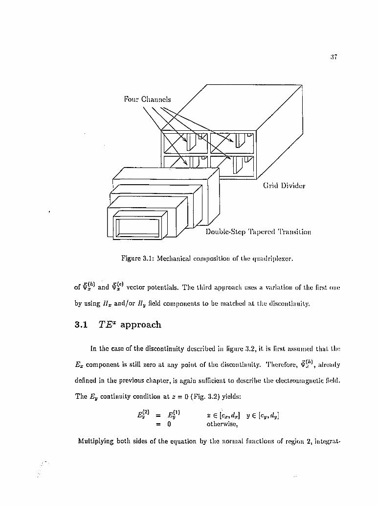
Four Channels
Grid Divider
Doublc-Sl.cp l 'a])ered 'IVansiUon
Figure 3.1: Mechanical composition of the (pmdriplexer.
of and vector potentials. The third ap|iroach uses a variation of the first one
by using 11^ and /or Ily field components to be matched a t the discontinuity.
3.1 TE^ approach
In the case of the discontinuity described in figure 3.2, it is first assumed that the
Ex component is still zero at any point of the discontinuity, 'f'herefore, already
defined in the previous chapter, is again sufficient to describe tlie electromagnetic field.
The Ey continuity condition a t z = 0 (Fig. 3.2) yields:
= E^^^ xÇ.[cx,dx]= 0 otherwise,
Multiplying both sides of the equation by the normal functions of region 2, integral*

3 8
V A
oA i l )
rsU)
AiV
0
% = 0
Figure 3.2: Detail of the double ste|> discontinuity.
itig within the boundaries and finally using the property of mode orthogonality, the
continuity equation becomes:
4 'HD «(DI Jm.nPm.n+ «!,/’ E E a b -yjj" g m V I + W i +
/l(D + /^(2) = f j [ q. (3 .2 )
whore and Jj,„ are the coupling integrals defined by:
r<ixfi.m = / sin( (z - Cr))sin(— z)rZz
Jcx ^
4 . " = ^ '' c o s ( ^ ( y - C j , ) ) c o s { ^ y ) d y
(3.3)
(3.4)
where a x b and A x B arc the cross-section dimensions of the smaller and bigger
waveguide, respectively.
A second equation is necessary to solve the problem mathematically and to ensure
the field continuity for all fields. This equation is obtained by using the //^-continuity

condilion at the d iscontinuity (F ig . 3.2);
The same procedure applied to the E-field leads to the following e(|uations:
- "S?=S Ê i S e g twhich can be written in matrix nolatlon as:
/ l" ) - /j( 'l = /,/i; - //<->) (3.7)
Furthermore, LE^ = LII since:
iM f i& iiS z Ë îi = J -Æ l ZIÜ.ab .2 4 1 ) _ ( ic ) 2 7 .J1) /I B 7 ;(;a)_
If a T E f Q mode excitation is assumed, the matrix L E and LII are the <:oii|)ling matrices
connecting the T E f j modes in guide ( I) to the 'I'Ef,i^,i modes in guide (2). Since two
indices for each mode in matrix notation are not appropriate, new indices Ic/ and /.;//
are defined and their sequences are based on the respective values of the jiropagation
constant. Then the matrices L E and LII are connecting the T/,%' modes to the '/'/,%'^
modes.
Rearranging equations 3.2 and 3.7 yields the S-matrix of the discontinuity. Details
of this procedure are given in Appendix A.
Instead of 7/r, also Jl,j could bo used for the second continuity eipiation (see fig
ure 3.2):
= I l y ^ X e [ C r , < Q y € [ f : , j , d y ] (% -8)

'10
'I'll is <2(iii;il,ioii lüîuis to
' > 1 , ! / - = I , W W ? '»•»>
wiiicli is lincaiiy iiidcpeiulcnt of cqualioas 0.1 and 3.G. It is obvious tha t tlie system
of equations (3.2, 3.7 and 3.9) 1i;ls only two unknowns (namely and /l(^)). This
overdetcnninated system is due to the fact that the hypothesis is not correct: the
component Ex is not zero. However, it has been shown in [28] that, if resonant effects
do not occur within the discontinuity plane, the first higher mode containing an Ex
component is strongly evanescent and its influence on the field matching is small or
negligible. Therefore, it appears to be sufficient to analyze both types of discontinuities
with a five-component field and by neglecting the //y-matching equation.
'I'o evaluate the error made by this approximation, a comparison of this method with
a full wave analysis is presented in the next section.
3.2 Full wave analysis
The full wave approach is bjised on the superposition of two potential vectors
and describing six field components according to:
É = - j c j / i o V X + V X V X ) (3 .1 0 )
/ / = V X V X + jw E oV X (3 .1 1 )
Doth potential vectors individually must satisfy the Helmholtz equation and the
boundary conditions. 'I'he potential vectors arc defined as an infinite sum of normal
modes:
O O C O
'Pi*!.,, = (3.12)m =l M= 0

•Il
= £ E y) -))=U>;=I
where
= 7'1; ;) cos( Av,,x) si n (/.•„,//) (:(•!%)
witli &].. = / 7r /« and = jirfb. '[’lie ])ioi):igal.ioii cotislaiil. is évaluaied as:
l^h ~ - 1 ., - lijij = l:Ô£r - {-^Ÿ - ( ^ y
The expression for the fields derived from has been given already in eipialions
2.6. The fields derived from the eiec.I.ric veelor potenUal tl.f' are given as follows
( ; ; = 0 —► 00, ry = 1 — oo):
4 =) = (// ' - 4 „)T(;;) cos(/:,„;r) Hin(/r„,,yy)
4 ') = si"(/:,,,z) cos(/:„,y)
(:{.16)
= 0
/ /} ') = w E rM /3M C os(t,„z)s in(t , ,y )
7/]'^ = -jw£r,i;;/fcj,„ con{i\.,x)co!i(h,j,^y) 4-
Tp*J denotes the iionnalization factor of the amplitude coefficients which is calculated
from equation 2.7:
T w = . - (:). 17)yaj£/3p,, ( tg fr - ( ^ ) ^ )

42
3.2.1 M atching equation
The clecliomagiietic field is given as an infinite sum of modal vectors. Ai>plying
the continuity conditions at the junction (z = Ü) (see Fig. 3.2):
Z e [ c y . d r ] ! / G [ c y , f / j , ]
= 0 otherwise,
and using the property of mode orthogonality twice:
f E ^ p . { e , x V ^ y l ' f f ) d S = [ (3.18)J a-2 ' Jaj
f Ê^ i^K (c . ,xV ,„ jF j f )dS = f É i } \ { ë , x V ^ y F j f ) d S (3.19)J Al ' JA]
leads to two different coupling equations for the E-field. The second equation (3.19)
which can he rewritten as
yields the coupling equation between modes.
C(2) + £)(2) = i / / (3 ) (3.21)
where is expressed as:
; „(3) _ f . r t 9 -n“ h h ' + ( jv /T ) ) ^ T g ) A B ^
Equation 3.18 is more complex because it includes the coupling between the different
T E ^ modes but also the coupling between T E ^ and T A l^ modes. Rewriting (3.18) as:
•la
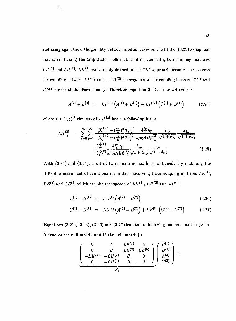
and using again Uic orlliogonality Ijctwucn modes, leaves on I lie Id IS of (a.'i.'l) a diagonal
matrix containing the amplitude coellicients and on the III IS, two coupling matrices
and / , 7 / 0 was already delined in the TfJ-'' approach because it represents
the coupling between TE^' modes. corresponds to the coupling between '/’/v’'*' and
T M ^ modes at the discontinuity. Therefore, ccpiation 3.2d can be written as:
yl(2 ) + j jW = / ,//(!) + /,//<2 ) ^^.(1) ^ (a . 2 l)
where the element of has the following form:
= EE-' + ( § ) ’ T g ' l y i +*«,,< x A T S i J
' C - ! ? ¥ I,., ./j..+ -
r j ' f w/%/ia/3g) v / r + i w y i + /luj
W ith (3 .2 1 ) and (3.24), a set of two ecpiations has been obtained. Ily matching the
H-field, a second set of equations is obtained involving three coupling matrices
and which are the transposed of and
(/1<2) _ / j ( 2 ) ) (:1 .2b )
(.'1.27)
Equations (3.21), (3.24), (3.2(1) and (3.27) lead to the following matrix equation (where
0 denotes the null matrix and f/ the unit matrix) :
/ U 0U 0
0 U LE^^'^U 0
0 0 t/ /
îci
0 \ / /;(') \ / ; ( ! )
a w [
'M
(3.28)
( U 0 0 \ { A(') \0 U C " )
A//C) - U 0
\ 0 0 - y J \ /' ----------------------------- V----------------------------- '
A",
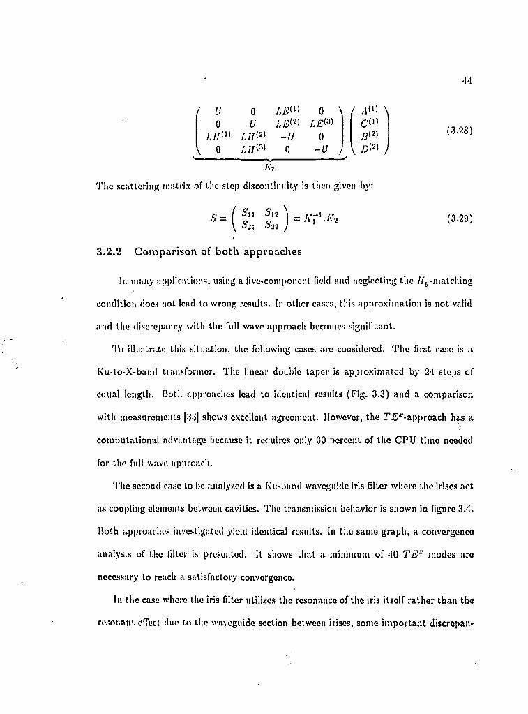
'I’ho sc.atlcriiig matrix of tim slop (iiscontimiily is liioii given by:
. 5 ' = f ç " ç ‘0 = / f f ‘ .A'2 (3.29)\ •■’•il ‘ 'i'i /
3 .2 .2 C om parison o f b o th approaches
In many applications, using a five-component field and neglecting the //y-matcliing
condition does not lead to wrong results. In other cases, this approximation is not valid
and the discrepancy with the full wave approach becomes significant.
'I’o illustrate this situation, the following cases arc considered. The first case is a
Ku-to-X-band transformer. The linear double taper is approximated by 24 steps of
equal length. Both approaches lead to identical results (Fig. 3.3) and a comparison
with measurements [33] shows excellent agreement. However, the Ti?*-approach hé£ a
computational advantage because it requires only 30 percent of the CPU time needed
for the full wave a])proach.
'riie second case to be analyzed is a Ku-band waveguide iris filter where the irises act
iis coupling elements between cavities. The transmission behavior is shown in figure 3.4.
Both approaches investigated yield identical results. In the same graph, a convergence
analysis of the filter is presented. It shows that a minimum of 40 T E ^ modes are
necessary to reach a satisfactory convergence.
In the case where the iris filter utilizes the resonance of the iris itself rather than the
resonant effect due to the waveguide section between irises, some im portant discrepan-

•ir»
l^i.l
O.G
0.4
0.2
1810 12 M 10Frequency [GHz]
Figure 3.3: Magnitude of the reflection coefficient of :i linear Ku-to-X-ljiind traii.sfoniier (approximated by 24 steps), + + + measured [33].
>21
GO
4 0
\ IG m o d e )8 m odes2 0
2 modes
IG12 14 1513Frequency [GHz]
Figure 3.4: Insertion loss of a three-resonator iris-coupled Ku-band waveguide filter, 4 --F+ measured [29].

4 G
dos may occur, in |>arllciilar at frequency close to tlie iris resonance. For example, the
iris shown in figure U.G, Iiîls a cutoff frequency at G7..5 G H z. Exactly a t this frequency,
the 7 7 i^ approach reveals some instabilities due to the lack of the Hy field matching,
'i'he peak at A2.2 G H z corrcsponds-lo the zero of the LE-denominator (equation 3.6)
because the factor which is proportional to:
' A ' X f )becomes infinite at this frequency for i = 2 . 'I'hat explains the large discrepancies with
the full-wave analysis for frequencies within the band [37.5 G H z , 42.2 GHz]. This
discrepancy vanishes when the frequency gets further away from this band. Figure 3.6
is a different view of the performance of the same iris but as a function of the frequency.
Again, the figure shows an important discrepancy around the cutoff frequency (37.5
G H z ) and, wrong results are obtained by using only u T E ^ approach.
3.3 A lternative approach
An interesting solution was proposed in [28]. In this approach, the method
based on five field components alternates between the H^- and 7/y-field matching a t
the discontinuity. The S-matrix is obtained from two coupling matrices L H and L E .
i l l is derived from the Æy-matching equation and its expression can be found using
equation 3.1. The //j.- and 7/y-matching conditions, equations (3.5) and (3.8), lead to
two different coupling matrices LEx and LEy. A now matrix L E is formed by copying
elements from either LE^ or LEy into L E where:
if mode A:, or mode A:;/ is a type= [LEy)^^f.^^ if neither mode k/ nor mode k j i are a type ' ' ' ^

•17
521
iiiin
I = 1.0 mill
3
2
0Ü 2
[mm]
Figure 3.5: Insertion loss of a single resonant iris in a Ka-liand waveguide.
>11
COFull W ave A |)|)ioacli -----
Apjiroacli • • • -
a = 7 . 1 1 2 m i i Il = *{..')•')() mi I c = 'I.OUO m n i d = 1.ÜÜÜ m i I I. = 0.500 m i l l
40
20
3G 40Frequency [GHz]
Figure 3.G: Return loss of a resonant iris in a Ka-band waveguide.

4 8
Therefore, L E œiitaiii.s data wliicli is derived from the matching conditions of eitiicr
llx or Ily. Using the procedure in Appendix A leads to tiie S-matrix of the discontinuity.
This method recpiires the same CPU time as the T E ^ approach and, according to
[28], leads to very satisfactory results in particular in the case of a resonant iris.
3.4 Application to power divider and quadriplexer
'I'he design of an i\-dB power divider can be done by cascading step discontinuities
and a 2x2 grid-divider. 'I'he overall five-port scattering matrix is calculated by using
the generalized scattering matrix technifjues [31]. Fig. 3.7 shows the frequency response
over 10 G I I z bandwidth of an optimized W-band Q-dB power divider. The data for
the power divider is given in Table 3.1. It should be noticed that the lengths of each
transformer section are close to XgfA (at 90 C I l z ) and decrease from 2..58mm in the
first section to 1.92 m m in the last section of the taper. However, the 4 ''- length does
not approximate A,/4 because it is located just between the two biggest steps of the
taper, 3.84 - r 5.18 m v i in x-dircction and 1.81 —• 2.31 m m in y-direction. Therefore,
higher order modes are more excited between both steps and the length L.\ must be
longer to reduce their parasitic effect.
'I'he insertion loss remains virtually constant a t 6.023 <IB^. Furthermore, different
j)|]-responses according to the number of modes arc displayed in the same figure as
well. They indicate that, for example, 30 modes are “almost” sufficient to obtain good
behavior of the return loss coefficient.
The quadriplexer (figure 3.1) is a 6-dB power divider parallel connected to four E-
plano metal insert filters. To match the field a t the power divider output and the filter
'T h e ruliirn loss is g rea ter than 30 dD over the sam e range

•li)
Power divider (all dimensions in millimelers)«I 6 , A„/d a t 90 Cllz
Input waveguide 2.51 1.27 2.209r ' section 2.Ü7 1.33 2.58 2.133
2 '“ section 2.7d l.dS 2.52 2 . 1 0 0
3'"' section 3.50 1.81 2.32 1.895d"' section 3.8-1 2.31 3.10 1.8505*'* section 5.18 2.04 1.92 1.700
Quadriplexer (all dimensions in millimelers)A, di
Input waveguide 2.5d0 1.270 di 1.89section d.921 1.408 1.35 tin 2.07
2 '"' section 5.283 1 . 0 0 1 0.80 d-.i 1.843’"' section 3.001 0.828 1 . 0 0 d,i 1.83
section d.d.35 2.589 2 . 1 0
5"‘ section 5.180 2.040 1 . 1 0
Table 3.1: Mechanical dimensions of llio W-band d-way power divider and (piadriplexor.
5 0 M o d e s , 3 0 M o d e s
3 0 M o d e s \ . 10 M oili . 's V
3 M o d e s
.5 21 = .S'ai = .S’,II = .Sy,| = G.023f//j
1000890F r e r | i i c n c y [ G i l z j
Figure 3.7: Frequency rcs])onse of an oplimixed d-cliannel power divider.

50
iiipiils, the tecliiii<|iie used in section 2 .6 . 1 wiiich consists of .sorting the modes
in order to keep only those which match the filter T E f o modes, is applied.
Fig. . '{.8 illustrates an optimized quadriplexer in the W-band. Note tha t the third
step in the taper is negative creating an inductive effect. This means also that the taper
is not an approximation of a smooth tapered transition.
.Sfdll] dO
92 9593 9694 97 98Frequency [GIIz]
Figure 3.S: Frequency response of an optimized quadriplexer.

M
C hapter 4
C oaxial circular w aveguide
Although atténuation of coaxial lines increa.scs sigiiilicantly with fixnitunicy [:15] and
can reach 2 (IB per foot a t (iO 6 7 / r , coaxial systems are now used up to this fre<pieucy
and arc planned to go Jis high as 100 6 7 / z. For this purpose, lm»( connectors are being
developed. Accurate design of miniaturized coax components is not possible anymore
by considering only the 'I’FM mode, in particular in view of the fact that for fabrication
purposes, some sections of the coaxial device may have large dimensions in which T E n
or even other higher modes can jiropagate. In this chapter, the MMM is a]>plie<l to
analyze discontinuities such as the coaxial inner or outer step (including a change in
supporting dielectric) and abruptly ended rods (see Figure 4.1).
a) Inner step b) O uter step c) A brupt.cnded-rixldiscontinuity discontinuity discontinuity
Figure 4.1: Types of coaxial discontinuities.

52
4.1 Vector potential
Tlio goncnil analysis of coaxial circular waveguide includes T E , T M and T E M
modes. It s tarts from the following equations (equivalent to equations 3.10 and 3.11):
Ë = - V X X V X ( d . l )JWE
/ / = V X X V X ( 4 . 2 )J U / l
where is the T E vector potential and is the 'TM vector potential. The T E M
mode is only a special case of the T M mode. These equations lead to an expression for
the six field components, with E ; = 0 for the T E mode, /T = 0 for the T M mode and
both being zero for the T E M mode. Sec Appendix C for a complete description of the
field com])oncnts.
The following analysis is based on two iussumptions: First, none of liie structures
analyzed in this chapter contains a discontinuity in 0 -directioii and secondly the incident
wave is T E M . Therefore, as shown in Figure 4.2, three field components ( Ep, llg and
E . ) are sufficient to describe the field a t any ]>oints of the discontinuities and, thereby,
only T E M and T M modes arc excited a t the discontinuity.
For the T M mode, in a cylindrical coordinate system, the Helmholtz equation can
be written as:
where k' = to^r-
Using the method of separation of variables, e.g. writing as =
R{p) .^{9) .Z(z) , yields three equations:
^ ^ + k \ Z { z ) = 0 (4.4)

n:
c
Figure 4.2: E-fiolci dccoinposition of au inner stop discontinuity.
d(f
dp
(d.5)
M.G)
with k'i + k'i = Assuming wave propagation in c-direcLioti, cc)iiation 4.4 yields:
Z{z) =
where t . (or /3) is the propagation constant.
Equation (4.6) is a lîcssel diflcrential equation of order n. It is determined hy
considering the boundary conditions. For a coaxial hue, those conditions are (Fig. 4.6):
E- = 0 a t p — a and p = b (4.8)
Since the E~ component is proportional to 9 , the potential vector satisfies also those
conditions and, therefore, the function It. Botit conditions can not he satisfied with a
A (>
Figure '1.3: Side view of a coax cable.
single function like in an empty circular waveguide where (Bessel function of the first
kind) is sufficient. A general form consisting of a sum of independent solutions (J„ and
Af„, Bessel functions of the first and second kind, respectively) is necessary.
/((/;) = IhAhpp) = ANn{kpp) + CJnihpp) (d.9)
The boundary conditions are transformed into:
(4.10)
The propagation constant of the mode is calculated from the root of the
boundary equation. As an example, Figure 4.4 displays the function %(tfo.,„/)) for
different values of vi. All these different functions have a zero at /? = a = 4 m m and at
p = b = 14 mm.

0 .4 :v = 4 . 0 m m
h = 1 4 .0 m m
0.2
2ü 4 8 10 12 14l l î u l i u s [ m m ]
Figmc 4.4: i5c.s.scl fuiicüoii
Finally, since <l>(<il) is g^r-periodlcal, llie following relation mnsl iiohl:
= <!>(/? + 27t) (4.11
In other words, «I> has to he periodic in 0 which reqnires that n he an integer. 'I'lnni
= sin(?i0) or cos(7itf). However, the complete absence of /vÿ and II,, implies that ii
must be zero. Therefore, only 'J'EM and TMo,,,, modes will he jiresent a t the disconti
nuity. Hence, the potential can he rewritten :is:
with two possible and equivalent p-functions:
^Who.,„P) = ~ V " ) (4-1%)

0(5
or
/ ^ t j ( / O = t<ü{kpb).lü[kpi>) - Mkpb)No{kpp) ('l.KJ)
'I’he choice of % will depend on the type of (liscontimiiLy under analysis.
'I'he T E M mode expression is ohtalned by setting kp = 0 (e.g. vi = 0) in etpia-
lion '1.(5. A solution to this ecpiation satisfying the boundary condition exists only if
II = 0. 'I’lierefore:
/^(p) = .4 ln(p) (4 .Id)
The electric field can be written as the sum of modes:
I fiüTüEp =u s p \ /
- J ; E ^>nP,.a\Mi^-,np) (4.15)m = l
where /J(, is the derivative of % defined in equations 4.12 and 4.13. It can been shown,
using integral ]>roporties of Dessel functions [37], that all modes are orthogonal. The
normali/.ation has been obtained by multiplying each mode by o. a is computed by
solving the following Integral;
ft/ Ct Vm (4.1G)
Jtl
where in(p) is the weighting function (m(p) = p in cylindrical coordinates system), the
(.‘„i are the eigenfunctions. 'I'he arbitrary constant Ct is set to 1 . This yields:

4.2 Inner step
For Uic Llicoroticai analysis, an outer stc*i> is exactly e(|nivaient to that of an
inner slo)), llierefore this section deals only with the last one. In the following, a 'I'HM
excitation is assumed generating only 'I'M modes, as it was shown in section 1.1. The
continuity conditions at the junction (at : = 0 ) (Fig. <1.2) yields for the F-Held :
= 0
and for the 11-field
4 ' = € [6 , c]
Separating the 'J'EM and 'I'M modes hy using the property of mode ortliogonalily
defined in the preceding section (including the ninlliplicalion hy the weighting functions)
and integrating within the appropriate hoiindaries, leads to the following e(|uations:
1) for the 'FM mode (e.g. i > 0):
a ' ” + c ' " = (/!!,'’ + « ; ’ ') ( i . i i i i
+ t ("i" + 'f ')9=1 /J; i,- \ l-i - /
2) for the T E M mode:
Equations (d.l9) and (4.20) can be rewritten in matrix form:
/iC) + jÿti) _ i j [ (4.21)

58
Tor tin; //@ in;iU;liiiig coiidiUoii, Uic final ct]iialioii can bo deduced by simply traiis-
posiiijf Uie matrix Ml ( L E = LIE), Tlion using tlie same procedure defined in Appendix
A yields the scattering matrix of tlic discontinuity.
4.3 Results
4.3.1 Convergence analysis
'I'lie first investigation concerns the convergence rate with the radius as parameter
which is shown in Kignre d.5. When the largest outer diameter increases, the number of
modes needed to obtain good convergence behavior increases. Figure d.G illustrates the
return loss as a function of the number of modes with the frc(|ucncy as parameter. The
starting point for all curves is the same because the T E M mode alone is independent of
the frerpieiicy. A large number of modes (for example 15 modes at 50 G I I z ) is necessary
at high frecpiencics to obtain good convergence behavior. This effect is expected be
cause the higher the frecpiency, the more modes can propagate or approach their cutoff
frequency.
4.3 .2 Step discontinuities
One of the first papers dealing with step discontinuities was published by
Somln [d.5] ill I OUT based on research carried out in 19dd ([41J, ['12]). He found that the
erpiivalent capacitance of a step discontinuity can be expressed as:
for the inner step discontinuity and as
C,; =o 4- 1 , ft'*' ^ , do
lOOir— 111-------2 I n + I.I2 10"‘®(0.8- o ) ( r - l.d) (4.23)O O - 0 - 0 + I V /V / V /
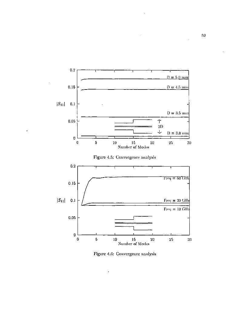
r,!)
0.2
0.15
0.05
1 I 1 ' 1 1 ............ "
n = 5.0 mm
- 11 = 4.5 mm
-
1) = 5.5 mm
- 1 ■■ T - 211
-
1 J , 11 = 5.0 mm1 1 1 t 1
5 10 15 20NimiOi.'r o f M odes
Figure 4.5: CoiivergiMin; atiîily.sis
25 ;» )
0.2
0.15
i ' i . - ( i = : i o G H t
0.05
00 5 10 15 !520 : i o2
N u m b e r o f M odes
F gure 4.0: Convergence analysis

GO
ff)r tlio oiitLT stop (liscoiiliniiity wltli « = (c - 6 )/(c - «), a+ = J + a , « “ = 1 — a and
T — c/a. Soiiilo prosoiilod also a Krajjli for a fiocpioacy corroclion factor. Figure 4.7
compares re.siilts computed from o(|uation (4.2:J) witli tliose based on the MMM. The
figure includes the correction factor wlticli lias been found to be equal to 1 . 0 2 at 1 0 G IIz ,
L5G at 00 G H z and impossible to determine at .50 G H z . As Figure 4.7 demonstrates,
for fre(|iiencies higher than 00 GH z, .Somlo’s approach does not provide accurate results.
a = 4.0 mm " c = 1 2 . 0 mm
200o =
C - Ü
:iOGllz
l O G l I z ^ ^
0 .1 0.2 0 .5 0.8o
Figure 4.7: Coaxial line step capacitance (in f F f c m ) , for a step in the inner conductor. Dolled line from [45] (including the corrective factor).
More recently, other papers have dealt with coaxial discontinuities (Gwarck [43] and
[44]). Gwarek presents the analysis of axially symmetric coiixial discontinuities using
the Finite Difference Time Domain (FDTD) method. A comparison was made only for
the 7 null, 50 ÎÎ, dielectric su])ported AFC7-N adaptor. Figure 4.8 shows the return

(il
loss of such adapter computed with the MMM and the I-'D'l'I). 'I'lie agreement is belter
at low frerpicncies which could be an iiidicntiun that the mesh size in tin; FD'l'l) is loo
coarse at high frerpiencies.
0.Ü4
•S’i l
155 2 0
Figure 4.8: Absolute value of the rellection coellicient versus rrmpnmcy for a line with a dielectrically supported (polysteren) center conductor. Dotted line from [4.'l]
4 .3 .3 Very low-return-Ioss adapter
The design and optimization of a very low return loss taper from V- to K-
cable using the MMM will be shown next. Using an o[)timization routine’ , the stejj
discontinuities have been alternated in order to maintain the impedance as close a.s
possible to the input impedance (50 Q). The <;ptimized adapter is shown in Figure 4.0.
For comparison, an optimized adapter without alternating steps is presented as well.
’ a niulli diiiiciisioitnl searcli iiicthod or iitiivariatc search iiielliod [Glj

section 1 2 3 4 5J.eugtli [mm] 0.2325 0.8350 0.4825 0.6725 0.2575Outer radius [mm] 0.8805 0.8805 1.0301 1.0301 1.1990Inner radius [mm] 0.2540 0.3113 0.3113 0.3057 0.3057Impedance [fî] 57.7 48.3 55.5 48.1 54.9
'I’jihlc 'I.l: Data for an optimized iow-retiirn-ioss adapter.
G2
A l t c r i i a l e d s t e p s
• • • • N o i i - a l l o r n a l e d s l o p s
S.W.IL 1.Î
10 20 30 50 COF r e q u e n c y [ G H z ]
Figure 4.9: SVVR of an optimized V- to K-cable taper. Dimensions in Table 4.1. Maximum SWR: 1.0058 at 15.5 G U z (dotted line: optimized nou-altornated taper)

(1:1
4.3.4 Coaxial filters
Coaxial lilters are imporUml compoiieiils iii coaxial sy.sloiiis, Inw-pass liller
is coin puled, cascading several discouliiiiiilies of iiigli and low impedance seclions ( 1 0 1 )
and 150fî) will: a dieleclric ring to support. I lie strnci nre mechanically. The lillm" was
originally designed on the liasis oFecpiivalenl network theory [:!S). A comparison helween
the measured filter response and the simnlalion with the MMM, using 10 modes, shows
pcriect agreement (see Figures d.IO and I.II).
A 700 i\I II z low-pass filter and a 3 67/c2.J-.sc'cl ioii low-pass filter have heen analysed
as well. The simulated V.S.VV.U response of the first filter has heen compared with [ f.Sj
and the second one with [47]. In holh cases, the good agreement is illusl ralinl in Figures
4.12 and 4.13.
Finally, the last filter to he analyzed is a three-cavity bandpass filter operating
in Ka-band at 37-38 G II : (see Table 4.2 for dimensions). The structure is initially
designed from an equivalent circuit prototype ha.sed on a Tschehyschelf analy.sis and
then optimized taking the effect of higher order modes into account (Fig. 4.14). The
filter shows the following properties: insertion loss in the passhand is less than 0.4
dn , the lower stopband is more than 20 G I I : and an upper guard hand more than 30
G I I z (Fig. 4.15). However, a low frequency passhand (0-1067/.:) can not he siqipressed
for this kind of filler structure since it is a perfect D.C. transmission line. Since this
may cause problems in certain ap])licatioiis, the next section presents a bandpass filter
structure which eliminates this lower ]iasshand.

MMM ----
lü
00.50 1.5 2 2.5 3
Frequency [GIIz]
Figure '1.10: Coin]):u'isoii of a 2 G H z low-pass coaxial filter.
'1
S\'i 2
MMM — Measured Iiy [38] +
+À.0 0.5 I 1.5
Frequency [GHz]
Figure d .11; Kxpauded view of the 2 G H z low-pass coaxial filter.

(if)
•2
V.S.VV.R
1.5
1.21 . 1
1lÜÜ 701)
I'Vciiiiciicy [MHz]
Figure '1.12: Cotuparlsoii of a TOO M Hz low-pass coa.xial lilü'r, -1- + + lueasiirinl
1.Ü8
1 .0 6
V . .S .W .R .
1 .0-1
+ +
1.02
2 :iF rc ip ti . 'iic y [C: Hz]
Figure 4.13: Compari.soii of a 3 G H z low-pass coaxial filler, + + + measured by [47|.

fJG
70
GO
50
S [tIH] 40
00
•JO
10
037 38 39 4035 41
Frequency [GUz]
Figure 4.14: Ka-ba,iul bandpass coax filter.
80
70
GO
S [dU] 50
40
30
r F i l te r H and ( I .O G H z )10
00 10 20 GO30 50 8070
Frequency [GHz]
Figure 4.15: Broad baud view of tlie Ka-baiid bandpass coax filter.

()7
section 1 & 5 2 k. *1 3Resonator Length [mm] •1.30 2 .2-1 4.-10Iris 1 & 0 2 k 5 3 k 4Iris thickness [mm] 0.7G0 0.520 0.352Iris radius [mm] 1.337 1.30S 1.375Outer radius [mm] 1.-K»Rod radius [mm] 0.025Ring permittivity 2.510
Tabic '1.2: Data of llic Ka-tiaiid bandpass coax filler (all dimensions in millimeters).
4.4 Filters w ith gap
Since the coaxial waveguide has an inner conductor, the D.C. current and very low
frequency signals cannot be filtered out by using stejj discontinuities which only alter
the inner and outer diameter. In order to get a true )>assband filter with no such lowpass
property, the implementation of a series of gaps in the center conductor is necessary.
4.4.1 Analysis of the coaxial gap discontinuity
As for the inner (or outer) coaxial step discontinuity, the following assumptions are
made: First, the structure is ^-symmetrical and, secondly, the incident wave is T F A 't .
Tlicrefore, three field components { A',,, IIq and E- ) are sullicient to desciibe the field
a t any points of the discontinuity (Fig. d.Ki) and, thereby, only 'I'M modes are excited
in the empty waveguide.
In the case of an empty circular waveguide of radius b, the boundary conditions are
reduced to /J. = 0 a t p = b. The iiessel fuin of first kind, ./„, satisfies the Helmholtz
equation (d.6 ) and the boundary condition. Thus, It can be rewritten as:
Rif)) = Jnibpff) z (4.24)

Ia
t
Figure'KHk E-Field decomposition nl. a couxial gap discontinuity.
with the boundary condition: = 0. The periodicity of <!>(/?) indicates that n
must he an integer. Furthermore, the complete absence of Eg and lip allows a choice of
n = 0 (only TM^pn modes).
The electric and magnetic fields tangcm,.,il to the discontinuity plane are obtained
as:
I ÇO= - — E (4.25)
" m=l
/ /o = - E « m A n T ,n J '(A : ,„ p ) (4 .2 6 )111=: I
where o,„ is the ortho-normalized factor:
ûffi —v/2
(4.27)PO.in
After the field expressions arc known, it is now jiossible to apply the mode matching

()!)
procedure a l the gap diseoiitiiiuity (at c = 0) (Fig, -I.Hi) :
= 0 p (E [()) a I
and
I I =11(1^^ /> 6 («,/)).
Using again ihe properly of mode orllioguiialily, e.g. eacli conliniiily etpialion mul
tiplied by the weighted orthonormai Cuuctioiis and integrated within the appropriale
boundaries, leads to the following ecpiation (im inding the mode) for the /v,,-lield;
" 1" + " ! " = ,,5 - ) +
v=l Pi • i -1(2 ) ^ /;(2 ) ^ ,11 ^ .jd) ^ „l\)^ (,|.'jb)
where are the coupling integrals:
_ 11 (2 ) 11 . ( 2 ) alc'i^^lh ( 4 ‘ «)-Aj( )■ ' I '< S , (2)U , ( l | 2/i; — li.,1
^’A'.u = / >il){i4^^f>W=Ja
For the IIo matching condition, the final ecpiation is obtained by simply Iranspo.sing the
matrix LI I (LB = L H ‘) yielding:
/ f O - /?(') = LB - /Jf'-'*) (d.UO)
Finally, using the procedure defined in Ap])endix A yields the scattering matrix of the
discontinuity.

70
4.4.2 R esu lts
• Convcrgoiictî analy.sis
TIic first iiivesligalioii concerns tlie convergence rate for the calculation of tlio equiv
alent capacitance of a coaxial guide terminated I)y a circular waveguide (frequency as
parameters). Tlie coax cable is .'J/d inch in radius (Fig. 4.17). A comparison (dotted
line) is given with results from [.52] where the Kayleigli-ilitz variational technique is uti
lized to obtain the etpiivalent capacitance from the coii])litig matrices. In Figure 4.17,
the upper dotted line (at 220.18 f F ) has been calculated at 1 G I I z and the lower one
(at 219.49 J F) at 1 h l l z . Therefore, at low frecpiencies ( \ h l l z and 1 G I I z ) , 20 modes
are sufficient to calculate the capacitance, whereas 0 0 modes are necessary at higher
frequencies.
Tabic 1 . 0 compares results from different methods tised to analyze this type of dis
continuity. Results from the MMM have been obtained using 24 modes which are
sufficient to achieve a 0 . 1 % accuracy.
Radius FretiResult
from [52]Result
from [45]Result
from [40]Result
from [49]This
Method7 mm 1 kHz
I GHz80.00 79.70 79.7 79.88 79.0380.70 79.7 79.917 79.67
14 mm 1 kHz 1 GHz
104.50 159.40 159.4 159.70 159.27104.85 100.039 159.53
3/4 in. I kHz 1 GHz
219.49 210.89 217.0 217.40 216.50220.18 217.7 218.07 217.17
Tabic 4.3: Values { f F) for the discontinuity capacitance of a 50 0-coaxial guide terminated in a circular waveguide. [52]: Rayleigh-Ritz variational technique, [45]: Approximation of the eigenfunctions using llahn series, [40]: Interpolation of Somlo s da ta , [49]: Least-square boundary residual method.

c [ n - ]
2 '1()
2:iü
21Ü
20010 ‘10
N iim l)i;r o f Mtuit;;
Figure 4.17: Convergence analy.sis for Uie e(|nivaleiil capacitance of a coaxial guide terminated by a circular waveguide for different frecpiencies, dotted line calculalanl from [52], upper line at 1 G i l s (220.IS f F ) and lower line at I (*210.4!) f F ) .

72
• Sliort-üiidcMi coaxia l caUlu
A sliorl-eiidcd coaxial caldt; is also analyzed and coiii])aied wllli results from (ijô,
j)|). 178-179). At low rre(|iieiicies, a perfect malcli lielweeti both methods is observed
(Fig d.18). However, since tlie forimila used in is independent of the frerpiencies,
the discrepancy incre:ises with freipiency.
C [pF]
-I
:i
2
1.0 GIIz
0 . 1 0.30.2Length [mm]
Figure 1.18: Equivalent capacitance of a short-ended coaxial guido.-|-F+ computed by [:i5l
• Gapped coaxial fillers
On the basis of the previous analysis a gapped coaxial filter has been analyzed.
The structure uses half wavelength resonator sections separated by quarlei wavelength
coupling section ([38], pp. d77-'lSi). Each coupling section works as K-inverter^. A 21
*\Vliich is .111 iiupcdnncc triinsfoniicr, from %» a t one end to Zi, = l \ ^ j Z a a t the o ther end.

7a
G H z bati(lj)!uss filter in a (K 118 Willron) semi-rigid ceaxial eahU? has been designed and
optimized {sec Tai>Ie d. 1 for the dimensions). A qnalilalive corrected electrical length
Outer Radius [mm] 1 .2 U.bInner Radius [mm] 0.041A/2 Sect. 1 k 7 [mm] 4.252 (0.0Hi)A/4 Sect. 2 & 0 [mm] 1.400 (3.104)A/ 2 Sect. 3 k 5 [mm] 4.290 (0.000)A/4 Sect. 4 [mm] 1.51() (3.274)Gap 1 k 8 [mm] 0 . 0 2 0
Gap 2 k 7 [mm] 0.072Gap 3 k Ü [mm] 0.031Gap 4 k 5 [mm] 0 . 1 1 0
Tabic 4.4: Data for the o])timized gajijied a-section coaxial tiller, corrected electrical lengths in parentheses.
(dctined in [38], pp. 479) h:is been added in the Table 4.4 in order to obtain a better
simulation of the K-invertcr circuit. The corrective value has been estimated to 1.794
m m (a t 2 0 GIIz) . Figures 4,19 and 4.20 shows the response of the optimized lilt.er.
The next passhand is a t 39 G I I z which allows a sto])baii<l of 18 GHz between the two
passbands (Fig. 4.20). This stopband may be improved i)y cascading a, 30 G I I z lowpass
filter (structure defined in section 4.3.4).

7*1
S [.I H]
r » u
20
10
2 G18 222 0F rc iU ic n c y [G H z]
Figure *1.19: S-parameters of a gapped coaxial fdtcr.
M O
120
1 0 0
2 5 3 0 3 55 10 15 20 *10F re q u e n c y [G H z ]
Figure 1.20: Broad baud view of the gapped coaxial bandpass filter insertion loss.

C hapter 5
M etal-insert circular w aveguide filter
The circular waveguide is an imporlaiil Iraiisinissioii iiiediniii lor aiileiiiia feeding
systems due to i l s direct compatihilily wil.li the üehLs in horn aiilcniiins and because two
orthogonal polarized waves can propagate simultaneously inside the giiiile. Moreover,
the circular guide has the advantages over the rectangular waveguide of greater power-
handling capacity and lower attenuation for a given ciitolf wavelength.
In analogy with the inctahiusert lilter in rectangular waveguide [‘J 2 ], in this chapter,
a metal septum loaded circular waveguide handpass lilter is presented and analyzed
(Fig. 5.1).
The qiiasi-rcctangular discontinuity of the metal insert is appro.ximatanl hy a how-tie
shaped discontinuity (Fig. .5.2) to avoid dealing with W-dependent boundary conditions.
This is computationally more efficient since the residting eigenfunctions are mathemati
cally easier to handle. This kind of discontinnity has not been treated in the literature'
before and provides the basis for the ficid-theory designs of iiiettd insert filters in circular
waveguides.
’ the eicctrom agnelic field in lliu sector waveguide li:i,s Ijeeii only skeiclied in [.’>0]

7(i
Figure 5.1: Structure of tlie iiictal insert loaded circular waveguide filter.
V ' .
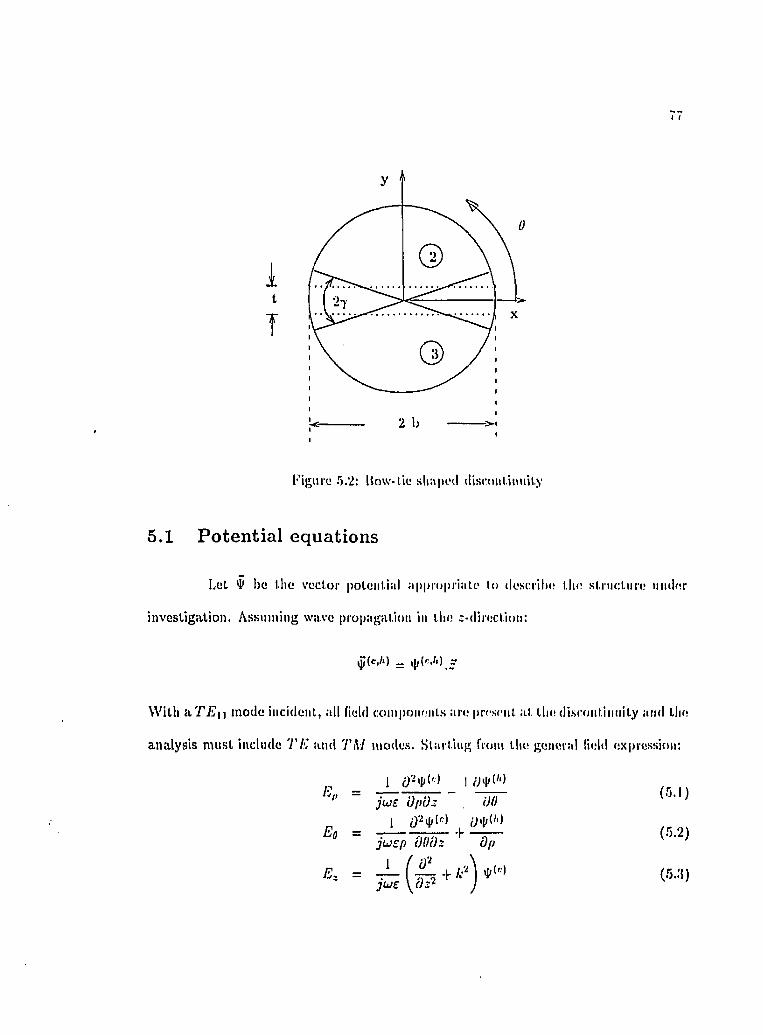
1t
T
Kigui'o 5.2: Uow-lie slin|iml disniitlimiil.y
5.1 Potential equations
L o i $ 1)0 I h o v o c l o r p o lo i i l i a l J i p p i o p r i a t o lo d o s c r ih o l l io s l r i i c t n r o ii i idor
i n v e s t i g a t i o n . A s s u m i n g w a v e p r o i i a g a t io i i in l l io z - d i io c l in n :
W i t h a T E \ i m o d e i n c i d o n l , a l l field coiiijioiioiiL.s a r e prcscn l. al. t h e d isco i i l . i i i t i i ty a n d t h e
a n a l y s i s m u s t i n c l u d e 77 C a t u l T M in o d e s . S l a i t i n g f i o m t h e g e n e r a l field e x p r e s s io n :
1 I ( ) ¥ > ' )
ju>£ O p O z 00
E q =1 o ¥ ' ‘
+j u £ p OOOz dp
(S. I)
(5.2)
(5.:!)

78
T E or T M modes c;ui be obtained by lotting = U for T M mode fields and = 0
for T E mode fields. The electromagnetic field in each subregion of the filter is a linear
superposition of both 'TE and T M fields. The Helmholtz equation:
..
(with = fv'ijfr) is solved by using the method of separation of variables, e.g. one can
write the potential as:
l l {p)M&yA-) (5.8)
This yields three independent equations^:
5.1.1 0-equation
The first refers to the fAecpiation and can bo written as follows:
A solution for is:
<l>l''*i(tf) = Asm {k l ‘' '^k) + iJcos(4 "''‘>f )
where the constants A and B are determined by applying the boundary conditions:
^Oiily two equations will be discussed since the :-cqualion lias the obvious solution Z { : ) =

a l 0 = 7
a l = Â — 7/•/,, = = 0 and 11(1 = 0
Allliougli llio liouadary condilion are tnily sliglilly diliereal l'ur '/’A/ and 'l'IJ iiuides,
they lead in f a d In Iwo very dilierenl snlulinns.
1) Tor the TM inodes, according lo e<|iialion 5.:(, /A = *1' ' * and is pro-
porlional lo ’riierefore llie fMioiindary condilioa in llie upper guide (seclion
(2), Fig. 5.2) can lie rewrillen as:
,4 sin(/.g^7 ) - f / / cos(/,- '*7 ) = I)
.4sln(A{''^(- - 7 )) + /icos(/.'^'‘*(- - 7 )) = 0
for which ihe solnlion is;
(|'(')(W) = .sill (/.•'■ ’( « - 7 ))
with = v i t / ( 7T - 2 7 ). For the lower guide (seclion (.'}), Fig. 5.2), llie .solution i.s:
«Ill'll(f ) = sin - 7 — 7r)j
2) In the case of T E modes, Ep = and 'I'^'l a 'l»*'‘)(W). The hoinidary
condilion becomes:
fcg‘^4 co.s(iy*S ) - /4^‘*yJsin(/:y*^7) = 0 \co.s(A:J ‘’(:r - 7 )) - B sin(/4^‘*(tt - 7 )) = 0 J \ l:H' = ftn
yielding
4>f ‘ (fl) = cos(&y^(0 - 7 )j in ilic upper guide
^('^^(0 ) = cos — 7 - 7t)^ in ihe lower guide
In the following, i> =

80
5.1.2 ^;-equation
'I’lit! .secdiid C()uaUoii is tin; />-(;(|ii:il,ioii:
wlierc jj, iippor or lower waveguide, by imposing the
boundary conditions, the solution is a sum of Ijessel functions of both the first and
second kinds. However, Hessel functions of the second kind have an infinite value at
j) = 0 which is physically impossible for this structure (Fig. 5.2. Therefore:
The potential function in the upper guide (an etpiivalcnt ex])ression is obtained in the
lower guide) is expressed as:
with
= kh r -
5.2 Field expressions
'riio taiigenlial electric field can be writLcii a.s follows:
y C O C O
^ Y , (5.10)n=a m = l
C O C O
- E E ' d ; ? ( t v . , + ^ , . , ) s ïp=0<)=l

fSl
Tlio suiicrscript (c) liulicalos 'I'M modos and tlio siiporscripl (/;) 77v modes. Tlie
parameter f is eipial In 0 in tlie case of a circular empty waveguide and I iu the case
of a half circular waveguide, lo lake into account the fact that the Tii/u.,,, mode does
not exist in the latter one. Furthermore, the eigeufunctions c satisfy the orthogonality
property, i.e.:
= (5.11)
The delinitioii of the vectors e,J,m and are given in appendix D as well as the
I IT'-norinalization factor 7',^li and j for each siihnigion of the lilter.
In the empty circular waveguide, any wave can be decomposed into two orthogonal
waves. One t vpe o'" mode is marked with the superscri|it “s” and denotes the mode with
the E-field perpendicular to the septum. The second one is marked with the superscript
“c” and denotes the modes with the E-field parallel to the septum. However, the 7'A/»,„
modes exist only as "c"-modes and the 'I'lCu,, only as “s”-modes.
The tangential magnetic field is written as:
H r = E Z ’ S . i ' ' ”- - " ” - ) '" ! ; ! . .r.= j rii = l
' p=0 7= I
The definition of /imj,, and //{vj are given as well in Appendix I).

XU
5.3 M atching equations
In order to obtain the S-Matrix of the li-jiort discont.iiuiity, the tangential electric
held is matched at the discontinnity, e.g. ; = 0 (Fig. 5.U);
• 4 P = 4 " ^ ] ,= É P 0 6 [tt + 7 , 23f - 7] > V/J e [0,/;] (5 .1 U )
= 0 0 € [0 , 7 ] i [ ^ “ 7 i ’î‘ + 7 ] and (Uzr - 7 , 2 »] j
where the different fields E-f are defined in ecjnation 5.10. Since the tangential electric
field in the empty circular waveguide is expressed as the sum of four indepcmdent and
orthogonal sets of eigenfunctions, \ ' o ' ! j i ’(*sp(n:l.ively, the mode
matching procedure is made possible by successively multiplying ecpiation (5.12) by each
eigenfunction and then integrating over the circular waveguide cross-section.
5.3,1 First coupling equation
The first coupling equation, e.g. equation (5 . 1 2 ) multiplied by r i- j '’’* and iiil,egra.ted
over S\ leads to:
[ 0 ) d 5 = f É^^Kclj'''^wif)JI]dS -\- f /z-'-yP.c -j '"^ ) r / . S 'JS\ ' JS2 ' •'Sn '
By introducing the expressions for the clifierent /■>/■, Lliis equalian cun l)e rewritten ns:
. r 1 0 3 CO 1 CO O j
JSl I Wtl <*^-1 „ = = l
= X f ~ E E 4 S ' r £ > -
JS2 L ^ ^ 2 p=Oq=t- r 4 00 00 00 00
+ £ - i - E E ^ m ? ' - E E 4 f ' 4 f“'*3 (. ‘*'‘ 3 „_1 ,)=Ü7=I
p d p t l O
(.5 . 1 :5)
f / d p d O

S3
wlien;
+ /ill;:») (5.m )
/ & = (/il',:' + ) (5.15)
+ /;();)) (5.1G)
4 !;" ' = 'C '':) ( c y + / ; y ) (5.17)
4 n i' = / & i u J (Aiiil + (5.18)
4 f ’ = + (5.19)
Similar relaUoii.s arc obtained for the lower guide (suporscript (3) instead of (2 )). The
LliS of e(|iia.tioii (5.13) is simplified by using the orthogonality property of the eigen
functions, i.e. ecpiation (5.11):
and
* OD C O
-1- E E C ' S ( / i s . + m.) I IH=l 1)1 = 1 ^
+ Ê Ê r , ! 7 ' ( c + D ® ) r f (5 .2 0 )
I C O O D f t
+-r E E « ï » ("& + "S. / . I11=1 T,1=1 ' Jir+TT JO
+ Ê E ' r ' “ > ( c s + f l)3 ) r " ’ t e ' 4 ! j " y x «p = 0 , = l ' '0
Finally, the coefiicients >1 -^* and have been isolated on the LHS of (5.20) and
are a function of all eigeu modes in the upper or lower half guide. The next step is the
calculation of the coupling integrals:

SI
1 ' Coupling integral
The first, coupling inlcgral concspoiuls lo llu; coiipliiig liulweou llie 'I'M modes in llie
upper half guide and ihe T M ’* modes in the drciihir waveguide. With /i : 1 — co and
Î : 1 —♦ oo:
—1 flic j ; = r ~ ' I '
J-y */U
This coupling inlegral is zero if ii — i is odd. 1 or n - i even:
2'" Coupling inlegral
This coupling inlegral corresponds lo Ihe coupling helween ihe 77v modes in llie tijiper
half guide and Lhc 7’M* m odes in ihe circular waveguide. Willi p : 0 — co and
i : 1 oo:
c i i =J~f Jo
This coupling integral is zero if p — i is odd. For p - i even:
C l i =
The third and fourth coupling integrals are com puled from the coupling integrals
C l f and C'/g. The p-coupling integrals do not change, contrary lo the //-integrals which
are modified when u - i is even and n * / odd. In this case, the sign of the integral is
inverted.

8 5
E()ii:iU üii 5.20 can now be rewritten in terms of matrices:
/ i " ' ) + + (5.21)
In the case of 7 = 0 (infinitely thin .septum), the matrix equations can be simplified
since the respective coupling integrals are ctpial to zero = 0 and = 0 ).
Eurtliennore, the remaining matrices are diagonal and their (/:, t)'^^ element can be
evaluated as:
, 7 '(c’.2) /% rp{e3) rr
where the k corresponds to the order of the propagation constants of the T M i j or T E i j
modes arrangc<l in decreasing order, respectively. IJoth elements equal \ / 2 / 2 in the case
= £-2 and £| = S3 . The infinitely thin septum looks like a perfect power divider for
this kind of mode. Therefore the output power on each channel is exactly 1/2.
5.3.2 Rem aining coupling equations
The solutions for the second, third and fourth coupling equations are given in detail In
Appendix D. Only the principal results are given liere.
The three remaining coupling equations are:
f 4 ” .c / j ' ‘ ’ii;(/>,<;)r/5 = / / Ép.e}^^ ' '^w{p ,e)dSJS^ j5 j ' JSj '
f = / l3p .e l ' ^ ' "^w{p ,0 )dS+ / Ë^^KêPl^^^w{p,e)dSJSi J S 2
f = I £5?>.c/j“">îe(/î,t )d.Ç+ f Ë ^ ^ K ê i f ‘^w{p,Ô)dSJS\ J $2 Js^
Using the same procedure as in the previous section leads to three matrix equation
.S(i
(from Eqns. D.l, D.4 iuul I).5):
E : -I- /.//*'-'■' I /;'■-’) H- (r,.2'2)
H : + / ; < ’•’> = (C'(-) + / ; ( ' ) ) + / , / / ( ' ' '") I- /;(:')) (r).2;j)
H : + £)<'■-'> = A//(''2c) ( c ' ( ' ) + /;•*•) + +/.//<'"'"> -i- /;*•'>) (r).2.|)
The matrices ;,|,d ;ne zc>iu (see Appendix I)).
5.4 Scattering M atrix of the discontinuity
Four matrix ecpiatious liave boeii ohtaiiKs! 5.21, .3.22, .3.2:} and .3.24, one for each
type of polarization: 7'7i’, 7’/?'"', T M ’’ and 'I'M'', respectively. A .similar derivation can
be made for the ll-ficld. It can be shown that the ll-Iield conpliiiK matrices are the
transposed of the equivalent. E-field coupling matrices, e.g. = LII^'''^' for any
superscript X .
/l{2) _ ^(2) = A/.X':'") (/iC-’) - /zC’)) + ( / l ' ’’-' - / / “ ">)
C'{ ) _ j){i) = (/id -’) - A f i ( C ’d ’) - / ; “ •■')) ..p
+ z,z-;i'' ") - zzd- i)
/l(3) _ ;j(3) = Z.Zid3-’) ^y^dd _ Z,Z-jI'-'d (y ldd - ZZd'd^
- zp( i = Az;("'') ( / id 'I - z /d ')) 4- z.A'd"''') (c'd-’i - z ;d ’) q.
^ y.(Mc) ((^'(14 _ y;d^)j q . (/id--) _ /yd'^l)
This set of equations is reduced in order to simplify the analysis and the program
complexity. This reduction is acliiovcd by summarizing all waves propagating in the
same direction in one vector ( Fig. 5.3):

87
I -------- ^ e w
-------- >-: < -------- fi'i)
-<--------
/.’{I): -------- ^ E(:))
: < --------
/<=0
Figure 5.3: Structure of the (li.scuutimiity
1, lu the empty circular waveguide
&(') = and =
If each vector is of size (A'l x 1), then and will be a (4/V] x 1) vector.
/ /jC 'l \niic) p[U)
2. In the half circular waveguide (.1=2 or .1=3)
If each vector Is a (A^j x I) vector, then and will be a { 2Nj x 1) vector.
For a rectangular waveguide discontinuity^ it lias been shown in [31] tha t certain ratios
of the different modes A'j have to be satisfied to obtain fast convergence. For the
bifurcated circular waveguide it is assumed that these ratios can be expressed as:
A^2 = A 3
ill p .itltcular tlic Infiirc.iteii waveguide

S8
TIiosc ra.lios give sciuare mat rices uiui the (utiplinK <‘<|iia!i(nis can be rewrit ten as:
/ J / b MI)
\ 0 /j/b*-’*') y
( A//(":=") /.//("•'•’) \AZ/b-’ '-') A/Zb'i'-I
0 /.//(A I,)V 0 A//b"'‘-> /
= A A //l-l(/ ;b -l + /'('-l) + AA//b'l(Z:'b')+/.'b^^^
4- fC:)) 4- (5.25)
(5.2(i)
(5.27)
The AA//b^i matrices arc of .size (-lA'i x 2A'j).
f A ü b ^ l U M^ AA'b-') A/ib*'-) AA'b'-')
= aa / ';< -i(a’C) _
£ ( 3 ) _ / . - ’(3) ^ A A / v b ' ) ^ /e ( t) _
(5.2!))
(5.:!0)
The procedure to obtain A A is ecpiivalejit to tlial, of AA/v'-). 'I'lie A A A' matrices
arc of size (2 A 2 x dA'i ). From e(p:ations (5.27), (5.:(0) and (5.50), the scattering matrix
of the discontintiity can be derived;
1( S n ■S' , 2 Si:i
= S 21 S-12 •5*231I % i S:\2 S'33
/ ( ( + / ) - ' ( ( - / ) 2 (^ + / ) - ‘ AA//b^> 2 ( ^ + / ) - ‘AA//b’) A A g M ( / - .S 'n ) / - AA/vb^),SVj -AA/tb^lS',;,
\ L L F J m - Si I ) - A A/vb'O.v,., / .. AAA'b').Yu(
with ^ = AA//(^)AAA'(^) + AA//b'0/,/,/i(3) ;,nd I the identity matrix.
To illitslrate the method, the field distribution h;is been computed from the scat
tering matrix assuming a T E i , mode incident wave parallel to the septum. Figures 5.d

Sü
jiiui 5,5 si low tlio rcsulLs with Jiii septum migle of 4.0 ami iO.O <lc’g. respectively. 'J'he
imniber of modes is 50 in both cases {e.g. IS 77'’*, IS T K ‘ , IS Ti\I'^ and IS T M ‘ in
the circular waveguide and 50 77i and 50 T M in both part of bifiirrated waveguide).
5.5 Convergence analysis
A convergence analysis of a 1mm long .septum shows tha t a minimum of 40
77‘f and 7 7 / iiio<les are necessary for acceptable convergence behavior (h’ig. 5.0). For
a longer se)>tuni, the convergence is reached with fewer modes since the interaction of
modes in the bifurcated waveguide is less .significant because they are more attenuated.
As stated in section 2.5, the convergence behavior depends on the ratio of the number
of modes taken into account in each guide. A convergence analysis of a single bow-tie
shaped discontinuity is shown in Figure 5.7. Ilelatively fast convergence is obtained
with the ratio 2A'i = A'%. A certain instability can be noticed when the ratio is too low
(e.g. a small number of modes in each sub-guide).
For small angles (less than 10 degrees), the coupling between T E and T M modes is
negligible (Fig. 5.8 and 5.9). Therefore, if an incident T E mode is assumed, the analysis
can be carried out with only T E modes. This assumption is not valid for angles greater
than 7 c which hucreases with the frecpieucy. For frecptencies above the TA'/oi mode
cut-off frecpiency, the omission of the T M modes in the analysis leads to wrong results
(Fig. 5.9).
5.6 Bandpass filters
The filler structure is composed of a series of resonant cavities separated by
coupling septa. The initial filter was synthesized with lumped clement theory [57].

}) ( )
Figure 5.-1: i î l c c l r i c field d i s l r i b n l i o i i w il l i <i \ in c id e n t , w n v e p u r n l l e l l o Die s e p L im i ,
7 = -1 d e g r e e s .

Ü1
Figure 5.5: Electric (ieki distributiou witli a T E \ \ incident wave parallel to the septum, 7 = 1 9 degrees.

i)2
5 | , [(iB]
1) = 4.00 mi l l L = 1.00 H i m V = 31.00(311%8
I. tlnK..G
4
2
00 10 30 40 50 GO20
NimiOer of Modus
Figure 5.6: Convergence' analysis for a melal .sepliim loaded circular waveguide
I'reil = 31 G11% Angle = 2. Beg. I) = 4.0 mm.10
9
80 10 20 40 50 GO 7030
N u m b e r o f M odes {A'j )
Figure 5.7: Convergence analysis for a metal septum loaded circular waveguide with di fièrent mode ratio as parameter.

D.3
S'h [‘1»]
All triodes O nly TI3 m o d es
31 G H z
3
2
00 3010 40 45
A ngle [Dog.]
Figure 5.8; “Slue” iiolarizcd wave iii.scrtioii loss versus tlio angle of a sejrtum loaded circular waveguide ( “Siiic” polarized wu’."; defined in section 5.2).
All m odes----Only TE modes • • • -39 GHz
0 10 30 40 45Angle [Deg.]
Figure 5.9: “Cosine” polarized wave insertion loss versus the angle of a septum loaded circular waveguide (“Cosine” polarized wave defined in section 5.2). The peak on the 39 GHz curve corresponds to the upper limit of the 7'£oi mode propagation in the furcated waveguide. *

!)1
Tlicsc lumped elemeiUs utilize K-invertors which consist of :i 'I'-iietwork ami two
transmission lines with electrical length </j/ 2 connected on both sides of the T-net work.
A single T-network corresponds lo a single metal insert and the values of the inductances
may bo obtained by using charts such as the one given in Figure .1. U). From these element
[pJI]
10
30 GHz
34 GHz
32 GHz
30 GHz5
32 G H z2 8 G H z
2 8 G H z
00 1 2 3
L [ m m ]
Figure 5.10: Equivalent inductances of a.sini]>le metal insert.
values, s-parameters are calculated from which the corresponding insert dimensions can
be derived. However, since the higher order mode interaction between subsequent metal
septa is not included in the lumped element synthesis, the initial filter response is off
95
l)y 1 GIJz, Nevüillioloss, tlicsc insert (iiiiionsioiis arc used ;is starting values for the full
wave analysis, and the generalized s-ni-'.lrix of the entire filter is optimized using the
optimization procedure in [22].
Figure .5.11 shows the theoretical and measured performance of a threc-rosonator
Ka-hand lilter in a d m m radius circular waveguide. The measured insertion loss is loss
than 1.0 (UJ in the passhand (0,08 dli computed) while the respective return loss is
greater than 12 dli (18 dB computed). The reflection coefficient for the polarization
per]>endicular to the .septum is greater than 00 d B (85 dB computed) over the operating
range (28 to 88 6 7 / z).
A 81-82 G i f z live-section bandpass filter in a d m m radius circular waveguide has
hecn designed using the same procedure. The theoretical and measured performance is
shown in Figure 5.12. The measured insertion loss is less than 1.2 d B in the passhand
(0.05 d B computed) while the respective return loss is greater than 20 d B (14 dB
computed).
For both fillers, the comparison between theoritical analysis and measurement shows
an excellent agreement. However, the small discrepancy between both curves is due
to the a pproximation of the rectangular septum by a. bow-tie shaped discontinuity, the
losses which are not taken into account in the analysis and the inaccuracy of fabrication.
5.7 Coaxial bow-tie shaped discontinuity
The same filter realization applied in the last chapter, can be used for coaxial
liller.s.
The quasi-rectangular insert is also here approximated by a bow-tie shaped discon-

!Ki
S [dB] 20
30 3228Frf;([iiciicy [OIIz]
Figure 5.11: Performance versus free;ueiicy of a 3-iesoiiat.or circular waveguide filter,
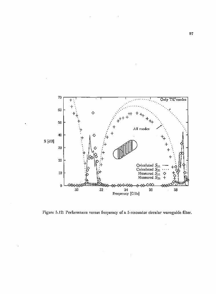
97
S [(II)]
70
00
50
dO
;io
20
10
+ +++++
Only T E m odes
Ail modes
++ ■.
++ •.
C a lc u la te d 5 n ----- , ^C a lc u la te d 6 2 1 - - ^
Mcîusured O " t Y M easured .S ';, + ^ '
O'IFrcciiicucy [G II %]
30
0
Figure 5.12: FciToniuiiiee versius frequency of a 5-resoiiator circular waveguide filter.

!)S
nRadius[mm]
k[GHz]
Septum length mm] Uesonator length [mm]T| = T»+, Ti = 7 ;. f a ~ / II—1 L\ — L,i A'J — 1 A;i
3 4.000 29.22 0.844 2.985 5.0.83 5.7085 4.000 31.08 1.079 3.991 1.012 4.0.87 4.702 4.701
Tabic 5.1: MccliHincal dimensions of (lie K:i-I>:uui lliree- and five-iesonal.ui' circular waveguide filLor.
tinuity (figure 5.1%). The expression for (die eleclromagiiel.ic field in terms of normal
modes and the analysis of the discontinuity follows the same steps as in the circular
waveguide. Starting with the general field definition, eipial.ioii (5 .1 ) . .(5.0), the 1C- and
li-fields are expressed as functions of the pol.ential which must satisfy the Helmholtz
equation (5.7). Considering that the 0-boundary condition in the coax and in a circular
waveguide are identical, the solutions of the 0-differential ecpiation are:
In the coaxial waveguide
In the upper half waveguide
In the lower half waveguide
__ J sin(»0) cos(?/0) ./ m II integer
<l>*'*(0) = sin(i/(0 - 7)) <1>* '*(0) = cos(f/(0 - 7 ))
<l)('-)(/y) = sin(</(0 - 7 - 7r))
‘1>* '*(0) = cos(;/(0 - 7 - 7t))
with u = titt/ (7T - 2 7 ).

99
1t
î
Figure 5.13: Mêla! insert discontinuity in n coax waveguide and its approximation by a bow-tie si)aped discontinuity

t o o
The soliiUoii of the /J-dHIorontial cqii:ilioii (5.9) is a sum of two Itessel fimciioiis.
Tiiis is the only ])ossil)ilil,y lo sulisfy Uie l)oiiii(l:iry comlilioii (-l.S):
U{lcp) = A'y(/vii)./„(/i7 )) - ./„(/i/;)A'„(Av>) 'I'M Modes
Il{kp) = i\'Ulcb).}„(kp) - Jl(l:h)i\\.{kp) TIC Modes
with u = VKf{iT — 2 7 ) ill the iijiper or lower half waveguide and 1/ = ii in the coaxial
waveguide.
In comparison to the empty circular waveguide, the coaxial waveguide supports a
T Ë M mode as well. 'I'lie expre.s.sioii for the 'I'KM wave is ^.^-independent and its R.-
function has already been described in eipiatioii (d.l I).
The expression for the tangential 1C-Held is the following:
. + /; (5.:u)n = s Tri=.i 00 00
;i=0 ii=\
where e denotes the orthogonal eigenfunctions. Thêir expre.s.sioii can be found in
Appendix E. The parameter s is equal to (I in the case of a coax wa veguide and I in the
case of a half coaxial waveguide to take in account the fact that the 7'A/o,„, mode does
not exist in the latter one and lo include I he 'I'EM mode (corres]iouding to the
mode).
Again the superscripts “s” and “c” in the coaxial waveguide describe the polarization
of the E-fiald.
The tangential magnetic field is written as:
; 'T = E E ' 2 , (/I.....n=5 î«=51

1()1
J OO QO+ — E Z D ' J P t ' i c ' „ - « , , , ) % !
/ ,)=Ü7=1
Tli(! (icfinlUon of /tmî„ and are given in Appendix B.
In order U; obtain the S-Matrix of the :i-port discoiitinnity, tiie tangential electric
field is matched at the discontinuity, e.g. z = 0 ( Fig. .5.13):
&/' 0 E [if,7r - -y]= A'y e [tT + 7 , 27T - 7 ]= (I f''G [0,7], [--7,?r + 7] and [27r-7 ,27rj ,
^pe[ ( i ,b ] (.5.32)
where the different A'y fields are defined in equation (5.31).
Following the same procedure defined in section 5.3 leads to the LE and LI I matrices
from which the threeqiort scattering matrix of the discontinuity can he derived.
The presence of the TEM mode makes a slight difference in the procedure which is
presented here:
The first coiqding equation is obtained by multiplying equation 5.32 by the T E M
orthogonal function cjg** and by integrating over .5‘i:
f / Ë V4l'hü[p,0)dS + f É?\4!o\o{p,e)dSJS\ JSj JSs ’
Using the orthogonal property of the eigenfunctions yields:
n = \ 7ri = l
+ z f : % : ) ( c ' K i + DKi) ’ ( 5 .3 3 )r=Oq=l •'T “'0
+ E E + ASi) / I pdpde11=1111=1 */0
+11 fin'.? ( 4 3 + 0f3) / r ’ V' We11=0,1=1 JO

I ou
The cocfTicioiits and have hoeii expiessed as a fiinelioii of (lie sum of all
eigenmodos in the upper or lower half guides. 'I’lio nexi st ep Is (o calculate the coupling
integrals:
Coupling integral
The first coupling integral corresponds lo the coujiliug helween the 'I'M modes in (he
upper half guide and the TKM modes in the coaxial waveguide. With n : I — co:
Chn = r ~ "J n
This coupling integral is zero if n is even. Ibr n odd:
Clot =
2’“ Coupling integral
This coupling integral corresponds to the coupling between the 77v' modes in (he upper
half guide and the TEM modes in the coaxial waveguide. With p : 0 — oo:
C'lo2 = f [J'y J a
this coupling integral is zero if p is even. For p odd:
rb j
c%2 = Ja pp
The third and fourth coupling integrals are computed from the integrals Chw and CUn.
The /j-coupling integrals do not change, contrary to the tf-integrals which are modilied
when 71 — Î is even and n * i odd. In this case, the sign of the integral is inverted.
5.8 Bandpass filter
The filter structure is composed of a series of resonant cavities separated by
coupling septa. Following the same procedure presented for the circular waveguide
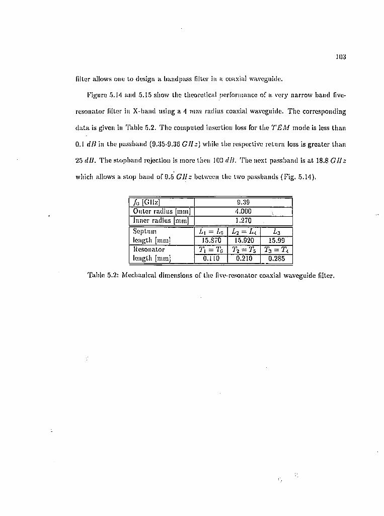
io:3
(illcr allows one to design a bandpjuss filter in a coaxial waveguide.
Figure 5.1 d and .5.15 show the theoretical performance of a very narrow band five-
resonator filter in X-baiid using a d rinii radius coaxial waveguide. The corresponding
d a ta is given in Table 5.2. The computed insertion loss for the T E M mode is less than
0.1 f//i in the ]>assband (0.35-0.36 GHz ) while the respective return loss is greater than
25 ( in. The stopband rejection is more then 100 dll. The next passhand is a t 18.8 G H z
which allows a stop band of 0.5 G H z between the two passbands (Fig. 5.14).
/o [GHz] 0.30Outer radius [mm] 4.000Inner radius [mm] 1.270Septum length [mm]
Ij\ = !j5 Ij2 = TL.t 7»315.870 15.020 15.99
Hesonator length [mm]
r , = 7c 72 = 7s 73 = 71,0.110 0.210 0.285
Table 5.2: Mechanical dimensions of the five-re.sonator coaxial waveguide filter.

MU
250
200
100
50
00 2 10 12 Hi kS() 8
i’Vi.’(|ui;n<:y [ G i b
Figure 5.14: PciTorm:utco ve< :us fiXMiiienc.y of a 5-re.soiiali)r coaxial incl al-in.sorl. waveguide filler.
140
120
100
S [dB]
9 9 .1 9 . 2 9.:S 9 .4 9 .5 9 , 0 9 .7 9 . 8 9 . 9 10l 'ie q u c iic y [G il/.]
Figure 5.15: Expanded view of llie .5-iosoiialor coaxial iiielal-iii.serl waveguide filler.

1 0 5
C hapter 6
C onclusion
'i'lie major ulijoclive of liiis lliesi.s lias lieen lo develop an accurate mimcrical
melliod to analyze and design fillers and mnlliplexers for niillimeter waves, in particular
in a circular waveguide. 'I'his cliapter completes lliis work by giving a conclusion and
recommendation based on tlie experiences gained during tins thesis. As well, suggestions
are made regarding further work in this area of ; ésearch.
6.1 Results
The major objective of this thesis has been to develop an efficient method for the
analysis and design of waveguide filters and multiplexers at millimeter waves frequen
cies. The MMM apjilied to different kinds of discontinuities iias sliown its capability lo
analyze these different devices accurately witiiout the aid of supercomputers. Further
more, the analysis of most of the structures lias l)een made by matching only two field
components instead of four.
For example, in the parallel-connected dipiexer configuration introduced in Chapter
I, tiie vector potential was sufficient to describe the electromagnetic field in the
vicinity of an F-piane discontinuity, and only the matching of two field components {Ey

!(1()
and //j.) is required, 'riiorefore llie numerical iirucedure resnliinn from itiis analysis is
CPU time ellieiu'd and accurate.
The «[uadriplexer, introduced in (lha))ler d, is an extension of the dipiexer con
cept. Discontinuities involved in this (piadriplexer require four fndd components to he
matched. Chapter 3 has shown that, when there is no resonance at the discontinuity,
the matching of two field components is suliicient to «lescrihe tite discontinuity.
After characterizing selected discontinuities in rectangular waveguides, this thesis
h:is focussed on coaxial transmission lim!s and transitions. The M.MM has heen applied
to different kind of discontinuities, and results have heen compared with tin; litera
ture. Different bandpass filters have heen designed, one using only steps in the inner
conductor, the other one using gaps in the center conductors.
Chapter 5 introduced a circular waveguide metal-insert filter hased on tiie metal-
insert filter idea in rectangular waveguide. The metal insert has heen approximated hy
a bow-tie shaped metal sheet instead of a rectangular sheet. Chapter 5 has shown that
this approximation does not introduce a noliceahie error in the m<;asnr(.'d frequency
response. It was shown that ;us long as the operating frequency remains below the
cut-off frequency of the TMoi mode, a 'I’D mode approach is suliicient to analyze the
discontinuity.
6.2 Further work
Most of the dual or multiple modes filters use a couple of resonant cavities separated
by one or several irises, 'riiese irises provide the coupling between modes and allow the
design of compact filters with very high Q-factor. The values of these coupling factors

107
arc* obtuiiiod by iippruxitiiniioii, iind tlicruforc luniiig sc.icws aio necessary lo coinpciisale
for llie lack of design accuracy [bS]. Tlie reclangiilar irises used for the coupling in [59]
and [no] {dolled lines In Kig. 0.1) could be rejilaced by semi-circular irises (solid lines
in I'ig. 0.1). In lliis case, llie field analysis used in Cliapler 5 can be applied and very
accurate coupling factors can be calculated. Willi respect lo fabrication, this sonii-
circnlar shape of the irises should not introduce any problems if etching tcchni(|iies arc
used. However, in terms of accnrale design (dual mode liIters arc very sensitive to the
posilion and exact shape of the iris) the advantage is obvious.
Figure 0.1: Circular waveguide iris used in multi-mode cavity filter.
The rectangular coaxial filter sliown in Figure 0.2 could be an extension of the work
presented in Chapter2. The analysis of such a filter should include both T E and TM
modes and the TEM mode as well.
The grid-dividcr discontinuity presented briefly in Chapter 2 could be another possi-

IDS
MclulU/4tion
a) From rectangular waveguide tu coaxial rectangular waveguide
b) Step In Inner cuiiduclnr In c) K>plane nielalll/.atlon Ina coaxial rcctangulur waveguide . a euaxlal reaclauguUr waveguide
Figure 6.2; Mctal-iu.scrt coaxiiil recliingiilur waveguide filler.
bio direction for further work by c;uscadiiig it severul times in order to obtain a, squared
waveguide filter for both polarization: an equivalence to the nietal-iusert filter but in
two directions (Fig. 6.3.aj. Following the same idea, but using a. circular waveguide, a.
dual-polarization circular waveguide filter could be analyzed and designed ( Fig. 6.3.b).

109
yy
7
Figure (5.3: i)iial']>olariza.l.ioii luotal-liiserL filler a) in rectangular waveguide b) in circular waveguide.

A p p en d ix A
From th e coupling m atrices to th e scattering m atrix
This appendix describes iiow to obtain the S-inat rice.s IVuiii the coupling ecpiatioiis
which arc:
and
/j(i) = A/j (/1(2)_
The aim is to obtain tlie following two-port S-matrix :
( tfCI \ _ ( S n S u \ ( , | l ' l \I - t , . s v i ) nm j
The first step is to isolate
= / l O - fÆ ( i / z . / i c ) -f -f /,6'.
Then
{Ij -b LE.LIl)B '> = Ua - + 2LE.lf '>

I l l
where l,i rc])re.sciiLs tlio ideiil.il.y matrix. Tlierarore, the expression of .S‘n and S \ i are:
.S':I = + ( / j - AA'./,//) (A. l )
.SVi = A E ./ , / / ) - ' (A.2)
I'Yom the second coupling e(|uation :
= A//..d<’> +
= A/Z./lC) + A//. (.5'ii..d'‘> +
= A//.(A/ + .S'il).d(') + (A//.,S'|.j - A,)
Tlterefore, .S'21 and S 2 2 are ex;)ressed in terms of AAA, ,S'n and .S'lj:
.S'21 = A / / ( A / + .S'il) ' (A.3)
.S'u2 . = A//..S'i-i - A/ (A.4)

W'l
A p p en d ix B
F ield com ponents in coaxial w aveguides
• T M field
dp
0
TE field
Ep —
Eg =
E , =
I
p do
dp
0
Ep ~1
E’- =
En
Eg
/ / z
jbjc Opdz 1
■jucp OOUz
‘ n / ' ,jwf
1 Ü-'l'C')
JW/i dpdz1

li:j
A p p en d ix C
Field expressions in circular w aveguides
C .l Em pty circular waveguide
The eigeiifiiiictioii.s rclalcti to tlic B-field in the empty circular waveguide are:
TM inode (at z=0) :
sin(in9) 1 _ n f cos(nff)j?(c) _ fyO:)cos(iiO) I dp
'I'E mode (at z=0) :
i l
(C .l)
cos(7;éf) I dJp(kj,pl,p) s\\\{])d) j dp (C.2)p [ - cos(pg)
111 this waveguide, any modes can be decomposed into two orthogonal modes. The first
type of mode is assigned the superscript “.s” and denotes the mode with the E-field
perpendicular to the septum. The second one is marked with the superscript “c” and
denotes the modes with the E-field parallel to the septum. However, the 'I'Mom mode
exists only in V ’-mode. On the other hand, the TEu,, mode exists only in “s”-modc.
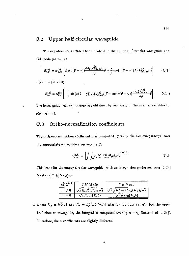
II-
c .2 Upper half circular waveguide
The eigenfiiiiclious lelaLed to the K-field in the upper haif drciilar waveguide are:
TM inode (at z=0) :
f (c) _ ^ (c)71,HI '**71,HI
TE mode (at %=0 ) :
p,<i I'.'i - - si a ( 1 /( 0 - 'y))J,>(lc\!:L(i)f> - cos(f/(f; - 7 )) (C. l )p ................... ■ (Ip
The lower guide field expressions are oiitained iiy replacing ail the angular varialites liy
t ' ( 0 - 7 - 7 r ) .
C.3 Ortho-normalization coefficients
The ortho-normalization coefficient a is computed by using the foliowiiig integral over
the appropriate waveguide cross-section .S':
= j I/, IC .r ,)
This leads for the empty circular waveguide (with an integration performed over [0,27r]
for 9 and [0, b] for p) to;
T M Mode T E Mode
71 7 0 v/5F/i'c./;,(A'c)/\/271 = 0 , / ^K J x U < ,b ] v/%A'/,7(j( A'/,/;)
where A'/i = lipn,inb and A'c = lipn,mb (valid also for the next table). Tor the upper
half circular waveguide, the integral is computed over (7 , T - 7 ] (instead of [0,2%]).
Therefore, the a coefficients are slightly different.

l lô
I 'M Mode T E Mode
71. ^ 0 y ; r - 2 7 A W : ( A c ) / 271 = 0 Does not exist i/tf — 2 7 A;,./u( A/i )/v^2
These results «lo not change when coiisUleriiig the upper lialf guide or the lower half
guide.
C.4 M agnetic field
Tlie elgenfuiictinns related to the inagiietic field in the eiiijjty circular waveguide arc:
TM mode (at /,=()} :
71 f cos(7)fi') \ f sin(?wP) \/>•) = o(')*‘ n , m /7 1 -.sia{?76‘] I ' ” 1 cos(utf) dp■i)
T E mode (at z={j) :
f sin(ptf) ] dJpUclilip) p f cos(pg) I / fi.(à)1 codpO) f f * 1 -^d u ( ; /n( cos(pfl) J dp
and in the upper half guide:
TM mode (at /,=()} :
r,(c) ="■n,m “ ii.ra
T E mode (at z=Q) :
'>K = - « sin(/4tl - 'i cos(;/(tf -
C.5 Norm alization coefficient
This cocllicieut is oi)tained by computing the following integral:
X /7*).d:sj = E,J10 - E o I!;)z .d S ^

1 11)
F o r a n y t y p e o f g u i d e , e .g . c in jJ ty , u p p e r l ia l f o r lo w e r lie If w u v e g u l d e , s o l v in g th i s
i n t e g r a l l e a d s to :
' j f X = l'"i- Hie 'I’M m o d e s ((.Mi)
a n d
ï ï ï , = , / - ^ C ' - nPn.jij

117
A p p en d ix D
C oupling integrals
D .l Second coupling equation
'i'lto .second coupling c<|uation is (.lie inatcliing etinnlion (5.12) iiiultiplicd by and
iiit.ogralcd over (lie empty guide section:
/ [ Ê p\(rÿ'''^w(f,J](lS+ f Ép.êff‘'- w{p,0)dSJSi J S2 J S3
Expressing tlie tangential fields and
is, V ' > (cl-i) _ _ !_ V ' n = l 7/1 = 1 M=OtM = in=U 7/1 = 1
C O C O
- Z Z C " e " - E E 4 !; ' ' ’4 ‘"’;>=ü)/=] ;)=Ur/=l
pdpdQ
~ L
" 1
- I ; ! - ] [ : 2 ,;j=0 (/=]Fi = l n ) = t
L ÿ ' V ' _ Y " Y ' yM/cJ) (/.3)Z— i ""I ‘■<1111 Z j ■‘m t» i/ ) = O i ; = l11=1 1(1=1
.ë-j^^^pdpdd
.c if^ ‘^pdpdO
wlicre /i’miV’', and have been defined in section 5.3.1 as well as BmnK
E'mfJ and However, by using the orthonornial property on the LHS of the

1 I S
équation, it is possible to write:
t ^ y V /•?--> W*A T: ^ ^ i . i ' >\ . . f ' O \ / /
2 „ „ i
+ Z E ■").?’ C + «1,;’ / fy=Oq=l •'''
+ ; : r ê ê ( „ s „ + h ,™ ) f ' " ’
OC» oo #2 JT—n flf+ E E ' " f f ' c ; 3 + / / e ’- ' t " ’," ' ," " '
j,=0.;=I
The equation can be rewritten in term of matrices:
+ / j ( i - ' ) = / ,y / ( c i= ) ( /iC -’ l + /if* ’ ) ) + ( c 'C - i + / ; ( ' ) ) -I-
l j l U : i c ] ^ ^ -I- /;<•■’>) ( D . l )
1'' Coupling integral
The first coupling integral is, for n : I — co ami i : 0 — co:
c / f = I ’" " ' 4 ] ' “' ixtixloJ y JO
= a ( f , ! „ S f > / " ’ s i n ( . ( « - l ) ) c o s ( ; 9 ) , W p,,,. .
/ cos(/y(<?-7))siu(/7;)fW I'/(j P
The ^-coupling integrals are expressed in .^]>penclix hi. 'I'lie coupling integral C’/f is 0 if
n — i is even. For n — i odd:
2" Coupling integral
This coupling integral corresponds to the coupling between the TJi! modes in the iijjper

11!J
liîiir g\ii<l<! :ii»l lli(! iiuxltis ill Liiii drciitiir wavcgiiidu. Willi ;j ; 0 — co and
J : 0 -» oo:
c ; = r ' ' tJ-f JO
= siii()>(f/--/))cos(tfJ)dtf j f ^ ^ (Ip +
- 7))siii(/Y;)fW^ J ' ' ' ^ - f d i ÿ f p y i p
As sliowii previously, Uic W-inlognils are eipial lu zero if p - i even. In Uio p — i odd
case, llie iiilej^ral liecoiiies;
e n =
Tlie tliird and foiirlli coupling integrals are computed from the coupling integrals
C I^ and C'/.j. The p-coupling integrals do not change, contrary to the 0-onos which are
computed over [tt + 7,27t - 7 ]. Their values are siiiijdy niuitipliod by - 1 if i - 71 is odd
with V even (e.g. / odd).
D.2 Third coupling equation
After multiplying with the T/i'" orthogonal fnnction of the T/i' mode, the E-field match
ing eipiatiuii becomes:
JSi JS2 '
. r I CO <x> I CO CO
•'■S'l L * 1 1 = 1 m = l , : = ü m = I
;)=Ui/=l ,:=U ,;= IpdpdO

1-21)
“ i1 co co
Z_, Z j >i'>i ""I Z j Zv i»i^ ,1=1 m = l
1
I
cù <Xi
fullKlO
^ Z j Z-, »i"i ""I Z-i Z^ )"j i"i,1=1 „1=1 ;i=0 7 = l
where Emn^\ and have heeii delincd in e(|iialions (,'5. l l-T). ! <)) as well
as Em ft\ and E p ,f \ Applying ihe orUiogonalily property of modes, l his
equation can he written as:
'4 '! '” ( C + 'Xy') =
Ë Ê ft'3-'S (/<S„ + r^ Ti=l m = l ' *'
OO CO
+ z z ' C ' ( c + " S ) / Ip=ü,/=i •’'<
I CO o o —1
— E E ( / i w , + h ï ;>, / /‘ ‘ 3 „ = ! m = l
CO /•■ J ir- 'i rl>
+E E ''S" (cs + »EI) / , I 4!;" ' - , "W«
+
p = 0 ,(= l
In terms of matrices:
C'(") + JOC') = /.//<'''■’) -I- /,//<''-■’• 4- (D.-2)
1"' Coupling integral
The first coupling integral is (it : 1 — oo and / ; Ü — oo):
r n — f rb
; C IS = J7 VO
= -aKajfi J ' " ' %.(,/(» -

12J
'I'lio arc again c<)iial to zero if ti — i is odd. 'Die n - / even case can be written
as :
c - =
= - < i !< » £ ' * ' I ^ 'ii>
wliicdi means that C/-] = 0, V /, j , n and ui.
2“' Coupling integra!
'I'lie second coupling integral is {with p : 0 — oo and / : 0 — oo):
CI:l = f I cffK eff-''^p(Iptll)J-l JO
= ^ s i u ( i / ( « - T ) ) s i i i ( f f l ) < ( s ^ % / ' ) / ' I
' " S " - -n i
Three cases must be distinguished:
a) p - i odd:
cm = Ü
b)p - / even and //* + P 0:
c ' . ; =

[22
c)p = i = 0
CIS = - 2 1 ) j '
L ik e Cl^t t h e tl ilrcl c o u p l i n g i n t c g r n l is z e r o . ' I ' l ie r ou r t l i c o u p l i n g i u l e g r a i c a n In;
c o m p u t e d f r o m t h e c o u p l i n g i n t e g r a l C ' / ; , . ' I’l ie / ^ - co up l i n g i n t e g r a l s d o not. c l i a n g e , l ike
t h e ^ ' i n t e g r a l s , b e c a u s e fo r i = n, t h e ff/2 coe l l i c i e i i t d o e s n o t v a r y i f c n n i p u l e d o v e r
[7 , 7r - 7 ] o r [7r + 7 , 27r - 7 ]. T l i c " m a t r i x e t p i a t i o u (L<in. 1).;J) c a n , t l i e r e f o r e , h e s impl i l i ( ; d
= Ü a n d L = 0 ):
c ( " ) + + / ; < - ! ) + / , / / ( ' " " ) -I- ( D.-l )
D.3 Fourth coupling equation
T h e f o u r t h c o u p l i n g e q u a t i o n is t h e m a t c h i n g e q u a t i o n ( 5 . 1 2 ) m u l t i | ) l : e d by a n d
i n t e g r a t e d o v e r t l i o e m p t y g u i d e s e c t i o n :
JSi JS-2 ' JSj
B y i n c l u d i n g t l i e p r o p e r t y o f t h e o r t h o n o r n i a l e i g e n f u n c t i o n s in t h e L H S o f t h e e t p i a t i o n ,
i t is p o s s i b l e t o w r i t e :
r g ‘»i (ciy> + =
^ Ê Ê « ' « ,> (/1 5 . + » a ) r r71=1 771 = 1 I ^
+ E E « > (c,S + «S) / Ip=Or/=l '
r ' i i r —'7 r\)
E E C hS ('IR. + «a) / /
+E Ê (C IS + '«) f r i",7=0 7,= 1

)2:î
' l ’Ito « (j i ta t in ii ca ji b c w r iU c j i a ls o iii l e r i i i s o f ii iaLricos:
+ /;('•-') = A//!'''"! (/i!-) +
] Coii[)liiig inlogral
iî.g. 71 : 1 — ' 0 0 and / : 0 — 0 0
./-y J()
~ "i'im « ; J ' J “( !'{(>- 7 ) ) C(M( i 0 )(I0 y_ j^hXc)
œ s(7/(Ü - ' ) ] ) a \ u ( i ÿ ) ( l O ■ " ■ (//)
The /’/-iiil.cgrals arc c{[ii:il lo zero if 77 - î Is cvcii. Iii llio 11 ~ i odd case, the integra!
becomes:
T h i s m e a n s t h a ï t h e coii[) l ii ig i n t e g r a l C'A; = 0 , V i , i , 77 a n d 777.
2 ' “ C o u p l i n g i n t e g r a l
E .g . ( ; 7 : 0 — c c a n d 7 : 1 — 00)
f x — I rb
C/4 =
= - f ' M - 7 ) ) œ s { 76 ) 7/6 ^ ^ ■ J i‘U ^ lS ^ } ,p ) M k ] ! l j^ p ) p d p
r " \ o s ( , / ( 6 - ? ) ) s i n ( 7 6 ) , / 6J o d p d p

I’J-I
It is evident that this integral is zero if [ji - i) is even. In the opposite case ( ( / j - i)
odd), the integral is written as:
: /: p i ■ ,-.J ■ ■ (Ip (Ip
From those results, the matrix cunpling e<|nntiun heroines:
fUlp
C'(ic) + /j(ic) = /,//('>2v) ^^.(2) / , / / ( ' . IV) ( n.5)

125
A p p en d ix E
Full w ave expressions in coaxial w aveguides
E .l Coaxial circular waveguide
Tlie fiigunfiiiictions related to the E-Iield in the coaxial waveguide arc similar to
those of the empty circular waveguide, equations (C.l ) and (C.2). The difference conics
from the /^-function which are:
The 'i'EM eigenfunction can he written, at %=ü, as:
cj,u =
.A.gain, any modes can he decomposed into the sum of two orthogonal modes: the first
type (superscript "s” ) with the E-field perjieudicular to the septum and the second one
(superscript ” c” ) witli the E-field parallel to the septum.

12(»
E.2 Upper sectorial coaxial waveguide
The eigcnfuuctioLis rehilcd to the IC-field in tlie iip[)er semi-sector waveguide are similar
to those of the upper half circular waveguide, e(|uations (C.il) and (Cet). The dill'erence
comes from the p-fiinction which are, in this case,:
The lower guide field ex])iessions are obtained l>y replacing all the angular variables by
1/(0 — 7 — 7T).
E.3 Norm alization coefficients
The a ortho-normalization coefficient is computed by using the integral defined in
equation (0 .5 ) over the appropriate waveguide cru.ss-secl.ioii .S', yielding similar expres
sions as those to the circular waveguide. },,„[>)■, îuid
replacing )&/;), iind re
spectively in the expression of the ortho-normalization coellicients is the only difference
between the T E and TM modes. For the 'I'lCM mode, equation (0 .5) leads to:
“ u,o -
The expression for the 1 VVatt-normalization coefficient does not change when con
sidering a circular waveguide or a coaxial waveguide. Therefore, they can be found by
equations (C.G) and (C.7).
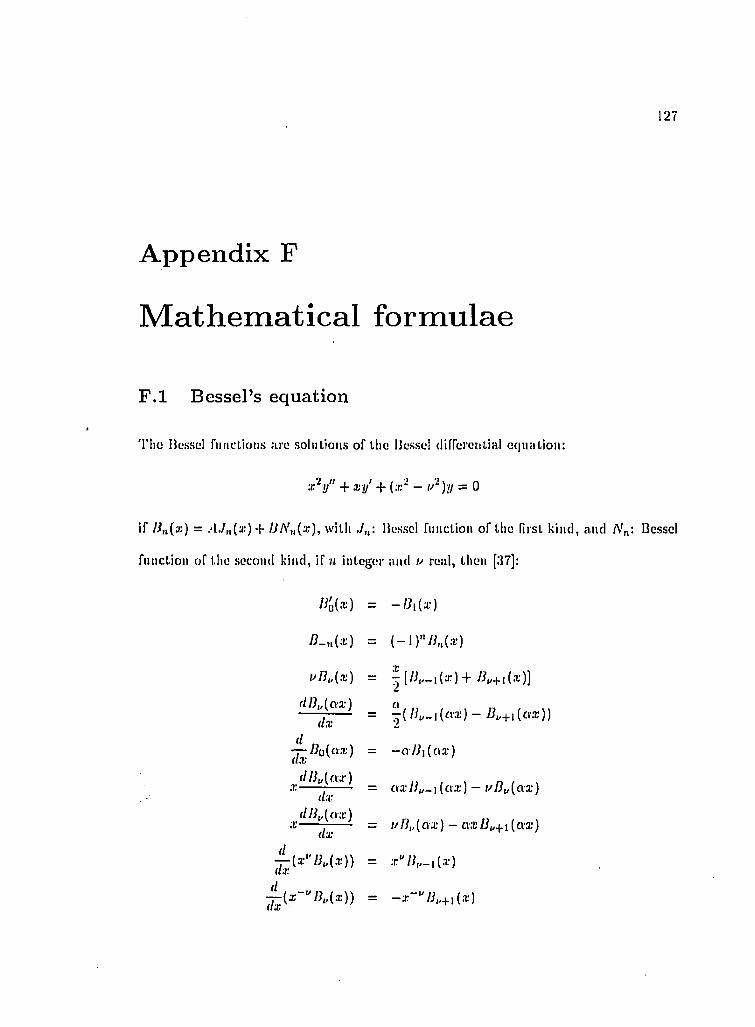
127
A p p en d ix F
M athem atical form ulae
F .l B essel’s equation
'riie Hesse:! fimclioiis ;uo solutions of tlie Hessei difroretiLial equation:
x^y" + a;;i/ + - <^ )y = 0
if = .-l./„(x)+ IJN„{x), with liessol riiiictioii of the first kind, and A»: Bessel
function of the second kind, if n integer and real, then [37]:
yj_n(;r) = ( - i ) ' ‘yy,.(.r)
( / [x] - ^ 1 ( .T) + 1 ( , r )]
= | ( /y,._i (a.ï) - liu+i (oæ))
~ /?o ( ) = — o /y 1 ( era; )
■r— = a x J i^^ i(a x ) — ul3i,{ttx)
(I ( O'tlT );c — ^ ■ = ;/ n,, ( o ;f ) - a x a a ; )
~i . v^' l }^(x) ) = a : " /y „ _ , ( .T )

Integrals involving llessel’s fiiuctioii:
J x^lJü{x)dx - l ii(x ) + xliü (x) - J |}^){x)(i.r
J J3i{x)dx =
J xIJi[x)dx = + J lh ( '<i')dx
j x*'J7y_i(x)f/a; = x^l}„(x)
J x n „ ( a x ) I U f t x ) < l x = z fP ~ (P/ f i l i „{ ( i x) l i „- ] ( f i x) - (\ n „ ^ \ ( n x ) l J „ ( l i x ) \V o - fP )( fi l j„(<xx)U„^i(l ' ix) ~ ( n ; t : ) / / y ( / J , r ) ' \
- ffTTTp j. 2 2 '2
j x B l{a x )d x = + ^ ( 1 -
= ~ [BfA(rx] - //,._!(n;i;)W,,.|.|(n:/:)j
Furthermore, the following relation exists:
J (P ~ jP
F.2 Sine integrals
They correspond to the coupling integrals in 0:
1. n — i odd
/ sin((><(61 - 7 ))sin{/tf)fW = {)
J cos(//(0 - 7 ))cos(//l/)dtf = 0[ s\n{i/{6 - 'i))vxin{iO)dO = ^o>-(| (j
J-j u — I
y \ o s ( z / ( 0 - 7 ) ) s i n ( / f l ) d f / =

2. 7i - i tivcii
129
J'l
f c o s { i ^ { ( ) - - j ) ) c o a { i O ) d O =V'Y ^ —' f
I si II ( //( - -, )} cos( i O ) ( 1 0 ~ 0J'l
J coa(u{0 - -,))!i\\\[iO)(IO - 0

iniiLiOGRAruY i:u)
B ibliography
[1] V. F. Vilcy, ‘‘M odem Micmwatu: Tcclinoloijif, l’reiilin'-llall, Ftiglcnvüod Clill's, Now
Jersey, 1987, pp. 809 :171.
[2] S. Riimo, J. R. VVhiiinery and 'i'. Van Diizer, ‘l-'iilds and ll'«r<..s' ùi Coimiiiiiiô-ation
Elcctroiiics\ Wiley, New York, I9(iâ, Cliap. d.
[3] R. F. Harringl-oti, ‘Malrix Mclliod.s for Field Fmldciiis'. Froc. IFFF , vol. .33, Fel).
1967, pp. 136-149.
[4] W. J. R. Hoefer, ‘‘Tran.smiifsion-Linc Matrix Mclhod - TUcori/ <iiid ApiJIiailitmF,
Proc. IEEE, MTT-33, Oct. 1985, pp. 882-893.
[5] U. Scluilz and R. P régla, \4 AV.») Tcchiiitiiie fo r the AindyMs o f Ihc. Disixrsioii
Churaclevistics o f Planar WaveijaideFy .Arcli. Elek. IJOertragiing., vol. :(4, Apr.
1980, pp. 169-173.
[6] P. Bharlia and I. llalii, ‘Millitneler Wave. Ftujitni:rin/j and Aj>])lie.altons\ VVüey,
New York, 1984, pp. 1-8 .
[7] I. Bahl and P. Bliarlia, ^Mierouaiae Solid Siale Cireail. I)esiijn\ Wiley, New
York,1988, pp. 294-299 .
[8] R. G. Egri, A. E. Williams and A. E. Alia, ‘.4 Conliyuoits-liand Mullipiexer l)(:si<ju\
IEEE MTT-S Int. Syin]). Digest, 1983. pp. 86-88.
[9] A. We.xior, ‘Solulion o f Wnvegitide Diaconlinnilies hy Modal /I jj«/y.siV, IEEE 'IVaiis.,
MTT-15, September 1967, pp. .508-517.
[10] M. H. Chcn, ‘A I2-Cliannel Contiyuoiii? Hand Midiiiilexer al Ku-fJaud\ IEEE
MTT-S Int. Synip. Digest, 1983, pp. 77-79.

ISinUOClRAl ' I lY 131
[11] L. I). Colicn, N. Worontzoir, J. Luvy ;iikI A. llarvay, ^Millitnclcr Wuvc. MxilLiplexer
willi Rriulcd Civcuil Eléments fo r the SS lo 100 O'II: Frcffvency Il(m<je\ lEEC
M'lT-S int. Symp. Digest, IQS'!, pp. 233-23.5.
[12] S. C. lloliiio, ‘/I in GHz 12 Channels Conlitjuoiis Mulliplcxev for S'alellile Appli-
ealions', IEEE M'lT-S int. Symp. Digest, 1983, pp. 29-5-29G.
[13] il.. 'long and D. Smitli, '/I 12 Channels ContUjaous Band Multiplexer fo r Satellite
Application', IEEE M'iT-.S Int. Symp. Digest, 198'i, pp. 297-298.
[I'i] VV. C. Tang, S. Sferrazza, H. Beggs and D. Sin, "Dielectric Resonator Output Mul
tiplexer fo r C-Band Salcllite Applications', IEEE MTT-S int. Symp. Digest, 1985,
l>p. 333-335.
[15] M. i. Skoinik, "Introduction to Radar Systems', McGraw-Hill, Now York, 1980, pp.
359-300.
[10] .I. E. Heed, "The A N /F R S-S5 Radar System ', i^roccoding of the IEEE, vol. 57,
Mardi 1909, pp. 323-335.
[17] J. E. Brookiicr, "Aspects o f Modern Radar', Artodi ilonso, Boston, 1988, pp. 29-33.
[18] .J. D i t t i o i r , J . Bornomann and E. Arndt, "Computer Aided Design o f Oplinuim E- or
ll-Rlane N-Fxtrcalcd Waveguide Power Divider', Proceedings of tlie 17* * European
Microwave Conference, 1987, pp. 181-186.
[19] .1. Dittioff and E. Arndt, "Rigorous Design o f Septate E-plane Multiplexers with
Printed Circuit Element', IEEE MTT-S Int. Symp. Digest,1988, pp. 331-333.
[20] L. Le win, "Thcoi'y o f Waveguide', Diilterwortli, London 1975, pp. 3-0.
[21] r . Itoli, " Nttmei'icul Techniques fo r Micivum^e and M illimeter Wave Passives Sh'uc-
turcs', Wiley, New York, 1989,
[22] 11. Valildieck, J. Bornomann, E. Arndt and D. Granerlioiz, "Optimized Waveguide E-
PUine Metal Insert Filters fo r Millimeter Waxxe Applications', IEEE 'I'rans., MTT-
31, .Ian. 1983, pp. 65-09.

D W L I O G I I A P I I Y i a - 2
[23] A. S. Omar and K. Sitluiiicinnnii, ''rruiiKinissioii Matrix iicprcscntalion o f Finliiir
Disconlimiil\j\ IRICIC '!V:uis., M'r'l'-33, Si'|). 1!).S3.
[24] I . W o i r r , G. Kompa ainl IL 'Calrtilatioii Method for Mirrostrip Disconti
nuities and T-.huu:iions\ Klcclron. la'll., vul. X, /\[>nl 1972, ]>}). 177-179.
[25]' R. Mehran, '’Computer-Aided dcsiyn o f mirrostrip Jitters roiisidcrinij dispersion,
loss, and disconlinuittj cjjcct', lEKl'l Trnns., M'r'l’-27, Mardi 1979, pp. 239-245.
[26] R. Valildieck and VV. Hue 1er, 'I'in iine and Metal Insert Filters with Improved Fuss-
band Separation and Increased Stopband Atti:nuali(m\ IMHE Trans., MTT-33, Dec.
1985.
[27] R. Valildieck, 'Aeearale. 11 \jb rid-Mode Atiah/sis of Various Finline ConjUjurations
Including Multilaijered Dielectrics, Finite Metallization Thietmess and Substrate
Holding Grooves', IEEE Trans., MTT-32, pp. 14.54-1460, Nov. 1984.
[28] J. Borncmaiui and R. Valildieck, 'Characterization o f a Class o f Waveguide Dis
continuities Using a M o d i f i e d ' I ' M o d e .4p/jrone/d, IEEE'I'rans., MTT-38, Dec.
1990, pp. 1816-1822.
[29] U. Tiicliolke, ' Feldlhcorctishc Analgse und Reehnergestvetzter F n tm irf von Hes-
onanzblendenfiltcrn und Rillenpolarisaloren in Reehleekholilleitern', FurlscliriU.-
Henchte VDI, Roilie 21, N. 25, Dilsseldorf, 1988, pp. 45-46.
[30] F. Ariult, J. Hornemann, R. Valildieck and I). Granerlioiz, 'E-Flane Integrated
Circuit Filters uyRli Improved Stopband Atlem ialion', IEEE 'I'rans., MTT-32, Gel.
1984, pp. 1391-1394.
[31] R. M ittra and S. VV. Lee, 'Analytical Teehnigues in the Theory o f Guided IKriwc.s’,
MacMillan, New York, 1971, pp. 207-217.
[32] R. M ittra and ,1. Race, ‘/I New Technitpte fo r Solving a Class o f Houndary Value
Problems', Rep.72, Antenna Laboratory, University of Illinois, Urbana, 1963.
[33] H. Patzelt and F. Arndt, 'Double-Plane Steps in Rectangular Waveguides and their
Application fo r Transformers, Iriscsand / IEEE 'I'rans., MTT-30, May 1982,
pp. 771-776.

l i inUOCl l tAPI lY 13.'3
[.'M] I'. Arndt and G. U. l^iiil, ‘Y'/ic Rcjlcction Dcjinilion o f the Clinracleristic Impedance
o f MicrosLrips\ IFJCE Trans., MTT-27, .Aug. 1979, pp. 72 1-730.
[3.5] N. Marciivilz,* lK«we//uiV/c Handbook', McGraw-Hill, New York, 1951, p. 73.
[30] )!. Maslorinaii and P. H. Clarnco<i.ls,‘C'«»i/;iHer Field-Mulchiny Solution o f
Wavcÿuidc Tjmisvcvse Discontinuities', 11!) 1C, vol. 118, .Ian. 1971, pp. 51-G3.
[37] G. Pel:an,'An Théorie des fonctions de Dcssel', CNllS, Paris 1955, pp. 185-214.
[38] G. Matlliaei, L. Yonng and'E.M.T. .loues, ‘Microwave Fillers, Impedance-M atchiny
Network and Coupliiuj Structures', McGraw-Hill, New York 1964, pp. 365-373.
[39] 1. .Si'cejiivasiali and D.C. Ciiang,‘/l Variational Expression fo r the Scattering Matrix
o f a Double-Step Discontinuity in a Coaxial Line and its Application to a TEM
Cell', IEEE Trans., MTT-29, jip. 40-47,Jan. 1981.
[40] G.H. Gajda and S.S. Stnchly, ‘Numerical Analysis o f Open-Ended Coaxial Lines',
IEEE Trans., MTT-31, pp. 380-384, May 1983.
[41] .1. R. Whinneiy and H. W. .lainieson, ‘Equivalent Circjtits for Discontinuities in
Transmission Lines’, IRE, vol. 32, Eel). 1944, pp. 98-114.
[42] .). R. Wliini:ciy, II. W. .lainieson and T. E. Robbins, ‘Coaxial-Line Discontinuities',
IRE, vol. 32, Nov. 1944, pp. 695-709.
[43] W.K. Gwarck, ‘Analysis o f Avbilvarily-Shaped Coaxial Discontinuities', Proceeding
17' ‘ European Microwave Con T., 1987.
[44] W.K. Gwarek, ‘Computer-Aided Analysis o f Arbitrarily Shaped Coaxial Disconti
nuities', IEEE Ti-ans., MTT-36, Feb. 1988, pp. 337-342.
[45] P. I. Somlo, ‘The Computation o f Coaxial Line Step Capacitance', IEEE Trans.,
MTT-15, pp. 48-53, .Imi. 1967.
[46] D. Wood, ‘Shicldcd-Opcn-Circuit Discontinuity Capacitance o f a Coaxial Line',
Proc. Inst. Elec. Eng., vol. 119, Dec. 1972, pp. 1691-1692.

m U U O G l l A P I l Y 1:M
[47] R. Levy and T.IC. Rozzi, ‘/■’/•cc/.st Dc.sUjn of Cooxiul Low-l^utts Fillcm', IKICI') Trans.,
M TT-ie , March HKiS, pi). 112-LIT.
[48] G.R. llaack, '‘Oplimol DcaUjo o f Coaxial l,ow-!^at<s FillcrF, IhllCIC 'I'rans., MT'I'-IT,
March 19G9, pp. 1 «9-170.
[49] M. Razaz and .1. 13. Davies, 'Caimcitancc o f the Ahnipl I'ransilion from Coaxial-
lo-Circulav WaxH:(niide\ lEDE Trans., MTT-27, Feb. 1979, pp. 5()4-5(}9.
[50] R. A. Waldron, ‘‘Thconj o f Gaidai Fladromaijticlic IFf/iic.s-’, VNR, London,1909,
pp. 227-2:38.
[51] G. L. .Ianie.s,‘.4a«/i|/.>.v'.s-«;K/ D csinuo fT E w -io -H E w Corraijata! Ctjlindriad Waaqi-
aide Mode Converlcrs Capacitance , lEFIC Trans., MTT-29, Oct. 1981, pp. 10.59-
1006.
[52] E. W. Risley, DiseonlinuUy Capacitance o f a Coaxiid Line 'l'erniinaled in a Circalar
\Vavc(juidc\ IEEE Trans., MTT-17, Fch. 1909, pp. 80-92.
[53] K. Mîishlinoto, Circxdar T E^i Mode Fillern for Guided MUlimetex'-Waxxe Tratnx-
xnission\ IEEE Trans., MTT-24, .Ian. 1970, p[>. 25-:31.
[54] T. Siigiura and II. Suga, 'T he Sxi.iccplancc o f an A nnalar iVletallic Sli'ip in a Cir-
cxtlar IFnucf/wiV/c xxxilh Incident T E qi M ode\ IEEE Trails., MTT-27, Feb. 1979, pp.
160-107.
[55] S. A. Kheifets, ' Eleclroinaynelic Fields in an Axial Stjninielrie ll4nif.iymWc xaitji
Variable Cross Seclion \ IEEE Trans., M'l'T-29, Mar. 1981, ]>p. 222-229.
[56] F. L. Ng and R. II. T . Hales, ''Nall-Ficid Method fo r Waxieuaide o f Arbilraaj Cross
Section', IEEE Trans., MTT-20, Oct. 1972, pp. 0.58-002.
[57] L. Q. llui, D. Ilall and T . Iloli, ' JJroadliand Milliniclei-Waxie E-plane Handpass
Filters', IEEE MTT-S Ini. Symp. Digesl, 1984, pp. 2:30-210.
[58] A. E. Alia and A. E. Williams, ' General'!'Emi-M ode Wuxxeijxiide Handpass Fillers',
IEEE Trans., MTT-24, Oc.l. 1970, ],p. 010-018.

l{JI!UOaH.AI>IIY 135
[i5fJ] W. C. Tang and S. K. Cliaudliiiri, ‘/I "J'ruc I'Jllipt.ic-l'unclion Filter Using Triple-
Mailc Degencuitc Cavities', IEEE 'iVaiis., MT'i'-32, Nov, IflSd, pp. Idd9-M5d.
[(iOj U. Uosciiburg and I). Wolk, 'F iller Design Using Jn-Line Triple-Mode Cavities and
Novel Iris Couplings', IEEE Trans., M'l'T-37, Doc. 1989, pp. 2011-2019.
[01] 13. A. I'inrrc, 'Optimization Theory with Appliealions', Wiley & Sons, New York,
1909, pp. 292-290.