Embed Size (px)
Citation preview

Circular 1480
Field Observations During the Second Microwave
Water and Energy Balance Experiment (MicroWEX-2): from March 17 through June 3, 20041
Jasmeet Judge, Joaquin Casanova, Tzu-yun Lin, Kai-Jen Calvin Tien, Mi-young Jang, Orlando Lanni, and
Larry Miller2
_______________________________________________________________________________________ 1. This document is Circular 1480, one of a series of the Agricultural and Biological Engineering Department, Florida Cooperative Extension
Service, Institute of Food and Agricultural Sciences, University of Florida. First published November 2005. Please visit the EDIS Web site at http://edis.ifas.ufl.edu for more publications.
2. Jasmeet Judge is an Assistant Professor and Director of Center for Remote Sensing (email: [email protected]); Joaquin Casanova is an Undergraduate Research Assistant; Tzu-yun Lin, Kai-Jen Tien, and Mi-young Jang are Graduate Research Assistants; and Orlando Lanni and Larry Miller are Engineers. All authors are affiliated with the Agricultural and Biological Engineering Department, Institute of Food and Agricultural Sciences, University of Florida, Gainesville, 32611
The Institute of Food and Agricultural Sciences (IFAS) is an Equal Opportunity Institution authorized to provide research, educational information and other services only to individuals and institutions that function with non-discrimination with respect to race, creed, color, religion, age, disability, sex, sexual orientation, marital status, national origin, political opinions or affiliations. U.S. Department of Agriculture, Cooperative Extension Service, University of Florida, IFAS, Florida A. & M. University Cooperative Extension Program, and Boards of County Commissioners Cooperating. Larry Arrington, Dean.
Archival copy: for current recommendations see http://edis.ifas.ufl.edu or your local extension office.

i
TABLE OF CONTENTS
1. INTRODUCTION ……………………………………………………………………………… 1
2. OBJECTIVES ………………………………………………………………………………… 1
3. FIELD SETUP …………………………………………………………………………………… 1
4. SENSORS ………………………………………………………………………………………… 4
4.1 University of Florida C-band Microwave Radiometer (UFCMR) System ………… 4
4.1.1 Theory of operation …………………………………………………………… 5
4.2 Eddy Covariance System ………………………………………………………………… 7
4.3 Net Radiometer ………………………………………………………………………… 8
4.4 Thermal Infrared Sensor ………………………………………………………………… 9
4.5 Soil Moisture and Temperature Probes ………………………………………………… 9
4.6 Soil Heat Flux Plates …………………………………………………………………… 10
5. SOIL SAMPLING ……………………………………………………………………………… 10
5.1 Soil Moisture ………………………………………………………………………….. 10
5.2 Soil Temperature ……………………………………………………………………… 10
6. VEGETATION SAMPLING …………………………………………………………………… 12
6.1 Height …………………………………………………………………………………… 12
6.2 Leaf Area Index (LAI) ………………………………………………………………… 12
6.3 Green and Dry Biomass ………………………………………………………………… 12
6.4 Root Length Density ……………..……………………………………………………… 12
7. WELL SAMPLING ……………………………………………………………………………… 12
7.1 Groundwater sampling ………………………………………………………………… 12
7.2 Water level measurement ……………………………………………………………… 12
7.3 Precipitation ………………………………………..…………………………………….. 13
8. FIELD LOG …………………………………………………………………………………… 13
9. REFERENCES ………………………………………………………………………………… 16
10. ACKNOWLEDGMENTS ……………………………………………………………………… 17
A. FIELD OBSERVATIONS …………………………………………………………………… 17
Archival copy: for current recommendations see http://edis.ifas.ufl.edu or your local extension office.

1
1. INTRODUCTION
For accurate prediction of weather and near-term climate, root-zone soil moisture is one of the most crucial components driving the surface hydrological processes. Soil moisture in the top meter is also very important because it governs moisture and energy fluxes at the land-atmosphere interface and it plays a significant role in partitioning of the precipitation into runoff and infiltration. Energy and moisture fluxes at the land surface can be estimated by Soil-Vegetation-Atmosphere-Transfer (SVAT) models. These models are typically used in conjunction with climate prediction models and hydrological models. Even though the biophysics of moisture and energy transport is well-captured in most current SVAT models, the computational errors accumulate over time and the model estimates of soil moisture diverge from reality. One promising way to improve significantly model estimates of soil moisture is by assimilating remotely sensed data that is sensitive to soil moisture, for example microwave brightness temperatures, and updating the model state variables. The microwave brightness at low frequencies (< 10 GHz) is very sensitive to soil moisture in the top few centimeters in most vegetated surfaces. Many studies have been conducted in agricultural areas such as bare soil, grass, soybean, wheat, pasture, and corn to understand the relationship between soil moisture and microwave remote sensing. Most of these experiments conducted in agricultural regions have been short-term experiments that captured only a part of growing seasons. It is important to know how microwave brightness signature varies with soil moisture, evapotranspiration (ET), and biomass in a dynamic agricultural canopy with a significant biomass (4-6 kg/m2) throughout the growing season.
2. OBJECTIVES
The goal of MicroWEX-2 was to understand the land-atmosphere interactions during the growing season of corn, and their effect on observed microwave brightness signatures at 6.7 GHz, matching that of the satellite-based microwave radiometer, AMSR. Specific objectives of MicroWEX-2 are:
1. To collect passive microwave and other ancillary data to develop and calibrate a dynamic microwave brightness model for corn.
2. To collect energy and moisture flux data at land surface and in soil to develop and calibrate a dynamic SVAT model for corn.
3. To evaluate feasibility of soil moisture retrievals using passive microwave data at 6.7 GHz for the growing corn canopy.
3. FIELD SETUP
MicroWEX-2 was conducted by the Center for Remote Sensing, Agricultural and Biological Engineering Department, at the Plant Science Research and Education Unit (PSREU), IFAS, Citra, FL. Figures 1 and 2 show the location of the PSREU and the study site for the MicroWEX-2, respectively. The study site was located at the west side of the PSREU. The dimensions of the study site were 183 m X 183 m. A linear move system was used for irrigation. The corn was planted on March 18 (Day of Year in 2004, DoY 78) at an orientation 60º from East as shown in Figure 3. The crop spacing was about 8 cm and the row spacing was 76.2 cm (30 inches). Instrument installation took place on March 19 - 24 (DoY 79 - 84). The instruments consisted of a ground-based microwave radiometer system and micrometeorological stations. The ground-based microwave radiometer system was installed at the location shown in Figure 3, facing south to avoid the radiometer shadow interfering with the field of view.
Archival copy: for current recommendations see http://edis.ifas.ufl.edu or your local extension office.

2
Figure 1. Location of PSREU/IFAS (from http://plantscienceunit.ifas.ufl.edu/directions.htm)
Figure 2. Location of the field site for MicroWEX-2 at the UF/IFAS PSREU (from
http://plantscienceunit.ifas.ufl.edu/images/location/p1.jpg)
MicroWEX-2 field site
Archival copy: for current recommendations see http://edis.ifas.ufl.edu or your local extension office.

3
The micrometeorological station was installed at the center of the field and included soil heat flux plates and the eddy covariance system. Two raingauges were installed at the east and west edge of the radiometer footprint. Two additional raingauges also were installed at the east and west edge of the field to capture the irrigation. Two stations with soil moisture, soil heat flux, and soil temperature sensors installed were set up at the location shown in Figure 3. A Thermal infrared camera and a net radiometer were installed at the Northwest station. This report provides detailed information regarding sensors deployed and data collected during the MicroWEX-2.
100 ft
: Wells
: CR23x, with soil moisture*, soil temperature*, and soil heat flux
: CR10, with soil moisture*, soil temperature*, and soil heat flux
:Footprint(7.62m×9.14m or 25.1ft×30ft) :Radiometer
N
18ft
(5.5
m)
600 ft (182.88m)
100ft(30.48m)
100f
t(30.
48m
)10
0ft(3
0.48
m)
200f
t (60
.96m
)20
0ft (
60.9
6m)
200ft (60.96m)100ft(30.48m)
100f
t(30.
48m
)
: CR23x, with Eddy Covariance System
200f
t(60.
96m
)
*: The sensors are installed at depth: 2, 4, 8, 16, 32, 64, and 100 cm
Directionof planting
X : Rainguages
XX
X X
60.6ft(18.5m)
:TIR :CNR
V.S.A. Vegetation: Sampling Area
V.S.A.
V.S.A. V.S.A.
V.S.A.
Figure 3. Layout of the sensors during MicroWEX-2.
Archival copy: for current recommendations see http://edis.ifas.ufl.edu or your local extension office.
4
4. SENSORS
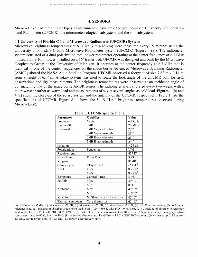
MicroWEX-2 had three major types of instrument subsystems: the ground-based University of Florida C-band Radiometer (UFCMR), the micrometeorological subsystem, and the soil subsystem. 4.1 University of Florida C-band Microwave Radiometer (UFCMR) System Microwave brightness temperatures at 6.7GHz (λ = 4.48 cm) were measured every 15 minutes using the University of Florida’s C-band Microwave Radiometer system (UFCMR) (Figure 4 (a)). The radiometer system consisted of a dual polarization total power radiometer operating at the center frequency of 6.7 GHz housed atop a 10 m tower installed on a 16’ trailer bed. UFCMR was designed and built by the Microwave Geophysics Group at the University of Michigan. It operates at the center frequency at 6.7 GHz that is identical to one of the center frequencies on the space borne Advanced Microwave Scanning Radiometer (AMSR) aboard the NASA Aqua Satellite Program. UFCMR observed a footprint of size 7.62 m X 9.14 m from a height of 6.17 m. A rotary system was used to rotate the look angle of the UFCMR both for field observations and sky measurements. The brightness temperatures were observed at an incidence angle of 55˚ matching that of the space borne AMSR sensor. The radiometer was calibrated every two weeks with a microwave absorber as warm load and measurements of sky at several angles as cold load. Figures 4 (b) and 4 (c) show the close-up of the rotary system and the antenna of the UFCMR, respectively. Table 1 lists the specifications of UFCMR. Figure A-1 shows the V- & H-pol brightness temperatures observed during MicroWEX-2.
Table 1. UFCMR specifications Parameter Qualifier Value Frequency Center 6.7 GHz Bandwidth 3 dB 20 MHz
3 dB V-pol elevation 23°a
3 dB V-pol azimuth 21°b 3 dB H-pol elevation 21°c
Beamwidth
3 dB H-pol azimuth 23°d Isolation > 27 dB Polarizations Sequential V/H Receiver temp 437 Ke Noise Figure From Trec 3.99 dB RF gain 85 dB Gain tempco dTsys/dTset -2 K/Cf
1 sec 0.71 Kg NEDT 8 sec 0.25 Kh
Tempature Control – rms 5 mKi Max 40° Cj SetPoint Min 0° C Max 48° Ck Ambient Min < 0° Cl
RF cutout McShane or RF1 thermistor 42° Cm Thermal shutdown Case thermistor 62° Cn
(a). sidelobes < -33 dB, (b). sidelobes < -28 dB, (c). sidelobes < -27 dB, (d). sidelobes < -35 dB, (e). +/- 20 K uncertainty, (f). looking at reference load, (g). tracking of absorber to reference load in lab, Tset = 305 K with PID = 0.75, 0.94, 0, (h). tracking of absorber to reference load in lab, Tset = 305 K with PID = 0.75, 0.94, 0, (i). Tset = 305 K in lab environment, on RF2, over 0.5 hour, after a day running, (j). active components rated to 65 C, filters to 40 C, (k). estimated absolute max Tamb-Tset = 15 C at TEC 100% cooling, (l). estimated, (m). RF power cut only, user recovery only, (n). RF and TEC power, user recovery only.
Archival copy: for current recommendations see http://edis.ifas.ufl.edu or your local extension office.

5
Figure 4 (a).The UFCMR system
Figure 4 (b) and (c). The side view of the UFCMR showing the rotary system and the front view of the
UFCMR showing the receiver antenna. 4.1.1. Theory of operation UFCMR uses a thermoelectric cooler (TEC) for thermal control of the Radio Frequency (RF) stages for the UFCMR. This is accomplished by the Oven Industries “McShane” thermal controller. McShane is used to cool or heat by Proportional-Integral-Derivative (PID) algorithm with a high degree of precision at 0.01°C. The aluminum plate to which all the RF components are attached is chosen to have sufficient thermal mass to eliminate short-term thermal drifts. All components attached to this thermal plate, including the TEC, use thermal paste to minimize thermal gradients across junctions.
6.17 m
Archival copy: for current recommendations see http://edis.ifas.ufl.edu or your local extension office.
6
The majority of the gain in the system is provided by a gain and filtering block designed by the University of Michigan for the STAR-Light instrument (De Roo, 2003). The main advantage of this gain block is the close proximity of all the amplifiers, simplifying the task of thermal control. This gain block was designed for a radiometer working at the radio astronomy window of 1400 to 1427 MHz, and so the receiver is a heterodyne type with downconversion from the C-band RF to L-band. To minimize the receiver noise figure, a C-band low-noise amplifier (LNA) is used just prior to downconversion. To protect the amplifier from saturation due to out of band interference, a relatively wide bandwidth, but low insertion loss, bandpass filter is used just prior to the amplifier. Between the filter and the antenna are three components: a switch for choosing polarization, a switch for monitoring a reference load, and an isolator to minimize changes in the apparent system gain due to differences in the reflections looking upstream from the LNA. The electrical penetrations use commercially available weatherproof bulkhead connections (Deutsch connectors or equivalent). The heat sinks have been carefully located employing RTV (silicone sealant) to seal the bolt holes. The radome uses 15mil polycarbonate for radiometric signal penetration. It is sealed to the case using a rubber gasket held down to the case by a square retainer. The first SMA connection electomechanical latching, which is driven by the Z-World control board switches between V- and H-polarization sequentially. The SMA second latching which switches between the analog signal from the first switch and the reference load signal from a reference load resistor sends the analog signal to a isolator, where the signals within 6.4 to 7.2 GHz in radiofrequency are isolated. Then the central frequency is picked up by a 6.7 GHz bandpass filter, which also protects the amplifier to saturation. A Low Noise Amplifier (LNA) is used to eliminate the noise figure and adjust gain. A mixer takes the input from the LNA and a local oscillator to output a 1.4 GHz signal to STAR-Lite. After the Power Amplifier and Filtering Block (Star-Lite back-end), the signal is passed through a Square Law Detector and a Post-Detection Amplifier. UFCMR is equipped with a microcontroller that has responsibility for taking measurements, monitoring the thermal environment, and storing data until a download is requested. A laptop computer is used for running the user interface named FluxMon to communicate with the radiometer through Radiometer Control Language (RadiCL). The radiometer is configured to maintain a particular thermal set point, and make periodic measurements of the brightness at both polarizations sequentially and the reference load. The data collected by the radiometer is not calibrated within the instrument, since calibration errors could corrupt an otherwise useful dataset. Figure 5 shows the block diagram of UFCMR.
Archival copy: for current recommendations see http://edis.ifas.ufl.edu or your local extension office.

7
Figure 5. Block diagram of the University of Florida C-band Radiometer (De Roo, 2002).
4.2 Eddy Covariance System A Campbell Scientific eddy covariance system was located at the center of the field as shown in Figure 3. Figure 6 shows a close up of the sensor. The system included a CSAT3 anemometer and KH20 hygrometer. CSAT3 is a three dimensional sonic anemometer, which measures wind speed and the speed of sound on three non-orthogonal axes. Orthogonal wind speed and sonic temperature are computed from these measurements. KH20 measures the water vapor in the atmosphere. Its output voltage is proportional to the water vapor density flux. Latent and sensible heat fluxes were measured every 15 minutes. The height of the eddy covariance system was 2.1 m from the ground and the orientation of the system was 232° toward southwest. Table 2 shows the list of specifications of the CSAT3. Data collected by the eddy covariance system have been processed for coordinate rotation (Kaimal and Finnigan, 1994; Wilczak et al., 2001), WPL (Web et al., 1980), oxygen (van Dijk et al., 2003, 2004), and sonic temperature corrections (Schotanus et al., 1983). Figure A-2 shows the processed latent and sensible heat fluxes observed during MicroWEX-2.
Archival copy: for current recommendations see http://edis.ifas.ufl.edu or your local extension office.

8
Figure 6. Eddy covariance system
Table 2. Specifications of the CSAT3 (Campbell Scientific, 1998)
Description Value Measurement rate 1 to 60 Hz Noise equivalent wind 1 mm/sec in horizontal wind speed and 0.5 mm/sec in vertical wind speed Wind measurement offset < ±4 cm/sec over –30 to 50ºC Output signals Digital SDM or RS-232 and Analog Digital output signal range ±65.535 m/sec in wind speed and 300 to 366 m/sec in speed of sound Digital output signal resolution 0.25 to 2 mm/sec in vertical wind speed and 1 mm/s in speed of sound Analog output signal range ±32.768 to ±65.536 m/sec in wind speed and 300 to 366 m/sec in speed of sound Analog output signal resolution ±8.192 mm/sec in vertical wind speed and 16 mm/sec in speed of sound Measurement path length 10.0 cm vertical and 5.8 cm horizontal Transducer path angle from horizontal 60 degrees Transducer 0.64 cm in diameter Transducer mounting arms 0.84 cm in diameter Support arms 1.59 cm in diameter Dimensions: anemometer head 47.3 cm x 42.4 cm Dimensions: electronics box 26 cm x 16 cm x 9 cm Dimensions: carry case 71.1 cm x 58.4 cm x 33 cm Weight: anemometer head 1.7 kg Weight: electronics box 2.8 kg Weight: shipping 16.8 kg Operating temperature range -30ºC to 50ºC Power requirement: voltage supply 10 to 16 VDC Power requirement: current 200 mA at 60 Hz measurement rate and 100 mA at 20 Hz measurement rate
4.3 Net Radiometer A Kipp and Zonen CNR-1 four-component net radiometer (Figure 7) was located at the center of the field to measure up- and down-welling short- and long-wave infrared radiation. The sensor consists of two pyranometers (CM-3) and two pyrgeometers (CG-3). The sensor was installed at the height of 2.66 m above ground and facing south. Table 3 shows s the list of specifications of the CNR-1 net radiometer. Figure A-3 shows the up- and down-welling solar (shortwave) wave radiation observed during MicroWEX-2 and the up- and down-welling far infrared (longwave) radiation observed during MicroWEX-2.
Archival copy: for current recommendations see http://edis.ifas.ufl.edu or your local extension office.

9
Figure 7. CNR-1 net radiometer
Table 3. Specifications of the CNR-1 net radiometer (Campbell Scientific, 2004a)
Description Value Measurement spectrum: CM-3 305 to 2800 nm Measurement spectrum: CG-3 5000 t o50000 nm Response time 18 sec Sensitivity 10 to 35 μV/(W/m2) Pt-100 sensor temperature measurement DIN class A Accuracy of the Pt-100 measurement ± 2 K Heating Resistor 24 ohms, 6 VA at 12 volt Maximum error due to heating: CM-3 10 W/m2 Operating temperature -40º to 70ºC Daily total radiation accuracy ± 10% Cable length 10 m Weight 4 kg
4.4 Thermal Infrared (TIR) Sensor An Everest Interscience thermal infrared sensor (4000.3ZL – see Table 4 for specifications) was collocated with the net radiometer to observe skin temperature at nadir. The sensor was installed at the height of 2.5 m. With the sensor field of view of 15º, the size of the footprint for the thermal infrared sensor was 66 cm X 66 cm. Figure A-1 shows the surface thermal infrared temperature observed during MicroWEX-2.
Table 4. Specifications of the thermal infrared sensor (Everest Interscience, 2005) Description Value
Accuracy ± 0.5ºC Resolution 0.1ºC Measurement range -40º to 100ºC Measurement spectrum 8 to 14 µm Field of view 15º Response time 0.1 sec Operating distance 2 cm to 300 m Power requirement: voltage supply 5 to 26 VDC Power requirement: current 10 mA Output signal RS-232C and analog mV (10.0 mV/ºC)
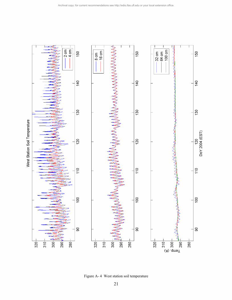
4.5 Soil Moisture and Temperature Probes Five standard Vitel Hydra soil moisture and temperature probes and ten Campbell Scientific time-domain water content reflectometers (CS616 – see Table 5 for calibration coefficients) were used to measure soil volumetric water content and temperature at depths of 2, 4, 8, 16, 32, 64, and 100 cm in row every 15 minutes. The observations of soil moisture were duplicated at the depth of 2 cm in the northwest station. The calibration coefficients for the CS616 probes are listed in Table 2. Figure A-4 shows the soil temperatures observed at the depths of 2cm, 4cm, 8cm, 16cm, 32cm, 64cm, and 100cm at northwest station during MicroWEX-2. The data from the temperature probe at 2cm could not be included because the probe
Archival copy: for current recommendations see http://edis.ifas.ufl.edu or your local extension office.
10
was malfunctioning. Figure A-5 shows the soil temperatures observed at the same depths at east station. Figure A-6 show the volumetric soil moisture content observed at the same depths at northwest station. Figure A-7 shows the volumetric soil moisture content observed at the same depths at east station.
Table 5. The calibration coefficients for the CS616 probes (Campbell Scientific, 2004b) Coefficient Value
C0 -0.187 C1 0.037 C2 0.335
4.6 Soil Heat Flux Plates Two Campbell Scientific (2003) soil heat flux plates (HFT-3) were used to measure soil heat flux at the depths of 2 and 5 cm, in row and near the root area at the Northwest station. Figure A-8 shows the soil heat fluxes observed at 2cm and 5cm at northwest station and the soil heat fluxes observed at 2cm and 3cm at the East station.
5. SOIL SAMPLING
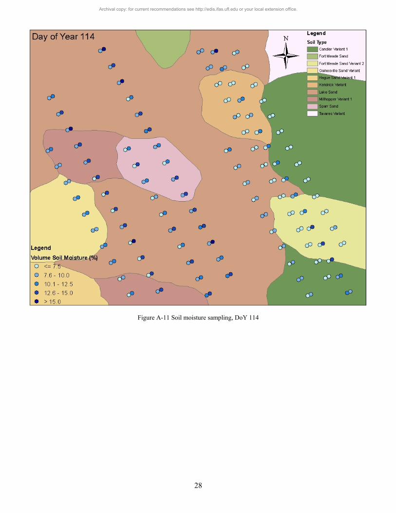
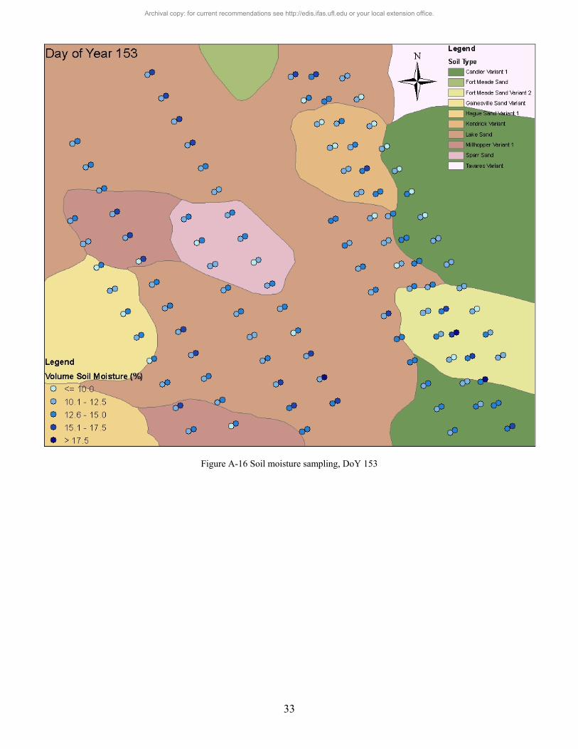
5.1 Soil Moisture An ML2 theta probe volumetric soil moisture sensor from Delta-T Devices was used to measure the soil moisture in the top 6 cm in-row and between-row along 8 transects at the specific locations shown in Figure 8. Spatial soil moisture plots are shown in Figures A-9 through A-16. 5.2 Soil Temperature A Max/Min waterproof digital thermometer from Forestry Supplier was used to measure the soil temperature at the depths of 2, 4, and 8 cm at the same locations and time as the soil moisture sampling. The near surface soil temperature especially at the depth of 2 cm changed rapidly. This was primarily due to the canopy cover, which was not uniform throughout the field. Spatial soil temperature plots for each soil sampling date are shown in Figures A-17 through 24.
Archival copy: for current recommendations see http://edis.ifas.ufl.edu or your local extension office.

11
Figure 8. Layout of the soil sampling locations
Archival copy: for current recommendations see http://edis.ifas.ufl.edu or your local extension office.

12
6. VEGETATION SAMPLING
Vegetation properties such as stand density, row spacing, height, biomass, and LAI were measured weekly during the field experiment. The crop density derived from the stand density and row spacing was measured at the first two samplings since the corn seeds were planted in the fixed spacing and the germination rate was over 70% throughout the field. The specific weekly measurements include height, biomass, and LAI. In the whole season, the vegetation samplings were conducted on four spatially distributed sampling locations (Figure 3). It was designed to characterize the spatial variability of the vegetation properties in the study site. 6.1 Height Crop height was measured by placing a measuring stick at the soil surface up to average height of the crop. The heights inside the vegetation sampling areas were taken for each vegetation sampling. Crop height for each vegetation area is shown in Figure A-25. 6.2 LAI LAI was measured with a Li-Cor LAI-2000 in the inter-row region with 4 cross-row measurements. The LAI-2000 was set to average 2 locations into a single value for each vegetation sampling area so one observation was taken above the canopy and 4 beneath the canopy; in the row, ¼ of the way across the row, ½ of the way across the row, and ¾ of the way across the row. This gave a spatial average for row crops of partial cover. LAI for each vegetation area is shown in Figure A-25. 6.3 Green and Dry Biomass Each biomass sampling included one row. The sampling length was measured the same as length during stand density measurement. The sample started in-between two plants and ended at the next midpoint that is also greater than or equal to one meter away from the starting point. The plants within this length were cut at the base, separated into leaves, stems, and ears, and weighed immediately. The samples were dried in the oven at 70ºC for 48 hours and their dry weights were measured, separating the ears into husks, shucks, and kernel/cobs. Figure A-26 shows the Green and Dry biomass observed during MicroWEX-2, as well as height and LAI. 6.4 Root Length Density At tasseling, root samples were taken with a soil coring tool in the East and West sides of the field, in-between rows and in-between plants, at depths of 0-15, 15-30, 30-60, 60-90, and 90-120 cm. After cleaning the samples, root length density was determined using a scanner and the WinRhizo software. Figure A-27 shows root length density at the midpoints of the specified depths.
7. WELL SAMPLING
7.1 Groundwater sampling The groundwater sampling was conducted by Dr. Michael Dukes and his research team. The sampling was conducted at all four wells in the field at the end of each month from March to June in 2004. The groundwater sampling included groundwater level measurement by water level sounder, and collecting groundwater samples for the analysis of N2. Fertigation rates and soil NO3
- and soil NH4+ are shown in
Figure A-28. 7.2 Water level measurement The water level measurement was processed by the Levelogger from Solinst Canada Ltd.. The Leveloggers were installed at each well and set to record automatically the water level every 15 minutes. Personnel from CRS downloaded the data onto a laptop during the well sampling at the end of each month. Water table depth and elevation are shown in Figure A-29.
Archival copy: for current recommendations see http://edis.ifas.ufl.edu or your local extension office.

13
7.3 Precipitation Precipitation was determined using four tipping-bucket raingages, two on either side of the footprint and two on either side of the field. In addition, Dr. Dukes kept a record of precipitation, fertigation, and irrigation on a daily basis. Figure A-30 shows the precipitation at the raingages and irrigation, fertigation and precipitation from Dr. Duke’s record.
8. FIELD LOG
Note: Time is in Eastern Standard Time.
March 17 (DoY 77)
09:00 Monitoring wells installed 12:15 Marked rows, tested radiometer
March 18 (DoY 78)
09:00 Planting, except in NE and SW corners; Plant population: ~250000; Row spacing: 76.2 cm; Plant Density: 8.03 plants/m2
March 19 (DoY 79)
09:30 Installed tower and radiometer, marked footprint 14:30 Installed Eddy Covariance System
March 22 (DoY 82)
13:10 Found McShane had overheated; radiometer calibration 13:50 Replaced desiccants; run temperature control 17:30 Radiometer is left off as cover was being repaired
March 23 (DoY 83)
14:00 Installed West station 32 cm, 64 cm, 1m soil moisture and temperature sensors
Installed CR23X, CSAT3, KH2O (2.1 m) Planted in NE, SW corners
March 24 (DoY 84)
11:30 Complete sensor installation at East station; finished sensor installation at Northwest station
March 25 (DoY 85)
10:00 Partial germination; datalogger programs loaded March 26 (DoY 86)
14:00 Marked row numbers and tractor rows; majority germinated March 29 (DoY 89)
14:00 Installed the first heat flux plate on the West side 14:20 Changed battery for CSAT
Archival copy: for current recommendations see http://edis.ifas.ufl.edu or your local extension office.

14
March 31 (DoY 91)
08:30 Re-soldered H-V & V-H at the H/V switch 13:00 Checked radiometer data, looked reasonable 14:00 Seeds replanted in footprint 15:00 Soil sampling
April 2 (DoY 93)
08:45 Found problem with radiometer data: H-pol starts to match V-pol on DoY 92; radiometer taken down
10:00 CR23X code changed for CSAT 11:00 Marked vegetation sampling areas and soil sampling transects 12:00 Soil sampling
April 5 (DoY 96)
08:45 Found a bad transistor; replaced it and undid change on H/V switch
14:00 Radiometer in the field April 7 (DoY 98)
09:00 Installed second soil heat flux plate on west side April 8 (DoY 99)
09:00 Crop cultivated 09:20 Cultivated near footprint 10:00 East 4, 16 cm TDR run over by tractor 10:30 Removed 2 cm soil heat flux plate
April 9 (DoY 100)
09:00 Vegetation sampling 10:00 Soil sampling
April 12 (DoY 103)
11:40 Footprint hand cultivated to remove weeds April 16 (DoY 107)
09:00 Vegetation sampling 10:00 Soil sampling
April 20 (DoY 111) April 23 (DoY 114)
10:00 Soil sampling April 27 (DoY 118)
09:15 Radiometer calibrated
09:00 Vegetation sampling
Archival copy: for current recommendations see http://edis.ifas.ufl.edu or your local extension office.

15
April 30 (DoY 121) 09:00 Vegetation sampling 10:00 Soil sampling
May 4 (DoY 125)
09:00 Vegetation sampling May 7 (DoY 128)
09:00 Vegetation sampling 10:00 Soil sampling
May 11 (DoY 132)
09:00 Vegetation sampling May 14 (DoY 135)
09:00 Vegetation sampling 10:00 Soil sampling
May 18 (DoY 139)
09:00 Vegetation sampling May 21 (DoY 142)
12:00 Cleaned KH2O sensor head Re-install footprint raingages Vegetation sampling Soil sampling
June 1 (DoY 153)
12:35 Radiometer calibration Footprint LAI samples Soil sampling
June 2 (DoY 154)
08:35 Theta probe sampling in footprint 10:00 Disconnect sensors Harvest
Archival copy: for current recommendations see http://edis.ifas.ufl.edu or your local extension office.

16
9. REFERENCES
Campbell Scientific, CSAT3 Three Dimensional Sonic Anemometer Instruction Manual, Campbell Scientific Inc., Logan, UT, 1998.
Campbell Scientific, HFT3 soil heat flux plate instruction manual, Campbell Scientific Inc., Logan, UT,
2003. Campbell Scientific, CNR1 Net Radiometer Instruction Manual, Campbell Scientific Inc., Logan, UT,
2004a.
Campbell Scientific, CS615 andCS625 water content reflectometers instruction manual, Campbell Scientific Inc., Logan, UT, 2004b.
Everest Interscience, Model 4000.3ZL Infrared Temperature Sensor, Everest Interscience Inc., Tuson, AZ,
2005. J. C. Kaimal and J. J. Finnigan, Atmospheric Boundary Layer Flows, Oxford University Press, New York,
NY, 1994. R. D. De Roo, University of Florida C-band Radiometer Summary, Space Physics Research Laboratory,
University of Michigan, Ann Arbor, MI, March, 2002. R. D. De Roo, TMRS-3 Radiometer Tuning Procedures, Space Physics Research Laboratory, University of
Michigan, Ann Arbor, MI, March, 2003. P. Schotanus, F. T. M. Nieuwstadt, and H. A. R. DeBruin, “Temperature measurement with a sonic
anemometer and its application to heat and moisture fluctuations,” Bound.-Layer Meteorol., vol. 26, pp. 81-93, 1983.
A. van Dijk, W. Kohsiek, and H. A. R. DeBruin, “Oxygen sensitivity of krypton and Lyman-alpha
hygrometer,” J. Atmos. Ocean. Tech., vol. 20, pp. 143-151., 2003. A. van Dijk, A. F. Moene, and H. A. R. DeBurin, The Principles of Surface Flux Physics: Theory, Practice,
and Description of the ECPACK Library, http://www.met.wau.nl/projects/jep/, 2004. E. K. Webb, G. I. Pearman, and R. Leuning, “ Correction of flux measurements for density effects due to
heat and water vapor transfer,” Quart. J. Roy. Meteorol., Soc., vol. 106, pp. 85-100, 1980. J. M. Wilczak, S. P. Oncley, and S. A. Stage, “Sonic anemometer tilt correction algorithms,” Bound.-Layer
Meteorol., vol. 99, pp. 127-150, 2001.
Archival copy: for current recommendations see http://edis.ifas.ufl.edu or your local extension office.

17
10. ACKNOWLEDGEMENTS
This research was supported by funding obtained from the NSF-Earth Science Directorate, Grant Number EAR-0337277. The authors would like to thank Mr. James Boyer and his team at the PSREU for land and crop management.
A. FIELD OBSERVATIONS Figure Captions Figure A-1 Microwave brightness at vertical and horizontal polarizations; surface temperature…………..18 Figure A-2 Latent and sensible heat fluxes………………………………………………………………….19 Figure A-3 Down- and up- welling short- and long- wave radiation…………………….………………….20 Figure A-4 West station soil temperature..……………………………………………….………………….21 Figure A-5 East station soil temperature.….………………………………………………………………...22 Figure A-6 West station soil moisture……………………………………………………………………….23 Figure A-7 East station soil moisture………………………………………………………….……………..24 Figure A-8 West and East station soil heat fluxes……………………………………………...……………25 Figure A-9 Soil moisture sampling, DoY 100………………………………………………….……………26 Figure A-10 Soil moisture sampling, DoY 107…..……………………………………………….…………27 Figure A-11 Soil moisture sampling, DoY 114…..……………………………………………….…………28 Figure A-12 Soil moisture sampling, DoY 121…..……………………………………………….…………29 Figure A-13 Soil moisture sampling, DoY 128…..……………………………………………….…………30 Figure A-14 Soil moisture sampling, DoY 135…..……………………………………………….…………31 Figure A-15 Soil moisture sampling, DoY 142…..……………………………………………….…………32 Figure A-16 Soil moisture sampling, DoY 153…..……………………………………………….…………33 Figure A-17 Soil temperature sampling, DoY 100………………..…………………………………………34 Figure A-18 Soil temperature sampling, DoY 107…..…………………………………………….………...35 Figure A-19 Soil temperature sampling, DoY 114…..………………………………………………………36 Figure A-20 Soil temperature sampling, DoY 121…..…………………………...……………….…………37 Figure A-21 Soil temperature sampling, DoY 128…..………………………………………………………38 Figure A-22 Soil temperature sampling, DoY 135…..………………………………………………………39 Figure A-23 Soil temperature sampling, DoY 142…..………………………………………………………40 Figure A-24 Soil temperature sampling, DoY 153…..…………………………………………….………...41 Figure A-25 Canopy height and LAI………………………………………………………………..……….42 Figure A-26 Wet and dry canopy biomass…………………………………………………………………..43 Figure A-27 Root length density at tasseling……………………………………………………………..…44 Figure A-28 Fertigation applications and soil nitrogen by depth………………………………...………….45 Figure A-29 Water table depth and elevation…………………………………………………………….….46 Figure A-30 Precipitation ….………………………………………………………………………………..47
Archival copy: for current recommendations see http://edis.ifas.ufl.edu or your local extension office.

18
Figure A- 1 Microwave brightness at vertical and horizontal polarizations; surface temperature
Archival copy: for current recommendations see http://edis.ifas.ufl.edu or your local extension office.

19
Figure A- 2 Latent and sensible heat fluxes
Archival copy: for current recommendations see http://edis.ifas.ufl.edu or your local extension office.

20
Figure A- 3 Down- and up- welling short- and long- wave radiation
Archival copy: for current recommendations see http://edis.ifas.ufl.edu or your local extension office.
21
Figure A- 4 West station soil temperature
Archival copy: for current recommendations see http://edis.ifas.ufl.edu or your local extension office.

22
Figure A- 5 East station soil temperature
Archival copy: for current recommendations see http://edis.ifas.ufl.edu or your local extension office.

23
Figure A- 6 West station soil moisture
Archival copy: for current recommendations see http://edis.ifas.ufl.edu or your local extension office.

24
Figure A- 7 East station soil moisture
Archival copy: for current recommendations see http://edis.ifas.ufl.edu or your local extension office.

25
Figure A- 8 West and East station soil heat fluxes
Archival copy: for current recommendations see http://edis.ifas.ufl.edu or your local extension office.

26
Figure A-9. Soil moisture sampling, DoY 100
In furrow
In row
Archival copy: for current recommendations see http://edis.ifas.ufl.edu or your local extension office.

27
Figure A-10 Soil moisture sampling, DoY 107
Archival copy: for current recommendations see http://edis.ifas.ufl.edu or your local extension office.
28
Figure A-11 Soil moisture sampling, DoY 114
Archival copy: for current recommendations see http://edis.ifas.ufl.edu or your local extension office.

29
Figure A-12 Soil moisture sampling, DoY 121
Archival copy: for current recommendations see http://edis.ifas.ufl.edu or your local extension office.

30
Figure A-13 Soil moisture sampling, DoY 128
Archival copy: for current recommendations see http://edis.ifas.ufl.edu or your local extension office.

31
Figure A-14 Soil moisture sampling, DoY 135
Archival copy: for current recommendations see http://edis.ifas.ufl.edu or your local extension office.

32
Figure A-15 Soil moisture sampling, DoY 142
Archival copy: for current recommendations see http://edis.ifas.ufl.edu or your local extension office.
33
Figure A-16 Soil moisture sampling, DoY 153
Archival copy: for current recommendations see http://edis.ifas.ufl.edu or your local extension office.

34
Figure A-17 Soil temperature sampling, DoY 100
Depth (cm): 2 4 8
Archival copy: for current recommendations see http://edis.ifas.ufl.edu or your local extension office.

35
Figure A-18 Soil temperature sampling, DoY 107
Archival copy: for current recommendations see http://edis.ifas.ufl.edu or your local extension office.

36
Figure A-19 Soil temperature sampling, DoY 114
Archival copy: for current recommendations see http://edis.ifas.ufl.edu or your local extension office.

37
Figure A-20 Soil temperature sampling, DoY 121
Archival copy: for current recommendations see http://edis.ifas.ufl.edu or your local extension office.

38
Figure A-21 Soil temperature sampling, DoY 128
Archival copy: for current recommendations see http://edis.ifas.ufl.edu or your local extension office.
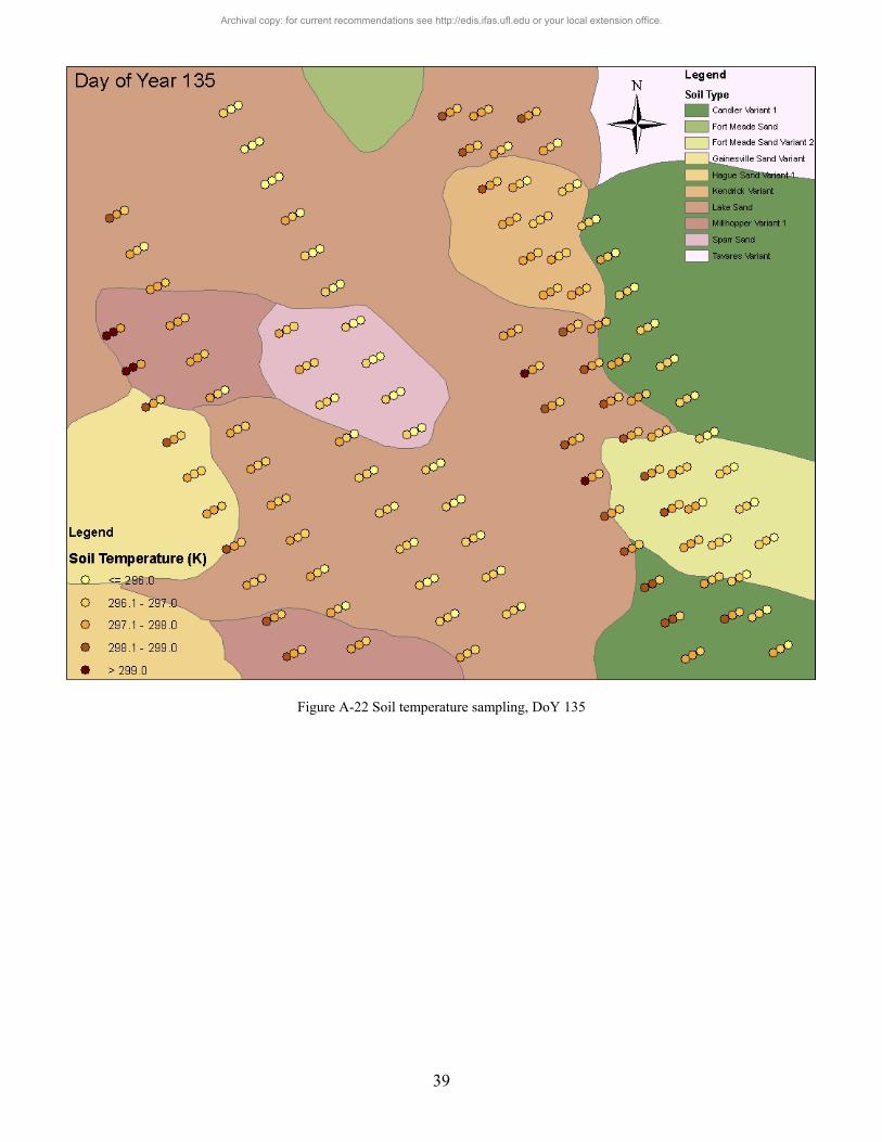
39
Figure A-22 Soil temperature sampling, DoY 135
Archival copy: for current recommendations see http://edis.ifas.ufl.edu or your local extension office.

40
Figure A-23 Soil temperature sampling, DoY 142
Archival copy: for current recommendations see http://edis.ifas.ufl.edu or your local extension office.
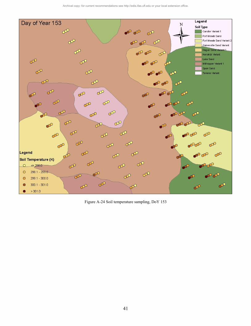
41
Figure A-24 Soil temperature sampling, DoY 153
Archival copy: for current recommendations see http://edis.ifas.ufl.edu or your local extension office.

42
Figure A- 25 Canopy height and LAI
Archival copy: for current recommendations see http://edis.ifas.ufl.edu or your local extension office.

43
Figure A- 26 Wet and dry canopy biomass
Archival copy: for current recommendations see http://edis.ifas.ufl.edu or your local extension office.

44
Figure A- 27 Root length density at tasseling
Archival copy: for current recommendations see http://edis.ifas.ufl.edu or your local extension office.

45
Figure A- 28 Fertigation applications and soil nitrogen by depth
Archival copy: for current recommendations see http://edis.ifas.ufl.edu or your local extension office.

46
Figure A- 29 Water table depth and elevation
Archival copy: for current recommendations see http://edis.ifas.ufl.edu or your local extension office.

47
Figure A- 30 Precipitation
Archival copy: for current recommendations see http://edis.ifas.ufl.edu or your local extension office.